Article

Dynamic Multi-Population Mutation Architecture-Based Equilibrium Optimizer and Its Engineering Application

School of Automation, Beijing Institute of Technology, Beijing 100081, China
*
Author to whom correspondence should be addressed.
Appl. Sci. 2025, 15(4), 1795; https://doi.org/10.3390/app15041795
Submission received: 6 January 2025 / Revised: 4 February 2025 / Accepted: 5 February 2025 / Published: 10 February 2025

Abstract

:
To strengthen the population diversity and search capability of equilibrium optimizer (EO), a dynamic multi-population mutation architecture-based equilibrium optimizer (DMMAEO) is proposed. Firstly, a dynamic multi-population guidance mechanism is constructed to enhance population diversity. Secondly, a dynamic Gaussian mutation-based sub-population concentration updating mechanism is introduced to strengthen exploitation ability. Finally, a dynamic Cauchy mutation-based sub-population equilibrium candidate generation mechanism is integrated to boost exploration ability. The optimization ability of DMMAEO is assessed through a comparison with several recent promising algorithms on 58 test functions (including 29 representative test functions and 29 CEC2017 test functions). The comparison results reveal that the DMMAEO has superiority in the performance assessment of seeking global optimum over other compared algorithms. The DMMAEO is further employed in addressing six engineering design problems and a UGV multi-target path planning problem. The results show the practicality of DMMAEO in addressing engineering application tasks. The aforementioned numerical optimization and engineering application experimental results show that the three enhancement mechanisms of DMMAEO improve the optimization ability of the canonical EO, and the DMMAEO has competitiveness in tackling various kinds of complex numerical optimization and engineering application problems.

1. Introduction

Optimization problems exist extensively in various domains, including industry [1], agriculture [2], and finance [3]. The methods for solving optimization problems have two main families: traditional mathematical methods and intelligent optimization methods [4]. However, with the advancement of science and technology and the growth of task requirements, optimization problems have gradually began to present complex characteristics such as non-differentiability, multimodality, and non-linearity. These complex characteristics limit the capability of traditional mathematical methods in addressing optimization problems. In contrast, intelligent optimization algorithms are effective in handling optimization problems with such complex characteristics. Therefore, more and more researchers are beginning to pay attention to intelligent optimization algorithms and propose a series of new intelligent optimization algorithms, such as grey wolf optimizer (GWO) [5], harris hawks optimizer (HHO) [6], slime mould algorithm (SMA) [7], particle swarm optimizer (PSO) [8], doctor and patient optimizer (DPO) [9], and so on. Although numerous intelligent optimization algorithms have been proposed and used to solve various optimization problems, no optimization algorithm can solve all kinds of optimization problems according to the “No Free Lunch Theorem” (NFL) [10]. And one optimization algorithm may perform better in solving certain optimization problems than others. Therefore, looking for new intelligent optimization algorithms has always been the research focus of relevant researchers in this field.
As a novel intelligent optimization approach based on physical law, equilibrium optimizer (EO) [11] has been recently introduced by Faramarzi et al. EO is implemented by iteratively updating the particle concentrations and generating the equilibrium candidates. Due to its advantages of simple structure, easy realization, fast response speed, and strong optimization capability, EO has been widely used in addressing optimization problems from various fields. In [12], EO was employed in handling the optimal power flow problem by Nusair et al. In [13], EO was applied in the prediction of traffic transportation by combining with a convolutional neural network. In [14], EO was utilized to search for the optimal path with human-like driving styles in a structured road environment. In [15], EO was employed in improving the fusion parameters of low-frequency parts in multimodal medical image processing by Dinh et al. In [16], EO was applied in integrating with the random vector functional link network to predict laser cutting parameters by Elsheikh et al.
Furthermore, to improve EO’s optimization performance for specific requirements, various EO variants have been developed by the researchers. In [17], a local minima elimination approach and a linear reduction diversity strategy are embedded in EO to enhance the convergence. The exploration ability of EO was enhanced by integrating the escape mechanism and the opposition-based learning strategy in [18]. In [19], Too et al. integrated a general learning approach with EO to enhance the ability of searching promising regions. Liu et al. [20] presented an adaptive equilibrium optimizer by integrating EO with the adaptive proportional mutation approach, random walk mechanism, and spiral encirclement method, which strengthens the optimization ability in handling the engineering and complex function optimization problems. By effectively using the information of whole population, neighborhood space, and opposite space, an ameliorated equilibrium optimizer was developed in [21] to enhance the optimization performance of addressing the smooth path planning problem. However, in addressing complex optimization problems, more attention should be paid on how to enhance the population diversity.
Multi-population technology is an effective method to enhance population diversity by partitioning the population into multiple sub-populations and utilizing each sub-population to independently search the optimization space [22]. Based on the above advantage, multi-population technology has been employed to improve diverse optimization algorithms in recent years, such as multi-population PSO [23], multi-population whale optimization algorithm (WOA) [24], multi-population sine cosine algorithm (SCA) [25], multi-population differential evolution (DE) [26], and so on. Multi-population technology assists the above multi-population algorithms to preserve the population diversity during the optimization process. However, multi-population technology has two main categories: dynamic architecture and static architecture. The dynamic architecture raises the cost of the algorithm, while the static architecture is ineffective for the convergence of the algorithm [27]. Therefore, how to design an efficient and simple multi-population architecture is still a challenging research topic.
In EO, the iterative search for optimal solution is implemented based on equilibrium candidate generation and particle concentration updating. If the equilibrium candidates of EO are pooled together within the local optimum area, this search pattern may result in the problems of population diversity decline and premature convergence. This search pattern relies too much on the equilibrium candidates generated by the whole population and lacks the effective utilization of the sub-population structure and information within the population updating process. The above shortcomings of EO limit its search capability in the optimization space. To alleviate the above problems of EO, a dynamic multi-population mutation architecture-based equilibrium optimizer (DMMAEO) is proposed. By constructing a sub-population structure and using sub-population information, the particle concentration updating stage and equilibrium candidate generation stage of the DMMAEO are altered in the following way. At first, the sub-population structure and corresponding information interaction mode are constructed by introducing a dynamic multi-population guidance mechanism for enhancing population diversity. Then, the neighborhood space information of sub-population particle concentrations is used by integrating dynamic Gaussian mutation to strengthen the exploitation ability. Finally, the promising space information of sub-population equilibrium candidates is employed by combining dynamic Cauchy mutation to improve the exploration ability. To summarize, the major contributions from this study are shown below.
(1)
A dynamic multi-population guidance mechanism is constructed for the whole population, which can enhance the population diversity by utilizing the sub-population structure and information.
(2)
A dynamic Gaussian mutation-based sub-population concentration updating mechanism is introduced, which can improve the exploitation ability by using the neighborhood information of sub-population particle concentrations.
(3)
A dynamic Cauchy mutation-based sub-population equilibrium candidate generation mechanism is integrated, which can strengthen the exploration ability by extending the search space for sub-population equilibrium candidates.
(4)
The optimization performance of DMMAEO is analyzed through comparing it with multiple recent promising algorithms across 58 test functions.
(5)
The practicality of DMMAEO is further verified by applying the the DMMAEO to address six engineering design problems and a UGV multi-target path planning problem.
Section 2 gives an overview of EO’s structure. Section 3 offers a detailed explanation of the specifics regarding DMMAEO. Section 4 shows the test experiments and discussion of DMMAEO on 58 test functions. Section 5 presents the performance of DMMAEO in addressing engineering application problems.

2. Structure of Equilibrium Optimizer (EO)

As an innovative physical law-based intelligent optimization algorithm, EO is developed from the inspiration of dynamic mass balance phenomenon within the control volume [11]. Particle concentration updating and the equilibrium candidate generation are the two primary components of EO. When EO is applied to handle optimization problems, these two primary components are iteratively implemented to seek the global optimum. The particle concentrations signify the position of solutions, and the equilibrium candidates denote the position of best solutions achieved until now. Under the guidance of the generated equilibrium candidates, the particle concentrations are updated to discover superior solutions according to the specific way characterized in the mass balance equation. A concise description about the fundamental phases and mechanisms involved in EO is presented by the subsequent subsections.

2.1. Concentration Initialization

The particle concentration updating and the equilibrium candidate generation in EO are performed based on a dynamic evolution process driven by the population, which implies that initial population formation is required for the subsequent execution of optimization mechanisms. Hence, EO employs a uniform random distribution to formulate its initial population during the initialization phase, which is expressed as
P i ( g = 1 ) = P lb + r 1 P ub P lb , i = 1 , 2 , 3 , , N ,
where N denotes the total amount for particles within the population, r 1 is a random vector ranging in the interval [ 0 , 1 ] , P ub and P lb stand for the upper ranges and lower ranges in search space, and P i ( g = 1 ) signifies the concentration of i-th particle for initial iteration g = 1 . With the formulated initial population, particle concentration updating and the equilibrium candidate generation of EO are iteratively implemented for seeking equilibrium state in optimization space.

2.2. Equilibrium Candidate Generation

The main target of EO is to seek the equilibrium state in optimization space, which is the global optimum of the optimization problem. However, no prior information about the equilibrium state is available. Therefore, the mechanism of equilibrium candidate generation is established to lead the population of EO in approximating the equilibrium state within the search space, which is expressed as
P pool ( g ) = P α ( g ) ,   P β ( g ) ,   P γ ( g ) ,   P δ ( g ) ,   P avg ( g ) ,
P eq ( g ) = E randi ( P pool ( g ) ) ,
where P pool ( g ) is the equilibrium pool constructed by five equilibrium candidates P α ( g ) ,   P β ( g ) ,   P γ ( g ) ,   P δ ( g ) ,   a n d P avg ( g ) ; P α ( g ) ,   P β ( g ) ,   P γ ( g ) ,   a n d P δ ( g ) , respectively, denote the four best solutions acquired by sorting the fitness values of population particles up to the current iteration; P avg ( g ) represents mean position of the four best solutions; P eq ( g ) is a currently selected equilibrium candidate, which is employed to guide the subsequent process of particle concentration updating; and E randi ( · ) is the random selection function, which is used to randomly select an equilibrium candidate at the same probability in an equilibrium pool.

2.3. Concentration Updating

Concentration updating serves as the core mechanism of EO to effectively search optimization space. Under the guidance of the equilibrium candidates, the particle concentration in EO is updated based on the mass balance equation, which is expressed as
P i ( g + 1 ) = P eq ( g ) + P i ( g ) P eq ( g ) H i ( g ) + ( 1 H i ( g ) ) F i ( g ) ζ i ( g ) V ,
where g indicates the current iteration number; V signifies a unit, which is designated as 1; ζ i ( g ) signifies a turnover rate and is generated by a random vector within the scope of 0 to 1; and P i ( g ) and P i ( g + 1 ) , respectively, denote the i-th particle concentration before and after updating in the g-th iteration.
H i ( g ) is an important term that aids in balancing the exploration performance and exploitation performance of EO, and it is calculated by
H i ( g ) = η 1 sign ( r 2 0.5 ) e ζ i ( g ) t ( g ) 1 ,
t ( g ) = ( 1 g g max ) ( η 2 g g max ) ,
where η 1 and η 2 are two constants utilized to, respectively, modulate exploration performance and exploitation performance, and they are designated as 2 and 1. g max represents the maximum iteration number for the whole optimization process and r 2 signifies a random vector within the scope of 0 to 1; by referring to r 2 , sign ( r 2 0.5 ) regulates the direction of exploratory and exploitative operation.
F i ( g ) denotes the formation rate, which aids in boosting the exploitation capability, and it is calculated by
F i ( g ) = F i , 0 ( g ) H i ( g ) ,
F i , 0 ( g ) = FC i ( g ) P e q ( g ) ζ i ( g ) P i ( g ) ,
FC i ( g ) = 0.5 r 3 , r 4 F P 0 , r 4 < F P ,
where F P is fixed to 0.5, which denotes the formation probability; r 3 and r 4 indicate two random numbers ranging within the interval [ 0 , 1 ] ; and FC i ( g ) represents the formation rate control parameter, which is adjusted by F P .

3. Dynamic Multi-Population Mutation Architecture-Based Equilibrium Optimizer (DMMAEO)

The above structure of EO makes EO have the merits of a simple structure, easy realization, fast response speed, and strong optimization ability. However, EO still suffers from population diversity decline and premature convergence. To deal with these problems mentioned above, a dynamic multi-population mutation architecture-based equilibrium optimizer (DMMAEO) is proposed. By constructing sub-population structure and using sub-population information, the proposed DMMAEO introduces three improvement mechanisms to improve its optimization performance. Firstly, a dynamic multi-population guidance mechanism is established to increase population diversity. Then, a dynamic Gaussian mutation-based sub-population concentration updating mechanism is integrated for strengthening exploitation ability. Finally, a dynamic Cauchy mutation-based sub-population equilibrium candidate generation mechanism is introduced for enhancing exploration performance. The elaborate descriptions for these three improvement mechanisms of DMMAEO are as follows.

3.1. Dynamic Multi-Population Guidance Mechanism

Under the guidance of equilibrium candidates, particles in the canonical EO are regarded as a complete population for seeking the global optimum of the optimization problem. If the equilibrium candidates of EO are gathered together within the local optimum area, the whole population will dynamically evolve towards this region. This situation makes the whole population of EO unable to search the optimization space effectively. Hence, to design a novel population guidance mechanism for EO is pivotal, which contributes to enhancing population’s search efficiency and population diversity in the optimization domain. For the achievement of this purpose, a dynamic multi-population guidance mechanism is introduced to overcome the limitations of EO’s original guidance mechanism.
The effectiveness of multi-population technology in searching the optimization space is mainly realized through processes including population division and information exchange among sub-populations. The traditional population division of multi-population technology is implemented based on a random sequence. Nonetheless, random sequence exhibits a remarkably prolonged period and poor correlation, which leads to the quality degradation of population division and the difficulty in realizing superior optimization performance. Drawing inspiration from [28], the dynamic multi-population guidance mechanism adopts a chaotic sequence for the process of population division. In this way, the whole population are divided through producing a set of strongly correlated chaotic sequences, which can enhance the population division quality and population optimization ability. The population division using a Logistic chaotic sequence is shown as
CS ( i + 1 ) = λ CS ( i ) ( 1 CS ( i ) ) , i = 1 , 2 , 3 , , N 1 ,
[ , I d ] = sort ( CS ) ,
where CS is a chaotic sequence generated by the Logistic map, whose number of elements is identical with the population size N; the initial value CS ( 1 ) is randomly selected between 0 and 1, and its value needs to be different from 0.25, 0.5, and 0.75; λ indicates a control parameter, which is set to 4 to make the Logistic map appear a state of complete chaos; sort ( · ) is a sort function, which is used to convert the chaotic sequence to a positional sequence; and I d represents the positional sequence. With Equations (10) and (11), the specific process of population division with M sub-populations in the dynamic multi-population guidance mechanism is implemented in the following way. Firstly, a chaotic sequence CS is generated by Equation (10), whose length is consistent with the population size N. Then, a positional sequence I d is obtained by Equation (11). Finally, according to the number of positional sequence I d , the population particles are equally divided into M sub-populations to generate the multiple sub-population structure. With this generated structure, sub-population particles are updated under the guidance of the optimal equilibrium candidate in the sub-population instead of the equilibrium candidates in the whole population, which is shown as
P i ( g + 1 ) = P leq ( i ) ( g ) + P i ( g ) P leq ( i ) ( g ) H i ( g ) + ( 1 H i ( g ) ) F i ( g ) ζ i ( g ) V ,
where P leq ( i ) ( g ) represents the sub-population equilibrium candidate, which is the optimal equilibrium candidate in the local sub-population structure of i-th particle at iteration l.
During the process of sub-population updating, reorganization period R p is applied to guide information communication across sub-populations. The value of R p is crucial in the result of this information communication mode. When R p is excessively small, sub-populations will face the problem of an insufficient search; conversely, an overly large R p will induce delayed information exchange among sub-populations. During the early optimization phase, sub-populations should be allocated sufficient time for the search process; during the later optimization phase, sub-populations should engage in timely information exchange to maximize population diversity, which can strengthen the search capability throughout the entire optimization process. Thus, the reorganization period R p within the dynamic multi-population guidance mechanism is calculated in a dynamic form, which is shown as
R p = ceil ( u s ( u s u e ) g ξ g max ) ,
where ceil ( · ) is a rounding function, which is used to round a number in the direction of positive infinity; u e = 10 and u s = 40 denote the lower ranges and upper ranges for R p , respectively; and the coefficient ξ is employed to regulate the role proportion of the dynamic multi-population guidance mechanism throughout the entire optimization process, which is fixed to 0.9. In particular, R p is initialized as 0 to start the entire algorithm, and then it is calculated according to Equation (13) during the process of population evolution.

3.2. Dynamic Gaussian Mutation-Based Sub-Population Concentration Updating Mechanism

The dynamic multi-population guidance mechanism of the previous subsection changes the entire population to a multiple sub-population structure to seek the global optimum. With the aim of further enhancing the exploitation ability, dynamic Gaussian mutation is introduced into the process of sub-population concentration updating.
The Gaussian density function is expressed as
f Gaussian ( z ) = 1 2 π σ 1 2 e ( z μ 1 ) 2 2 σ 1 2 ,
where μ 1 and σ 1 are the average value and standard deviation for each population particle concentration, respectively. By fixing μ 1 and σ 1 to 0 and 1, respectively, this formula is simplified to generate random numbers. Based on the random numbers generated according to the Gaussian distribution, a dynamic Gaussian mutation-based sub-population concentration updating mechanism is established through
GP i ( g ) = P i ( g ) ( 1 + ξ 1 , i G ( z ) ) ,
ξ 1 , i = r a n k i N ( 1 0.9 g g max ) ,
where GP i ( g ) denotes the new concentration of i-th particle constructed by the dynamic Gaussian mutation; G ( z ) is a step vector, which consists of the random numbers generated by the Gaussian density function; ξ 1 , i represents a dynamic Gaussian mutation control coefficient; and r a n k i indicates the fitness value ranking of i-th particle.
In the process of dynamic Gaussian mutation, the random numbers sampled in Gaussian distribution are combined with the dynamic control coefficient to regulate the primitive particle concentrations. The Gaussian distribution has the property of narrow tail, which can make the new particle concentration produced by the Gaussian mutation tend to gather near the primitive particle concentration. This property can enhance the exploitation capability by utilizing the neighborhood information of particle concentrations. Meanwhile, dynamic Gaussian mutation control coefficient plays a role in adjusting the disturbance level of Gaussian mutation. In the evolution process of the whole population, the disturbance level of Gaussian mutation decreases linearly with the change in dynamic control coefficient to conform to the convergence process of the whole population. Moreover, the dynamic control coefficient makes the better particle with higher fitness value ranking have a smaller disturbance level than the worse particle with lower fitness value ranking in the same iteration, so that the whole population can exploit the better particle area more accurately.

3.3. Dynamic Cauchy Mutation-Based Sub-Population Equilibrium Candidate Generation Mechanism

Within the dynamic multi-population guidance mechanism, the process of sub-population concentration updating is guided by sub-population equilibrium candidate. The sub-population equilibrium candidate is generated by selecting the optimal particle in the sub-population. To further enhance the exploration capability, dynamic Cauchy mutation is integrated into the process of sub-population equilibrium candidate generation.
The Cauchy density function is attained by
f Cauchy ( z ) = 1 π σ 2 ( z μ 2 ) 2 + σ 2 2 ,
where μ 2 and σ 2 represent the location and scale parameters of Cauchy distribution, respectively. By setting μ 2 = 0 and σ 2 = 1 , this formula is simplified to generate random numbers in a way similar to the Gaussian mutation. On the basis of the random numbers generated by the Cauchy mutation, a dynamic Cauchy mutation-based sub-population equilibrium candidate generation mechanism is constructed by
CP leq ( i ) ( g ) = P leq ( i ) ( g ) ( 1 + ξ 2 , i C ( z ) ) ,
ξ 2 , i = 1 0.9 g g max ,
where CP leq ( i ) ( g ) indicates the new sub-population equilibrium candidate created by dynamic Cauchy mutation; C ( z ) denotes a step vector, which is composed of the random numbers generated through the Cauchy density function; and ξ 2 , i represents a dynamic Cauchy mutation control coefficient.
By employing the random numbers generated based on the Cauchy distribution and the dynamic Cauchy mutation control coefficient, the dynamic Cauchy mutation regulates the original equilibrium candidate to produce a new equilibrium candidate. In comparison to the Gaussian distribution used in the previous subsection, the Cauchy distribution exhibits the property of having a long flat tail, which can make the Cauchy mutation have a high probability of generating the new equilibrium candidate far from the original equilibrium candidate. This property can be used to strengthen the exploration ability through expanding the search space for the sub-population equilibrium candidates. Meanwhile, the dynamic Cauchy mutation control coefficient regulates the disturbance level of Cauchy mutation on the equilibrium candidate in a linearly decreasing manner. In this way, the exploration ability of the algorithm is greatly enhanced in the early stage, and the exploration ability of the algorithm is retained to some extent in the later stage.
In a nutshell, the DMMAEO is developed for enhancing the optimization capability by introducing three enhancement mechanisms mentioned above. The utilization of dynamic multi-population guidance mechanism contributes to the increase in population diversity. The incorporation of dynamic Gaussian mutation during the sub-population concentration updating stage boosts the local search capability. Within the sub-population equilibrium candidate generation stage, the integration of dynamic Cauchy mutation serves to reinforce the global search ability. Based on the above introduction, Figure 1 presents the flowchart of DMMAEO, and the subsequent content outlines the steps of DMMAEO.
Step 1 Set the related parameters, including current iteration number g, maximum iteration number g max , population size N, particle dimension D, sub-population number M, and reorganization period R p .
Step 2 Randomly initialize the particle concentrations using Equation (1).
Step 3 Judge whether the iteration interval reaches the reorganization period R p . If so, dynamically create the multi-population structure using Equations (10), (11), and (13); otherwise, continue the process of sub-population concentration updating.
Step 4 Decide the sub-population equilibrium candidates P leq ( i ) ( g ) . For the first iteration, the current sub-population equilibrium candidates are decided in accordance with the fitness values from each sub-population particle. After the first iteration, the current sub-population equilibrium candidates are decided according to the fitness values from each sub-population particle and the sub-population equilibrium candidates generated in the previous iteration.
Step 5 Update the sub-population particle concentrations with the guidance of corresponding sub-population equilibrium candidates using Equation (12).
Step 6 Perform the dynamic Gaussian mutation on the sub-population particle concentrations using Equation (15) and choose the superior particles based on the fitness values to construct the new sub-population.
Step 7 Perform the dynamic Cauchy mutation on the sub-population equilibrium candidates using Equation (18) and choose the better candidates as the new sub-population equilibrium candidates based on the fitness values.
Step 8 Repeat Step 3 to Step 7 till g reaches 0.9 g max or the anticipated fitness value is satisfied.
Step 9 Implement the canonical EO using Equations (2)–(4).
Step 10 Repeat Step 9 until g reaches g max or the anticipated fitness value is satisfied.
Step 11 Return the optimal equilibrium candidate of the whole population P α ( g ) .

3.4. Computational Complexity of DMMAEO

For evaluating the runtime of algorithm, the computational complexity is employed as a vital metric in this paper. It encompasses two primary categories: a non-polynomial order and polynomial order. Comparatively, the non-polynomial order is regarded as inefficient, whereas polynomial order is regarded as efficient. This is due to the fact that the complexity of the non-polynomial order algorithm increases dramatically with the increase in the scale of the optimization problem. As a common method used by many researchers [29,30,31], big-O notation is adopted to assess the computational complexity.
The components of population initialization, equilibrium pool generation, particle concentration updating, and particle concentration evaluation determine the total computational complexity of EO. The population initialization needs the complexity O ( N D ) ; the fast sorting approach is adopted by the equilibrium pool generation process, whose worst-case complexity is O ( g max N 2 ) ; the complexity involved in particle concentration updating process is O ( g max N D ) ; and the complexity involved in particle concentration evaluation is O ( g max N ) . Hence, EO has the complexity O ( g max ( N 2 + N D ) ) . The DMMAEO additionally includes a dynamic multi-population guidance mechanism, a dynamic Gaussian mutation-based sub-population concentration updating mechanism, and a dynamic Cauchy mutation-based sub-population equilibrium candidate generation mechanism. The fast sorting method is also adopted by the dynamic multi-population guidance mechanism, which results in the worst-case complexity O ( g max N 2 ) ; the dynamic Gaussian mutation-based sub-population concentration updating mechanism requires complexity O ( g max N D ) ; and the dynamic Cauchy mutation-based sub-population equilibrium candidate generation mechanism requires complexity O ( g max N D ) . According to the above results, the total computational complexity for DMMAEO is O ( g max ( N 2 + N D ) ) .
To summarize, the proposed DMMAEO and the canonical EO have the same computational complexity. This result indicates that the proposed DMMAEO does not introduce additional complexity to the canonical EO and is an efficient algorithm with polynomial order complexity.

4. Test Experiments and Discussion of DMMAEO

The proposed DMMAEO is a strengthened variant of EO on the basis of the dynamic multi-population mutation architecture, which consists of the dynamic multi-population guidance mechanism and dynamic mutation mechanism. To examine the optimization ability of DMMAEO, test experiments are implemented on 58 test functions. The subsequent subsections present the test results and discussion of DMMAEO.

4.1. Test Functions, Experimental Settings, and Performance Indicators

The 58 test functions (TF1–TF58) primarily consist of two groups. The first group comprises 29 representative test functions (TF1–TF29), which can be classified as four types: unimodal (TF1–TF7), multimodal (TF8–TF13), fixed-dimension multimodal functions (TF14–TF23), and composite test functions (TF24–TF29). These 29 representative test functions are widely adopted by researchers [32,33,34]. Among the 29 representative test functions with four distinct categories, unimodal functions, characterized by a single global optimum, are adopted to evaluate the exploitation performance; multimodal functions, featuring multitudinous local optima, are employed in examining the exploration performance; fixed-dimension multimodal functions, possessing multitudinous local optima and fixed dimensions, serve as a benchmark for evaluating the algorithm’s exploration capability within fixed-dimension search space; and composite functions, designed to mimic complex real-world optimization space with numerous local optima and diverse shapes in different areas, are utilized to test the balancing capability between exploration and exploitation. The second group comprises 29 CEC2017 test functions (TF30–TF58). The 29 CEC2017 test functions in the second group are more challenging to further evaluate the optimization performance of the algorithms than the 29 representative test functions in the first group. Therefore, a comprehensive analysis for the optimization performance of algorithms from various aspects can be achieved based on the 58 test functions. The detailed description for these 58 test functions can be obtained from [35].
Through the utilization of 58 test functions, two experimental designs are formulated in the test experiments to investigate the optimization capability of DMMAEO. The first experimental design investigates the impact of the three improvement mechanisms (dynamic multi-population guidance mechanism, dynamic Gaussian mutation-based sub-population concentration updating mechanism, and dynamic Cauchy mutation-based sub-population equilibrium candidate generation mechanism) on the canonical EO. The second experimental design involves analyzing the superiority of DMMAEO through comparing it to multiple recent promising algorithms, including GWO [5], HHO [6], EO [11], SMA [7], PSO [8], MPSO [36], MELGWO [37], LWMEO [20], and EBOwithCMAR [38]. In order to guarantee a fair comparison in the test experiments, identical experimental settings are applied to all the compared algorithms. The population size and particle dimension for each test function are taken as 30. The maximum iteration number for the test experiments is taken as 500. For achieving statistically meaningful results, each compared algorithm is independently implemented on each test function 30 times. All the test experiments are conducted by Matlab R2021b at the computer executing the 64-bit Microsoft Windows 10 operation system with Intel (R) Core (TM) i7-9750H 2.60 GHz CPU and 16 GB RAM.
Based on the experimental settings and test functions mentioned above, the algorithm optimization ability is analyzed using four performance indicators: Ave., Std., Wilcoxon signed rank test, and Friedman test, which provide quantitative performance assessment from different aspects. Ave. represents the average fitness value derived from independent experiments conducted 30 times, which offers insight into the accuracy of the algorithm’s optimization capability. Std. denotes the corresponding standard deviation derived from independent experiments conducted 30 times, which provides an assessment of the algorithm’s stability. Wilcoxon signed rank test [39] is utilized in determining if the DMMAEO exhibits a significant superiority over other algorithms during the comparative experiments. In this paper, the significance level for the Wilcoxon signed-order test is adopted as 0.05, and its corresponding results are expressed as ‛1/0/−1’ to signify whether the DMMAEO has better, similar, or worse performance compared to other algorithms. The application of the Friedman test [40] allows for a statistical analysis of the overall optimization performance. The results of Friedman test is given by the Friedman mean rank, which serves as an indication of overall optimization performance rank for the compared algorithms.

4.2. Impacts of Enhancement Mechanisms on EO

This subsection investigates the impacts of three enhancement mechanisms introduced in the DMMAEO, including the dynamic multi-population guidance mechanism, dynamic Gaussian mutation-based sub-population concentration updating mechanism, and dynamic Cauchy mutation-based sub-population equilibrium candidate generation mechanism. For this purpose, a performance evaluation of the canonical EO and four EO variants (DMEO, GMEO, CMEO, and DMMAEO) is conducted on the 29 representative test functions. Among the four EO variants, DMEO means that EO is only in combination with dynamic multi-population guidance mechanism; GMEO means that EO is only in combination with the dynamic Gaussian mutation-based sub-population concentration updating mechanism; CMEO means that EO is only in combination with the dynamic Cauchy mutation-based sub-population equilibrium candidate generation mechanism; and DMMAEO indicates that EO is in combination with the three enhancement mechanisms simultaneously.
Table 1, Table 2, Table 3, Table 4 and Table 5 list the comparison results of the Ave., Std., Wilcoxon signed rank test, and Friedman test from the canonical EO and four EO variants mentioned above. These comparison results are obtained by implementing each algorithm 30 times independently across each test function. The best results achieved by the various EOs on the 29 representative test functions, as well as the top-performing algorithm within the different EO variants, are presented in bold for highlighting the comparative results.
According to the results in Table 1, Table 2, Table 3 and Table 4, all four EO variants exhibit superior performance compared to EO across most test functions, which reveals that each of the three enhancement mechanisms contributes to improving the optimization ability of the canonical EO. Among the four EO variants, the DMMAEO achieves the best results across 27 of the 29 representative test functions and shows better optimization capability than other variants of EO in most cases, which means that the DMMAEO can obtain the best optimization ability by combining the three enhancement mechanisms simultaneously. Additionally, Figure 2 exhibits the convergence curves for the canonical EO and four EO variants across nine test functions, which is utilized to provide a visual analysis of convergence performance. As per the results given by Figure 2, the DMMAEO exhibits superior convergence speed and convergence accuracy compared to the other four EO variants.
Meanwhile, Table 5 shows the results of the Friedman test and Wilcoxon signed rank test across 29 representative test functions. The Wilcoxon signed rank test results, symbolized by ‛1/0/−1’ in Table 5, indicate that the DMMAEO outperforms EO, DMEO, GMEO, and CMEO on 21, 19, 20, and 21 functions, respectively. These results mean that the DMMAEO significantly performs better than the canonical EO and other EO variants in most test functions. For the overall performance, the Friedman test results given by Table 5 show that the DMMAEO ranks first, followed by DMEO, CMEO, GMEO, and EO. These results mean that the proposed DMMAEO exhibits the most outstanding overall performance among the various EOs.
To summarize, from the above experimental results obtained by the various EOs, all three enhancement mechanisms are helpful to improve the performance for the canonical EO, and the proposed DMMAEO performs best by incorporating all three enhancement mechanisms.

4.3. Scalability Comparison Analysis

The scalability test is conducted in this subsection, which is used to test the optimization performance of the proposed DMMAEO in different dimensions. The scalability experiments are carried out on the optimization problems with 30, 50, and 100 dimensions, respectively. Except for the change in dimension setting, other experimental parameters are consistent with the previous subsection. The results for the scalability tests in different dimensions are shown in Table 6.
According to the results in Table 6, the optimization performance of EO gradually declines with the increase in dimension. In contrast, the optimization ability of DMMAEO remains stable in more functions, although the optimization ability of DMMAEO also declines with the increasing dimensionality. Moreover, the DMMAEO still shows better optimization ability than EO in most functions with the increase in dimension. Therefore, the scalability experiment shows that the proposed DMMAEO has more stable optimization ability than the canonical EO in the case of dimensional change.

4.4. Diversity Comparison Analysis

Diversity is used as a measurement for the distribution of population particles, which plays an important role in forming diverse population during the search process. According to [41], population diversity is measured through D i v , which is calculated by
P ¯ j = 1 N i = 1 N P i , j , i = 1 , 2 , 3 , , N , j = 1 , 2 , 3 , , D ,
D i v j = 1 N i = 1 N P i , j P ¯ j ,
D i v = 1 D j = 1 D D i v j
where P i , j indicates the concentration of i-th particle in j-th dimension; P ¯ j denotes the pivot of particle concentrations in j-th dimension; and D i v represents the diversity of the whole population.
The diversity curves across the nine test functions are shown in Figure 3, whose results are also obtained based on 30 independent experiments across each test function. According to the results of the diversity curves in Figure 3, it can be observed that the proposed DMMAEO exhibits higher diversity than the canonical EO during the search process of different types of test functions, which contributes to improving the ability of the algorithm to jump out of local optimal solutions. The above results mean that the proposed DMMAEO can effectively strengthen the population diversity and search capability.

4.5. Comparative Analysis Between DMMAEO and Other Algorithms

The previous subsection validates the effectiveness of the three enhancement mechanisms, and the proposed DMMAEO emerges as the top performer within diverse EO variants. For further analyzing the superiority of DMMAEO, this subsection conducts a comparative study between the DMMAEO and several recent promising algorithms (EO [11], PSO [8], GWO [5], HHO [6], SMA [7], MPSO [36], MELGWO [37], LWMEO [20], and EBOwithCMAR [38]) on the 58 test functions. These compared algorithms consists of three different categories: the recently established algorithm (EO, PSO, GWO, HHO, and SMA), the improved algorithm (MPSO, MELGWO, and LWMEO), and the top algorithm (EBOwithCMAR). The detailed parameters for the above compared algorithms are set according to the corresponding original literature.
The comparison results of Ave., Std., Wilcoxon signed rank test, and Friedman test are listed in Table 7, Table 8, Table 9, Table 10, Table 11 and Table 12. Similar to the previous subsection, these results are also obtained by conducting each algorithm with 30 independent experiments across each test function. And the top-performing method and best results obtained from the comparative study within these tables are highlighted in bold as well.
Table 7, Table 8, Table 9, Table 10 and Table 11 present the results of Ave. and Std. for the compared algorithms across 58 test functions (TF1–TF58). According to the results in Table 7, Table 8, Table 9, Table 10 and Table 11, the DMMAEO captures the best results on TF1–TF4, TF7, TF9–TF12, TF14, TF16, TF17, TF19–TF21, TF23–TF25, TF28, TF44, TF49, TF50, and TF52–TF57. Regarding other test functions, the DMMAEO also shows competitive optimization capability. Hence, the DMMAEO shows better performance on most test functions compared to other algorithms. This means that the DMMAEO performs better in the comprehensive optimization ability, and especially has advantages in the balancing ability between exploration and exploitation. In addition, Figure 4 presents convergence curves for the algorithms involved in the comparative study on nine test functions. According to the illustrated results given by Figure 4, the DMMAEO exhibits superior convergence speed and accuracy than other compared algorithms.
In the meantime, the results of the Friedman test and Wilcoxon signed rank test obtained from across 58 test functions are given in Table 12, which are employed to assess the statistical significance for the superiority of DMMAEO. As per the Wilcoxon signed rank test results expressed as ‛1/0/−1’, Table 12 shows that the DMMAEO exhibits superior optimization capability over EO, PSO, GWO, HHO, SMA, MPSO, MELGWO, LWMEO, and EBOwithCMAR across 46, 49, 56, 52, 49, 47, 54, 48, and 28 functions, respectively. This result denotes that the DMMAEO has significant superiority on most test functions compared to other algorithms. According to the Friedman test results given by Table 12, the DMMAEO holds the top rank. It is worth noting that the top algorithm EBOwithCMAR achieves high optimization performance through a complex mechanism, while DMMAEO still exhibits competitive optimization performance compared to EBOwithCMAR. Thus, the DMMAEO performs the strongest overall optimization capability within the algorithms involved in the comparative study from a statistical perspective.
To summarize, in accordance with the aforementioned experimental results acquired by the compared algorithms, the DMMAEO exhibits better optimization performance in terms of convergence ability, exploitation ability, exploration ability, and balance ability between exploitation and exploration.

4.6. Running Time Comparison Analysis

The running time is investigated in this subsection, whose results are also obtained based on 30 independent experiments across each test functions. The results of the average running time across the 58 test functions are shown in Table 13. According to the results in Table 13, the running time of DMMAEO is less than EBOwithCMAR, and is slightly more than the other compared algorithms. Considering the superior optimization performance of DMMAEO obtained in the previous subsections, the running time of DMMAEO is within an acceptable level. Moreover, it is worth noting that DMMAEO achieves competitive optimization performance with less running time compared to the top algorithm EBOwithCMAR.
Therefore, according to the results from Section 4.5 and Section 4.6, Table 14 provides a comprehensive overview of the performance comparison between the proposed DMMAEO and other algorithms. From the results in Table 14, it can be seen that the proposed DMMAEO has advantages in terms of the average fitness value. Meanwhile, the DMMAEO shows disadvantages in terms of the average running time compared to most other algorithms. However, the average running time of DMMAEO is lower than the top algorithm EBOwithCMAR. Based on the above comprehensive overview of the performance comparison results, the DMMAEO is a competitive and acceptable high performance optimizer.

5. DMMAEO for Engineering Application Problems

The above section validates the effectiveness and superiority for the DMMAEO on the 58 test functions. To further analyze the practicability for the DMMAEO, two types of engineering application problems are addressed using the DMMAEO. The first type of engineering application problem comprises six engineering optimization problems, including three-bar truss design (EA1) [
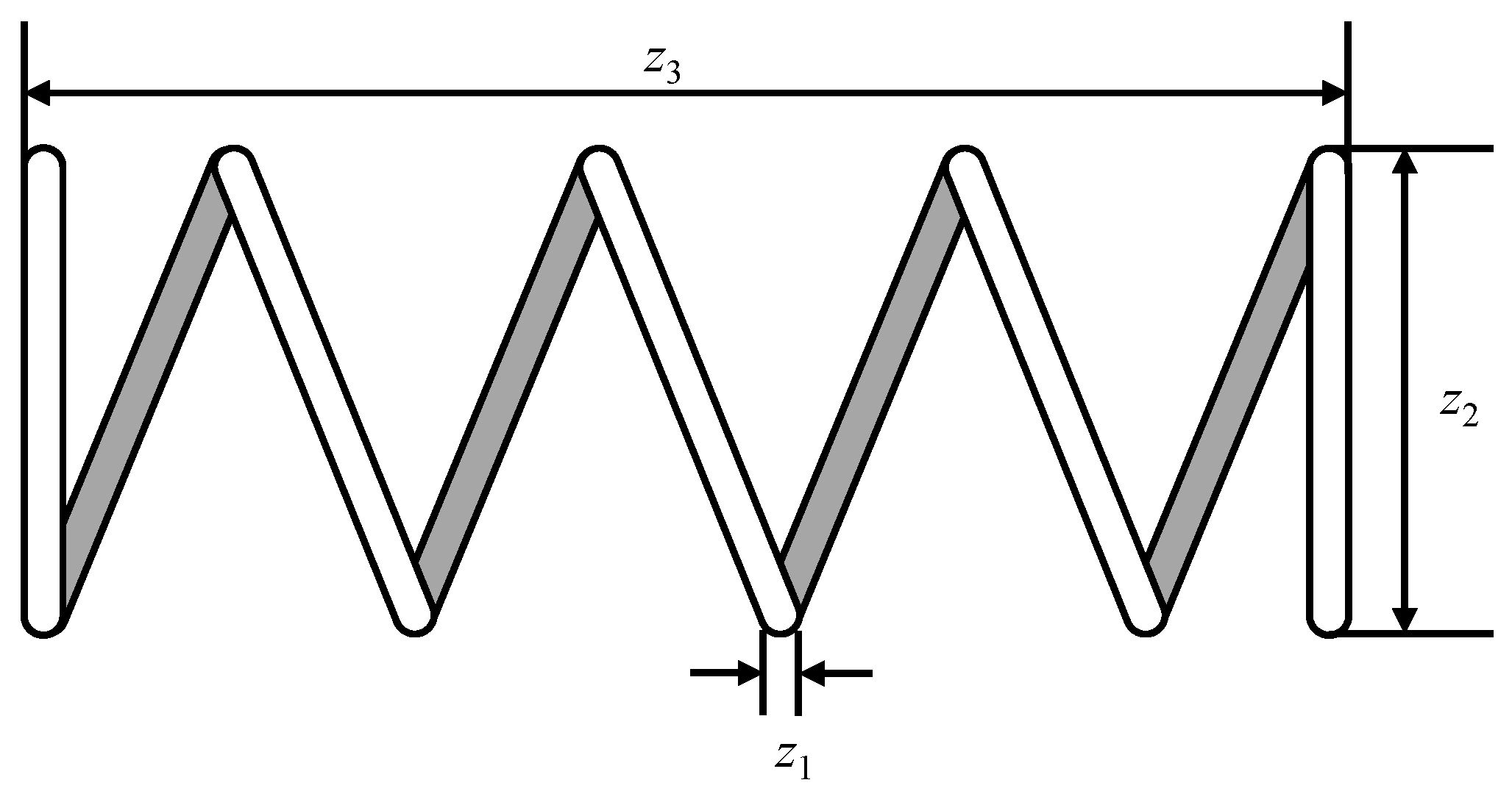
42], spring design (EA2) [43], pressure vessel design (EA3) [44], tubular column design (EA4) [45], piston lever design (EA5) [46], and reinforced concrete beam design (EA6) [47]. The second type of engineering application problem in this section is an unmanned ground vehicle (UGV) multi-target path planning problem (EA7) [48]. Different from the 58 test functions in the previous section, these engineering application problems are constrained optimization problems. To deal with the constraint conditions of these engineering application problems in a simple and efficient way, this section adopts a penalty function approach [49] as the constraint handling strategy. A detailed presentation of the aforementioned seven engineering application problems, as well as the corresponding experimental results and analysis across seven engineering application problems, is provided by the subsequent subsections.

5.1. Three-Bar Truss Design (EA1)

Figure 5 presents the first engineering application problem, which aims at minimizing the volume for three-bar truss. This problem involves optimizing two parameters while satisfying three constraints. The detailed description of solution construction, cost function, constraint conditions, and variable bounds for this three-bar truss design problem are given through Equations (23)–(27).
Solution construction:
z = [ z 1 , z 2 ] ,
Cost function:
min f EA 1 ( z ) = ( 2 2 z 1 + z 2 ) L ,
Constraint conditions:
c 1 ( z ) = 2 z 1 + z 2 2 z 1 2 + 2 z 1 z 2 P σ 0 , c 2 ( z ) = z 2 2 z 1 2 + 2 z 1 z 2 P σ 0 , c 3 ( z ) = 1 z 1 + 2 z 2 P σ 0 ,
Variable bounds:
0 z 1 1 , 0 z 2 1 ,
where
L = 100 , σ = 2 , P = 2 .

5.2. Spring Design (EA2)

Figure 6 shows the second engineering application problem, which aims at minimizing the weight for spring. The problem involves optimizing three parameters while satisfying four constraints. The detailed description of solution construction, cost function, constraint conditions, and variable bounds for this spring design problem are given through Equations (28)–(31).
Solution construction:
z = [ z 1 , z 2 , z 3 ] ,
Cost function:
min f EA 2 ( z ) = ( z 3 + 2 ) z 1 2 z 2 ,
Constraint conditions:
c 1 ( z ) = 1 z 2 3 z 3 71785 z 1 4 0 , c 2 ( z ) = 4 z 2 2 z 1 z 2 12566 ( z 1 3 z 2 z 1 4 ) + 1 5108 z 1 2 1 0 , c 3 ( z ) = 1 140.45 z 1 z 2 2 z 3 0 , c 4 ( z ) = z 1 + z 2 1.5 1 0 ,
Variable bounds:
0.05 z 1 2 , 0.25 z 2 1.3 , 2 z 3 15 .

5.3. Pressure Vessel Design (EA3)

Figure 7 presents the third engineering application problem, which aims to minimize the fabrication cost for the pressure vessel. This problem involves optimizing four parameters while satisfying four constraints. The detailed description of solution construction, cost function, constraint conditions, and variable bounds for this pressure vessel design problem are given through Equations (32)–(35).
Solution construction:
z = [ z 1 , z 2 , z 3 , z 4 ] ,
Cost function:
min f EA 3 ( z ) = 0.6224 z 1 z 3 z 4 + 19.84 z 1 2 z 3 + 1.7781 z 2 z 3 2 + 3.1661 z 1 2 z 4 ,
Constraint conditions:
c 1 ( z ) = z 1 + 0.0193 z 3 0 , c 2 ( z ) = z 2 + 0.00954 z 3 0 , c 3 ( z ) = π z 3 2 z 4 4 3 π z 3 3 + 1296000 0 , c 4 ( z ) = z 4 240 0 ,
Variable bounds:
0 z 1 99 , 0 z 2 99 , 10 z 3 200 , 10 z 4 200 .

5.4. Tubular Column Design (EA4)

Figure 8 presents the fourth engineering application problem, which aims to design a uniform column of the tubular section to carry a compressive load at minimum cost. This problem involves optimizing two parameters while satisfying six constraints. The detailed description of the solution construction, cost function, constraint conditions, and variable bounds for this tubular column design problem are given through Equations (36)–(40).
Solution construction:
z = [ z 1 , z 2 ] ,
Cost function:
min f EA 4 ( z ) = 9.8 z 1 z 2 + 2 z 1 ,
Constraint conditions:
c 1 ( z ) = P π z 1 z 2 σ y 1 0 , c 2 ( z ) = 8 P L 2 π 3 E z 1 z 2 ( z 1 2 + z 2 2 ) 1 0 , c 3 ( z ) = 2.0 z 1 1 0 , c 4 ( z ) = z 1 14 1 0 , c 5 ( z ) = 0.2 z 2 1 0 , c 6 ( z ) = z 2 0.8 1 0 ,
Variable bounds:
2 z 1 14 , 0.2 z 2 0.8 ,
where
P = 2500 , σ y = 500 , L = 250 , E = 0.85 × 10 6 .

5.5. Piston Lever Design (EA5)

Figure 9 shows the fifth engineering application problem, which aims at minimizing the oil volume when the lever of the piston is lifted up from 0° to 45° through locating the piston elements shown in the figure. The problem involves optimizing four parameters while satisfying four constraints. The detailed description of solution construction, cost function, constraint conditions, and variable bounds for this spring design problem are given through Equations (41)–(45).
Solution construction:
z = [ z 1 , z 2 , z 3 , z 4 ] ,
Cost function:
min f EA 5 ( z ) = 1 4 π z 3 2 ( L 2 L 1 ) ,
Constraint conditions:
c 1 ( z ) = Q L cos θ R F 0 , c 2 ( z ) = Q ( L z 4 ) M max 0 , c 3 ( z ) = 1.2 ( L 2 L 1 ) L 1 0 , c 4 ( z ) = z 3 2 z 2 0 ,
Variable bounds:
0.05 z 1 500 , 0.05 z 2 500 , 0.05 z 3 500 , 0.05 z 4 120 ,
where
R = z 4 z 4 sin θ + z 1 + z 1 z 2 z 4 cos θ z 4 z 2 2 + z 1 2 , F = π P z 3 2 4 , L 1 = z 4 z 2 2 + z 1 2 , L 2 = z 4 sin θ + z 1 2 + z 2 z 4 cos θ 2 , θ = 45 , Q = 10,000 , L = 240 , M max = 1.8 × 10 6 , P = 1500 .

5.6. Reinforced Concrete Beam Design (EA6)

Figure 10 presents the sixth engineering application problem, which aims at minimizing the total cost of the structure shown in the figure. This problem involves optimizing three parameters while satisfying two constraints. The detailed description of solution construction, cost function, constraint conditions, and variable bounds for this pressure vessel design problem are given through Equations (46)–(49).
Solution construction:
z = [ z 1 , z 2 , z 3 ] ,
Cost function:
min f EA 6 ( z ) = 2.9 z 1 + 0.6 z 2 z 3 ,
Constraint conditions:
c 1 ( z ) = z 2 z 3 4 0 , c 2 ( z ) = 180 + 7.375 z 1 2 z 3 z 1 z 2 0 ,
Variable bounds:
z 1 { 6 , 6.16 , 6.32 , 6.6 , 7 , 7.11 , 7.2 , 7.8 , 7.9 , 8 , 8.4 } , z 2 { 28 , 29 , 30 , , 40 } , 5 z 3 10 ,

5.7. UGV Multi-Target Path Planning (EA7)

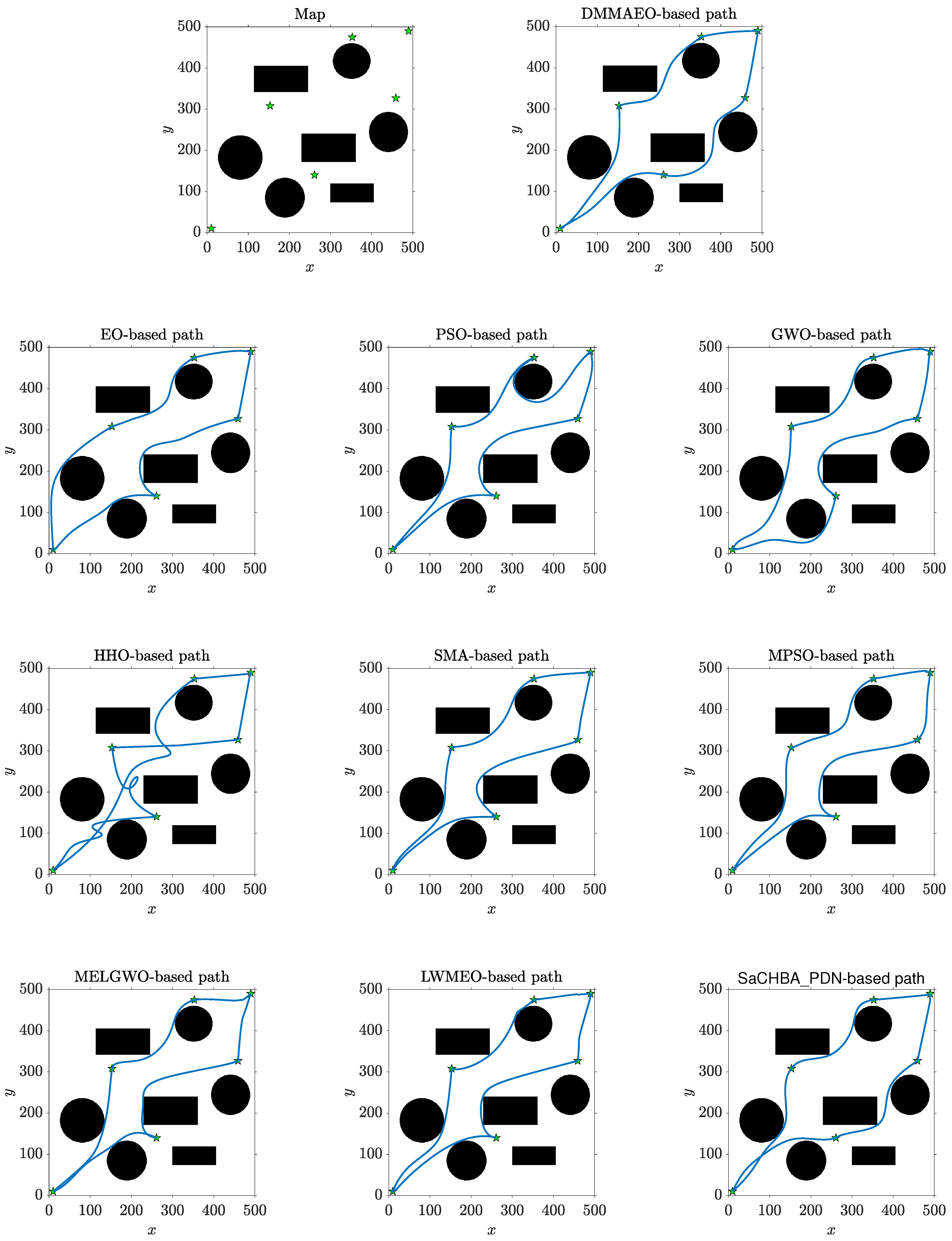
The fourth engineering application problem used in this section is the UGV multi-target path planning problem, which is common in tasks such as warehousing logistics, data collection, and security patrols. A map for the multi-target path planning problem is shown in Figure 11, where the black area represents the infeasible region formed by different types of obstacles, the white area represents the feasible region, and the pentagrams represent the multiple predefined targets. For this problem, the UGV needs to start from one of the multiple predefined targets, navigate sequentially through a series of predefined targets while avoiding obstacles, stop at each predefined target to perform the corresponding task operation, and finally return to the starting location. Therefore, this problem aims to obtain the shortest feasible path for the UGV through multiple predefined targets in an obstacle environment so as to achieve the efficient processing of related tasks. The detailed description of the mathematical model for this UGV multi-target path planning problem are given through Equation (50).
min f EA 7 ( Q ) = k = 1 K Q k ,
s . t .   Q O b ,
where Q represents the total path connecting all predefined targets in turn, which consists of a series of path points ( Q x , Q y ) ; K is the overall amount for sub-paths, which is also the same as the overall amount for predefined targets; Q k denotes the path length for the k-th sub-path in the total path; and O b represents the infeasible region in the obstacle environment.
In accordance with the features from the UGV multi-target path planning problem, the problem can be transformed into two types of sub-problems: a path planning problem between any two predefined targets and a traveling salesman problem. In this way, the optimal solution of path planning problem between any two predefined targets yields the shortest path between any two predefined targets. Then, based on the results of the shortest path between any two predefined targets, the optimal solution of traveling salesman problem yields the shortest total path through all predefined targets.
In addition, a smooth path is helpful for the subsequent tracking control of UGV to avoid unnecessary overdriving and slipping. For this purpose, the cubic quasi-uniform B-spline curve approach is applied to generate the smooth path for the UGV multi-target path planning problem, which can guarantee driveability and smoothness for the generated path [50]. The B-spline curve is constructed through
Q ( t ) = l = 0 L F l , m ( t ) q l , l = 0 , 1 , , L ,
where Q ( t ) indicates the B-spline curve; m is the order of B-spline curve, and the corresponding degree of B-spline curve is m 1 ; the overall control points amount is L + 1 , which needs to be greater than or equal to the order m; q l represents the ( l + 1 ) -th control point of B-spline curve; F l , m ( t ) indicates the B-spline basic function with m-order for ( l + 1 ) -th control point, which is calculated through Cox-de Boor recursion formulas as
F l , m ( t ) = 1 , t l t < t l + 1 0 , otherwise , m = 1 , F l , m ( t ) = t t l t l + m 1 t l F l , m 1 ( t ) + t l + m t t l + m t l + 1 F l + 1 , m 1 ( t ) , m 2 ,
where ‛ 0 / 0 = 0 ’ is defined in Equation (53); and the B-spline basic function is formed through a non-decreasing sequence with continuously varying values { t 0 , t 1 , , t n + k } called the knot vector, whose values at the beginning and end are commonly fixed at 0 and 1, respectively. For a cubic quasi-uniform B-spline curve, the degree needs to be set at 3, the knots at both ends in the knot vector have a repetition of 4, and the middle knots are uniformly distributed. So when the order m is set to 4 and the distribution of the knot vector is set according to the previous requirements, the cubic quasi-uniform B-spline curve can be obtained to generate the smooth path. The cubic quasi-uniform B-spline curve can generate a smooth path through the determination of several control points, the generated path passes through the first and last control points, and the adjustment of individual control points can locally modify the generated path. These characteristics make the cubic quasi-uniform B-spline curve suitable for generating smooth paths and effectively improve the computational efficiency. Additionally, the UGV in the multi-target path planning problem needs to stop at each predefined target to perform the corresponding task operation. So, the cubic quasi-uniform B-spline curve approach is only required to generate a smooth path between any two predefined targets, and there is no need to ensure smoothness for the total path at each target.
With the combination of the cubic quasi-uniform B-spline curve approach and the proposed DMMAEO, the steps involved in solving multi-target path planning problem are shown below:
Step 1 Set the elements associated with multi-target path planning problem such as map M a p , order m and number of control points L + 1 in each sub-path, and the predefined multiple targets denoted by q 0 and q M in each sub-path.
Step 2 Set the related parameters for DMMAEO, including current iteration number g, maximum iteration number g max , population size N, particle dimension L + 1 as per number of control points, sub-population number M, and reorganization period R p .
Step 3 Set the cost function of DMMAEO according to Equation (50).
Step 4 Initialize the control points using the DMMAEO concentration initialization mechanism and calculate the cost function of the corresponding initial sub-path generated by the cubic quasi-uniform B-spline curve between any two predefined targets.
Step 5 Optimize the control point positions in each sub-path based on the DMMAEO to find the shortest sub-path between any two predefined targets.
Step 6 Run Step 5 until the termination condition specified by this path planning sub-problem between any two predefined targets is satisfied.
Step 7 Based on the shortest sub-path between any two predefined targets, calculate the cost function of the total paths connecting all predefined targets generated by the random keys technology [51].
Step 8 Optimize the connection sequence of each sub-path in the total path based on the DMMAEO to find the shortest total path through all predefined targets.
Step 9 Run Step 8 until the termination condition specified by this traveling salesman sub-problem is satisfied.
Step 10 Return the shortest total path through all predefined targets for the multi-target path planning.

5.8. Results and Analysis of DMMAEO on Engineering Application Problems

For examining the practicability of DMMAEO, the seven engineering application problems (EA1-EA7) mentioned above are solved by the DMMAEO in this subsection, which are also solved by several recent promising algorithms with three categories mentioned in the previous section (EO [11], PSO [8], GWO [5], HHO [6], SMA [7], MPSO [36], MELGWO [37], LWMEO [20], SASS [52], and SaCHBA_PDN [53]) for comparison. Among the compared algorithms, SASS is the best algorithm for addressing engineering optimization problem, and SaCHBA_PDN is the best algorithm for addressing the path planning problem. Similar to the previous section, the compared algorithms adopt identical experimental settings to ensure the fairness of optimization performance comparison in solving engineering application problems. In this section, the best fitness value (Best), average fitness value (Ave.), worst fitness value (Worst), and standard deviation of fitness value (Std.) are applied in assessing the algorithm performance. Table 15, Table 16, Table 17, Table 18, Table 19, Table 20 and Table 21 show the results for the compared algorithms, which are obtained by implementing each algorithm 30 times independently on each engineering application problem. In Table 15, Table 16, Table 17, Table 18, Table 19, Table 20 and Table 21, the best results and the top-performing algorithm are highlighted in bold.
As per the results of the three-bar truss design (EA1) from Table 15, the DMMAEO exhibits a superior performance compared to the other algorithms in minimizing the volume of three-bar truss. Regarding the spring design (EA2), the DMMAEO achieves the strongest performance in minimizing the spring weight compared to other algorithms based on the results from Table 16. Regarding the pressure vessel design (EA3), the DMMAEO outperforms the compared algorithms in terms of minimizing the fabrication cost of the pressure vessel based on the results from Table 17. As per the results of the tubular column design (EA4) from 
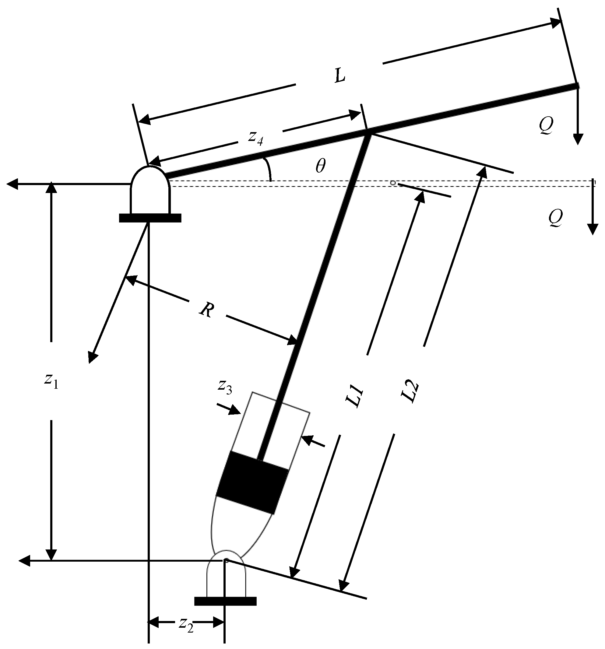
Table 18, the DMMAEO exhibits a superior performance compared to the other algorithms in designing a uniform column of the tubular section to carry a compressive load at minimum cost. Regarding the piston lever design (EA5), the DMMAEO achieves the strongest performance in minimizing the oil volume when the lever of the piston is lifted up from 0° to 45° compared to the other algorithms based on the results from 
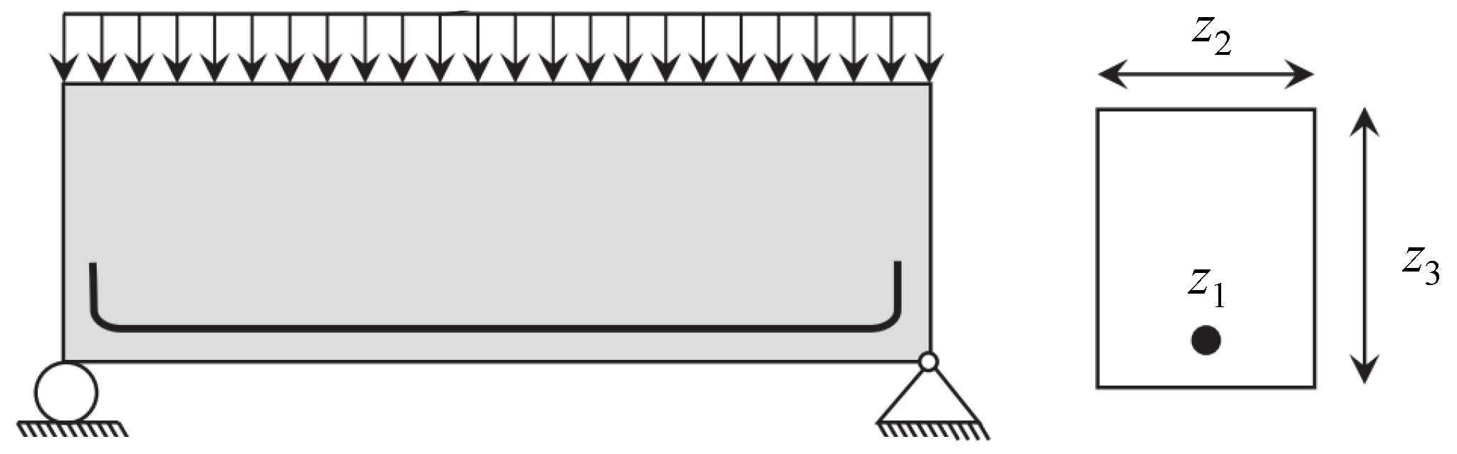
Table 19. Regarding the reinforced concrete beam design (EA6), the DMMAEO outperforms the compared algorithms in terms of minimizing the total cost of the structure based on the results from Table 20. As per the results of UGV multi-target path planning problem (EA7) in Figure 11 and Table 21, the compared algorithms generate feasible paths in different types and the DMMAEO performs better in obtaining the shortest path compared to other algorithms. Therefore, the DMMAEO outperforms other compared algorithms and obtains the top rank in all seven engineering application problems. These results mean that the DMMAEO is superior to other compared algorithms and exhibits the most competitive overall performance within the compared algorithms for addressing engineering application problems. Based on the aforementioned results, it can be seen that the DMMAEO efficiently solves the engineering application problem by constructing dynamic multi-population mutation architecture. In the UGV multi-target path planning problem (EA7) especially, the dynamic multi-population mutation architecture in the DMMAEO could effectively deal with the problems caused by various obstacles, multi-stage optimization, and numerous local optima through enhancing population diversity and search ability, which makes the DMMAEO more suitable for the UGV multi-target path planning problem.
To summarize, the results and analysis mentioned above indicate that the proposed DMMAEO has practicability and competitiveness in solving engineering application problems.

6. Conclusions

A dynamic multi-population mutation architecture-based equilibrium optimizer (DMMAEO) is developed for strengthening the population diversity and search capability of the canonical equilibrium optimizer (EO). In the DMMAEO, a dynamic multi-population guidance mechanism is introduced to construct a sub-population structure and corresponding information interaction mode, which can increase the population diversity. Moreover, a dynamic Gaussian mutation-based sub-population concentration updating mechanism is integrated to use the neighborhood space information of sub-population particle concentrations, which can strengthen the exploitation ability. Finally, a dynamic Cauchy mutation-based sub-population equilibrium candidate generation mechanism is constructed in order to employ the promising space information of sub-population equilibrium candidates, which can improve the exploration ability.
For investigating the effectiveness of the three enhancement mechanisms from DMMAEO, the DMMAEO and different EO variants constructed by the three enhancement mechanisms are conducted on the 29 representative test functions. The test experiment results indicate that all three enhancement mechanisms are effective in enhancing the performance of the canonical EO, and the DMMAEO performs best among the different EO variants. Then, the DMMAEO is further compared with several recent promising algorithms on 58 test functions to analyze the superiority of DMMAEO. According to the comparative results of the performance assessment, the DMMAEO performs better optimization performance than the compared algorithms and achieves the top rank. In addition, the DMMAEO is utilized for tackling six engineering design problems and a UGV multi-target path planning problem, which are also solved by several recent promising algorithms for comparison. The results of the engineering application experiments denote that the DMMAEO has practicability and competitiveness in solving engineering application problems. To summarize, the dynamic multi-population mutation architecture in the DMMAEO enhances the optimization ability of the canonical EO via effectively constructing sub-population structure and using sub-population information, which makes it more effective than other algorithms. Moreover, the DMMAEO offers an effective method for tackling complex numerical optimization and engineering application challenges. Meanwhile, the average running time of DMMAEO is slightly higher than other compared algorithms, but better than the top algorithm EBOwithCMAR. Therefore, if accuracy is the main objective of solving optimization problems, the DMMAEO is a competitive and acceptable high performance optimizer.
Regarding future work, the DMMAEO will be further developed to reduce its running time while maintaining its superior optimization performance. Moreover, designing the extended forms of DMMAEO to deal with the discrete and multi-objective optimization problems is also a noteworthy investigation. Additionally, the DMMAEO is expected to handle more types of practical application problems, such as medical diagnosis, financial stress prediction, structural damage identification, wireless sensor network coverage, and so on.

Author Contributions

Conceptualization, X.W.; methodology, X.W.; validation, X.W. and S.S.; investigation, Y.D.; writing—original draft preparation, X.W.; writing—review and editing, K.H. and Y.D.; supervision, K.H. and Y.D.; project administration, K.H and S.S. All authors have read and agreed to the published version of the manuscript.

Funding

This research was funded in part by the National Natural Science Foundation of China under Grant No.82201753 and in part by the Systematic Major Project of China Railway Group under Grant No. P2021T002.

Institutional Review Board Statement

Not applicable.

Informed Consent Statement

Not applicable.

Data Availability Statement

The original contributions presented in the study are included in the article; further inquiries can be directed to the corresponding author.

Conflicts of Interest

The authors declare no conflicts of interest.

References

  1. Zhang, Y.Y.; Liu, L.S.; Liang, J.R.; Chen, J.H.; Ke, C.Y.; He, D.W. Application of a Multi-Strategy Improved Sparrow Search Algorithm in Bridge Crane PID Control Systems. Appl. Sci. 2024, 14, 5165. [Google Scholar] [CrossRef]
  2. Li, Y.H.; Zhang, T.Y.; Yu, X.T.; Sun, F.H.; Liu, P.Z.; Zhu, K. Research on Agricultural Product Price Prediction Based on Improved PSO-GA. Appl. Sci. 2024, 14, 6862. [Google Scholar] [CrossRef]
  3. Luo, J.; Chen, H.L.; Zhang, Q.; Xu, Y.T.; Huang, H.; Zhao, X.H. An improved grasshopper optimization algorithm with application to financial stress prediction. Appl. Math. Model. 2018, 64, 654–668. [Google Scholar] [CrossRef]
  4. Li, Z.F.; Zeng, J.H.; Chen, Y.Q.; Ma, G.; Liu, G.Y. Death mechanism-based moth–flame optimization with improved flame generation mechanism for global optimization tasks. Expert Syst. Appl. 2021, 183, 115436. [Google Scholar] [CrossRef]
  5. Faris, H.; Aljarah, I.; Al-Betar, M.A.; Mirjalili, S. Grey wolf optimizer: A review of recent variants and applications. Neural Comput. Appl. 2018, 30, 413–435. [Google Scholar] [CrossRef]
  6. Alabool, H.M.; Alarabiat, D.; Abualigah, L.; Heidari, A.A. Harris hawks optimization: A comprehensive review of recent variants and applications. Neural Comput. Appl. 2021, 33, 8939–8980. [Google Scholar] [CrossRef]
  7. Gharehchopogh, F.S.; Ucan, A.; Ibrikci, T.; Arasteh, B.; Isik, G. Slime mould algorithm: A comprehensive survey of its variants and applications. Arch. Comput. Methods Eng. 2023, 30, 2683–2723. [Google Scholar] [CrossRef] [PubMed]
  8. Houssein, E.H.; Gad, A.G.; Hussain, K.; Suganthan, P.N. Major advances in particle swarm optimization: Theory, analysis, and application. Swarm Evol. Comput. 2021, 63, 100868. [Google Scholar] [CrossRef]
  9. Dehghani, M.; Mardaneh, M.; Guerrero, J.M.; Malik, O.P.; Ramirez-Mendoza, R.A.; Matas, J.; Vasquez, J.C.; Parra-Arroyo, L. A new “Doctor and Patient” optimization algorithm: An application to energy commitment problem. Appl. Sci. 2020, 10, 5791. [Google Scholar] [CrossRef]
  10. Joyce, T.; Herrmann, J.M. A review of no free lunch theorems, and their implications for metaheuristic optimisation. In Nature-Inspired Algorithms and Applied Optimization; Springer: Cham, Switzerland, 2018; pp. 27–51. [Google Scholar]
  11. Faramarzi, A.; Heidarinejad, M.; Stephens, B.; Mirjalili, S. Equilibrium optimizer: A novel optimization algorithm. Knowl. Based Syst. 2020, 191, 105190. [Google Scholar] [CrossRef]
  12. Nusair, K.; Alhmoud, L. Application of equilibrium optimizer algorithm for optimal power flow with high penetration of renewable energy. Energies 2020, 13, 6066. [Google Scholar] [CrossRef]
  13. Nguyen, T.; Nguyen, G.; Nguyen, B.M. EO-CNN: An enhanced CNN model trained by equilibrium optimization for traffic transportation prediction. Procedia Comput. Sci. 2020, 176, 800–809. [Google Scholar] [CrossRef]
  14. Wu, X.D.; Hirota, K.; Tang, B.J.; Dai, Y.P.; Jia, Z.Y. Ameliorated Frenet trajectory optimization method based on artificial emotion and equilibrium optimizer. J. Adv. Comput. Intell. 2021, 25, 110–120. [Google Scholar] [CrossRef]
  15. Dinh, P.H. Multi-modal medical image fusion based on equilibrium optimizer algorithm and local energy functions. Appl. Intell. 2021, 51, 8416–8431. [Google Scholar] [CrossRef]
  16. Elsheikh, A.H.; Shehabeldeen, T.A.; Zhou, J.X.; Showaib, E.; Abd Elaziz, M. Prediction of laser cutting parameters for polymethylmethacrylate sheets using random vector functional link network integrated with equilibrium optimizer. J. Intell. Manuf. 2021, 32, 1377–1388. [Google Scholar] [CrossRef]
  17. Abdel-Basset, M.; Mohamed, R.; Mirjalili, S.; Chakrabortty, R.K.; Ryan, M.J. Solar photovoltaic parameter estimation using an improved equilibrium optimizer. Sol. Energy 2020, 209, 694–708. [Google Scholar] [CrossRef]
  18. Naik, M.K.; Panda, R.; Abraham, A. An opposition equilibrium optimizer for context-sensitive entropy dependency based multilevel thresholding of remote sensing images. Swarm Evol. Comput. 2021, 65, 100907. [Google Scholar] [CrossRef]
  19. Too, J.W.; Mirjalili, S. General learning equilibrium optimizer: A new feature selection method for biological data classification. Appl. Artif. Intell. 2021, 35, 247–263. [Google Scholar] [CrossRef]
  20. Liu, J.S.; Li, W.X.; Li, Y. LWMEO: An efficient equilibrium optimizer for complex functions and engineering design problems. Expert Syst. Appl. 2022, 198, 116828. [Google Scholar] [CrossRef]
  21. Wu, X.D.; Hirota, K.; Jia, Z.Y.; Ji, Y.; Zhao, K.X.; Dai, Y.P. Ameliorated equilibrium optimizer with application in smooth path planning oriented unmanned ground vehicle. Knowl.-Based Syst. 2023, 260, 110148. [Google Scholar] [CrossRef]
  22. Ma, H.P.; Shen, S.G.; Yu, M.; Yang, Z.L.; Fei, M.R.; Zhou, H.Y. Multi-population techniques in nature inspired optimization algorithms: A comprehensive survey. Swarm Evol. Comput. 2019, 44, 365–387. [Google Scholar] [CrossRef]
  23. Xia, X.W.; Gui, L.; Zhan, Z.H. A multi-swarm particle swarm optimization algorithm based on dynamical topology and purposeful detecting. Appl. Soft Comput. 2018, 67, 126–140. [Google Scholar] [CrossRef]
  24. Sun, Y.J.; Chen, Y. Multi-population improved whale optimization algorithm for high dimensional optimization. Appl. Soft Comput. 2021, 112, 107854. [Google Scholar] [CrossRef]
  25. Saha, A.K. Multi-population-based adaptive sine cosine algorithm with modified mutualism strategy for global optimization. Knowl.-Based Syst. 2022, 251, 109326. [Google Scholar] [CrossRef]
  26. Yu, F.; Guan, J.; Wu, H.R.; Wang, H.; Ma, B.Y. Multi-population differential evolution approach for feature selection with mutual information ranking. Expert Syst. Appl. 2025, 260, 125404. [Google Scholar] [CrossRef]
  27. Liu, J.; Ma, D.; Ma, T.B.; Zhang, W. Ecosystem particle swarm optimization. Soft Comput. 2017, 21, 1667–1691. [Google Scholar] [CrossRef]
  28. Chen, K.; Xue, B.; Zhang, M.J.; Zhou, F.Y. Novel chaotic grouping particle swarm optimization with a dynamic regrouping strategy for solving numerical optimization tasks. Knowl. Based Syst. 2020, 194, 105568. [Google Scholar] [CrossRef]
  29. Chen, K.; Zhou, F.Y.; Yuan, X.F. Hybrid particle swarm optimization with spiral-shaped mechanism for feature selection. Expert Syst. Appl. 2019, 128, 140–156. [Google Scholar] [CrossRef]
  30. Liu, Y.; Heidari, A.A.; Cai, Z.N.; Liang, G.X.; Chen, H.L.; Pan, Z.F.; Alsufyani, A.; Bourouis, S. Simulated annealing-based dynamic step shuffled frog leaping algorithm: Optimal performance design and feature selection. Neurocomputing 2022, 503, 325–362. [Google Scholar] [CrossRef]
  31. Ma, C.; Huang, H.S.; Fan, Q.S.; Wei, J.N.; Du, Y.M.; Gao, W.S. Grey wolf optimizer based on Aquila exploration method. Expert Syst. Appl. 2022, 205, 117629. [Google Scholar] [CrossRef]
  32. Shami, T.M.; Mirjalili, S.; Al-Eryani, Y.; Daoudi, K.; Izadi, S.; Abualigah, L. Velocity pausing particle swarm optimization: A novel variant for global optimization. Neural Comput. Appl. 2023, 35, 9193–9223. [Google Scholar] [CrossRef]
  33. Wang, Y.; Ran, S.J.; Wang, G.G. Role-oriented binary grey wolf optimizer using foraging-following and Lévy flight for feature selection. Appl. Math. Model. 2024, 126, 310–326. [Google Scholar] [CrossRef]
  34. Zhong, C.T.; Li, G.; Meng, Z. Beluga whale optimization: A novel nature-inspired metaheuristic algorithm. Knowl.Based Syst. 2022, 251, 109215. [Google Scholar] [CrossRef]
  35. Faramarzi, A.; Heidarinejad, M.; Mirjalili, S.; Gandomi, A.H. Marine Predators Algorithm: A nature-inspired metaheuristic. Expert Syst. Appl. 2020, 152, 113377. [Google Scholar] [CrossRef]
  36. Liu, H.; Zhang, X.W.; Tu, L.P. A modified particle swarm optimization using adaptive strategy. Expert Syst. Appl. 2020, 152, 113353. [Google Scholar] [CrossRef]
  37. Ahmed, R.; Rangaiah, G.P.; Mahadzir, S.; Mirjalili, S.; Hassan, M.H.; Kamel, S. Memory, evolutionary operator, and local search based improved Grey Wolf Optimizer with linear population size reduction technique. Knowl.Based Syst. 2023, 264, 110297. [Google Scholar] [CrossRef]
  38. Kumar, A.; Misra, R.K.; Singh, D. Improving the local search capability of effective butterfly optimizer using covariance matrix adapted retreat phase. In Proceedings of the 2017 IEEE Congress on Evolutionary Computation (CEC), Donostia, Spain, 5–8 June 2017; IEEE: Piscataway, NJ, USA, 2017; pp. 1835–1842. [Google Scholar]
  39. Zhao, X.D.; Fang, Y.M.; Liu, L.; Xu, M.; Li, Q. A covariance-based Moth–flame optimization algorithm with Cauchy mutation for solving numerical optimization problems. Appl. Soft Comput. 2022, 119, 108538. [Google Scholar] [CrossRef]
  40. Nadimi-Shahraki, M.H.; Taghian, S.; Mirjalili, S. An improved grey wolf optimizer for solving engineering problems. Expert Syst. Appl. 2021, 166, 113917. [Google Scholar] [CrossRef]
  41. Cheng, S.; Shi, Y.H.; Qin, Q.D.; Zhang, Q.Y.; Bai, R.B. Population diversity maintenance in brain storm optimization algorithm. J. Artif. Intell. Soft 2014, 4, 83–97. [Google Scholar] [CrossRef]
  42. Chopra, N.; Ansari, M.M. Golden jackal optimization: A novel nature-inspired optimizer for engineering applications. Expert Syst. Appl. 2022, 198, 116924. [Google Scholar] [CrossRef]
  43. Heidari, A.A.; Mirjalili, S.; Faris, H.; Aljarah, I.; Mafarja, M.; Chen, H.L. Harris hawks optimization: Algorithm and applications. Future Gener. Comput. Syst. 2019, 97, 849–872. [Google Scholar] [CrossRef]
  44. Luo, J.; Chen, H.; Heidari, A.A.; Xu, Y.; Zhang, Q.; Li, C. Multi-strategy boosted mutative whale-inspired optimization approaches. Appl. Math. Model. 2019, 73, 109–123. [Google Scholar] [CrossRef]
  45. Che, Y.; He, D. An enhanced seagull optimization algorithm for solving engineering optimization problems. Appl. Intell. 2022, 52, 13043–13081. [Google Scholar] [CrossRef]
  46. Kumar, S.; Yildiz, B.S.; Mehta, P.; Panagant, N.; Sait, S.M.; Mirjalili, S.; Yildiz, A.R. Chaotic marine predators algorithm for global optimization of real-world engineering problems. Knowl.Based Syst. 2023, 261, 110192. [Google Scholar] [CrossRef]
  47. Amir, H.M.; Hasegawa, T. Nonlinear mixed-discrete structural optimization. J. Struct. Eng. 1989, 115, 626–646. [Google Scholar] [CrossRef]
  48. Lv, Q.; Yang, D. Multi-target path planning for mobile robot based on improved PSO algorithm. In Proceedings of the 2020 IEEE 5th Information Technology and Mechatronics Engineering Conference (ITOEC), Chongqing, China, 12–14 June 2020; IEEE: Piscataway, NJ, USA, 2020; pp. 1042–1047. [Google Scholar]
  49. Talbi, E.G. Metaheuristics: From Design to Implementation; John Wiley & Sons: Hoboken, NJ, USA, 2009. [Google Scholar]
  50. Wang, P.W.; Yang, J.S.; Zhang, Y.L.; Wang, Q.W.; Sun, B.B.; Guo, D. Obstacle-Avoidance Path-Planning Algorithm for Autonomous Vehicles Based on B-Spline Algorithm. World Electr. Veh. J. 2022, 13, 233. [Google Scholar] [CrossRef]
  51. Osaba, E.; Villar-Rodriguez, E.; Del Ser, J.; Nebro, A.J.; Molina, D.; LaTorre, A.; Suganthan, P.N.; Coello, C.A.C.; Herrera, F. A tutorial on the design, experimentation and application of metaheuristic algorithms to real-world optimization problems. Swarm Evol. Comput. 2021, 64, 100888. [Google Scholar] [CrossRef]
  52. Kumar, A.; Das, S.; Zelinka, I. A self-adaptive spherical search algorithm for real-world constrained optimization problems. In Proceedings of the 2020 Genetic and Evolutionary Computation Conference Companion, Cancún Mexico, 8–12 July 2020; pp. 13–14. [Google Scholar]
  53. Hu, G.; Zhong, J.Y.; Wei, G. SaCHBA_PDN: Modified honey badger algorithm with multi-strategy for UAV path planning. Expert Syst. Appl. 2023, 223, 119941. [Google Scholar] [CrossRef]
Figure 1. Flowchart of DMMAEO.
Applsci 15 01795 g001
Figure 2. Convergence curves for canonical EO and four EO variants across 9 test functions.
Applsci 15 01795 g002
Figure 3. Diversity curves across 9 test functions.
Applsci 15 01795 g003
Figure 4. Convergence curves for DMMAEO and several recent promising algorithms across 9 test functions.
Applsci 15 01795 g004
Figure 5. Three-bar truss design.
Applsci 15 01795 g005
Figure 6. Spring design.
Applsci 15 01795 g006
Figure 7. Pressure vessel design.
Applsci 15 01795 g007
Figure 8. Tubular column design.
Applsci 15 01795 g008
Figure 9. Piston lever design.
Applsci 15 01795 g009
Figure 10. Reinforced concrete beam design.
Applsci 15 01795 g010
Figure 11. Multi-target path planning results of compared algorithms.
Applsci 15 01795 g011
Table 1. Results for canonical EO and four EO variants across unimodal test functions.
Function EODMEOGMEOCMEODMMAEO
UnimodalTF1Ave. 4.297 × 10 41 4.757 × 10 63 0.000 × 10 0 3.995 × 10 148 0 . 000 × 10 0
Std. 7.488 × 10 41 5.266 × 10 63 0.000 × 10 0 1.727 × 10 147 0.000 × 10 0
TF2Ave. 1.494 × 10 23 3.743 × 10 37 1.719 × 10 232 4.031 × 10 77 2 . 614 × 10 308
Std. 2.772 × 10 23 2.931 × 10 37 0.000 × 10 0 1.185 × 10 76 0.000 × 10 0
TF3Ave. 9.458 × 10 9 2.183 × 10 14 0.000 × 10 0 7.093 × 10 133 0 . 000 × 10 0
Std. 3.193 × 10 8 3.969 × 10 14 0.000 × 10 0 3.859 × 10 132 0.000 × 10 0
TF4Ave. 3.885 × 10 10 3.016 × 10 11 3.448 × 10 227 3.243 × 10 71 2 . 164 × 10 304
Std. 5.952 × 10 10 3.166 × 10 11 0.000 × 10 0 1.520 × 10 70 0.000 × 10 0
TF5Ave. 2.544 × 10 1 2.505 × 10 1 2.513 × 10 1 2.536 × 10 1 2 . 469 × 10 1
Std. 1.393 × 10 1 1.028 × 10 1 9.691 × 10 2 1.551 × 10 1 1.189 × 10 1
TF6Ave. 1.262 × 10 5 4.302 × 10 6 7.355 × 10 6 7.908 × 10 6 1 . 437 × 10 6
Std. 7.772 × 10 6 1.554 × 10 6 3.143 × 10 6 3.089 × 10 6 5.836 × 10 7
TF7Ave. 1.633 × 10 3 9.423 × 10 4 8.868 × 10 4 9.406 × 10 4 4 . 582 × 10 5
Std. 6.363 × 10 4 3.459 × 10 4 3.900 × 10 4 3.063 × 10 4 3.313 × 10 5
The best comparative results are presented in bold.
Table 2. Results for canonical EO and four EO variants across multimodal test functions with high dimension.
Function EODMEOGMEOCMEODMMAEO
Multimodal (High dimension)TF8Ave. 8.586 × 10 3 8.753 × 10 3 8.973 × 10 3 9.032 × 10 3 9 . 152 × 10 3
Std. 3.178 × 10 2 3.509 × 10 2 4.903 × 10 2 3.744 × 10 2 7.372 × 10 2
TF9Ave. 0.000 × 10 0 0.000 × 10 0 0.000 × 10 0 0.000 × 10 0 0 . 000 × 10 0
Std. 0.000 × 10 0 0.000 × 10 0 0.000 × 10 0 0.000 × 10 0 0.000 × 10 0
TF10Ave. 1.036 × 10 14 8.882 × 10 16 8.882 × 10 16 8.882 × 10 16 8 . 882 × 10 16
Std. 3.407 × 10 15 0.000 × 10 0 0.000 × 10 0 0.000 × 10 0 0.000 × 10 0
TF11Ave. 0.000 × 10 0 0.000 × 10 0 0.000 E × 10 0 0.000 × 10 0 0 . 000 × 10 0
Std. 0.000 × 10 0 0.000 × 10 0 0.000 × 10 0 0.000 × 10 0 0.000 × 10 0
TF12Ave. 8.485 × 10 7 2.619 × 10 7 5.072 × 10 7 4.565 × 10 7 1 . 080 × 10 7
Std. 6.308 × 10 7 9.046 × 10 8 3.348 × 10 7 1.858 × 10 7 4.348 × 10 8
TF13Ave. 5.414 × 10 2 2 . 498 × 10 2 2.276 × 10 0 4.093 × 10 1 3.486 × 10 1
Std. 5.411 × 10 2 3.745 × 10 2 4.355 × 10 1 4.493 × 10 1 2.149 × 10 1
The best comparative results are presented in bold.
Table 3. Results for canonical EO and four EO variants across multimodal test functions with fixed dimension.
Function EODMEOGMEOCMEODMMAEO
Multimodal (Fixed-dimension)TF14Ave. 9.980 × 10 1 9.980 × 10 1 4.388 × 10 0 9.980 × 10 1 9 . 980 × 10 1
Std. 1.934 × 10 16 0.000 × 10 0 4.457 × 10 0 1.797 × 10 16 0.000 × 10 0
TF15Ave. 5.916 × 10 3 3.077 × 10 4 2.417 × 10 3 5.122 × 10 3 3 . 075 × 10 4
Std. 8.869 × 10 3 3.206 × 10 7 6.091 × 10 3 8.557 × 10 3 7.765 × 10 9
TF16Ave. 1.032 × 10 0 1.032 × 10 0 1.032 × 10 0 1.032 × 10 0 1 . 032 × 10 0
Std. 5.904 × 10 16 6.775 × 10 16 5.904 × 10 16 5.831 × 10 16 6.775 × 10 16
TF17Ave. 3.979 × 10 1 3.979 × 10 1 3.979 × 10 1 3.979 × 10 1 3 . 979 × 10 1
Std. 0.000 × 10 0 0.000 × 10 0 0.000 × 10 0 0.000 × 10 0 0.000 × 10 0
TF18Ave. 3.000 × 10 0 3.000 × 10 0 3.000 × 10 0 3.000 × 10 0 3 . 000 × 10 0
Std. 1.195 × 10 15 1.641 × 10 15 1.215 × 10 15 1.189 × 10 15 1.698 × 10 15
TF19Ave. 3.863 × 10 0 3.863 × 10 0 3.863 × 10 0 3.863 × 10 0 3 . 863 × 10 0
Std. 2.437 × 10 15 2.710 × 10 15 2.294 × 10 15 2.372 × 10 15 2.710 × 10 15
TF20Ave. 3.202 × 10 0 3.322 × 10 0 3.242 × 10 0 3.243 × 10 0 3 . 322 × 10 0
Std. 3.956 × 10 2 1.424 × 10 15 6.998 × 10 2 5.715 × 10 2 1.489 × 10 15
TF21Ave. 8.465 × 10 0 1.015 × 10 1 1.015 × 10 1 1.015 × 10 1 1 . 015 × 10 1
Std. 2.681 × 10 0 1.603 × 10 4 1.565 × 10 4 5.186 × 10 5 7.196 × 10 6
TF22Ave. 9.650 × 10 0 1.040 × 10 1 1.040 × 10 1 1.040 × 10 1 1 . 040 × 10 1
Std. 1.965 × 10 0 3.239 × 10 5 1.032 × 10 4 8.418 × 10 5 7.412 × 10 6
TF23Ave. 9.369 × 10 0 1.036 × 10 1 1.054 × 10 1 1.054 × 10 1 1 . 054 × 10 1
Std. 2.392 × 10 0 9.873 × 10 1 8.811 × 10 5 4.123 × 10 5 6.438 × 10 7
The best comparative results are presented in bold.
Table 4. Results for canonical EO and four EO variants across composition test functions.
Function EODMEOGMEOCMEODMMAEO
CompositionTF24Ave. 6.333 × 10 1 1.000 × 10 1 7.667 × 10 1 4.667 × 10 1 3 . 333 × 10 0
Std. 4.901 × 10 1 3.051 × 10 1 5.040 × 10 1 5.074 × 10 1 1.826 × 10 1
TF25Ave. 1.323 × 10 2 8.588 × 10 1 1.030 × 10 2 4.384 × 10 1 3 . 178 × 10 1
Std. 5.273 × 10 1 6.363 × 10 1 7.200 × 10 1 4.793 × 10 1 4.033 × 10 1
TF26Ave. 1.709 × 10 2 2.564 × 10 2 1 . 634 × 10 2 1.933 × 10 2 1.825 × 10 2
Std. 2.317 × 10 1 3.089 × 10 1 3.501 × 10 1 5.405 × 10 1 4.571 × 10 1
TF27Ave. 4.136 × 10 2 3.679 × 10 2 5.820 × 10 2 3.876 × 10 2 3 . 649 × 10 2
Std. 1.294 × 10 2 5.992 × 10 1 2.606 × 10 2 1.076 × 10 2 1.072 × 10 2
TF28Ave. 6.224 × 10 1 2.009 × 10 1 4.249 × 10 1 7.580 × 10 1 9 . 407 × 10 0
Std. 4.801 × 10 1 3.196 × 10 1 4.790 × 10 1 4.330 × 10 1 1.800 × 10 1
TF29Ave. 8.658 × 10 2 8.523 × 10 2 8.968 × 10 2 8.303 × 10 2 8 . 036 × 10 2
Std. 1.036 × 10 2 1.228 × 10 2 1.778 × 10 1 1.508 × 10 2 1.709 × 10 2
The best comparative results are presented in bold.
Table 5. Non-parametric test results for canonical EO and four EO variants across 29 representative test functions.
EODMEOGMEOCMEODMMAEO
Friedman mean rank4.2072.8453.2763.0001.672
Final rank52431
1/0/−121, 6, 219, 9, 120, 8, 121, 8, 0
The best comparative results are presented in bold.
Table 6. Results for scalability tests in different dimensions.
Function Dimension = 30Dimension = 50Dimension = 100
DMMAEOEODMMAEOEODMMAEOEO
TF1Ave. 0.000 × 10 0 4.297 × 10 41 0.000 × 10 0 1.772 × 10 34 0.000 × 10 0 3.421 × 10 29
Std. 0.000 × 10 0 7.488 × 10 41 0.000 × 10 0 2.678 × 10 34 0.000 × 10 0 3.803 × 10 29
TF2Ave. 2.614 × 10 308 1.494 × 10 23 3.144 × 10 308 1.800 × 10 20 3.287 × 10 307 2.063 × 10 17
Std. 0.000 × 10 0 2.772 × 10 23 0.000 × 10 0 1.036 × 10 20 0.000 × 10 0 1.121 × 10 17
TF3Ave. 0.000 × 10 0 9.458 × 10 9 0.000 × 10 0 5.864 × 10 4 0.000 × 10 0 3.993 × 10 0
Std. 0.000 × 10 0 3.193 × 10 8 0.000 × 10 0 1.811 × 10 3 0.000 × 10 0 5.456 × 10 0
TF4Ave. 2.164 × 10 304 3.885 × 10 10 7.719 × 10 304 5.980 × 10 7 6.794 × 10 302 1.903 × 10 3
Std. 0.000 × 10 0 5.952 × 10 10 0.000 × 10 0 5.584 × 10 7 0.000 × 10 0 2.835 × 10 3
TF5Ave. 2.469 × 10 1 2.544 × 10 1 4.491 × 10 1 4.580 × 10 1 9.519 × 10 1 9.711 × 10 1
Std. 1.189 × 10 1 1.393 × 10 1 8.788 × 10 2 2.348 × 10 1 3.512 × 10 1 8.106 × 10 1
TF6Ave. 1.437 × 10 6 1.262 × 10 5 4.242 × 10 4 1.370 × 10 1 2.427 × 10 0 4.307 × 10 0
Std. 5.836 × 10 7 7.772 × 10 6 1.308 × 10 4 1.352 × 10 1 3.695 × 10 1 4.265 × 10 1
TF7Ave. 4.582 × 10 5 1.633 × 10 3 5.162 × 10 5 1.876 × 10 3 6.143 × 10 5 2.778 × 10 3
Std. 3.313 × 10 5 6.363 × 10 4 2.747 × 10 5 4.980 × 10 4 2.983 × 10 5 5.771 × 10 4
TF8Ave. 9.152 × 10 3 8.586 × 10 3 1.410 × 10 4 1.392 × 10 4 2.489 × 10 4 2.481 × 10 4
Std. 7.372 × 10 2 3.178 × 10 2 1.057 × 10 3 5.269 × 10 2 2.407 × 10 3 1.220 × 10 3
TF9Ave. 0.000 × 10 0 0.000 × 10 0 0.000 × 10 0 0.000 × 10 0 0.000 × 10 0 0.000 × 10 0
Std. 0.000 × 10 0 0.000 × 10 0 0.000 × 10 0 0.000 × 10 0 0.000 × 10 0 0.000 × 10 0
TF10Ave. 8.882 × 10 16 1.036 × 10 14 8.882 × 10 16 1.699 × 10 14 8.882 × 10 16 3.713 × 10 14
Std. 0.000 × 10 0 3.407 × 10 15 0.000 × 10 0 3.196 × 10 15 0.000 × 10 0 4.214 × 10 15
TF11Ave. 0.000 × 10 0 0.000 × 10 0 0.000 × 10 0 0.000 × 10 0 0.000 × 10 0 0.000 × 10 0
Std. 0.000 × 10 0 0.000 × 10 0 0.000 × 10 0 0.000 × 10 0 0.000 × 10 0 0.000 × 10 0
TF12Ave. 1.080 × 10 7 8.485 × 10 7 2.216 × 10 5 2.411 × 10 3 2.799 × 10 2 4.675 × 10 2
Std. 4.348 × 10 8 6.308 × 10 7 7.983 × 10 6 2.089 × 10 3 5.343 × 10 3 1.003 × 10 2
TF13Ave. 3.486 × 10 1 5.414 × 10 2 3.511 × 10 0 6.148 × 10 1 9.440 × 10 0 6.556 × 10 0
Std. 2.149 × 10 1 5.411 × 10 2 4.289 × 10 1 2.171 × 10 1 1.566 × 10 1 6.298 × 10 1
Table 7. Results for DMMAEO and several recent promising algorithms across unimodal test functions.
Function EOPSOGWOHHOSMA
UnimodalTF1Ave. 4.297 × 10 41 3.171 × 10 5 5.950 × 10 28 1.055 × 10 102 0.000 × 10 0
Std. 7.488 × 10 41 1.480 × 10 5 4.296 × 10 28 3.281 × 10 102 0.000 × 10 0
TF2Ave. 1.494 × 10 23 6.739 × 10 4 6.610 × 10 17 5.888 × 10 53 1.332 × 10 167
Std. 2.772 × 10 23 2.916 × 10 4 2.231 × 10 17 1.196 × 10 52 0.000 × 10 0
TF3Ave. 9.458 × 10 9 3.512 × 10 2 2.230 × 10 6 3.215 × 10 83 0.000 × 10 0
Std. 3.193 × 10 8 9.412 × 10 1 2.400 × 10 6 6.979 × 10 83 0.000 × 10 0
TF4Ave. 3.885 × 10 10 3.178 × 10 0 4.708 × 10 7 3.018 × 10 52 5.280 × 10 166
Std. 5.952 × 10 10 4.759 × 10 1 1.851 × 10 7 7.690 × 10 52 0.000 × 10 0
TF5Ave. 2.544 × 10 1 5.636 × 10 1 2.702 × 10 1 3 . 147 × 10 3 7.350 × 10 0
Std. 1.393 × 10 1 2.653 × 10 1 4.477 × 10 1 2.450 × 10 3 1.057 × 10 1
TF6Ave. 1.262 × 10 5 2.921 × 10 5 7.441 × 10 1 6.537 × 10 5 6.706 × 10 3
Std. 7.772 × 10 6 2.488 × 10 5 1.697 × 10 1 6.042 × 10 5 1.946 × 10 3
TF7Ave. 1.633 × 10 3 1.752 × 10 2 1.836 × 10 3 8.986 × 10 5 2.236 × 10 4
Std. 6.363 × 10 4 3.559 × 10 3 5.905 × 10 4 5.694 × 10 5 1.076 × 10 4
Function MPSOMELGWOLWMEOEBOwithCMARDMMAEO
TF1Ave. 5.360 × 10 29 2.068 × 10 57 1.182 × 10 97 1.213 × 10 15 0 . 000 × 10 0
Std. 1.429 × 10 28 2.598 × 10 57 2.258 × 10 97 3.512 × 10 16 0.000 × 10 0
TF2Ave. 8.850 × 10 17 2.134 × 10 36 1.078 × 10 61 8.851 × 10 6 2 . 614 × 10 308
Std. 1.025 × 10 16 1.951 × 10 36 1.248 × 10 61 1.456 × 10 6 0.000 × 10 0
TF3Ave. 9.675 × 10 2 1.589 × 10 0 6.582 × 10 25 1.384 × 10 4 0 . 000 × 10 0
Std. 2.914 × 10 2 1.823 × 10 0 1.627 × 10 24 4.788 × 10 4 0.000 × 10 0
TF4Ave. 5.894 × 10 12 9.791 × 10 17 9.664 × 10 22 2.419 × 10 1 2 . 164 × 10 304
Std. 5.270 × 10 12 1.082 × 10 16 9.552 × 10 22 8.848 × 10 2 0.000 × 10 0
TF5Ave. 4.459 × 10 1 2.523 × 10 1 2.508 × 10 1 3.525 × 10 1 2.469 × 10 1
Std. 2.593 × 10 1 8.181 × 10 1 7.599 × 10 1 3.015 × 10 1 1.189 × 10 1
TF6Ave. 9.001 × 10 1 3.825 × 10 2 6.829 × 10 1 8 . 444 × 10 16 1.437 × 10 6
Std. 3.695 × 10 1 7.916 × 10 2 2.380 E × 10 1 2.299 × 10 16 5.836 × 10 7
TF7Ave. 1.940 × 10 3 1.443 × 10 3 8.290 × 10 4 4.033 × 10 2 4 . 582 × 10 5
Std. 5.493 × 10 4 5.608 × 10 4 3.246 × 10 4 1.144 × 10 2 3.313 × 10 5
The best comparative results are presented in bold.
Table 8. Results for DMMAEO and several recent promising algorithms across multimodal test functions with high dimensions.
Function EOPSOGWOHHOSMA
Multimodal (High dimension)TF8Ave. 8.586 × 10 3 6.805 × 10 3 6.438 × 10 3 1 . 257 × 10 4 1.257 × 10 4
Std. 3.178 × 10 2 3.917 × 10 2 4.074 × 10 2 3.047 × 10 1 2.828 × 10 1
TF9Ave. 0.000 × 10 0 4.232 × 10 1 1.052 × 10 0 0.000 × 10 0 0.000 × 10 0
Std. 0.000 × 10 0 6.936 × 10 0 1.812 × 10 0 0.000 × 10 0 0.000 × 10 0
TF10Ave. 1.036 × 10 14 1.635 × 10 3 1.011 × 10 13 8.882 × 10 16 8.882 × 10 16
Std. 3.407 × 10 15 6.152 × 10 4 8.418 × 10 15 0.000 × 10 0 0.000 × 10 0
TF11Ave. 0.000 × 10 0 6.514 × 10 3 1.221 × 10 16 0.000 × 10 0 0.000 × 10 0
Std. 0.000 × 10 0 7.262 × 10 3 6.689 × 10 16 0.000 × 10 0 0.000 × 10 0
TF12Ave. 8.485 × 10 7 6.914 × 10 3 4.040 × 10 2 1.732 × 10 6 4.822 × 10 3
Std. 6.308 × 10 7 2.630 × 10 2 9.126 × 10 3 1.281 × 10 6 4.203 × 10 3
TF13Ave. 5.414 × 10 2 1.487 × 10 3 6.283 × 10 1 3 . 768 × 10 5 5.160 × 10 3
Std. 5.411 × 10 2 3.791 × 10 3 1.242 × 10 1 2.960 × 10 5 3.333 × 10 3
Function MPSOMELGWOLWMEOEBOwithCMARDMMAEO
TF8Ave. 8.852 × 10 3 8.772 × 10 3 7.317 × 10 3 1.185 × 10 4 9.152 × 10 3
Std. 2.880 × 10 2 2.126 × 10 2 6.336 × 10 2 1.649 × 10 2 7.372 × 10 2
TF9Ave. 2.312 × 10 0 0.000 × 10 0 2.421 × 10 0 5.207 × 10 0 0 . 000 × 10 0
Std. 3.271 × 10 0 0.000 × 10 0 4.493 × 10 0 1.785 × 10 0 0.000 × 10 0
TF10Ave. 4.441 × 10 15 7.638 × 10 15 4.441 × 10 15 4.374 × 10 1 8.882 × 10 16
Std. 0.000 × 10 0 1.084 × 10 15 0.000 × 10 0 9.810 × 10 1 0.000 × 10 0
TF11Ave. 0.000 × 10 0 0.000 × 10 0 0.000 × 10 0 2.216 × 10 3 0.000 × 10 0
Std. 0.000 × 10 0 0.000 × 10 0 0.000 × 10 0 5.184 × 10 3 0.000 × 10 0
TF12Ave. 1.574 × 10 1 4.506 × 10 3 2.384 × 10 2 1.071 × 10 1 1.080 × 10 7
Std. 1.281 × 10 1 3.391 × 10 3 9.734 × 10 3 1.374 × 10 1 4.348 × 10 8
TF13Ave. 6.741 × 10 1 1.729 × 10 1 9.883 × 10 1 1.831 × 10 3 3.486 × 10 1
Std. 6.155 × 10 1 1.009 × 10 1 2.499 × 10 1 4.165 × 10 3 2.149 × 10 1
The best comparative results are presented in bold.
Table 9. Results for DMMAEO and several recent promising algorithms across multimodal test functions with fixed dimensions.
Function EOPSOGWOHHOSMA
Multimodal (Fixed-dimension)TF14Ave. 9.980 × 10 1 2.711 × 10 0 2.420 × 10 0 9.980 × 10 1 9.980 × 10 1
Std. 1.934 × 10 16 1.917 × 10 0 9.274 × 10 1 2.643 × 10 10 4.562 × 10 13
TF15Ave. 5.916 × 10 3 3.435 × 10 4 3.912 × 10 4 3.280 × 10 4 8.228 × 10 4
Std. 8.869 × 10 3 4.989 × 10 5 6.405 × 10 5 1.104 × 10 5 3.120 × 10 4
TF16Ave. 1.032 × 10 0 1.032 × 10 0 1.032 × 10 0 1.032 × 10 0 1.032 × 10 0
Std. 5.904 × 10 16 6.775 × 10 16 9.551 × 10 9 4.347 × 10 11 3.659 × 10 10
TF17Ave. 3.979 × 10 1 3.979 × 10 1 3.979 × 10 1 3.979 × 10 1 3.979 × 10 1
Std. 0.000 × 10 0 0.000 × 10 0 2.823 × 10 7 7.143 × 10 7 1.547 × 10 8
TF18Ave. 3.000 × 10 0 3.000 × 10 0 3.000 × 10 0 3.000 × 10 0 3.000 × 10 0
Std. 1.195 × 10 15 1.653 × 10 15 2.105 × 10 5 7.800 × 10 9 4.258 × 10 11
TF19Ave. 3.863 × 10 0 3.863 × 10 0 3.862 × 10 0 3.862 × 10 0 3.863 × 10 0
Std. 2.437 × 10 15 2.710 × 10 15 6.114 × 10 4 1.223 × 10 3 8.054 × 10 8
TF20Ave. 3.202 × 10 0 3.270 × 10 0 3.290 × 10 0 3.127 × 10 0 3.231 × 10 0
Std. 3.956 × 10 2 5.992 × 10 2 5.393 × 10 2 5.155 × 10 2 5.132 × 10 2
TF21Ave. 8.465 × 10 0 6.811 × 10 0 1.015 × 10 1 5.054 × 10 0 1.015 × 10 1
Std. 2.681 × 10 0 3.303 × 10 0 4.921 × 10 4 8.983 × 10 4 1.640 × 10 4
TF22Ave. 9.650 × 10 0 8.553 × 10 0 1.040 × 10 1 5.086 × 10 0 1.040 × 10 1
Std. 1.965 × 10 0 2.911 × 10 0 5.651 × 10 4 1.315 × 10 3 2.059 × 10 4
TF23Ave. 9.369 × 10 0 8.964 × 10 0 1.053 × 10 1 5.126 × 10 0 1.054 × 10 1
Std. 2.392 × 10 0 2.936 × 10 0 5.806 × 10 4 1.576 × 10 3 1.805 × 10 4
Function MPSOMELGWOLWMEOEBOwithCMARDMMAEO
TF14Ave. 9.980 × 10 1 1.957 × 10 0 1.329 × 10 0 9.980 × 10 1 9 . 980 × 10 1
Std. 8.968 × 10 16 8.824 × 10 1 7.521 × 10 1 0.000 × 10 0 0.000 × 10 0
TF15Ave. 3.546 × 10 4 4.109 × 10 4 3 . 075 × 10 4 3.380 × 10 4 3.075 × 10 4
Std. 1.256 × 10 4 1.126 × 10 4 2.460 × 10 10 1.672 × 10 4 7.765 × 10 9
TF16Ave. 1.032 × 10 0 1.032 × 10 0 1.032 × 10 0 1.032 × 10 0 1 . 032 × 10 0
Std. 4.848 × 10 15 1.316 × 10 13 6.185 × 10 16 6.185 × 10 16 6.775 × 10 16
TF17Ave. 3.979 × 10 1 3.979 × 10 1 3.979 × 10 1 3.979 × 10 1 3 . 979 × 10 1
Std. 0.000 × 10 0 4.934 × 10 13 0.000 × 10 0 0.000 × 10 0 0.000 × 10 0
TF18Ave. 3.000 × 10 0 3.000 × 10 0 3.000 × 10 0 3 . 000 × 10 0 3.000 × 10 0
Std. 1.898 × 10 15 6.527 × 10 12 1.424 × 10 15 1.355 × 10 15 7.094 × 10 16
TF19Ave. 3.863 × 10 0 3.863 × 10 0 3.863 × 10 0 3.863 × 10 0 3.863 × 10 0
Std. 2.778 × 10 12 2.438 × 10 9 2.554 × 10 15 2.710 × 10 15 2.710 × 10 15
TF20Ave. 3.322 × 10 0 3.290 × 10 0 3.322 × 10 0 3.302 × 10 0 3 . 322 × 10 0
Std. 2.978 × 10 4 5.348 × 10 2 1.799 × 10 15 4.507 × 10 2 1.489 × 10 15
TF21Ave. 1.015 × 10 1 9.983 × 10 0 9.985 × 10 0 8.989 × 10 0 1 . 015 × 10 1
Std. 3.308 × 10 5 9.308 × 10 1 9.224 × 10 1 2.679 × 10 0 7.196 × 10 6
TF22Ave. 1.040 × 10 1 1.023 × 10 1 1.023 × 10 1 1 . 040 × 10 1 1.040 × 10 1
Std. 1.150 × 10 5 9.704 × 10 1 9.629 × 10 1 0.000 × 10 0 7.412 × 10 6
TF23Ave. 1.054 × 10 1 1.054 × 10 1 1.036 × 10 1 1.028 × 10 1 1 . 054 × 10 1
Std. 1.876 × 10 5 1.218 × 10 6 9.787 × 10 1 1.399 × 10 0 6.438 × 10 7
The best comparative results are presented in bold.
Table 10. Results for DMMAEO and several recent promising algorithms across composition test functions.
Function EOPSOGWOHHOSMA
CompositionTF24Ave. 6.333 × 10 1 1.383 × 10 2 8.685 × 10 1 1.253 × 10 2 7.000 × 10 1
Std. 4.901 × 10 1 4.377 × 10 1 7.702 × 10 1 5.139 × 10 1 8.769 × 10 1
TF25Ave. 1.323 × 10 2 2.026 × 10 2 1.764 × 10 2 1.866 × 10 2 3.650 × 10 1
Std. 5.273 × 10 1 5.567 × 10 1 3.128 × 10 1 5.661 × 10 1 2.381 × 10 1
TF26Ave. 1.709 × 10 2 3.384 × 10 2 2.397 × 10 2 5.612 × 10 2 2.115 × 10 2
Std. 2.317 × 10 1 1.171 × 10 2 8.298 × 10 1 1.556 × 10 2 4.982 × 10 1
TF27Ave. 4.136 × 10 2 5.651 × 10 2 4.306 × 10 2 7.326 × 10 2 3.740 × 10 2
Std. 1.294 × 10 2 1.451 × 10 2 1.116 × 10 2 1.625 × 10 2 7.542 × 10 1
TF28Ave. 6.224 × 10 1 1.637 × 10 2 1.379 × 10 2 1.518 × 10 2 6.624 × 10 1
Std. 4.801 × 10 1 1.136 × 10 2 7.330 × 10 1 1.197 × 10 2 8.694 × 10 1
TF29Ave. 8.658 × 10 2 9.026 × 10 2 8.870 × 10 2 8.969 × 10 2 6 . 682 × 10 2
Std. 1.036 × 10 2 2.120 × 10 1 7.296 × 10 1 1.702 × 10 1 1.840 × 10 2
Function MPSOMELGWOLWMEOEBOwithCMARDMMAEO
TF24Ave. 5.667 × 10 1 5.004 × 10 1 2.006 × 10 1 4.667 × 10 1 3 . 333 × 10 0
Std. 5.040 × 10 1 5.081 × 10 1 4.065 × 10 1 6.288 × 10 1 1.826 × 10 1
TF25Ave. 1.878 × 10 2 9.951 × 10 1 1.377 × 10 2 1.435 × 10 2 3 . 178 × 10 1
Std. 5.354 × 10 1 5.122 × 10 1 7.481 × 10 1 5.065 × 10 1 4.033 × 10 1
TF26Ave. 1.622 × 10 2 2.168 × 10 2 3.535 × 10 2 1 . 493 × 10 2 1.825 × 10 2
Std. 2.020 × 10 1 4.135 × 10 1 8.060 × 10 1 2.095 × 10 1 4.571 × 10 1
TF27Ave. 3.896 × 10 2 3.685 × 10 2 5.224 × 10 2 3 . 344 × 10 2 3.649 × 10 2
Std. 8.975 × 10 1 3.922 × 10 1 6.336 × 10 1 1.088 × 10 2 1.072 × 10 2
TF28Ave. 5.268 × 10 1 4.791 × 10 1 8.727 × 10 1 4.848 × 10 1 9 . 407 × 10 0
Std. 4.718 × 10 1 4.301 × 10 1 5.894 × 10 1 4.961 × 10 1 1.800 × 10 1
TF29Ave. 9.024 × 10 2 8.164 × 10 2 7.817 × 10 2 8.286 × 10 2 8.036 × 10 2
Std. 9.790 × 10 2 1.610 × 10 2 1.742 × 10 2 1.513 × 10 2 1.709 × 10 2
The best comparative results are presented in bold.
Table 11. Results for DMMAEO and several recent promising algorithms across CEC2017 test functions.
Function EOPSOGWOHHOSMA
CEC2017TF30Ave. 4.297 × 10 3 2.383 × 10 3 2.065 × 10 5 9.647 × 10 5 9.015 × 10 3
Std. 2.279 × 10 3 1.516 × 10 3 2.855 × 10 5 2.612 × 10 5 3.051 × 10 3
TF31Ave. 3.079 × 10 2 3.000 × 10 2 3.051 × 10 3 5.389 × 10 2 3.001 × 10 2
Std. 9.267 × 10 0 6.451 × 10 6 1.880 × 10 3 1.295 × 10 2 1.468 × 10 1
TF32Ave. 4.065 × 10 2 4.099 × 10 2 4.140 × 10 2 4.405 × 10 2 4.214 × 10 2
Std. 1.923 × 10 1 1.157 × 10 1 9.648 × 10 0 4.040 × 10 1 2.751 × 10 1
TF33Ave. 5.141 × 10 2 5.237 × 10 2 5.188 × 10 2 5.628 × 10 2 5.232 × 10 2
Std. 5.007 × 10 0 6.914 × 10 0 5.493 × 10 0 1.103 × 10 1 3.292 × 10 0
TF34Ave. 6.001 × 10 2 6.001 × 10 2 6.017 × 10 2 6.424 × 10 2 6.004 × 10 2
Std. 4.876 × 10 1 1.906 × 10 1 1.004 × 10 0 6.427 × 10 0 3.771 × 10 1
TF35Ave. 7.260 × 10 2 7.222 × 10 2 7.298 × 10 2 8.005 × 10 2 7.330 × 10 2
Std. 3.332 × 10 0 3.792 × 10 0 6.441 × 10 0 1.175 × 10 1 4.776 × 10 0
TF36Ave. 8.165 × 10 2 8.172 × 10 2 8.188 × 10 2 8.325 × 10 2 8.235 × 10 2
Std. 5.498 × 10 0 3.215 × 10 0 4.476 × 10 0 4.824 × 10 0 4.346 × 10 0
TF37Ave. 9.003 × 10 2 9 . 000 × 10 2 9.174 × 10 2 1.624 × 10 3 9.015 × 10 2
Std. 5.486 × 10 1 2.271 × 10 2 2.183 × 10 1 1.334 × 10 2 4.760 × 10 0
TF38Ave. 1.739 × 10 3 1.719 × 10 3 1.853 × 10 3 2.196 × 10 3 1.838 × 10 3
Std. 1.705 × 10 2 1.095 × 10 2 2.213 × 10 2 1.550 × 10 2 1.323 × 10 2
TF39Ave. 1.120 × 10 3 1.117 × 10 3 1.138 × 10 3 1.194 × 10 3 1.219 × 10 3
Std. 3.406 × 10 1 5.238 × 10 0 8.943 × 10 0 3.387 × 10 1 9.852 × 10 1
TF40Ave. 1.962 × 10 4 2.007 × 10 4 7.653 × 10 5 3.984 × 10 6 6.079 × 10 5
Std. 1.046 × 10 4 1.228 × 10 4 5.300 × 10 5 2.701 × 10 6 2.872 × 10 5
TF41Ave. 1.621 × 10 4 1.009 × 10 4 1.530 × 10 4 2.768 × 10 4 2.141 × 10 4
Std. 8.528 × 10 3 5.008 × 10 3 5.997 × 10 3 1.012 × 10 4 1.168 × 10 4
TF42Ave. 1.543 × 10 3 2.572 × 10 3 4.421 × 10 3 1.996 × 10 3 3.693 × 10 3
Std. 6.214 × 10 1 9.528 × 10 2 1.866 × 10 3 5.411 × 10 2 3.071 × 10 3
TF43Ave. 1.923 × 10 3 3.487 × 10 3 8.224 × 10 3 9.586 × 10 3 7.952 × 10 3
Std. 3.314 × 10 2 1.115 × 10 3 4.615 × 10 3 1.675 × 10 3 3.151 × 10 3
TF44Ave. 1.700 × 10 3 1.904 × 10 3 1.756 × 10 3 1.999 × 10 3 1.746 × 10 3
Std. 6.884 × 10 1 6.835 × 10 1 6.607 × 10 1 6.859 × 10 1 4.816 × 10 1
TF45Ave. 1.761 × 10 3 1.779 × 10 3 1.774 × 10 3 1.801 × 10 3 1.787 × 10 3
Std. 3.228 × 10 1 4.490 × 10 1 1.985 × 10 1 3.772 × 10 1 4.641 × 10 1
TF46Ave. 2.788 × 10 4 2.081 × 10 4 3.369 × 10 4 2.074 × 10 4 3.359 × 10 4
Std. 7.998 × 10 3 9.761 × 10 3 9.877 × 10 3 1.007 × 10 4 1.177 × 10 4
TF47Ave. 3.745 × 10 3 5.149 × 10 3 1.482 × 10 4 2.240 × 10 4 1.895 × 10 4
Std. 2.858 × 10 3 3.015 × 10 3 4.959 × 10 3 9.794 × 10 3 8.299 × 10 3
TF48Ave. 2.092 × 10 3 2.145 × 10 3 2.137 × 10 3 2.232 × 10 3 2.044 × 10 3
Std. 5.974 × 10 1 2.967 × 10 1 4.672 × 10 1 4.223 × 10 1 1.300 × 10 1
TF49Ave. 2.316 × 10 3 2.322 × 10 3 2.321 × 10 3 2.359 × 10 3 2.331 × 10 3
Std. 4.700 × 10 0 5.334 × 10 0 6.662 × 10 0 1.384 × 10 1 8.186 × 10 0
TF50Ave. 2.332 × 10 3 2.332 × 10 3 2.319 × 10 3 2.317 × 10 3 2.322 × 10 3
Std. 1.707 × 10 2 1.281 × 10 2 1.113 × 10 1 2.967 × 10 0 1.079 × 10 2
TF51Ave. 2.621 × 10 3 2.632 × 10 3 2.625 × 10 3 2.694 × 10 3 2.625 × 10 3
Std. 4.823 × 10 0 6.040 × 10 0 8.172 × 10 0 2.092 × 10 1 3.983 × 10 0
TF52Ave. 2.747 × 10 3 2.757 × 10 3 2.762 × 10 3 2.840 × 10 3 2.763 × 10 3
Std. 6.378 × 10 0 9.590 × 10 0 7.262 × 10 0 2.643 × 10 1 6.386 × 10 0
TF53Ave. 2.946 × 10 3 2.939 × 10 3 2.946 × 10 3 2.947 × 10 3 2.946 × 10 3
Std. 1.799 × 10 0 1.267 × 10 1 3.934 × 10 0 9.244 × 10 0 1.808 × 10 1
TF54Ave. 3.072 × 10 3 2.936 × 10 3 3.142 × 10 3 3.962 × 10 3 3.396 × 10 3
Std. 2.567 × 10 2 5.098 × 10 1 2.855 × 10 2 3.817 × 10 2 4.555 × 10 2
TF55Ave. 3.098 × 10 3 3.122 × 10 3 3.103 × 10 3 3.180 × 10 3 3.093 × 10 3
Std. 1.474 × 10 1 1.390 × 10 1 9.227 × 10 0 3.631 × 10 1 9.780 × 10 1
TF56Ave. 3.409 × 10 3 3.401 × 10 3 3.420 × 10 3 3.462 × 10 3 3.465 × 10 3
Std. 8.570 × 10 0 1.029 × 10 1 1.157 × 10 1 6.350 × 10 1 1.213 × 10 2
TF57Ave. 3.195 × 10 3 3.238 × 10 3 3.224 × 10 3 3.418 × 10 3 3.245 × 10 3
Std. 2.842 × 10 1 4.721 × 10 1 3.452 × 10 1 7.145 × 10 1 4.492 × 10 1
TF58Ave. 4.742 × 10 5 3.905 × 10 5 4.205 × 10 5 3.026 × 10 6 4.458 × 10 5
Std. 4.688 × 10 5 4.659 × 10 5 5.108 × 10 5 2.416 × 10 6 5.536 × 10 5
Function MPSOMELGWOLWMEOEBOwithCMARDMMAEO
TF30Ave. 8.840 × 10 2 3.259 × 10 3 1.927 × 10 3 1 . 000 × 10 2 1.676 × 10 3
Std. 5.442 × 10 2 1.666 × 10 3 1.162 × 10 3 5.698 × 10 5 1.054 × 10 3
TF31Ave. 3.027 × 10 2 3.068 × 10 2 3.313 × 10 2 3 . 000 × 10 2 3.000 × 10 2
Std. 1.930 × 10 0 8.380 × 10 0 2.699 × 10 1 1.290 × 10 10 3.385 × 10 2
TF32Ave. 4.064 × 10 2 4.065 × 10 2 4.042 × 10 2 4 . 000 × 10 2 4.034 × 10 2
Std. 3.990 × 10 1 9.713 × 10 1 2.675 × 10 0 1.372 × 10 10 2.431 × 10 0
TF33Ave. 5.170 × 10 2 5.168 × 10 2 5.380 × 10 2 5 . 046 × 10 2 5.164 × 10 2
Std. 3.768 × 10 0 4.684 × 10 0 9.093 × 10 0 1.443 × 10 0 5.274 × 10 0
TF34Ave. 6.001 × 10 2 6.058 × 10 2 6.198 × 10 2 6 . 000 × 10 2 6.001 × 10 2
Std. 4.000 × 10 2 2.535 × 10 0 7.443 × 10 0 2.653 × 10 4 7.156 × 10 2
TF35Ave. 7.207 × 10 2 7.352 × 10 2 7.595 × 10 2 7 . 134 × 10 2 7.322 × 10 2
Std. 1.928 × 10 0 7.522 × 10 0 1.284 × 10 1 1.179 × 10 0 7.668 × 10 0
TF36Ave. 8.104 × 10 2 8.165 × 10 2 8.231 × 10 2 8 . 046 × 10 2 8.189 × 10 2
Std. 2.528 × 10 0 3.512 × 10 0 5.637 × 10 0 8.854 × 10 1 4.866 × 10 0
TF37Ave. 9.002 × 10 2 9.445 × 10 2 1.075 × 10 3 9.001 × 10 2 9.004 × 10 2
Std. 4.200 × 10 1 2.886 × 10 1 9.546 × 10 1 1.559 × 10 1 3.218 × 10 1
TF38Ave. 1.675 × 10 3 1.723 × 10 3 1.918 × 10 3 1 . 361 × 10 3 1.542 × 10 3
Std. 1.298 × 10 2 1.238 × 10 2 3.141 × 10 2 9.091 × 10 1 1.589 × 10 2
TF39Ave. 1.108 × 10 3 1.146 × 10 3 1.131 × 10 3 1 . 104 × 10 3 1.107 × 10 3
Std. 2.849 × 10 0 1.822 × 10 1 9.673 × 10 0 2.552 × 10 0 3.329 × 10 0
TF40Ave. 9.627 × 10 3 8.448 × 10 5 8.288 × 10 3 1 . 671 × 10 3 1.026 × 10 4
Std. 1.527 × 10 3 5.311 × 10 5 4.546 × 10 3 1.164 × 10 2 4.186 × 10 3
TF41Ave. 7.158 × 10 3 8.762 × 10 3 6.238 × 10 3 1 . 318 × 10 3 2.553 × 10 3
Std. 2.585 × 10 3 4.999 × 10 3 3.032 × 10 3 1.131 × 10 1 7.518 × 10 2
TF42Ave. 1.473 × 10 3 1.517 × 10 3 1.471 × 10 3 1 . 422 × 10 3 1.465 × 10 3
Std. 1.916 × 10 1 4.267 × 10 1 1.724 × 10 1 6.288 × 10 0 1.135 × 10 1
TF43Ave. 1.643 × 10 3 2.861 × 10 3 1.624 × 10 3 1 . 508 × 10 3 1.635 × 10 3
Std. 4.566 × 10 1 1.223 × 10 3 1.014 × 10 2 4.917 × 10 0 5.357 × 10 1
TF44Ave. 1.776 × 10 3 1.731 × 10 3 1.775 × 10 3 1.644 × 10 3 1 . 636 × 10 3
Std. 8.775 × 10 1 6.462 × 10 1 8.065 × 10 1 6.798 × 10 1 3.827 × 10 1
TF45Ave. 1.738 × 10 3 1.758 × 10 3 1.757 × 10 3 1 . 709 × 10 3 1.735 × 10 3
Std. 1.029 × 10 1 1.695 × 10 1 1.554 × 10 1 8.922 × 10 0 8.880 × 10 0
TF46Ave. 4.172 × 10 3 1.124 × 10 4 1.005 × 10 4 1 . 837 × 10 3 8.684 × 10 3
Std. 1.380 × 10 3 6.626 × 10 3 5.454 × 10 3 2.883 × 10 1 3.633 × 10 3
TF47Ave. 1.950 × 10 3 4.482 × 10 3 4.442 × 10 3 1 . 904 × 10 3 1.980 × 10 3
Std. 1.820 × 10 1 2.978 × 10 3 2.823 × 10 3 2.958 × 10 0 2.735 × 10 1
TF48Ave. 2.075 × 10 3 2.117 × 10 3 2.115 × 10 3 2 . 005 × 10 3 2.023 × 10 3
Std. 5.369 × 10 1 4.308 × 10 1 5.081 × 10 1 7.389 × 10 0 9.795 × 10 0
TF49Ave. 2.312 × 10 3 2.314 × 10 3 2.311 × 10 3 2.306 × 10 3 2 . 235 × 10 3
Std. 3.380 × 10 0 1.818 × 10 1 5.401 × 10 1 1.436 × 10 0 5.178 × 10 1
TF50Ave. 2.302 × 10 3 2.304 × 10 3 2.321 × 10 3 2.300 × 10 3 2 . 296 × 10 3
Std. 6.840 × 10 1 1.107 × 10 0 2.506 × 10 1 2.199 × 10 1 1.692 × 10 1
TF51Ave. 2.618 × 10 3 2.622 × 10 3 2.641 × 10 3 2 . 607 × 10 3 2.618 × 10 3
Std. 4.567 × 10 0 4.101 × 10 0 1.024 × 10 1 1.456 × 10 0 5.027 × 10 0
TF52Ave. 2.748 × 10 3 2.746 × 10 3 2.745 × 10 3 2.720 × 10 3 2 . 661 × 10 3
Std. 4.592 × 10 0 5.110 × 10 0 9.893 × 10 1 4.020 × 10 1 1.161 × 10 2
TF53Ave. 2.943 × 10 3 2.937 × 10 3 2.917 × 10 3 2.941 × 10 3 2 . 899 × 10 3
Std. 7.879 × 10 0 1.833 × 10 1 1.865 × 10 1 1.113 × 10 1 8.311 × 10 1
TF54Ave. 2.940 × 10 3 3.131 × 10 3 3.205 × 10 3 2.912 × 10 3 2 . 810 × 10 3
Std. 4.515 × 10 1 2.101 × 10 2 2.313 × 10 2 2.473 × 10 1 8.447 × 10 1
TF55Ave. 3.106 × 10 3 3.096 × 10 3 3.127 × 10 3 3.097 × 10 3 3 . 091 × 10 3
Std. 7.381 × 10 0 1.330 × 10 0 2.011 × 10 1 2.343 × 10 0 1.393 × 10 0
TF56Ave. 3.398 × 10 3 3.380 × 10 3 3.251 × 10 3 3.287 × 10 3 3 . 150 × 10 3
Std. 5.272 × 10 1 6.072 × 10 1 1.056 × 10 2 1.340 × 10 2 3.528 × 10 1
TF57Ave. 3.198 × 10 3 3.223 × 10 3 3.253 × 10 3 3.163 × 10 3 3 . 163 × 10 3
Std. 1.747 × 10 1 3.462 × 10 1 4.895 × 10 1 8.888 × 10 0 1.784 × 10 1
TF58Ave. 1.472 × 10 5 3.633 × 10 5 1 . 927 × 10 4 3.321 × 10 5 2.499 × 10 4
Std. 3.067 × 10 5 4.534 × 10 5 9.782 × 10 3 4.505 × 10 5 8.421 × 10 3
The best comparative results are presented in bold.
Table 12. Non-parametric test results for DMMAEO and several recent promising algorithms across 58 test functions.
EOPSOGWOHHOSMA
Friedman mean rank5.4746.9317.4837.7416.017
Final rank689107
1/0/−146, 6, 649, 3, 656, 0, 252, 3, 349, 5, 4
MPSOMELGWOLWMEOEBOwithCMARDMMAEO
Friedman mean rank4.8975.3795.3103.4222.345
Final rank35421
1/0/−147, 2, 954, 2, 248, 5, 528, 4, 26
The best comparative results are presented in bold.
Table 13. Results for average running time (s) across 58 test functions.
EOPSOGWOHHOSMA
Average running time0.1093480.1106090.1041340.2127870.246132
MPSOMELGWOLWMEOEBOwithCMARDMMAEO
Average running time0.1211630.2473700.2945650.4105600.338187
Table 14. Comprehensive overview of performance comparison results between DMMAEO and other algorithms.
EOPSOGWOHHOSMA
Average fitness value rank689107
Average running time rank23156
MPSOMELGWOLWMEOEBOwithCMARDMMAEO
Average fitness value rank35421
Average running time rank478109
Table 15. Results for compared algorithms across three-bar truss design (EA1).
AlgorithmBestAve.WorstStd.
EO263.8958263.8963263.89740.0004
PSO263.8958263.8960263.89610.0001
GWO263.8961263.9024263.90910.0034
HHO263.8969263.9571264.04450.0431
SMA264.8809269.4727271.39271.9886
MPSO263.8958263.8960263.89680.0002
MELGWO263.8958263.8966263.89860.0008
LWMEO263.8958263.8998263.91130.0041
SASS263.8958263.8961263.89670.0003
DMMAEO263.8958263.8959263.89590.0000
The best comparative results are presented in bold.
Table 16. Results for compared algorithms across spring design (EA2).
AlgorithmBestAve.WorstStd.
EO0.0126680.0129620.0135700.000260
PSO0.0127130.0127900.0129260.000060
GWO0.0126940.0127450.0128180.000025
HHO0.0127350.0130300.0134450.000224
SMA0.0126660.0127650.0133220.000139
MPSO0.0126690.0127930.0130960.000134
MELGWO0.0126660.0127300.0129250.000064
LWMEO0.0126670.0127910.0131130.000147
SASS0.0126650.0126820.0127200.000012
DMMAEO0.0126650.0126800.0127020.000012
The best comparative results are presented in bold.
Table 17. Results for compared algorithms across pressure vessel design (EA3).
AlgorithmBestAve.WorstStd.
EO6018.1176676.2167318.951290.556
PSO6069.7616258.3236408.16476.793
GWO5897.5556046.1266634.219220.841
HHO6006.7886506.1967219.257261.592
SMA5885.6936364.3117088.871439.094
MPSO5899.0046188.3046436.940142.148
MELGWO5885.4686089.8386644.411208.524
LWMEO6001.3016331.9886730.350225.265
SASS5885.3336206.8596833.831292.297
DMMAEO5885.3335979.5026101.51372.141
The best comparative results are presented in bold.
Table 18. Results for compared algorithms across tubular column design (EA4).
AlgorithmBestAve.WorstStd.
EO26.5313326.5313626.53178 7.2532 × 10 5
PSO26.5313326.6908229.22785 5.1219 × 10 1
GWO26.5313326.7225927.35287 2.0327 × 10 5
HHO26.5313327.0517631.16788 1.1008 × 10 0
SMA26.5313326.5472426.72936 4.5165 × 10 2
MPSO26.5313326.5317326.54194 1.9825 × 10 3
MELGWO26.5313326.5313826.53252 1.8041 × 10 4
LWMEO26.5313326.5313326.53133 2.6632 × 10 11
SASS26.4863626.4863626.48637 2.2160 × 10 6
DMMAEO26.4863626.4863626.48636 1 . 1349 × 10 15
The best comparative results are presented in bold.
Table 19. Results for compared algorithms across piston lever design (EA5).
AlgorithmBestAve.WorstStd.
EO8.412698100.6675167.472779.30246
PSO8.412698128.08544230.021884.22322
GWO8.412698129.60275215.500973.23548
HHO8.422038276.9406653.4973121.4145
SMA8.412698110.9658181.542875.01844
MPSO8.41269878.458560167.472779.70457
MELGWO8.41269891.12391167.472780.27315
LWMEO8.41269845.048660167.472867.24763
SASS8.41269824.31897167.472747.71793
DMMAEO8.41269811.59390167.472722.49449
The best comparative results are presented in bold.
Table 20. Results for compared algorithms across reinforced concrete beam design (EA6).
AlgorithmBestAve.WorstStd.
EO359.2080359.8164362.25001.229154
PSO359.2080360.5407362.63401.586392
GWO359.2080360.3118362.65021.426005
HHO359.2080361.1053373.47003.028778
SMA359.2080359.8932362.63401.384313
MPSO359.2080359.4696362.63400.897198
MELGWO359.2080359.7776362.63401.229518
LWMEO359.2080359.3307362.25000.596149
SASS359.2080359.3222362.63400.614986
DMMAEO359.2080359.2080359.2080 3 . 5838 × 10 6
The best comparative results are presented in bold.
Table 21. Results for compared algorithms across UGV multi-target path planning (EA7).
AlgorithmBestAve.WorstStd.
EO1262.7331344.0781419.90338.470
PSO1301.8441395.0731438.82732.716
GWO1233.6091347.2281416.12943.571
HHO1668.8641804.4221903.38765.935
SMA1222.7041310.3251364.09541.659
MPSO1266.7071372.7501493.35077.028
MELGWO1256.8401309.4861334.51019.902
LWMEO1272.7441375.4401426.66734.309
SaCHBA_PDN1213.7501363.5411410.66541.819
DMMAEO1173.3601285.2571324.63836.646
The best comparative results are presented in bold.
Disclaimer/Publisher’s Note: The statements, opinions and data contained in all publications are solely those of the individual author(s) and contributor(s) and not of MDPI and/or the editor(s). MDPI and/or the editor(s) disclaim responsibility for any injury to people or property resulting from any ideas, methods, instructions or products referred to in the content.

