Enhanced Location Prediction for Wargaming with Graph Neural Networks and Transformers

Abstract

In modern wargaming, accurately predicting the locations of the opponent units is crucial for effective strategy and decision making. However, situational data provided by tactical wargame systems present significant challenges: high redundancy across consecutive frames and extreme data sparsity, with units occupying only a small fraction of the overall map. Traditional convolutional neural networks (CNNs) struggle to extract meaningful patterns from such data. To address these limitations, we propose an enhanced location prediction neural network (ELP-Net) that integrates graph neural networks (GNNs) and transformers, combining the robust representation learning capabilities of GNNs with the temporal dependency modeling strength of transformers. By capturing complex inter-node relationships, our model effectively reduces the impact of data repetition and sparsity, achieving robust location predictions in dynamic and sparse wargaming environments. Experimental results demonstrate that our approach significantly improves the prediction accuracy (the combined use of both the GNN and transformer modules results in a $6.4\%$ average performance boost), highlighting its potential to advance intelligent decision making in wargaming applications.

1. Introduction

Wargaming, also known as a wargame, is a strategic simulation environment designed for human–machine confrontation, enabling realistic military training and informed decision making [1,2]. As a typical incomplete information game, it often involves uncertainties, such as unknown enemy force deployments and sizes. With recent advances in data science and artificial intelligence (AI) [3,4,5,6], computerized wargaming has become a challenging platform for studying military intelligence decision making [7,8,9]. Through wargaming, complex battlefield situations and emergencies can be simulated, creating a virtual training environment that closely approximates real combat scenarios [10,11,12]. These simulations serve as a valuable tool for participants to assess the impact of their decisions, predict strategic outcomes, and test innovative concepts. Moreover, they provide military personnel with the opportunity to analyze potential results and conduct effective training, without the risks and costs of real-world exercises [13,14].

In tactical wargames, factors such as terrain variation, landforms, buildings, and distance contribute to an inherently incomplete view of the opponent’s state. This uncertainty poses significant challenges, requiring agents to make strategic decisions based on limited or ambiguous data. For intelligent agents aiming to perform at a human-like level, accurately predicting the opponent status or locations under these conditions is crucial for improving the chance of success. By mastering this predictive capability, agents can anticipate opponent moves, formulate effective strategies, and enhance overall performance in complex, adversarial environments.

Traditional methods, such as those based on convolutional neural networks (CNNs) [15], have been widely used for location prediction tasks. For example, Kahng et al. [16] introduced a method using convolutional encoder–decoders to predict the potential counts and locations of opponent units hidden by the “fog-of-war” in StarCraft [5,6], enabling agents to better estimate enemy positions. To address the challenge of long-term dependencies in such predictions, Synnaeve et al. [17] integrated CNNs with recurrent neural networks (RNNs) [18]. Their experiments demonstrated significant improvements in future state prediction within real-time strategy games. However, the previously mentioned models output potential counts and locations of opponent units as fixed values rather than probability distributions, which can lead to significant deviations under uncertain or incomplete information. To overcome this limitation, Liu et al. [19] developed a framework that was specifically designed to predict the possible location distribution of opponents on the map. Their model incorporates a multi-head input and output structure, along with CNN and gated recurrent unit (GRU) [20] layers, enabling it to handle the complexities of multi-agent interactions and the long-term memory problem.

While all previous methods relied on CNN layers to extract spatial features in wargaming, recent advances in graph neural networks (GNNs) [21,22,23] have demonstrated superior capabilities in representation learning [24]. GNNs effectively integrate neighboring node information to produce richer, more informative node representations. In the context of wargaming, agents or units can be modeled as nodes within a combat network, where the relationships between them can be learned through a graph structure learning layer [23]. This approach facilitates the application of GNNs to capture complex, multi-agent interactions, thereby enhancing feature representation in wargame environments.

Additionally, in wargames, retaining information on the previous status of units is crucial for informed decision making, as well as for making memory networks and attention mechanisms effective tools. Transformers [25] have since proven highly effective in multi-agent environments, such as in real-time strategy games [6], multi-agent motion prediction [26,27], and trajectory prediction [28,29,30]. Specifically, Wen et al. [31] proposed the multi-agent transformer (MAT) model based on the transformer architecture to model interactions between agents. HiVT [27] focuses on learning complex patterns in multi-agent systems through using a hierarchical structure in the transformer model to process motion trajectories over time. MART [30] employs deep learning models to predict the spatial trajectory of an agent by leveraging historical movement data, and this is achieved using RNNs or transformers. These models, particularly through attention mechanisms, excel at modeling long-range dependencies and temporal dynamics, making them highly suitable for tasks like location prediction in wargaming scenarios. As a core component of transformer architectures, the multi-head self-attention (MSA) mechanism enables the model to extract diverse characteristics of input data from multiple perspectives simultaneously [32]. Each attention head learns distinct aspects of the sequence, offering a comprehensive understanding of the data. Compared to traditional RNNs, MSA processes all of the sequence elements in parallel, significantly improving the computational efficiency and scalability.

While motion and trajectory prediction are more focused on the continuous and spatial aspects of agent movement in a given environment, often with predictable or known dynamics, location prediction [19,33,34] (our focus) in wargames extends beyond simple motion forecasting to consider strategic decision making. In wargames, agents must predict enemy locations while accounting for uncertainty and adversarial behaviors. Predicting the locations of opponent units is a critical yet challenging task, especially when relying on situational data provided by tactical wargame systems. One challenge arises from the high redundancy of data in consecutive frames, where the positions of units may remain unchanged or show minimal variation over time, resulting in substantial repetitions. In addition, opponent units occupy a small proportion of the overall map data and are distributed sparsely across the map, leading to a highly sparse data structure.

To address these issues, we propose an enhanced location prediction model (ELP-Net) that integrates GNNs and transformers. The model is particularly adept at capturing complex inter-node relationships, allowing one to extract valuable information from a redundant and sparse data environment. Our main contributions are as follows.

• Temporal sequence modeling with transformers: ELP-Net incorporates a transformer module to handle temporal sequence data, enabling the simultaneous consideration of information from multiple units across different time steps. This results in richer feature extraction by capturing the temporal dynamics within the wargame.
• Spatial–temporal GNN-based model: The core advantage lies in the combination of a temporal module with a graph convolution module, incorporating the novel mix-hop attention propagation layers. This design outperforms traditional CNNs in handling sparse data and capturing complex node relationships, providing a more robust solution for location prediction.
• End-to-end graph sequence learning framework: The graph structure learning layer, the graph convolution, the temporal convolution modules, and the transformer architecture are integrated and jointly optimized within an end-to-end learning framework.
• Enhanced location prediction performance: Numerical experiments have demonstrated that ELP-Net consistently outperforms baseline models, underscoring the effectiveness of its integrated architecture in accurately capturing spatial–temporal dependencies and providing reliable predictions in complex wargaming scenarios.

The remainder of this work is organized as follows. Section 2 provides a description of the tactical wargame platform and details the dataset used for location prediction. Section 3 presents the ELP-Net we propose for wargaming, detailing each module within the network structure. Section 4 describes the experimental results, including an analysis of the parameter effects under different network configurations. Finally, Section 5 and Section 6 provide conclusions and discusses potential directions for future research.

2. Background

In this section, we describe the tactical data used for location prediction and detail the processed data features relevant to wargame scenarios.

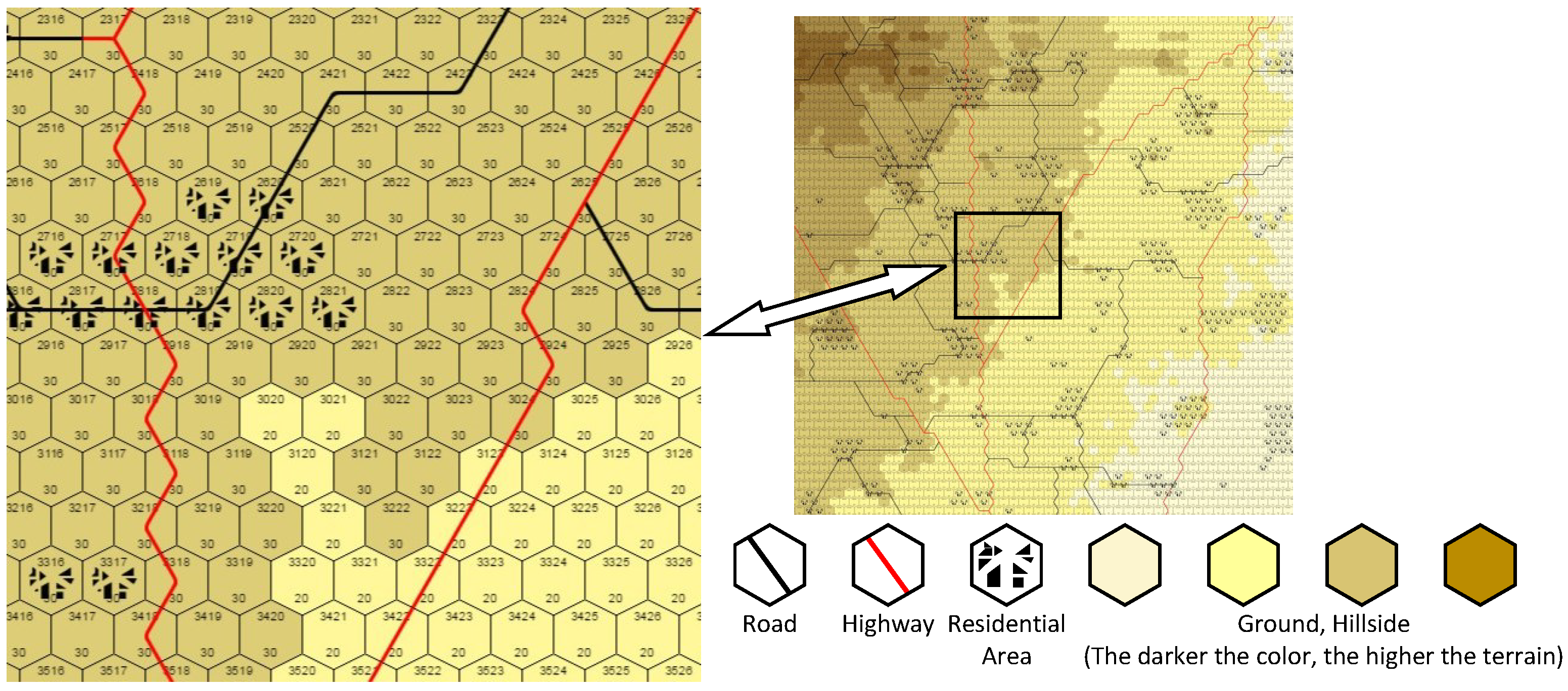
2.1. Tactical Wargame Platform

The armored assault group wargame system (AAGWS) (http://www.hexwar.cn/, accessed on 1 February 2025) is a tactical-level wargame simulation platform designed to meet the specific requirements of wargaming. It enables players to simulate realistic battlefield environments and explore the impact of their strategic decisions. Figure 1 illustrates a segment of the wargame map, divided into hexagonal grids, with each hexagon representing the smallest unit on the map. Each grid cell displays a numerical identifier at the top and a terrain type at the bottom, facilitating location identification and terrain analysis.

In this example, the map primarily shows urban residential areas, where opposing forces engage in offensive and defensive maneuvers to capture strategic points. The scoring system of this game is based on the number of points occupied and the effectiveness of each side attack. In the computerized wargame, players control multiple units (pieces), with each unit capable of performing various actions, such as moving or attacking, within a single turn. The objective of both sides is to secure key points through coordinated offensive and defensive strategies, with the outcome of the game determined by the number of occupied points and the results of offensive actions.

2.2. Dataset Description

In this work, we use the dataset processed by Liu et al. [19] as our baseline. This dataset contains data from 670 confrontation matches in AAGWS and consists of seven files that record comprehensive game information. Each game is documented in detail, including the initial state of each piece at the beginning (covering basic attributes such as position and type) and the state of each piece at the end of the game (indicating whether it is alive or in another state). Additionally, the dataset records the final status of occupied points, specifying which side controls each point. It also includes action records for each step taken by the pieces throughout the game, detailing movement paths, attack behaviors, and other operations. After parsing the dataset, the extracted features in AAGWS are categorized into attribute vectors and spatial tensors. The attribute vectors describe the attributes and action stages of the pieces, while the spatial tensors represent the situational data of the wargame. To distinguish between tensors and vectors, we define tensors in this context as arrays with dimensions greater than or equal to two. A detailed composition of these features is shown in

Table 1. Composition of data features.

Features	Sub-Features	Size	Description
Attribute vectors	Stage	20 bits	Stage of the wargame.
	Occupation points	4 bits	Status of occupation points.
	Our piece attributes	23 bits	138 bits total for 6 pieces.
	Enemy piece attributes	23 bits	138 bits total for 6 pieces.
	Result	1 bit	Labeled data for model training.
Spatial tensors	Player color	$1\times 66\times 51$	Red (0) or blue (1).
	Our pieces location	$6\times 66\times 51$	Locations of 6 pieces.
	Observed enemy locations	$6\times 66\times 51$	Locations of 6 enemy pieces.
	Enemy vehicle vision	$1\times 66\times 51$	Vision range of enemy vehicles.
	Enemy soldier vision	$1\times 66\times 51$	Vision range of enemy soldiers.
	Map tensor	$4\times 66\times 51$	Elevation of the map.
	Previous stage enemy locations	$6\times 66\times 51$	Labeled data for model training.

.

The attribute vectors are one-hot encoded and consist of a total of 301 bits. Most of the spatial tensors also use one-hot encoding, except for the elevation of the map, which is normalized to values between 0 and 1. The spatial tensor has a shape of $25\times 66\times 51$ in total. Due to only incomplete information being available for each side, the data features for the two opposing sides differ. After extracting the wargame features, we divided the dataset into training and test sets in a ratio of 8 to 2, ensuring that the ratio of winners to losers remained balanced at $1:1$ in both sets (the data includes perspectives from both the red and blue sides).

3. Methodology

In this section, we provide a detailed overview of the proposed enhanced location prediction model. Each module within the framework is illustrated to clarify its functionality within the overall architecture.

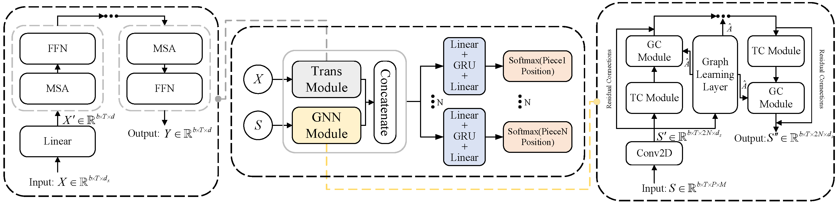
3.1. Framework

Given the crucial role of transformers in handling sequence data and the effectiveness of GNNs in processing spatial data, we now present the location prediction model for wargaming that leverages transformers and GNNs as core modules. Figure 2 illustrates the architecture of the proposed ELP-Net for wargaming. In this framework, the input attribute vector is denoted as $X:=\{X_1,\cdots ,X_T\}\in {\mathbb{R}}^{b\times T\times d_x}$, where T represents the length of the sequence, b is the batch size, and $d_x$ denotes the dimension of the input feature. The spatial tensor is represented as $S:=\{S_1,\cdots ,S_T\}\in {\mathbb{R}}^{b\times T\times P\times M}$, where $P=25$ is the size of the spatial tensor, and $M=66\times 51=3366$ corresponds to the total number of hexagonal grids on the map. The transformer module consists of linear layers, multi-head self-attention (MSA) mechanisms, and position-wise feed-forward (FFN) networks. The GNN module is structured with a Conv2D, a graph learning layer, temporal convolution (TC) modules, and graph convolution (GC) modules. After concatenating the transmissions of the spatial and attribute features, the network is divided into N blocks, each with the same architecture. To preserve temporal feature information, we utilize a gated recurrent unit (GRU), a variant of recurrent neural networks that is designed to manage information flow through update and reset gates. Finally, a fully connected layer of size M, followed by a softmax layer, is used to generate the output tensor for each piece.

In the following sections, we provide a detailed breakdown of each module to offer a comprehensive understanding of the proposed model. For reproducibility, a more detailed experimental setup is presented in Appendix A.

3.2. Transformer Module

In our model, the transformer module processes the attribute vector X. The architecture consists of a sequence of transformer layers, each composed of a multi-head self-attention (MSA) mechanism and a feed-forward network (FFN). In the following, we use a single-head self-attention module for illustration.

Firstly, a linear transformation is applied to the input attribute vector X, producing $X^{\prime }\in {\mathbb{R}}^{b\times T\times d}$ with a hidden dimension d. Then, the self-attention module projects $X^{\prime }$ into three subspaces, namely Q (queries), K (keys), and V (values):

$$Q=X^{\prime }{W}_Q,K=X^{\prime }{W}_K,V=X^{\prime }{W}_V,$$

(1)

where $W_Q\in {\mathbb{R}}^{d\times d_w}$, $W_K\in {\mathbb{R}}^{d\times d_w}$, and $W_V\in {\mathbb{R}}^{d\times d_v}$ are learnable projection matrices. These matrices map $X^{\prime }$ into the query matrix (Q), key matrix (K), and value matrix (V). The dimension $d_w$ corresponds to the feature size of Q and K, while $d_v$ represents the feature size of V. These dimensions are used to scale the attention mechanism.

Next, the attention matrix is computed to capture the pairwise similarity between the input features in the sequence:

$$Attn\left(X^{\prime }\right)=\mathrm{softmax}({\displaystyle \frac{Q{K}^T}{\sqrt{d_w}}})V,$$

(2)

where $Attn\left(X^{\prime }\right)$ measures the similarity between each pair of projected feature vectors (queries and keys) by calculating their dot product. The resulting scores are scaled by $\sqrt{d_w}$ to ensure numerical stability, particularly for large dimensions. The softmax function is applied row-wise to normalize these attention scores, enabling the model to assign appropriate weights to different parts of the sequence.

The MSA mechanism enhances the model ability to capture and express information by dividing the input into multiple self-attention heads. Each head calculates self-attention in parallel, and the outputs of all heads are then concatenated to increase the representational capacity of the model. The computation of MSA is as follows:

$$MSA\left(X^{\prime }\right)={\left|\right|}_{h-1}^H\left(Att{n}^{\left(h\right)}\left(X^{\prime }\right)\right),$$

(3)

where $\left|\right|$ denotes a concatenation operation and H is the number of attention heads. Similarly, each head h computes its own attention as

$$Att{n}^{\left(h\right)}\left(X^{\prime }\right)=\mathrm{softmax}(Q^{\left(h\right)}{(K^{\left(h\right)})}^T/\phantom{Q^{\left(h\right)}{\left(K^{\left(h\right)}\right)}^T\sqrt{d_w}}\sqrt{d_w})V^{\left(h\right)}.$$

(4)

The FFN consists of two linear layers with a GELU [35] non-linearity, which is implemented similarly to the approach by Chen et al. [36]. Finally, the layer-wise computation in the transformer module is defined as follows:

$$Y^{\prime \left(l\right)}=MSA\left(LN\left(Y^{(l-1)}\right)\right)+Y^{(l-1)},$$

(5)

$$Y^{\left(l\right)}=FFN\left(LN\left(Y^{\prime \left(l\right)}\right)\right)+Y^{\prime \left(l\right)},$$

(6)

where $Y^{\left(0\right)}=X^{\prime }$, $l\in \{1,\dots ,L\}$ denotes the l-th layer of the transformer module and $LN(·)$ represents the normalization operation.

3.3. Spatial–Temporal Graph Neural Network

We employed a spatial–temporal graph neural network module on the wargame data to improve feature representation learning and to effectively capture both spatial and temporal dependencies.

3.3.1. Graph Learning Layer

In wargaming, the positional data of the pieces exhibit significant sparsity. At the same time, the movement of these pieces is not arbitrary, it is governed by various factors such as occupied points, opposing units, and terrain types. To effectively model this complex behavior, we introduce a graph learning layer that constructs a graph data structure, one that is capable of adaptively extracting a sparse graph adjacency matrix. This matrix reflects the inherent characteristics and potential relationships within the data.

While distance measures such as dot product and Euclidean distance are commonly used to quantify the similarity between node pairs, these measures are typically symmetric or bidirectional. However, in multivariate wargame piece prediction, the relationships among pieces are often unidirectional, as the state change of one piece can influence the states of others in a directed manner. To capture these unidirectional relationships, we use a graph learning layer, which is defined by the following equations:

$$A_t=\mathrm{softmax}(tanh\left(S_t^{\prime }{W}_1\right)tanh\left(W_2^T{S}_t^{\prime T}\right)),\forall t\in \{1,\cdots ,T\},$$

(7)

$$A_t[i,-idx]=0,idx=argtopk\left(A_t[i,:]\right),\forall i\in \{1,\cdots ,N\},$$

(8)

where $S_t^{\prime }$ represents the spatial feature embedding of the pieces at time t, and $W_1$ and $W_2$ are learnable parameter matrices that are optimized during training. Originally proposed by [37], Equation (7) generates an asymmetric graph adjacency matrix $A_t$. Equation (8) then selects the top-k nodes as neighbors for each node, and it is implemented using the $argtopk(·)$ function.

This graph learning layer is designed to capture the dynamic spatial dependency relationships of the pieces. It adjusts the connections between nodes in the graph structure based on the input features of each situational graph. This dynamic adjustment of node relationships over time enables the model to capture temporal dependencies and spatial correlations effectively.

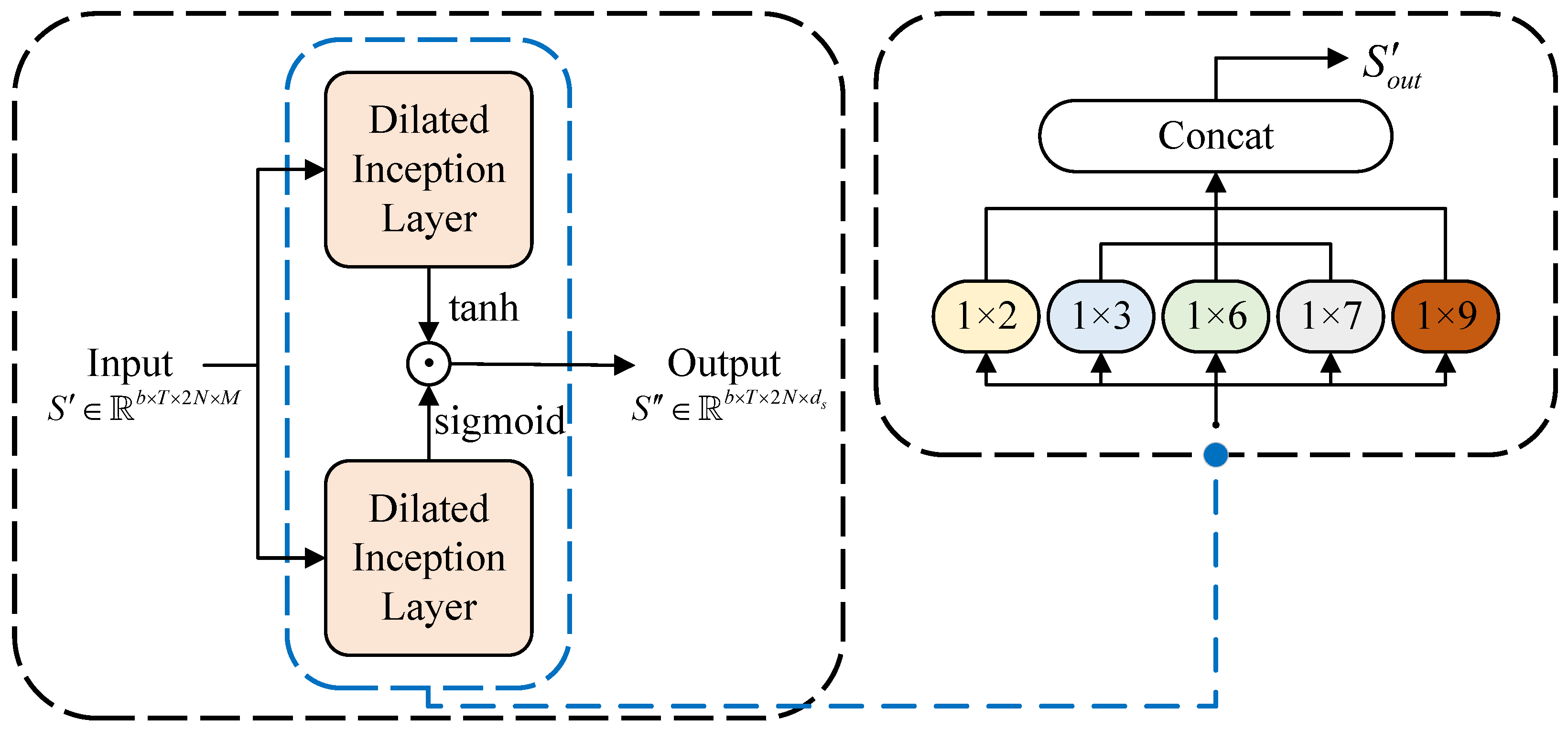
3.3.2. Temporal Convolution Module

Situational maps typically contain not only the spatial relationships among various nodes, but also the dynamic changes that occur over time, exhibiting strong local correlations between adjacent time steps. To leverage these temporal dependencies, time convolution is employed to effectively capture the associated features of the situational data across successive time steps.

The temporal convolution module consists of two dilated inception layers [38], each containing a series of standardized one-dimensional convolution filters. One layer employs a hyperbolic tangent (tanh) activation function, serving as a filter to extract high-level temporal features. The other layer utilizes a sigmoid activation function, acting as a gating mechanism to regulate the flow of information from the filter to subsequent modules. This dual-layer structure enables the module to balance feature extraction and information flow effectively. The architecture of the temporal convolution module is illustrated in Figure 3.

To address the periodicity in the time-series data of situational graphs, we combine filters of varying sizes with dilated convolutions. The dilated inception layer incorporates five filter sizes: $1\times 2$, $1\times 3$, $1\times 6$, $1\times 7$, and $1\times 9$. To handle long sequences efficiently, dilated convolution is employed to expand the receptive field size, enabling the network to capture long-range dependencies while maintaining computational efficiency.

The input to the temporal convolution module is $S^{\prime }\in {\mathbb{R}}^{b\times T\times 2N\times d_s}$, where $2N$ represents the total number of pieces from both the red and blue sides, and $d_s$ is the hidden dimension. The dilated convolution is defined as follows:

$$S^{\prime }\otimes f_{1\times c}={\sum }_{i=0}^{c-1}{f}_{1\times c}\left(i\right)S^{\prime }(t-a\times i),$$

(9)

where ⊗ represents the convolution operation, $f_{1\times c}\left(i\right)$ denotes the i-th value of the filter with size c, a is the dilation factor, and $t\in \{1,\cdots ,T\}$ represents the current time step in the sequence.

Then, the outputs of the five filters are truncated to the same length according to the largest filter size, and they are they concatenated across the channel dimension:

$$S_{out}^{\prime }=concat(S^{\prime }\otimes f_{1\times 2},S^{\prime }\otimes f_{1\times 3},S^{\prime }\otimes f_{1\times 6},S^{\prime }\otimes f_{1\times 7},S^{\prime }\otimes f_{1\times 9}),$$

(10)

where $concat$ represents concatenation, which aggregates the features extracted by filters of different sizes, allowing the model to capture temporal patterns with varying scales and periodicities.

Finally, the outputs from the two dilated inception layers are individually processed by two activation functions. The resulting outputs are then combined using a Hadamard product to produce the final output, $S^{″}$.

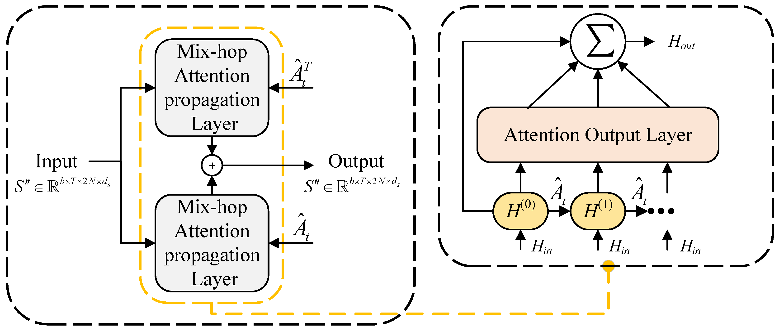
3.3.3. Graph Convolution Module

In wargaming, the movement trajectories of pieces are affected by other pieces. The purpose of introducing the graph convolution module is to fuse the information of a node with that of its adjacent nodes in order to handle the spatial dependency relationships in the graph. We propose a new mix-hop attention propagation layer to adaptively learn the importance of different graph convolution layers, thereby further enhancing the model performance. Figure 4 shows the architectures of the graph convolution module and the proposed mix-hop attention propagation layer.

The new mix-hop attention propagation layer in this module includes two steps: information propagation and information selection. The information propagation step is formulated as follows:

$$H^{\left(l\right)}=\alpha H_{in}+(1-\alpha ){\widehat{A}}_t{H}^{(l-1)},$$

(11)

where $H_{in}$ represents the input hidden states produced by the previous layer, with $H^{\left(0\right)}=S^{″}$ the output from the temporal convolution module; $\alpha$ is a hyperparameter that controls the ratio of the original root node states to be retained; and $l\in \{1,\cdots ,L\}$ denotes the propagation depth. For the graph convolution, we use the asymmetrically normalized adjacency matrix ${\widehat{A}}_t$, with ${\widehat{A}}_t={\widehat{D}}^{-1}(A_t+I)$, and $\widehat{D}$ is the degree matrix. The asymmetrically normalized adjacency matrix enables the model to effectively utilize the direction information of edges in a directed graph.

The information propagation step recursively disseminates node information according to the given graph structure. However, as the number of layers in the graph convolution network increases, the model often encounter the issue of over-smoothing. To address this problem, we introduce self-attention mechanisms [25] in the information selection step to retain the important information generated at each convolution layer. The information selection step is defined as follows:

$$H_{out}={\sum }_{l=0}^L(Att{n}^{\left(l\right)}\left(H^{\left(l\right)}\right)+H^{\left(l\right)}),$$

(12)

where $H_{out}$ represents the output hidden states of the current layer l.

The graph convolution module consists of two mix-hop attention propagation layers, which process the inflow and outflow information through each node. The final output of the graph convolution module is obtained by summing the outputs of the two mix-hop attention propagation layers.

3.4. Optimization

The optimization process utilizes the cross-entropy loss function, which is defined as follows:

$$\mathcal{L}(X,S)={\displaystyle \frac{1}{T}}{\displaystyle \frac{1}{M}}{\displaystyle \sum _{t=1}^T}{\displaystyle \sum _{i=1}^N}{\displaystyle \sum _{j=1}^M}-P\left({\phi }_j^i\right|X_t,S_t)log{\tilde{P}}_{\theta }\left({\phi }_j^i\right|X_t,S_t),$$

(13)

where X represents the set of attribute vectors over $T=10$ time steps, and S denotes the set of spatial tensors. The total number of opponent pieces is $N=6$, and the total amount of hexagonal grids is $M=3366$. The term $P\left({\phi }_j^i\right|X_t,S_t)$ is the true probability of the i-th piece being located on the j-th grid given the input features X and S. Conversely, ${\tilde{P}}_{\theta }\left({\phi }_j^i\right|X_t,S_t)$ denotes the predicted probability of the i-th piece being on the j-th grid, and it is generated by the proposed ELP-Net with the set of model parameters $\theta$. The complete algorithm is presented in Algorithm 1. Further complexity analysis of our model is provided in Appendix C.

Algorithm 1 The predictive algorithm of ELP-Net

Input: batch of sampled data ($X\in {\mathbb{R}}^{b\times T\times d_x},S\in {\mathbb{R}}^{b\times T\times P\times M}$); initialized graph learning layer $f_{A_t}(·)$; initialized temporal convolution module $f_T(·)$; initialized graph convolution module $f_G(·)$; parameter set $\theta$; learning rate $\gamma$.  1: repeat  2:    process piece attribute features using the transformer: $Y=\mathrm{Trans}\left(X\right)$.  3:    perform spatial feature transformation: $S^{\prime }=\mathrm{Conv}2\mathrm{D}\left(S\right)$.  4:    construct the adjacency matrix of pieces: $A_t=f_A(S^{\prime };S^{\prime T})$.  5:    process spatial features with temporal convolution: $S^{″}=f_T\left(S^{\prime }\right)$.  6:    aggregate spatial information using graph convolution: $S^{″}=f_G(S^{″};A_t;A_t^T)$.  7:    integrate temporal and spatial features for all pieces:  8:    for n in $1:N$ do  9:       $Z_{list}=Z_{list}.append\left(\mathrm{GRU}\left(concat(Y;S^{″})\right)\right)$. 10:   end for 11:   stack outputs across all pieces: $Z=stack\left(Z_{list}\right)$. 12:   compute the loss: $\mathcal{L}=(\tilde{P}(Z;\theta );P)$. 13:   update model parameters $\theta$ according to gradients and learning rate $\gamma$. 14: until convergence

4. Experimental Results

In this section, we present the evaluation of ELP-Net on the location prediction task using the wargame dataset. The train and test results are presented in Section 4.3 and Section 4.4, which are followed by an analysis of the impact of network depth on the performance of our model in Section 4.5. Finally, the contributions of different modules to the overall model framework are discussed in Section 4.6.

4.1. Experimental Setting

To evaluate the prediction accuracy of ELP-Net, we use a performance metric that measures the probability of the ground truth labels falling within the top 1, 3, 5, 10, 15, and 50 hexagonal grids with the highest predicted probabilities. This provides a comprehensive assessment of the model accuracy across varying levels of prediction confidence. For model training, the ADAM optimizer [39] is employed to ensure efficient and stable convergence. The main hyperparameters used in the training process are summarized in

Table 2. Parameter settings.

Module	Parameters	Value
Transformer	Number of heads H	8
	Dropout	0.1
GNN	Depth L of mix-hop	3
	Retain ratio $\alpha$ of mix-hop	0.05
Others	Learning rate $\gamma$	0.001
	Learning decay rate	0.7
	Time steps T	10
	Weight decay	0.0001
	Mini-batch size b	32
	Epochs	15

. Further details on the implementation are provided in Appendix B.

4.2. Baseline Methods for Comparison

To validate the effectiveness and practicality of ELP-Net, we conducted a comparative experiment between the following methods. All models were trained using a dataset split with a ratio of 8:2 for the training and test sets:

• CNN-GRU: The model proposed by Liu et al. [19], combining convolutional neural networks (CNNs) and gated recurrent units (GRUs).
• CNN-MSA-GRU: An enhanced version of the CNN-GRU model with the addition of a multi-head self-attention (MSA) module.
• ELP-Net: Our proposed model, integrating a graph learning layer, graph convolution, temporal convolution modules, and transformer architecture for improved feature representation and prediction accuracy.

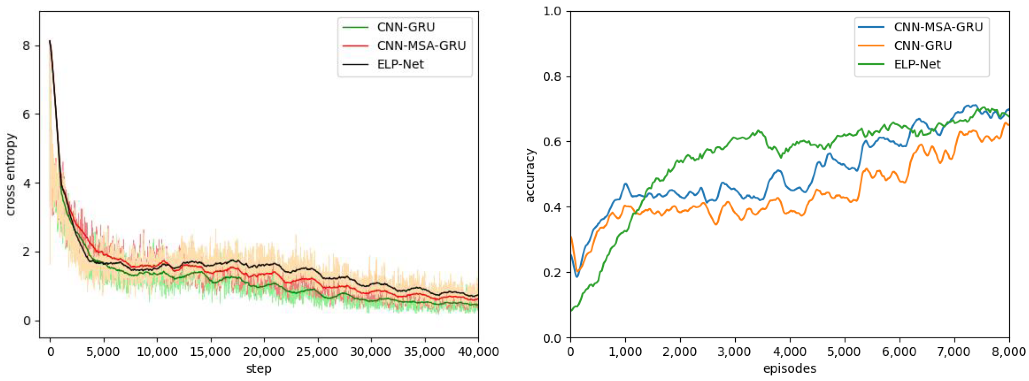
4.3. Train Results

Based on the wargaming dataset, we trained three network models: CNN-GRU, CNN-MSA-GRU, and ELP-Net. Figure 5 illustrates the comparison of their training results, including the loss and accuracy curves recorded after each mini-batch. In the left panel, the loss values of all models are shown per training step, while the right panel presents accuracy values, which are calculated every 10 time steps as one episode. From the figure, it is evident that the loss curves for all models converge over time, demonstrating stable training. The ELP-Net model exhibits a slightly higher loss during training, likely due to the integration of the GNN and transformer modules. These components significantly improve model capacity but at the cost of increased complexity. Consequently, ELP-Net achieves the highest accuracy among the three models, benefiting from its ability to capture both spatial and temporal dependencies effectively.

During the training process, validation on the test dataset revealed some degree of overfitting in all models. To ensure better generalization and optimal test results, we selected the model parameters corresponding to the highest top 1 average accuracy on the validation set as the final parameters for testing.

4.4. Test Results

This section presents the test results for the proposed model ELP-Net, where its performance against other models and across different types of wargame pieces is compared.

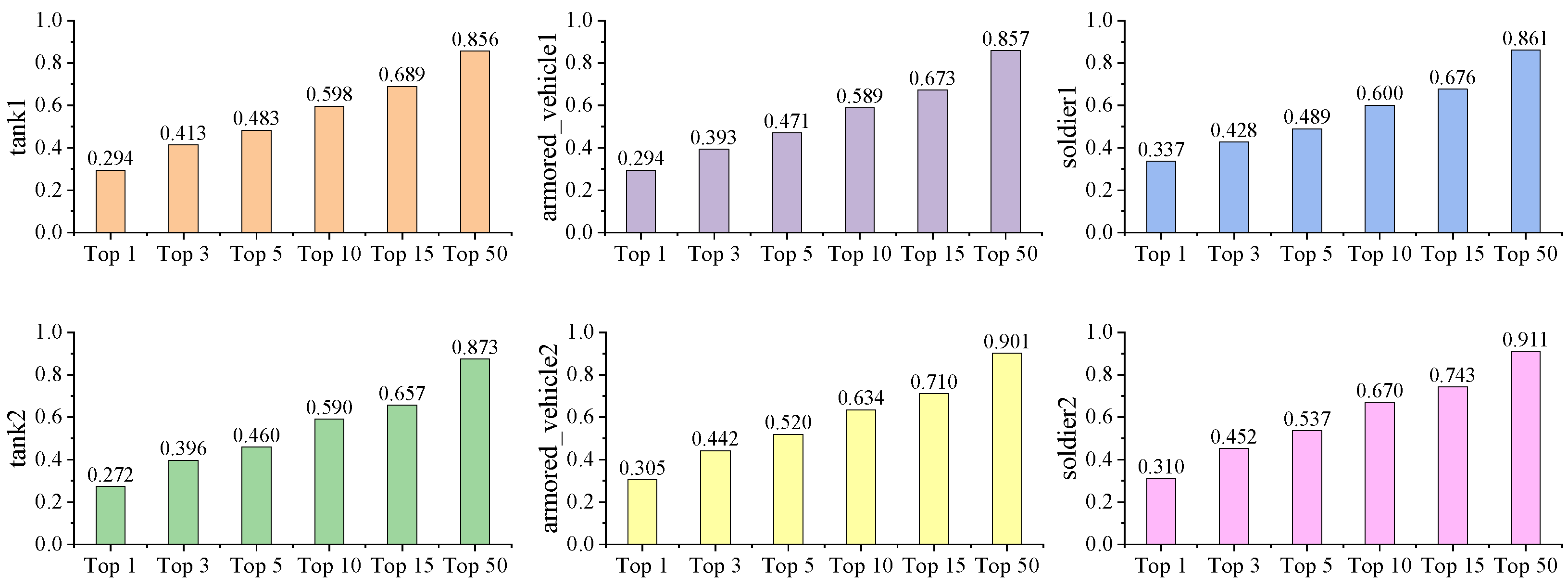
4.4.1. Top-x Accuracy Between Different Pieces

Firstly, we tested the ELP-Net under optimal verification parameters and selected the highest accuracy as the baseline result. Figure 6 presents the top 1, top 3, top 5, top 10, top 15, and top 50 prediction accuracy for all pieces using ELP-Net. Overall, the results reveal that the soldier2 piece consistently achieves the highest accuracy across all top-x levels, followed by the armored vehicle2 pieces, with the tank1 pieces exhibiting the lowest accuracy. From an operational perspective, this pattern aligns with the actual complexity of the battlefield. Soldier pieces are more dynamic and likely engage in smaller areas, making them easier to predict accurately. In contrast, tank pieces operate over larger areas with more significant movement restrictions, resulting in greater prediction uncertainty. Similarly, armored vehicle pieces exhibit intermediate accuracy, reflecting their moderate maneuverability and constrained operational zones.

For decision makers, it is not essential to point to the exact hexagonal grid where the opponent pieces are located. Instead, it is more critical to identify the approximate range of hexagonal grids in which the opponent pieces are likely to be. Consequently, top 5, top 10, and top 15 prediction results are practically usable metrics as they strike a balance between accuracy and operational applicability in complex wargame scenarios.

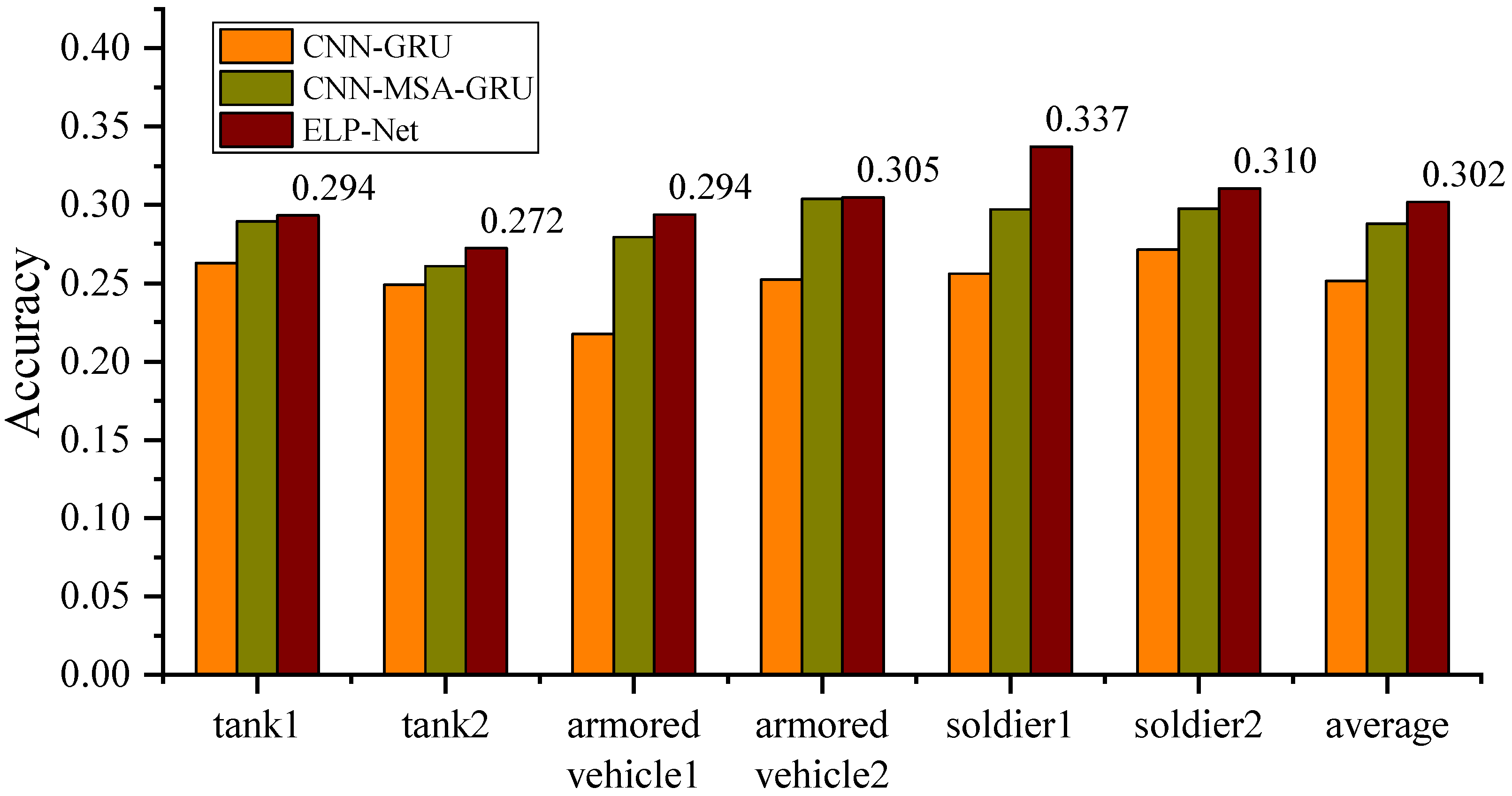
4.4.2. Top 1 Accuracy Among Different Models

In addition, we compared the testing accuracies of the three models on top 1 accuracy, as well as the average accuracy across all pieces for top 1 predictions. Figure 7 illustrates the testing accuracy for individual pieces and the average testing accuracy across all pieces. From the figure, it is evident that our proposed model ELP-Net achieves the highest prediction accuracy for all pieces and also outperforms others in terms of overall average accuracy. When comparing the two baseline models, CNN-GRU and CNN-MSA-GRU, the addition of the GNN module in ELP-Net leads to significantly improved performance. This highlights the critical role of the GNN in processing situational map data by effectively capturing spatial relationships. Similarly, the transformer module, particularly with the addition of the MSA mechanism, demonstrates its decisive role in handling time-series data, outperforming the CNN-GRU model. In summary, the combination of the transformer module and the GNN module results in superior performance, making ELP-Net the most effective among the evaluated methods.

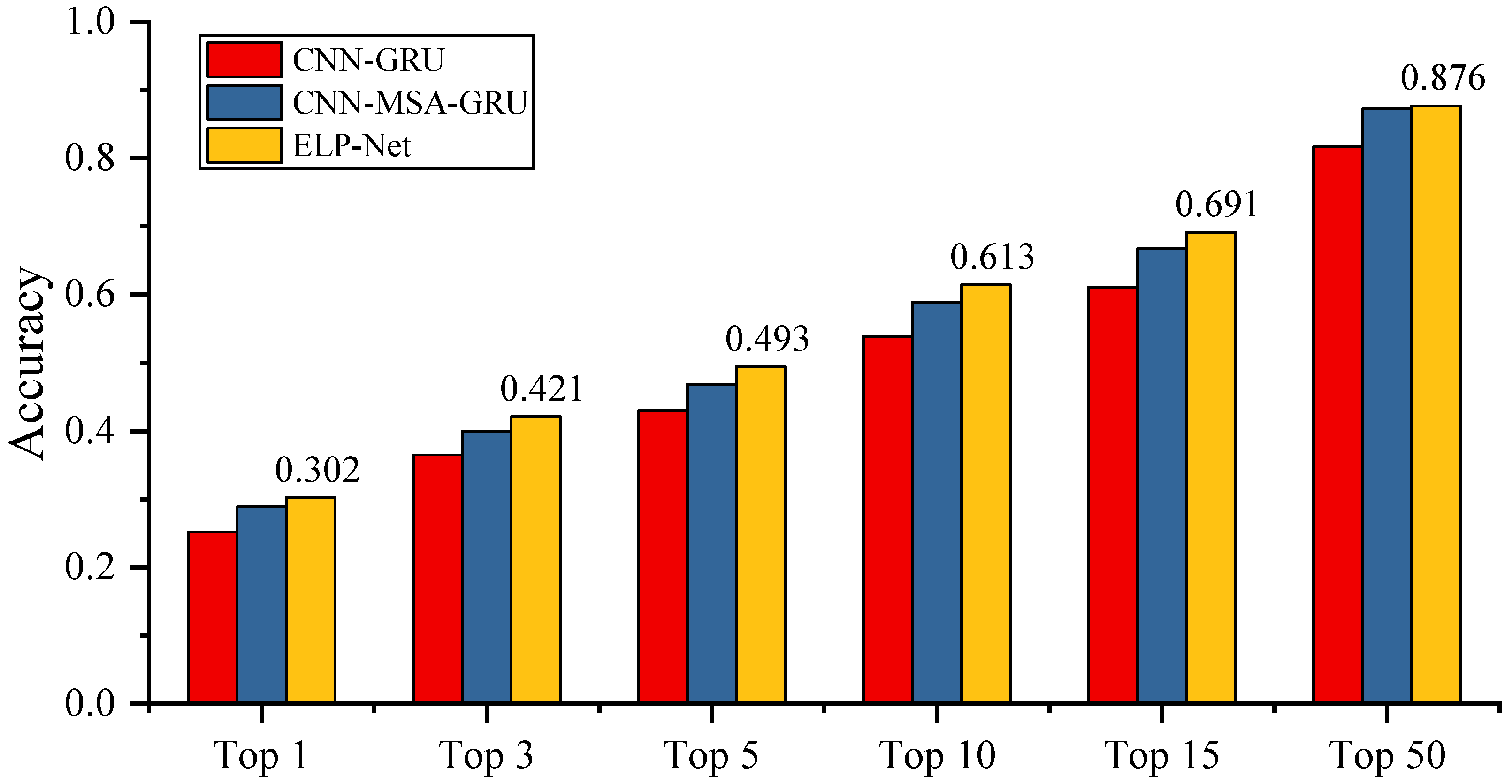
4.4.3. Averaged Top-x Accuracy Comparison Between Competitors

Moreover, Figure 8 compares the averaged test accuracy of the three models across top-x predictions. The results indicate that introducing the MSA mechanism in the CNN-MSA-GRU model yields noticeable performance gains compared to the CNN-GRU model. At each top-x level, the accuracy of CNN-MSA-GRU surpasses that of CNN-GRU, highlighting the MSA ability to capture richer temporal dependencies and improve feature extraction from sequential data. Additionally, the ELP-Net model consistently achieves the highest test accuracy at every top-x level, demonstrating its effectiveness in improving prediction accuracy and outperforming the baseline models. The consistent improvements of ELP-Net can be attributed to its integration of GNNs for spatial dependency modeling and transformer module for capturing temporal relationships. By leveraging these advanced components, ELP-Net effectively combines spatial and temporal information, enabling more robust and accurate location predictions in complex wargaming scenarios.

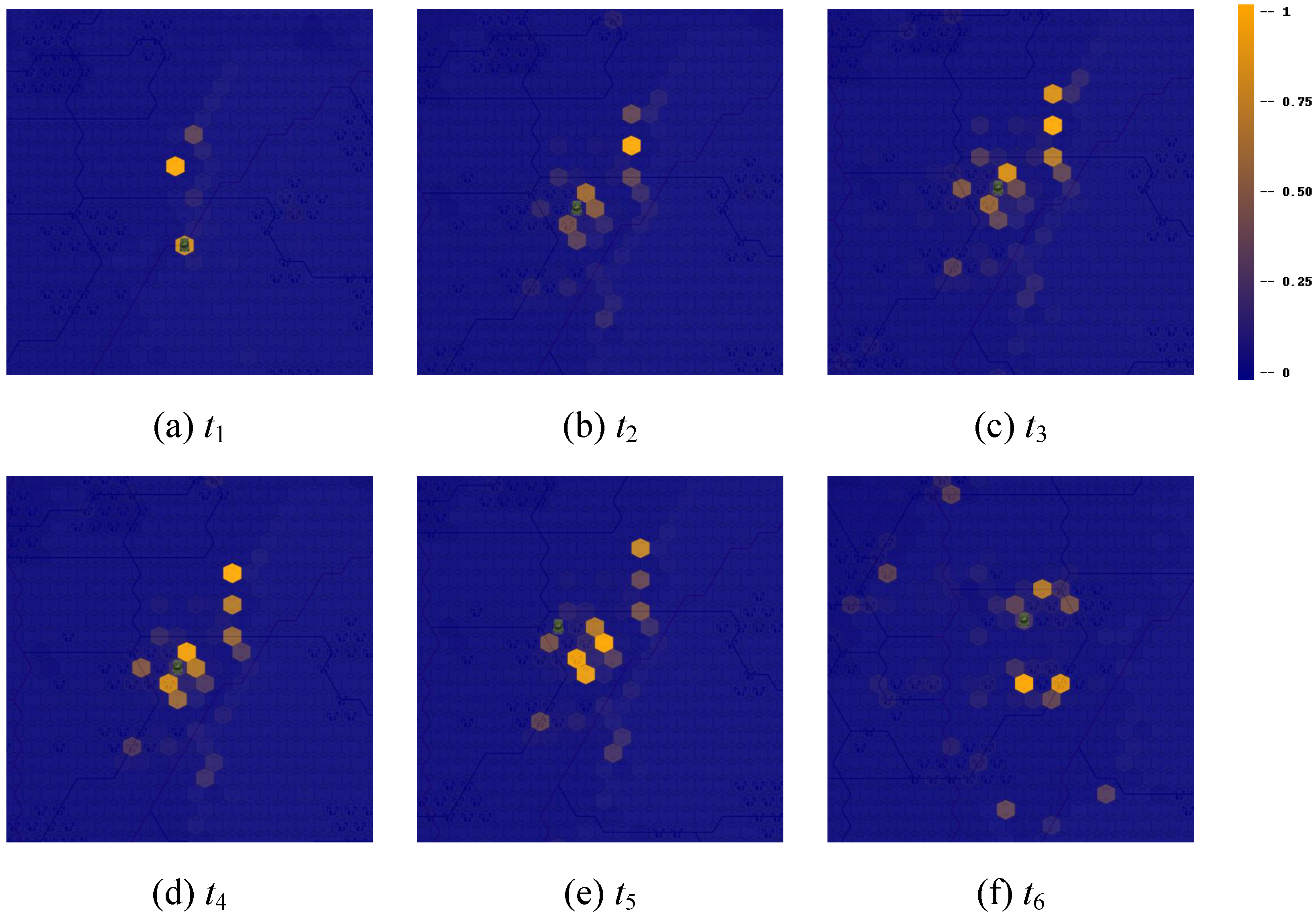
4.4.4. Enemy Location Prediction Heatmap

In Figure 9, the location prediction heatmap generated by the ELP-Net model and the actual locations of the tank2 piece in different time periods are presented. The predicted probabilities of enemy locations are normalized to the interval $[0,1]$ to represent their likelihoods. The actual locations of the piece, represented as a green tank on the map, correspond to the true positions in the wargame. As time goes by, the activity range of the tank gradually expands. This is reflected in the heatmap by the increasing number of lighter-colored hexagonal grids, indicating a wider distribution of predicted probabilities. At time $t_1$, the prediction accuracy was the highest as the tank was more stationary and its location was easier to predict. However, as the tank moved further and its operational range broadened, the distribution of predicted probabilities became more dispersed, leading to a decrease in prediction accuracy.

Despite this, it is worth noting that, while the actual locations of the tank are not always on the hexagonal grid with the highest predicted probability, they are typically in close proximity to it. This proximity allows decision makers to effectively narrow down the potential locations of enemy units. As a result, this reinforces the practical value of using top-x accuracy, such as top 5 or top 10, over top 1 accuracy in real-world applications as it provides actionable information for decision making in dynamic and uncertain environments.

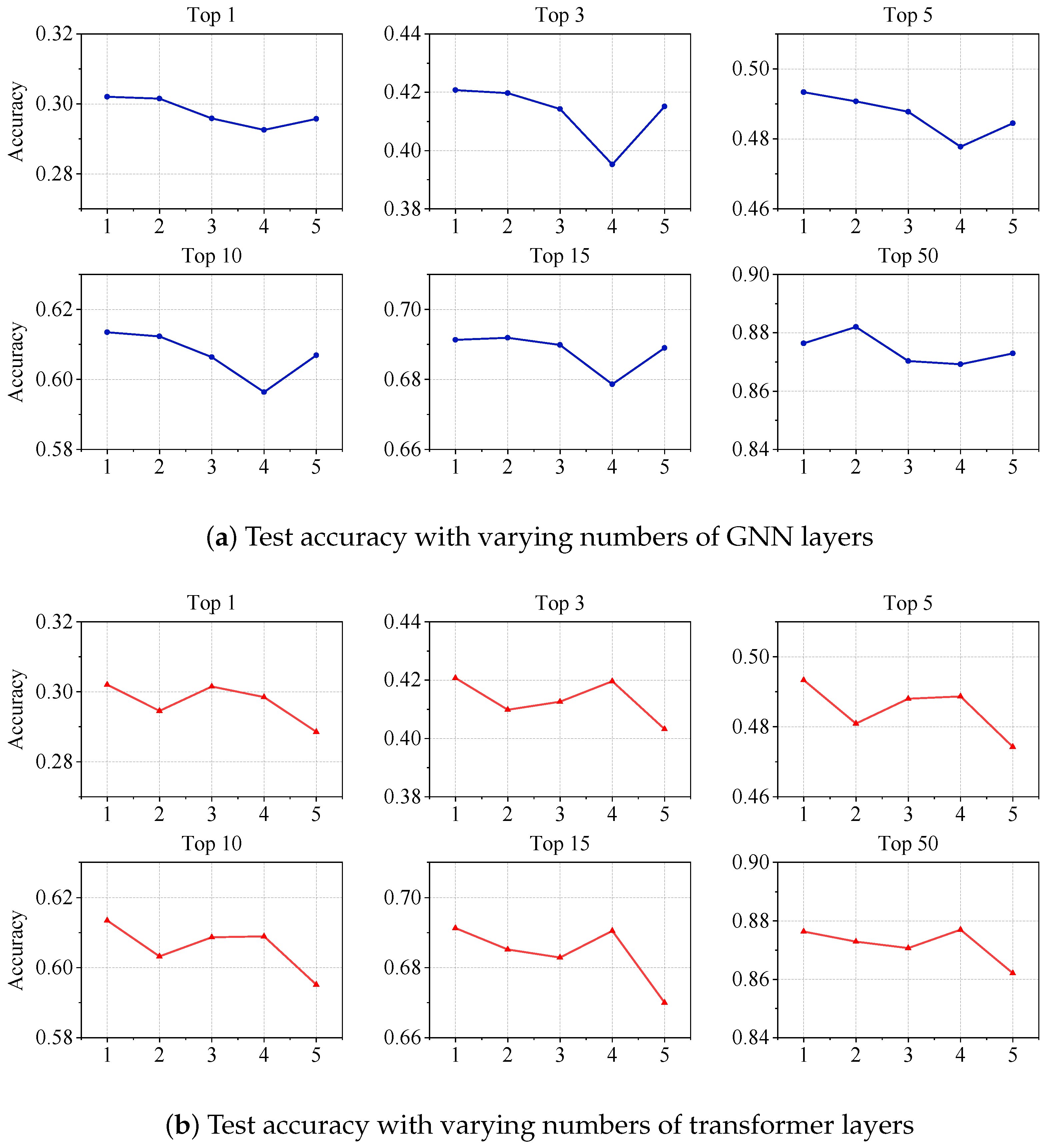
4.5. Network Depth Influence

To further evaluate the performance of ELP-Net, we investigated the impact of two critical parameters: the number of layers in the GNN module and the number of layers in the transformer module. Specifically, Figure 10 presents the test accuracy results with varying numbers of GNN and transformer layers.

For the GNN module, the number of transformer layers was fixed at 1, and the number of GNN layers was varied from 1 to 5. The results (Figure 10a) show that using a single GNN layer achieves the best performance across most top-x levels. However, for broader prediction ranges like top 15 and top 50, a depth of two layers yields slightly better accuracy. This suggests that, for more localized predictions, a single layer is sufficient to capture the spatial relationships effectively, while additional layers provide a benefit when broader contextual information is required. For the transformer module, we fixed the number of GNN layers at 1 and varied the number of transformer layers from 1 to 5. The general trend, as presented in Figure 10b, showed a decrease in accuracy as the number of layers increased. A single transformer layer achieved optimal performance for most top-x levels, while for top 3, top 15, and top 50, a depth of four layers delivered comparable results. This could be attributed to the model ability to capture longer temporal dependencies at these specific prediction levels when additional layers are used. However, beyond this, the increased complexity likely leads to overfitting and diminished performance.

These findings suggest that both the transformer and GNN modules require careful tuning of their respective layer depths to avoid overfitting and to maximize performance. A smaller number of layers often provides a more optimal trade off between model complexity and generalization.

4.6. Ablation Study

In the previous study, we developed a composite model, ELP-Net, integrating both the spatial–temporal GNN module and the transformer module. To further assess the contributions of these components, the following analysis presents an ablation study on ELP-Net, examining the specific impacts of each module individually and in combination with the overall model performance. We define the variants of ELP-Net by removing different components as follows.

• Base model: a version of the model without transformer and GNN modules.
• +Transformer: the base model with the addition of transformer module.
• +GNN: the base model with the GNN module added.
• Full model: the complete ELP-Net, with both the transformer and GNN modules.

As shown in

Table 3. Impact of different modules on the top-x prediction accuracy and average performance.

Model Variant	Top 1	Top 3	Top 5	Top 10	Top 15	Top 50	Average
Base model	0.251	0.365	0.430	0.539	0.610	0.817	0.502
+Transformer	0.288	0.399	0.468	0.588	0.667	0.872	0.547
+GNN	0.291	0.394	0.462	0.579	0.677	0.867	0.545
Full model	0.302	0.421	0.493	0.613	0.691	0.876	0.566

, adding the transformer module alone results in an average performance improvement of $4.5\%$. This indicates the ability of the transformer to extract effective feature patterns from the time-series data of piece attribute features. By capturing the temporal evolution of the pieces’ attributes, the transformer helps the model better understand the dynamics of the pieces over time, leading to more accurate predictions of their future positions.

Introducing the GNN module alone resulted in an average performance improvement of $4.3\%$. This means that the GNN successfully captured the key spatial information contained in the spatial situational data, such as the relative distances between pieces, mutual attack ranges, and cluster structures. These spatial factors significantly influence the changes in piece positions. By iteratively propagating and aggregating information, the GNN allows each piece to incorporate features from its surrounding environment. This enriched spatial relationship information enables the model to make more informed predictions about piece positions.

When both the GNN and transformer modules are added simultaneously, the model achieves an average performance improvement of $6.4\%$. This improvement surpasses the gains that are achieved using either module alone, highlighting the synergistic effect between the two modules. The transformer focuses on the temporal patterns of the piece attribute features over time, while the GNN concentrates on the position relationships and their dynamic evolutions in the spatial situational data. This combination allows for a more comprehensive understanding of the factors affecting position changes, enabling the model to make more accurate and reliable predictions.

5. Discussion

The results of this study highlight the superior performance of the proposed ELP-Net in the task of location prediction for wargaming. ELP-Net consistently outperformed the baseline models in both top 1 and top x accuracy. These results demonstrate the robustness and adaptability of ELP-Net in complex wargaming scenarios, providing a significant advancement in this field. Despite these strengths, there are still several areas for further improvement. Addressing these limitations will not only refine the performance of ELP-Net, but also extend its applicability to broader domains.

• Generalization of the graph learning layer: The current approach of constructing a graph adjacency matrix for each time step of the situational graph using the graph learning layer shows limitations in generalizability. Future research could explore the impact of diverse graph topologies on model performance and develop adaptive graph construction methods that automatically select the optimal graph structure based on the data. This enhancement would improve the model applicability across diverse datasets.
• Optimization of the temporal convolution module: While employing multiple-sized dilated convolution filters aims to capture temporal patterns more comprehensively, it also increases model complexity. Future work could focus on refining the temporal convolution mechanism, potentially exploring alternative architectures or mechanisms that balance performance improvement with model simplicity.

By addressing these limitations, we aim to further refine ELP-Net, ensuring it remains a scalable, flexible, and interpretable solution for location prediction in tactical and strategic wargames.

6. Conclusions

This study presents ELP-Net, a novel location prediction model for wargaming that integrates graph learning and transformer-based temporal modeling to improve the accuracy of opponent location forecasting. By leveraging a spatial–temporal GNN module and a transformer-based sequence learning framework, ELP-Net effectively mitigates the challenges posed by data sparsity, high redundancy, and dynamic opponent strategies.

To promote further research and practical deployment, we have publicly released the source code of ELP-Net on GitHub (URL provided in Appendix B). Future research directions could include the following: expanding ELP-Net to real-world military and security applications, optimizing the model for real-time inference, and exploring reinforcement learning for adaptive decision making.

By addressing these challenges and expanding its scope, ELP-Net contributes to intelligent decision making in complex adversarial environments, bridging the gap between AI-driven strategic reasoning and real-world wargaming applications.

References

- Dunnigan, J.F. Wargames Handbook: How to Play and Design Commercial and Professional Wargames; IUniverse: Bloomington, IN, USA, 2000. [Google Scholar]
- Bolling, R.H. The Joint Theater Level Simulation in military operations other than war. In Proceedings of the 27th Conference on Winter Simulation, Arlington, VA, USA, 3–6 December 1995; pp. 1134–1138. [Google Scholar]
- Silver, D.; Huang, A.; Maddison, C.J.; Guez, A.; Sifre, L.; Van Den Driessche, G.; Schrittwieser, J.; Antonoglou, I.; Panneershelvam, V.; Lanctot, M.; et al. Mastering the game of Go with deep neural networks and tree search. Nature 2016, 529, 484–489. [Google Scholar] [CrossRef] [PubMed]
- Mnih, V.; Kavukcuoglu, K.; Silver, D.; Rusu, A.A.; Veness, J.; Bellemare, M.G.; Graves, A.; Riedmiller, M.; Fidjeland, A.K.; Ostrovski, G.; et al. Human-level control through deep reinforcement learning. Nature 2015, 518, 529–533. [Google Scholar] [CrossRef] [PubMed]
- Shao, K.; Zhu, Y.; Zhao, D. Starcraft micromanagement with reinforcement learning and curriculum transfer learning. IEEE Trans. Emerg. Top. Comput. Intell. 2018, 3, 73–84. [Google Scholar] [CrossRef]
- Vinyals, O.; Babuschkin, I.; Czarnecki, W.M.; Mathieu, M.; Dudzik, A.; Chung, J.; Choi, D.H.; Powell, R.; Ewalds, T.; Georgiev, P.; et al. Grandmaster level in StarCraft II using multi-agent reinforcement learning. Nature 2019, 575, 350–354. [Google Scholar] [CrossRef] [PubMed]
- Davis, P.K. Applying Artificial Intelligence Techniques to Strategic-Level Gaming and Simulation; Technical Reports; Rand Corporation: Santa Monica, CA, USA, 1988; Volume 2752. [Google Scholar]
- Bowling, M.; Fürnkranz, J.; Graepel, T.; Musick, R. Machine learning and games. Mach. Learn. 2006, 63, 211–215. [Google Scholar] [CrossRef]
- Langreck, J.; Wong, H.; Hernandez, A.; Upton, S.; McDonald, M.; Pollman, A.; Hatch, W. Modeling and simulation of future capabilities with an automated computer-aided wargame. J. Def. Model. Simul. 2021, 18, 407–416. [Google Scholar] [CrossRef]
- Hieb, M.; Hille, D.; Tecuci, G. Designing a Computer Opponent for War Games: Integrating Planning, Learning and Knowledge Acquisition in WARGLES. In Proceedings of the 1993 AAAI Fall Symposium on Games: Learning and Planning, Raleigh, NC, USA, 22–24 October 1993. [Google Scholar]
- Schwarz, J.O.; Ram, C.; Rohrbeck, R. Combining scenario planning and business wargaming to better anticipate future competitive dynamics. Futures 2019, 105, 133–142. [Google Scholar] [CrossRef]
- Moy, G.; Shekh, S. The application of AlphaZero to wargaming. In AI 2019: Advances in Artificial Intelligence, Proceedings of the 32nd Australasian Joint Conference, Adelaide, SA, Australia, 2–5 December 2019; Springer: Berlin/Heidelberg, Germany, 2019; pp. 3–14. [Google Scholar]
- Wu, K.; Liu, M.; Cui, P.; Zhang, Y. A training model of wargaming based on imitation learning and deep reinforcement learning. In Proceedings of the Chinese Intelligent Systems Conference, Beijing, China, 15–16 October 2022; Springer: Singapore, 2022; pp. 786–795. [Google Scholar]
- Chen, L.; Liang, X.; Feng, Y.; Zhang, L.; Yang, J.; Liu, Z. Online intention recognition with incomplete information based on a weighted contrastive predictive coding model in wargame. IEEE Trans. Neural Netw. Learn. Syst. 2022, 34, 7515–7528. [Google Scholar] [CrossRef]
- He, K.; Zhang, X.; Ren, S.; Sun, J. Deep residual learning for image recognition. In Proceedings of the IEEE Conference on Computer Vision and Pattern Recognition, Las Vegas, NV, USA, 27–30 June 2016; pp. 770–778. [Google Scholar]
- Kahng, H.; Jeong, Y.; Cho, Y.S.; Ahn, G.; Park, Y.J.; Jo, U.; Lee, H.; Do, H.; Lee, J.; Choi, H.; et al. Clear the fog: Combat value assessment in incomplete information games with convolutional encoder-decoders. arXiv 2018, arXiv:1811.12627. [Google Scholar]
- Synnaeve, G.; Lin, Z.; Gehring, J.; Gant, D.; Mella, V.; Khalidov, V.; Carion, N.; Usunier, N. Forward modeling for partial observation strategy games-a starcraft defogger. In Advances in Neural Information Processing Systems 31: Annual Conference on Neural Information Processing Systems 2018, Montreal, QC, Canada, 3–8 December 2018; Curran Associates Inc.: Red Hook, NY, USA, 2018; Volume 31. [Google Scholar]
- Cho, K.; Van Merrienboer, B.; Gulcehre, C.; Bahdanau, D.; Bougares, F.; Schwenk, H.; Bengio, Y. Learning Phrase Representations using RNN Encoder-Decoder for Statistical Machine Translation. arXiv 2014, arXiv:1406.1078. [Google Scholar]
- Liu, M.; Zhang, H.; Hao, W.; Qi, X.; Cheng, K.; Jin, D.; Feng, X. Introduction of a new dataset and method for location predicting based on deep learning in wargame. J. Intell. Fuzzy Syst. 2021, 40, 9259–9275. [Google Scholar] [CrossRef]
- Chung, J.; Gulcehre, C.; Cho, K.; Bengio, Y. Empirical evaluation of gated recurrent neural networks on sequence modeling. arXiv 2018, arXiv:1412.3555. [Google Scholar]
- Kipf, T.N.; Welling, M. Semi-supervised classification with graph convolutional networks. In Proceedings of the 5th International Conference on Learning Representations (ICLR-17), Toulon, France, 24–26 April 2017. [Google Scholar]
- Velickovic, P.; Cucurull, G.; Casanova, A.; Romero, A.; Lio, P.; Bengio, Y. Graph attention networks. Stat 2017, 1050, 10-48550. [Google Scholar]
- Wu, Z.; Pan, S.; Long, G.; Jiang, J.; Chang, X.; Zhang, C. Connecting the dots: Multivariate time series forecasting with graph neural networks. In Proceedings of the 26th ACM SIGKDD International Conference on Knowledge Discovery & Data Mining, Virtual, 6–10 July 2020; pp. 753–763. [Google Scholar]
- Wu, Z.; Pan, S.; Chen, F.; Long, G.; Zhang, C.; Philip, S.Y. A comprehensive survey on graph neural networks. IEEE Trans. Neural Netw. Learn. Syst. 2020, 32, 4–24. [Google Scholar] [CrossRef] [PubMed]
- Vaswani, A. Attention is all you need. In Advances in Neural Information Processing Systems 30: Annual Conference on Neural Information Processing Systems 2017, Long Beach, CA, USA, 4–9 December 2017; Curran Associates Inc.: Red Hook, NY, USA, 2017. [Google Scholar]
- Girgis, R.; Golemo, F.; Codevilla, F.; Weiss, M.; D’Souza, J.A.; Kahou, S.E.; Heide, F.; Pal, C. Latent variable sequential set transformers for joint multi-agent motion prediction. arXiv 2021, arXiv:2104.00563. [Google Scholar]
- Zhou, Z.; Ye, L.; Wang, J.; Wu, K.; Lu, K. Hivt: Hierarchical vector transformer for multi-agent motion prediction. In Proceedings of the IEEE/CVF Conference on Computer Vision and Pattern Recognition, New Orleans, LA, USA, 18–22 June 2022; pp. 8823–8833. [Google Scholar]
- Yuan, Y.; Weng, X.; Ou, Y.; Kitani, K.M. Agentformer: Agent-aware transformers for socio-temporal multi-agent forecasting. In Proceedings of the IEEE/CVF International Conference on Computer Vision, Montreal, QC, Canada, 10–17 October 2021; pp. 9813–9823. [Google Scholar]
- Yao, K.; Han, F.; Zhao, S. Attention Enhanced Transformer for Multi-agent Trajectory Prediction. In Proceedings of the International Conference on Intelligent Computing, Tianjin, China, 5–8 August 2024; Springer: Singapore, 2024; pp. 275–286. [Google Scholar]
- Lee, S.; Lee, J.; Yu, Y.; Kim, T.; Lee, K. MART: MultiscAle Relational Transformer Networks for Multi-agent Trajectory Prediction. In Proceedings of the European Conference on Computer Vision, Milan, Italy, 29 September–4 October 2024; Springer: Cham, Switzerland, 2024; pp. 89–107. [Google Scholar]
- Wen, M.; Kuba, J.; Lin, R.; Zhang, W.; Wen, Y.; Wang, J.; Yang, Y. Multi-agent reinforcement learning is a sequence modeling problem. In Advances in Neural Information Processing Systems 35: Annual Conference on Neural Information Processing Systems 2022, New Orleans, LA, USA, 28 November–9 December 2022; Curran Associates Inc.: Red Hook, NY, USA, 2022; Volume 35, pp. 16509–16521. [Google Scholar]
- Lin, Z.; Feng, M.; dos Santos, C.N.; Yu, M.; Xiang, B.; Zhou, B.; Bengio, Y. A structured self-attentive sentence embedding. In Proceedings of the International Conference on Learning Representations, Toulon, France, 24–26 April 2017. [Google Scholar]
- Pan, Y.; Ni, W.; Yang, Y. An algorithm to estimate enemy’s location in WarGame based on pheromone. In Proceedings of the 2018 33rd Youth Academic Annual Conference of Chinese Association of Automation (YAC), Nanjing, China, 18–20 May 2018; pp. 749–753. [Google Scholar]
- Xing, S.; Ni, W.; Zhang, H.; Zhao, M. Spatial-Temporal Heterogeneous Graph Modeling for Opponent’s Location Prediction in War-game. In Proceedings of the 2022 7th International Conference on Computer and Communication Systems (ICCCS), Wuhan, China, 22–25 April 2022; pp. 97–103. [Google Scholar]
- Hendrycks, D.; Gimpel, K. Gaussian error linear units (gelus). arXiv 2016, arXiv:1606.08415. [Google Scholar]
- Chen, J.; Gao, K.; Li, G.; He, K. NAGphormer: A Tokenized Graph Transformer for Node Classification in Large Graphs. In Proceedings of the International Conference on Learning Representations, Kigali, Rwanda, 1–5 May 2023. [Google Scholar]
- Shi, L.; Zhang, Y.; Cheng, J.; Lu, H. Two-stream adaptive graph convolutional networks for skeleton-based action recognition. In Proceedings of the IEEE/CVF Conference on Computer Vision and Pattern Recognition, Long Beach, CA, USA, 15–20 June 2019; pp. 12026–12035. [Google Scholar]
- Liu, J.; Li, C.; Liang, F.; Lin, C.; Sun, M.; Yan, J.; Ouyang, W.; Xu, D. Inception convolution with efficient dilation search. In Proceedings of the IEEE/CVF Conference on Computer Vision and Pattern Recognition, Nashville, TN, USA, 20–25 June 2021; pp. 11486–11495. [Google Scholar]
- Kingma, D.P.; Ba, J. Adam: A method for stochastic optimization. arXiv 2014, arXiv:1412.6980. [Google Scholar]