1. Introduction
Mental health, a state of well-being characterized by the ability to cope with life’s stressors, work productively, and contribute to society, is significantly influenced by biological, psychological, and social factors [
1,
2,
3]. It plays a pivotal role in thought, emotion, behavior, and decision-making. Conversely, mental disorders (also known as mental illnesses), characterized by disturbances in thought, emotion, behavior, or cognition, can lead to distress and impaired functioning.
Among the various mental disorders, bipolar disorder (BD) and schizophrenia (SCH) are prevalent, particularly in younger populations. While BD exhibits higher rates in individuals aged 18–29, SCH typically manifests in late adolescence or early adulthood [
4,
5]. Despite its lower prevalence compared to BD, SCH carries a significantly higher mortality risk [
6].
Current diagnostic methods for BD and SCH primarily rely on subjective clinical assessments, interviews, and self-reported symptoms [
7]. These approaches, while valuable, are prone to variability in understanding the patient’s subjective experience. Diagnosis can often be inconsistent due to overlapping symptoms between disorders, misreporting by patients, or clinicians’ interpretation. Additionally, many symptoms may not manifest clearly until the disorder has significantly progressed, complicating early detection. Structural magnetic resonance imaging (sMRI), while capable of identifying anatomical changes in these disorders—such as reduced gray matter volume in schizophrenia or alterations in cortical thickness in bipolar disorder—often lacks the sensitivity to capture subtle patterns [
8,
9,
10]. Thus, it necessitates advanced methods for more objective, early, and accurate diagnosis. As a result, current approaches fall short of providing objective, early, and accurate diagnosis, underscoring the need for advanced methods that can integrate neuroimaging data more effectively.
Machine learning, particularly deep learning, offers a promising approach for analyzing complex neuroimaging data [
11,
12]. Early successes in applying machine learning to psychiatric disorders, such as autism spectrum disorder (ASD) and Alzheimer’s disease, have demonstrated its potential for identifying disease-specific brain patterns [
13,
14]. In BD and SCH, machine learning has shown promise in identifying structural brain differences. Studies have utilized MRI data to detect abnormalities in regions related to emotion regulation and gray matter reductions, two well-established neurobiological markers of these disorders.
Unlike traditional statistical methods, deep learning (DL) algorithms can automatically learn and extract intricate patterns from large datasets [
15]. In recent years, deep learning has been successfully applied in various fields, including radiology and neurology, demonstrating its potential in psychiatry [
16,
17,
18]. DL models, such as convolutional neural networks (CNNs), have shown an ability to detect subtle structural changes in the brain associated with psychiatric disorders [
19,
20]. This technology offers a new way to analyze imaging data, potentially overcoming the limitations of current diagnostic methods. Moreover, DL approaches can provide greater classification accuracy, enabling more reliable differentiation between disorders like BD and SCH [
21].
The application of deep learning has further advanced the field, with CNNs outperforming traditional machine learning approaches in identifying more subtle structural differences that are often missed by classical methods. Some recent studies have successfully applied DL to distinguish between Alzheimer’s disease, bipolar disorder, schizophrenia, and healthy controls based on structural MRI data, achieving improved accuracy and generalizability [
22,
23,
24,
25,
26,
27]. In [
28], functional near-infrared spectroscopy (fNIRS) data were utilized with CNNs for bipolar detection, and they obtained an average classification accuracy of 70%. Furthermore, in [
29], the authors reviewed machine learning applications for bipolar diagnosis using EEG and MRI data. Research shows that the detection accuracy of bipolar disorder ranges from 58% to 95%, depending on the methodology and dataset used. On the other hand, in [
30], multimodal imaging techniques combining structural and functional MRI (sMRI and fMRI) were used to achieve 83.49% accuracy in schizophrenia classification. Even with recent advancements in the detection of BD or SCH from healthy groups, classification of BD and SCH remains a significant challenge. Therefore, studies specifically addressing this issue in the literature are relatively limited. In [
25], an ensemble hybrid feature selection method was proposed for the classification of psychological disorders, combining data from structural MRI (sMRI) images and phenotypic records. While the classification accuracy for distinguishing psychiatric disorders from healthy controls reaches 91%, classification accuracy for differentiating between psychological disorders is 78%. One example study addressing this problem is given in [
31]. They developed a system using resting-state functional magnetic resonance imaging (rsfMRI) and 1D convolutional neural networks (CNN), achieving an area under the curve (AUC) score of 0.7078 in distinguishing SCH from BD. They employed various machine learning techniques, such as support vector machines (SVM), K-nearest neighbors (KNN), logistic regression (LR), linear discriminant analysis (LDA) and Gaussian naive Bayes (GNB).
Building on these advancements, this study aims to further explore deep learning methods for classifying BD and SCH using neuroimaging data. By synthesizing findings from prior research, we aim to contribute to the development of reliable diagnostic tools that enhance clinical decision-making and patient outcomes.
Despite these advances, the need for more comprehensive models that can handle large-scale datasets remains, especially in disorders like bipolar disorder and schizophrenia, where neurobiological differences can be subtle and heterogeneous.
The objective of this study is to develop and evaluate a novel deep learning framework for detecting and distinguishing bipolar disorder from schizophrenia using structural MRI. The model aims to capture subtle neuroanatomical differences to improve diagnostic accuracy and to aid early intervention. The key contributions can be listed as follows:
Novel Deep Learning Model: A tailored deep learning model optimized for psychiatric MRI data, designed to identify distinct structural features of BD and SCH. Besides its unique design, the proposed model uses sMRI images along with features extracted from Grad-CAM heatmaps to provide insights into model decision-making and to boost performance. The identified regions are demonstrated to play a significant role in classification. Besides, these regions not only emphasize their importance but also allow the model to utilize specific brain areas for improved accuracy. This approach contributes to the overall success of the classification task.
Comprehensive Model Evaluation: Rigorous assessment of the model’s ability to classify BD and SCH, including accuracy, sensitivity, and generalizability, specific to each subject. Previous research has only characterized structural problems at the group level, with no clear method for making individual diagnoses at the subject level. On the other hand, in this study, both spatial and morphological analyses are evaluated together with classification metrics.
Brain Region Insights: Key brain regions and structural abnormalities most relevant for distinguishing the two disorders are identified. Brain region insights are derived from both quantitative performance metrics and qualitative visual observations, offering new insights into their neurobiological underpinnings.
This study enhances the role of deep learning in psychiatry, providing an innovative tool for accurate, non-invasive diagnosis. The rest of the paper is organized as follows: Dataset and methods are presented in
Section 2, along with brain morphology changes associated with these mental disorders. The proposed method is presented in
Section 3, and results are given in
Section 4. Finally, conclusions and recommendations are presented in
Section 5.
3. Proposed Method
In this study, our focus is on the classification of bipolar disorder and schizophrenia from MR images by utilizing deep learning-based methods. The proposed method involves a multi-stage approach to classify MR images for prediction. To achieve this, advanced deep learning techniques are applied for feature extraction, analysis, and selection. Additionally, we employ feature fusion and selection methods to enhance the model’s classification performance and reduce the dimension of the data. Let represent a whole dataset, where and represents the sample number. Therefore, the primary objective in this classification problem is to find a nonlinear mapping function, , that matches a feature set to a predefined labeled class.
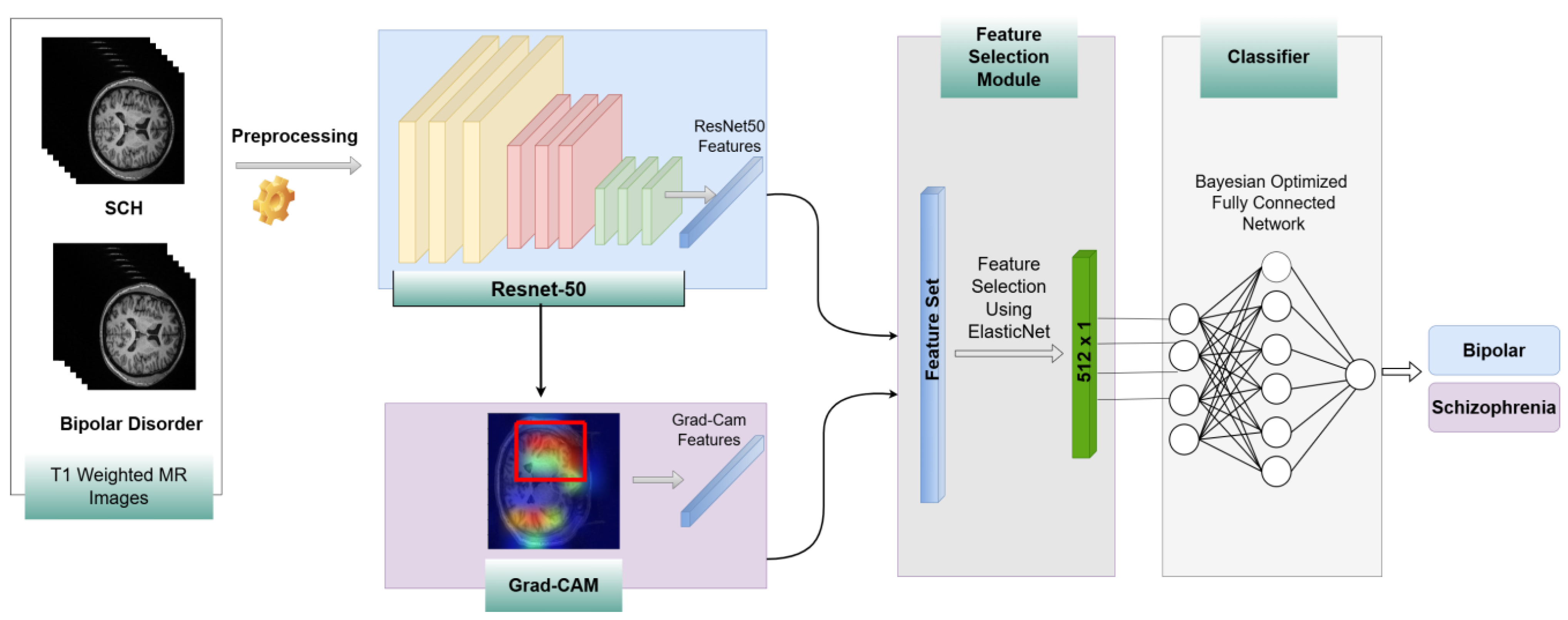
As illustrated in
Figure 2, the workflow begins with the training of a ResNet-50 model on MR images. After training a fine-tuned ResNet-50, we analyze it with Gradient-weighted Class Activation Mapping (Grad-CAM) to extract the important regions on MR images that mostly affect the prediction of bipolar disorder and schizophrenia. These important regions are used to extract features from MR images. The features derived from the Grad-CAM-identified regions were combined with the global features extracted from the ResNet-50 model. This comprehensive feature set was then refined through feature selection to retain only the most important features that contributed to performance improvement. For this purpose, ElasticNet was employed, leveraging its advanced architecture to identify and prioritize key features. The selected features were subsequently given as input into a deep neural network (DNN) whose hyperparameters were optimized using Bayesian optimization, ensuring robust and efficient final classification.
Let
denote an individual feature derived from a single MR image sample. Thus,
represents all the features obtained from an MR image. Features extracted from a single sample using the ResNet-50 model and region-based features derived from important regions identified by Grad-CAM, as shown in
Figure 2, can be represented by
and
where the sub-indices
and
correspond to ResNet-50 and Grad-CAM-based region features, respectively. Then, a feature fusion method is employed, and all features from a single sample are concatenated into a combined vector, denoted as
. To improve the system’s performance and reduce features that can increase computation time, we apply a feature selection method. After feature fusion, we employ the ElasticNet method on the concatenated features extracted from the ResNet-50 model and Grad-CAM-based features. By utilizing this method, we reduce the dimension of features from 2065 to 512 by applying feature selection, and the final features are represented as
. Finally, these selected features are fed into a Bayesian-optimized DNN to classify the psychological disorders.
ResNet: ResNet-50 is a residual network consisting of 50 layers, introduced by [
40]. Its primary innovation lies in the use of residual connections. The architecture of ResNet is composed of numerous residual blocks, each of which includes several convolutional layers. After the convolutional layers, batch normalization and rectified linear unit (ReLU) activation functions are employed. ResNet is distinguished from CNN by identity mapping, which is given by (1):
where
and
represent the input and the learned residual function, respectively. If a network grows deeper, accuracy can decrease because of vanishing or exploding gradients. The residual connections within the network help prevent issues related to exploding and vanishing gradients. Therefore, this structure allows the creation of deeper models.
The ResNet-50 model is widely employed for image classification tasks, and the pretrained ResNet-50 model is trained on a dataset of over one million images spanning 1000 different classes included in the ImageNet database. The size of the input images for the ResNet-50 architecture is 224 × 224.
Gradient-Weighted Class Activation Mapping (Grad-CAM): In recent decades, deep learning models have achieved significant success in handling image classification tasks. Although deep learning models can accomplish various tasks well, interpreting the results of the model is not always easy. Therefore, Grad-CAM, introduced by [
37], addresses this issue by providing a visual explanation of CNN predictions. These properties of the model allow researchers to understand which areas of an image are most responsible for the decision.
Mathematically, Grad-CAM computes a weighted sum of the feature maps, where the weights are the gradients of the score for the target class with respect to the feature maps [
37]. This process produces a localization map, emphasizing the areas in the image that contribute to the final decision of the network.
Grad-Cam uses the gradient information of the CNN. First, the gradients of the class score with respect to the feature map are computed as follows [
37]:
where
is the score for class
,
is the feature map, and
represents the indices of the feature map. After that, in order to determine the importance of the feature map
, gradients are globally average pooled as follows [
41]:
Here,
represents the size of each feature map, and the subindices
and
denote the position of
. The equation given above actually calculates the global average pooling of gradients via backprop. Finally, the heatmap is calculated as a weighted combination of the forward activation map. In order to obtain the final heatmap results, the weighted combination of maps is given as an input to the ReLU function. Let
denote the heatmap; then it is calculated as follows [
41], as shown in (4):
One of the major advantages of Grad-CAM is its applicability to a wide range of CNN-based architectures without altering the network’s structure. This flexibility makes Grad-CAM a valuable tool for explaining black-box models. In addition to enhancing interpretability, Grad-CAM has also been used in hybrid deep learning models to extract meaningful features from localized image regions, as accomplished in this study.
Feature Selection Module—ElasticNet: ElasticNet was used for feature selection in this study. This method incorporates the advantages of Lasso (L1 regularization) and Ridge (L2 regularization), making it particularly suitable for high-dimensional data. ElasticNet was proposed in [
42] and focuses on the limitations of Lasso by linearly combining L1 and L2 penalties. This approach is especially beneficial for feature selection tasks. ElasticNet accomplishes this task not only by shrinking coefficients to prevent overfitting but also by performing variable selection by reducing some coefficients to zero. In this way, non-essential features are eliminated from the model. The objective function in ElasticNet is defined as shown in (5):
where
controls the overall strength of the penalty,
determines the balance between L1 and L2 regularization (with
reducing ElasticNet to Lasso and
to Ridge), and
represents the coefficients of the predictors. By adjusting
and
, ElasticNet flexibly tunes the regularization to optimize feature selection for each specific dataset.
In this study, ElasticNet is applied as a feature selection tool, filtering out less informative features and retaining those that are most predictive. By setting the parameter appropriately, ElasticNet performs an effective trade-off between sparsity via L1 regularization and stability via L2 regularization. This feature selection process enables the model to focus on the most relevant features while reducing the dimensionality of the input space, thus enhancing both computational efficiency and interpretability. The ability of ElasticNet to handle collinear variables is important in complex datasets. This property of the model prevents redundant features from obscuring meaningful patterns. This also ensures that only the most powerful predictors contribute to the final model.
Bayesian-Optimized DNN: In this study, a Bayesian optimization method was used to determine the optimal architecture for a deep neural network. Bayesian optimization is an efficient approach for searching the global optimum of black-box functions that are costly to evaluate. It is particularly advantageous when the objective function lacks a closed-form expression but can be observed at sampled input values. Its effectiveness and versatility make it particularly well-suited for machine learning and deep learning tasks, including tuning hyperparameters of deep neural networks [
43]. Besides, employing Bayesian optimization increases the performance of traditional deep learning models [
43,
44,
45].
We used this method in order to select the number of layers, the L2 regularization values, the number of units in each layer, learning rates, and dropout rates. Besides, it allowed a systematic search of the hyperparameter space in order to find a model that provides a balance between complexity and generalization. By using the Bayesian optimization method, we designed the final DNN architecture, which consists of specific configurations, regularization values, and hyperparameters to obtain the best classification performance.
In the Bayesian optimization process, prior probabilities determine the initial assumptions about the hyperparameters before any data are observed. In this study, these probabilities were modeled as uniform distributions for the hyperparameters. According to the prior probabilities, the number of units in each layer was sampled from a discrete uniform distribution ranging between 32 and 512, with steps of 32, and the dropout rates were sampled from a discrete uniform distribution between 0.0 and 0.5, with steps of 0.1. On the other hand, the L2 regularization coefficient was sampled from a continuous uniform distribution between 0 and 0.3. Moreover, the number of hidden layers and the learning rate were sampled from a uniform distribution. The number of hidden layers ranged from 1 to 5, and the learning rate was selected from a set of predefined values . This uniform prior setup provides a balanced exploration of the hyperparameter space, allowing the model to systematically refine the search as the optimization progresses and posterior distributions are updated. This posterior updating is what enables Bayesian optimization to efficiently identify regions of the search space where the objective function, such as validation accuracy is most likely to improve.
The optimization criterion for this process is to maximize validation accuracy. To evaluate the effectiveness of the optimization, the error was calculated based on the validation accuracy for the best hyperparameter combination.
After employing the Bayesian optimization method, our model consists of 4 layers with 512, 256, 256, and 512 units, respectively. The DNN model begins with an input layer of 512 dimensions. This number represents the dimension of features at the output of ElasticNet after the feature selection block. The second layer consists of 256 units with ReLU activation and kernel L2 regularization set to . This layer is followed by batch normalization and a dropout layer with a 0.1 dropout rate. Both L2 regularization and dropout are used to prevent the overfitting problem.
The second layer includes 256 units. Here, the ReLU activation function and the same L2 regularization value of are used as in the first layer. Batch normalization and a dropout layer with a 0.1 dropout rate are used after the second layer. The third layer of the network has 512 units with the same L2 regularization value. After that, batch normalization and a dropout layer with a rate of 0.4 are again utilized.
The layer at the output of the network includes a single unit utilizing a sigmoid activation function. This activation function is especially appropriate for binary classification tasks. The Adam optimizer is selected as optimizer of the DNN model, and the learning rate of the optimizer is chosen as 0.001. We choose binary cross-entropy, which is compatible with the sigmoid activation function, as the loss function. As stated in our results, this Bayesian-optimized DNN architecture achieves higher accuracy and generalization across test sets than other classical methods
4. Results
In this study, all simulations were conducted on a PC equipped with an Intel i7-9750H CPU (Intel Corporation, Santa Clara, CA, USA) operating at 2.6 GHz, with 16 GB of RAM. For GPU-accelerated computations, the algorithms were executed using an NVIDIA GTX 1660 Ti GPU (NVIDIA Corporation, Santa Clara, CA, USA) with 6 GB of dedicated memory, enhancing computational efficiency, particularly for tasks requiring substantial processing power.
The dataset, denoted by
, consists of individual image samples
with corresponding binary labels
, where
. Here,
represents the total number of samples, which have a
standardized resolution. In our simulations, the dataset is divided into batches, and the batch size is selected as 32. On the other hand, the epoch number is chosen as 100. Moreover, the data is divided using the k-fold cross-validation method. Importantly, the test and training splits were created based on patients rather than individual images, ensuring that images from 10% of the patients were exclusively used as the test set in each fold. This approach better reflects real-world scenarios, where models are often required to generalize to entirely new patients rather than new images from patients already seen during training. According to this strategy, the value of
k is set to 10, such that each fold includes 5 schizophrenia and 5 bipolar patients in the test set, while the remaining patients are used for training. This strategy is similar to the approach described in [
25].
To improve the generalization of the model and prevent overfitting, a checkpoint was used to save the best-performing model based on validation accuracy. After training, the performance of the model is evaluated on the test set in terms of performance metrics such as accuracy, precision, recall, F1-Score, AUC, and Matthews correlation coefficient (MCC).
Accuracy is defined as the proportion of correctly classified samples to all samples. Let TP, TN, FP, and FN represent true positive, true negative, false positive, and false negative samples, respectively. Then, accuracy is given by
Precision is the ratio of TP samples to all samples predicted as positive by the model and is written as
. On the other hand, recall is the ratio of TP samples to actual positive samples and is expressed as
. The F1-Score is the harmonic mean of recall and precision, and it is important when the dataset is imbalanced, and is written as follows:
AUC represents the area under the receiver operating characteristic, which is the trade-off between the true positive rate,
, and the false positive rate,
. Finally, MCC is another performance metric, and it is very useful when the dataset is imbalanced. The MCC is written as
Data Augmentation: To enhance the generalizability of the model and prevent overfitting, a data augmentation method is employed on the training images using various transformation techniques. Although there are several transformation techniques used in image classification, not all of them are suitable for medical images. Therefore, the data augmentation techniques applied in this study were carefully selected to ensure they were suitable for medical images, avoiding any transformations that might distort the images. The selected augmentations, such as controlled rotation, flips, brightness adjustment, and rescaling, were chosen to enhance the diversity of the training data without damaging the anatomical or diagnostic integrity of the medical images.
The first augmentation technique is rotation. In this method, images were randomly rotated by a specific angle. In our study, we set the angle to a range between 0 and 30 degrees. This technique introduces rotational invariance, enabling the model to better handle variations in image orientation. Additionally, random horizontal and vertical flips were used to diversify the spatial orientation of the training data. On the other hand, brightness is adjusted to a value from 0.85 to 1.35, which supplies different lighting conditions to increase the adaptability of the model to different brightness variations. Finally, each pixel value was rescaled by a factor of 1/255 to normalize the input data of the model. This data augmentation approach increased the variability of the training dataset. By simulating a range of real-world variations, these transformations improved the robustness of the model and enhanced its generalization.
Model Workflow: The first model utilized in this study is based on the ResNet50V2 architecture. The ResNet50V2 model was initialized with pre-trained weights on the ImageNet dataset. We apply a fine-tuning strategy to train the network. For this purpose, we freeze the initial 75 layers of the ResNet50V2 architecture. This step ensures that the lower-level feature extractors, which capture general patterns such as edges and textures, remain intact and unchanged. By freezing these initial layers, the model can utilize the robust pre-learned features acquired from training on the ImageNet dataset. This also reduces the number of trainable parameters, leading to a more efficient training process and decreased computational cost.
Moreover, to adapt ResNet-50 to our problem, the model’s top fully connected layers were excluded, enabling the integration of custom layers to fine-tune the network. Specifically, a GlobalAveragePooling2D layer was added to reduce the feature map dimensions and to overcome overfitting. After that, we utilize a fully connected layer, which has 128 units, and a ReLU activation function. Besides, L2 regularization is utilized to increase the model’s generalization. A dropout layer is added to avoid the overfitting problem during training, and we set the dropout rate as 0.2. Then, the sigmoid activation function is used at the output layer of the network.
To train the model, we employ the Adam optimizer and choose the learning rate of the optimizer as 0.00005. On the other hand, the loss function is selected as the binary cross-entropy loss function, which is compatible with the sigmoid activation function at the last layer. The results obtained using fine-tuned ResNet-50 model are presented in
Table 1.
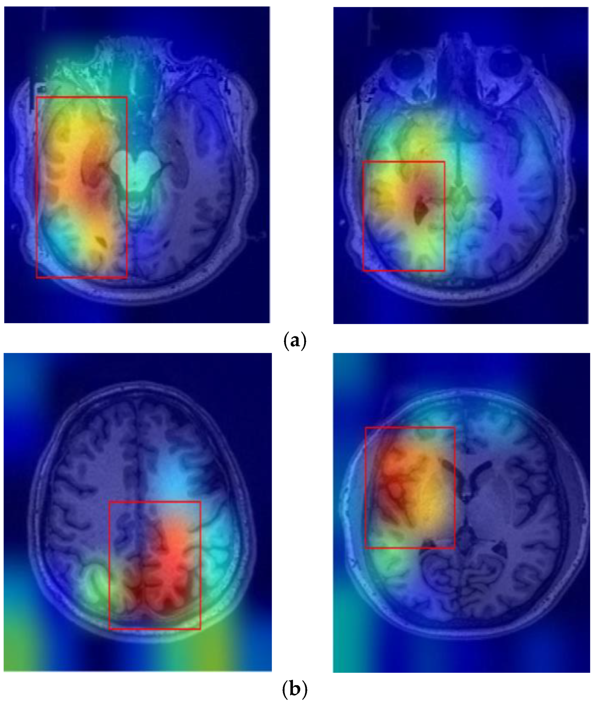
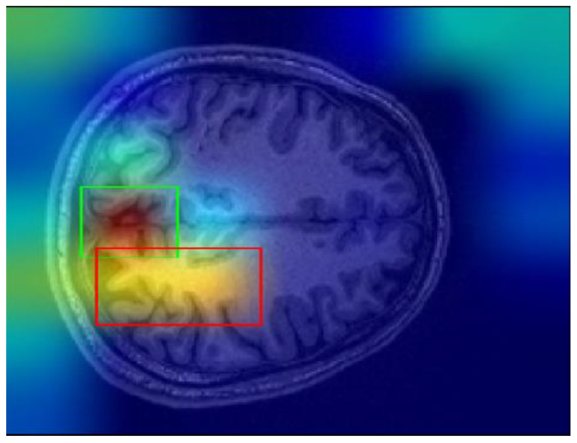
In this study, Grad-CAM was employed to identify the important regions in MR images that contributed most significantly to the classification of bipolar disorder and schizophrenia.
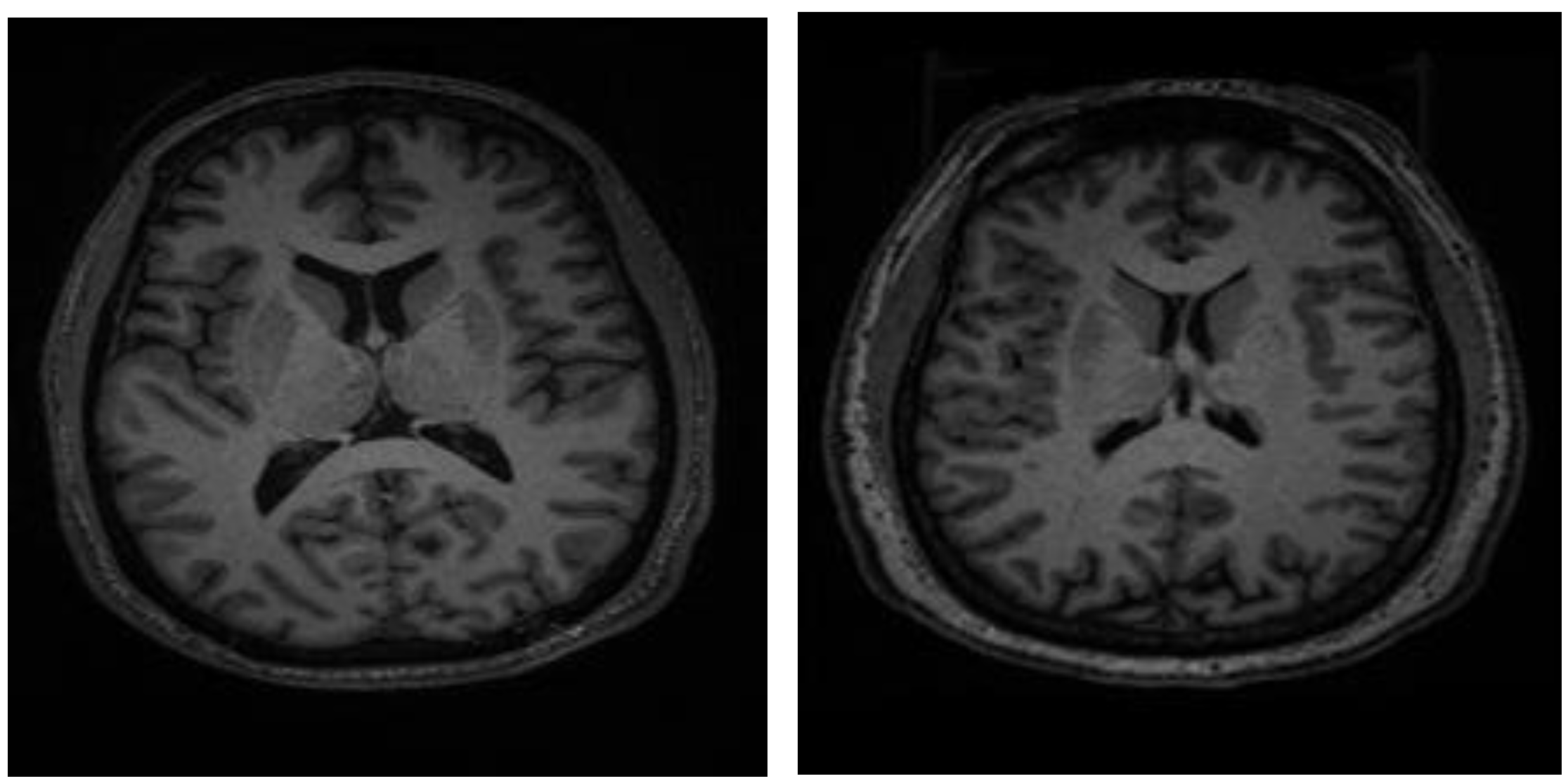
Figure 3a,b illustrates sample images from individuals diagnosed with SCH, bipolar disorder, and their corresponding Grad-CAM heatmap results. As shown in
Figure 4, the Grad-CAM heatmaps highlight the areas within each image that the model focused on during classification. After the heatmap is created, in order to identify the regions of interest highlighted by Grad-CAM, we apply a threshold value to the generated heatmap. If both red and green channel intensities exceed a value of 125, these areas are selected as important regions. This threshold value was determined through trial and error. In cases where two independent regions are identified, the region with the higher average intensity within its bounding box is prioritized as the primary area of interest. After that, we extract region-based features from the important areas determined by Grad-CAM. These features are area, centroid, eccentricity, orientation, extent, perimeter, solidity, major axis length, minor axis length, convex area, Euler number, and equivalent diameter. In addition to region-based features, statistical features such as minimum, maximum, variance, and entropy are also extracted from the important regions.
The performance of the proposed method is evaluated with various deep learning and machine learning models to classify bipolar disorder and schizophrenia. The performances of algorithms are evaluated in terms of precision, recall, F1-score, accuracy, and MCC metrics, and the results are given in
Table 1.
As seen from
Table 1, the fine-tuned ResNet-50 model achieved a precision of 76.64% for bipolar disorder and 79.60% for schizophrenia classification, with an accuracy of 76.77%. After that, we combine the features obtained from the fine-tuned ResNet-50 with Grad-CAM. Then, feature selection is applied to select the most important features. The selected features are used to classify bipolar disorder and schizophrenia. For this aim, first, SVM is employed for classification, and the model exhibited a lower overall accuracy of 75.19%. Secondly, we employed the XGBoost model in our problem, as given in
Table 1. The model achieved an accuracy of 76.27%. After that, the AdaBoost and RF algorithms are utilized, and they yielded overall accuracies of 75.88% and 76.73%, respectively. Although RF achieved a higher overall accuracy than other models, the performance of all models is close to each other.
The best classification performance is obtained by using the Bayesian-optimized DNN after employing feature selection. The accuracy of this model achieves a value of 78.84%. This model also outperforms other models, such as Support Vector Machines (SVM), AdaBoost, Random Forest (RF), and XGBoost in terms of all performance metrics. This indicates that Bayesian optimization effectively enhanced the model’s accuracy and predictive capability, outperforming traditional machine learning algorithms.
Furthermore, after performing feature fusion and feature selection processes, we achieved even more successful results compared to the ResNet model. The fusion and selection of features contributed significantly to enhancing model performance, underscoring the importance of dimensionality reduction techniques and optimal feature representation. These findings suggest that the tailored application of Bayesian optimization, combined with advanced feature engineering, can lead to substantial improvements in model performance, making it a promising approach for the classification of bipolar disorder and schizophrenia.
Figure 5,
Figure 6 and
Figure 7 illustrate the performances of models in terms of performance metrics.
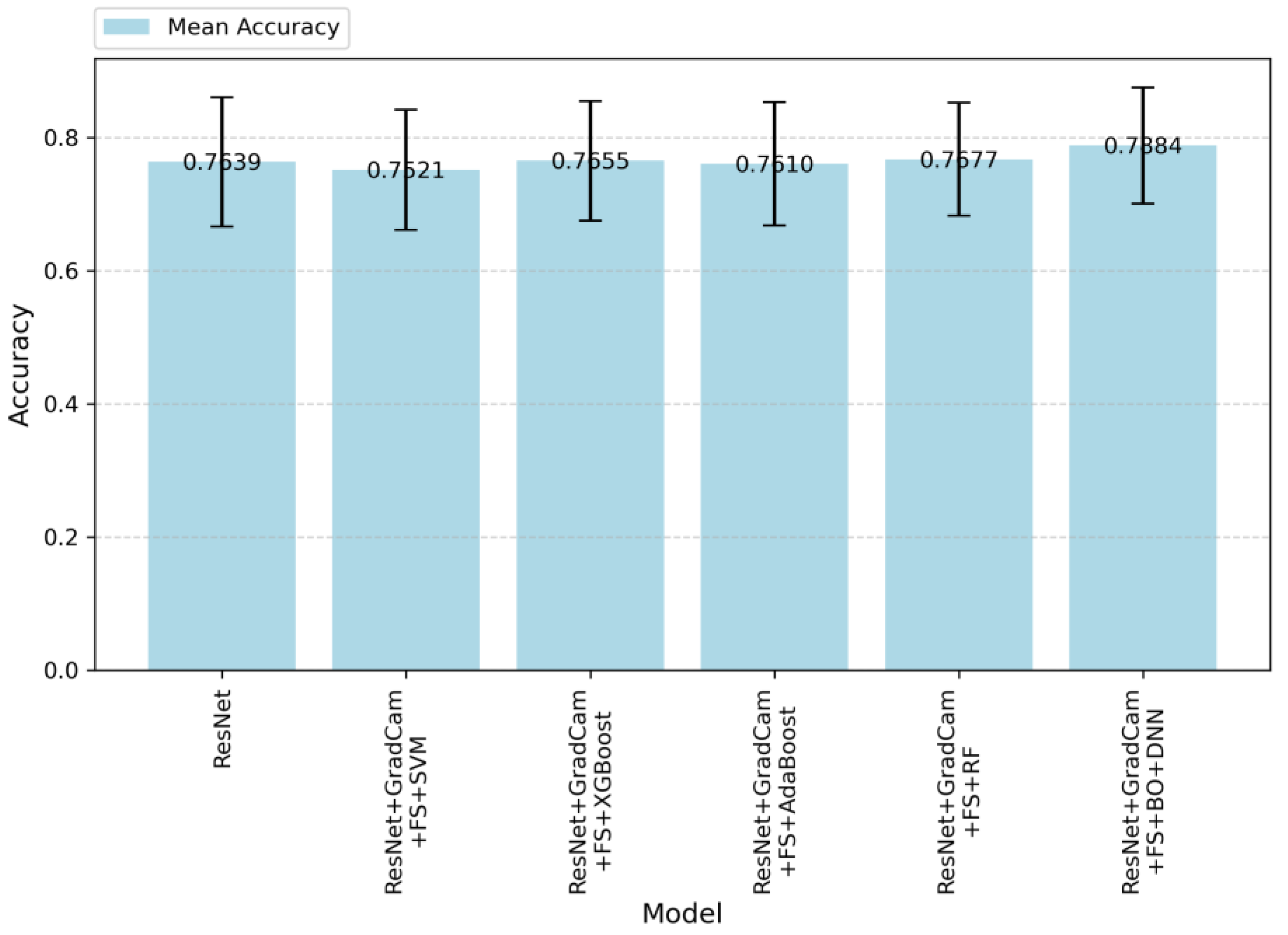
In
Figure 5, accuracy values are given according to the algorithms applied in this study. The results demonstrate an improvement as additional techniques are integrated into the baseline ResNet model. Althoug, the baseResNet model achieves moderate accuracy, the integration of feature selection, Grad-CAM, and advanced classifiers significantly enhances the performance. ResNet + Grad-CAM + FS + BO-DNN achieves the highest accuracy, indicating that this model effectively balances prediction precision and recall, thereby resulting in robust performance. On the other hand, the standard deviations of the models in terms of accuracy are similar. However, the ResNet + Grad-CAM + FS + BO-DNN model achieves both the highest maximum and minimum accuracy.
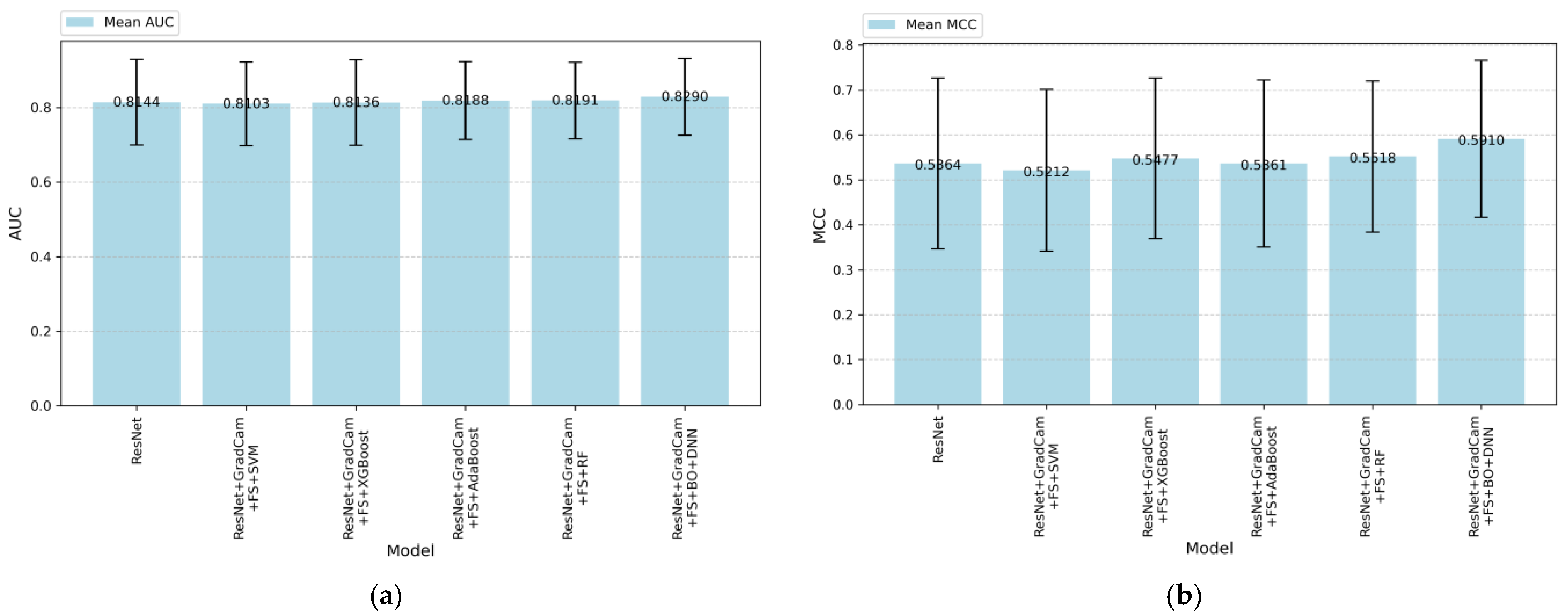
Figure 6 demonstrates the AUC and MCC performances for various machine learning and deep learning models. As shown in
Figure 6a, ResNet + Grad-CAM + FS + BO-DNN outperformed other models with a mean AUC of 0.890, followed closely by the ResNet + Grad-CAM + FS + RF model with a mean AUC of 0.891. The baseline ResNet model achieved an AUC of 0.844. On the other hand,
Figure 6b demonstrates the MCC performance of the models.
The ResNet model achieves an MCC score of approximately 52.77%. When ResNet is combined with Grad-CAM-based feature selection (FS) and traditional machine learning classifiers such as SVM, XGBoost, AdaBoost, and RF, there are minor performance improvements. Among these algorithms, RF achieves the highest MCC, which is 53.98%. The most significant improvement is observed with the combination of ResNet + Grad-CAM + FS + BO-DNN, which achieves the highest MCC score of 59.10%. This demonstrates a substantial improvement over both the baseline ResNet model and other hybrid configurations. The results highlight the effectiveness of using Grad-CAM feature extraction with the Bayesian optimization approach (BO-DNN) in combination with feature selection to enhance predictive performance.
On the other hand,
Figure 7 presents a radar chart that visualizes and compares the performance of all models in terms of performance metrics such as accuracy, AUC, precision, recall, F1-score, and MCC. The significance of this chart lies in its ability to provide an overall view of model performance by covering multiple metrics in a single visual representation. Each metric offers a unique perspective on the capabilities of the model. For instance, AUC and accuracy represent the overall classification ability, precision and recall highlight the balance between false positives and false negatives, F1-score captures the harmonic mean of precision and recall, and MCC evaluates the quality of binary classifications, especially for imbalanced datasets. The ResNet + Grad-CAM + FS + BO-DNN model stands out with the largest area in the radar chart, indicating superior performance in terms of metrics, indicating its strong generalization capability. This demonstrates that Bayesian optimization effectively tunes the deep neural network to learn robust features from the data. On the other hand, other configurations, such as ResNet + Grad-CAM + FS + RF, show competitive results in metrics like AUC and precision. However, the smaller overall area for these models suggests that their performance is less consistent across all metrics, highlighting potential trade-offs or limitations in certain aspects, such as recall and MCC. By combining these metrics,
Figure 7 highlights the importance of balancing performance across multiple dimensions rather than optimizing for a single metric.
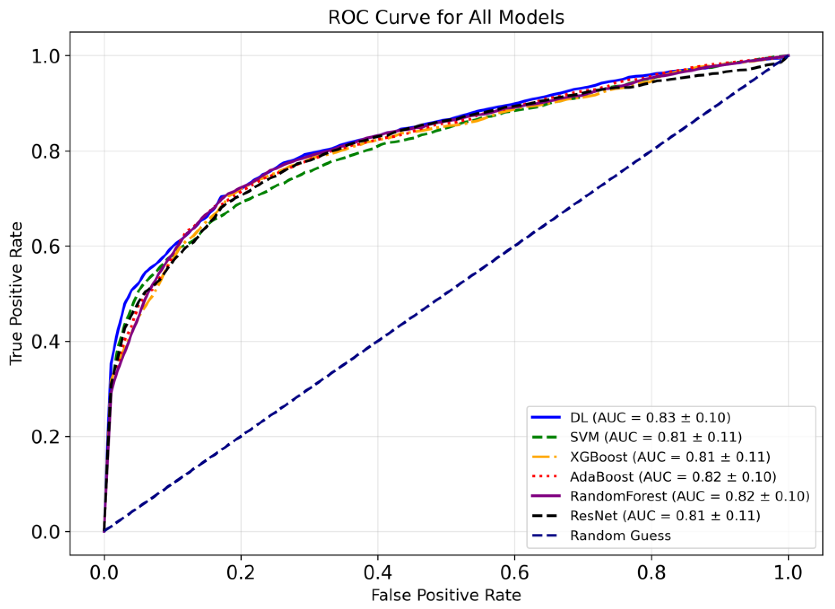
Figure 8 indicates the receiver operating characteristic (ROC) curves for the models employed in this study to classify bipolar and SCH disorders. As seen in the figure, the ResNet + Grad-CAM + FS + BO-DNN model achieves the highest mean AUC (0.83 ± 0.10), indicating its relatively better performance among the six models. On the other hand, AdaBoost and Random Forest demonstrate comparable performance to that of the BO-DNN model. SVM, XGBoost, and the baseline ResNet model achieve slightly lower AUC values, with minor differences among them. Moreover, the DL model demonstrates superior performance, especially in the lower false positive rate range (FPR: 0.0–0.2), as observed in its ROC curve. AdaBoost and Random Forest also exhibit consistent performance across all FPR values, demonstrating their effectiveness for this task.
Table 2 presents the comparison of various models in terms of AUC values provided in [
31] and the models proposed in this study. In [
31], the authors employed traditional methods such as 1D CNN, logistic regression (LR), support vector machine (SVM), linear discriminant analysis (LDA), Gaussian naive Bayes (GNB), k-nearest neighbors (KNN), decision tree (DT), and random forest (RF), and submitted their study to the IEEE Signal Processing Cup (SPC) 2023. As seen in the table, traditional methods generally exhibit moderate AUC values. They presented their results as public and private AUC values. For the competition, the AUC score was calculated as the average of the public AUC score, which was based on the public test set, and the private AUC score, which was based on the test set. It can be seen that 1D CNN achieves the highest AUC on both the public dataset and private dataset. However, the methods proposed in this study achieve higher AUC values than those reported in [
31] for the classification of BD and SCH. ResNet + Grad-CAM + FS + BO-DNN achieves the highest mean AUC, outperforming all other configurations. Additionally, this model attains the highest maximum AUC and the highest minimum AUC values in a test subset. On the other hand, ResNet + Grad-CAM + FS + XGBoost and ResNet + Grad-CAM + FS + AdaBoost also demonstrate competitive performance in terms of AUC.
Table 3 presents the results of paired
t-tests comparing the performance of various models against the ResNet baseline. The paired t-statistic,
p-value, mean difference, and Cohen’s d effect size are used to assess whether the differences in performance are statistically significant.
The ResNet + Grad-CAM + FS + BO-DNN model exhibited a statistically significant improvement over the ResNet baseline, with a paired t-statistic of −3.4337 and a p-value of 0.0089. The mean difference between these models was 0.0245 in favor of BO-DNN, and the Cohen’s d value of 1.1446 indicates a very large effect size, signifying a substantial performance advantage of this model over the baseline.
On the other hand, the other models did not show statistically significant differences when compared to ResNet. For instance, ResNet + Grad-CAM + FS + SVM reported a paired t-statistic of 1.2078 and a p-value of 0.2616. Similarly, ResNet + Grad-CAM + FS + XGBoost yielded a paired t-statistic of −0.1551 and a p-value of 0.8806, which also implies no meaningful improvement. Additionally, the paired t-statistics for these models ResNet + Grad-CAM + FS + AdaBoost and their associated p-values ResNet + Grad-Cam + FS + RF indicate that their performance differences relative to ResNet are not practically meaningful.
As shown in
Table 3, the Bayesian optimized model, ResNet + Grad-CAM + FS + BO-DNN, is the only model to show statistically and practically significant improvements over the ResNet baseline.
The statistical results given in
Table 3 are visualized in
Figure 9. These visualizations emphasize the significant distinction of the ResNet + Grad-CAM + FS + BO-DNN model compared to the other models.
Figure 9 shows the paired t-statistics for all models compared to the ResNet model. The t-statistics are plotted with their corresponding
p-values to show the statistical significance. The ResNet + Grad-CAM + FS + BO-DNN model demonstrates the largest negative t-statistic, which is associated with a statistically significant
p-value of 0.0089.
Figure 10 shows the t-distribution and highlights the critical regions for a significance level of
The vertical dashed lines denote the paired t-statistics for each model comparison against the ResNet baseline. Among the models, only ResNet + Grad-CAM + FS + BO-DNN falls within the critical region, with a t-statistic of −3.4337. The other models, such as SVM, XGBoost, AdaBoost, and RF, remain outside the critical region, and this indicates that other models have no significant difference from the ResNet baseline.
6. Conclusions
This study introduces an advanced deep-learning framework to address the diagnostic challenges posed by bipolar disorder (BD) and schizophrenia (SCH) using structural MRI data. The integration of ResNet-50, Grad-CAM, ElasticNet-based feature selection, and Bayesian-optimized deep neural networks (BO-DNN), which leverage explainability to extract features has demonstrated improved MRI analysis performance in classifying these psychological disorders compared to traditional machine learning methods.
The Grad-CAM technique enhanced model interpretability by highlighting diagnostically relevant brain regions, such as the prefrontal cortex, anterior cingulate cortex, and hippocampus. After highlighting the important regions for the decision-making process and extracting the features from these regions, the model’s performance in classifying BD and SCH was comprehensively evaluated using both spatial and morphological analysis. In this way, we obtained improved classification outcomes, as evidenced by the significant gains in accuracy and F1-scores. The success of the BO-DNN model underscores the importance of advanced optimization in achieving robust generalizability, making it a promising candidate for clinical applications.
Beyond improved diagnostic accuracy, the framework proposed in this study provides comprehensive insights, obtained from both quantitative and qualitative analyses, into key brain regions most relevant for differentiating these disorders. Furthermore, this novel approach overcomes the limitations of traditional methods, such as subjective assessments and reliance on overt symptoms. The results align with existing literature on the neuroanatomical distinctions of BD and SCH while providing additional insights into the structural underpinnings of these disorders.
However, there are certain limitations in this study. The reliance on a single open-source dataset, while effective for initial validation, may limit the generalizability of the findings. Future studies should focus on larger, multi-site datasets to ensure broader applicability. Additionally, incorporating longitudinal data could capture the progression of neuroanatomical changes, further enhancing the model’s clinical utility.
In conclusion, this study advances the role of deep learning in psychiatric neuroimaging, offering a robust, interpretable, and scalable framework to classify BD and SCH. The proposed methodology and deep learning-based framework improve diagnostic accuracy and provide insights into key neurobiological markers, paving the way for more objective, non-invasive, and early diagnostic tools. With continued refinement and validation, this approach holds significant potential to transform psychiatric diagnostics and support personalized treatment strategies.


