Assessment of Transport Value and Environmental Impact of Automotive Driving: A Physical-Action-Based Approach

Featured Application

The paper addresses the hitherto unsolved problem of assigning physically measurable value to automotive transport services and their ecological footprints.

Abstract

This paper is concerned with the problem of assigning, in a physically transparent way, value to automotive transport services and their related environmental impacts. We discuss the idea that the transport value of an automotive service can be measured in units of physical action, i.e., in terms of the physical entity that measures the effect of work performed within a specified physical process. It is further argued that from this action-based transport value, two dimensionless figures of merit (FOM), TV and ETV, can be derived, which can be used as cost factors in algorithms designed to optimize transport services and logistic networks.

1. Introduction

Mobility, i.e., the ability to move from one place to another, has always been a major concern in human history [1,2,3,4]. In the current age of globalization and world-wide trade, mobility has become an even greater concern than in former times. In view of the increasingly dense and inter-linked supply chains, it is of paramount importance to coordinate the traffic of raw materials, goods and human workforces in a way that is consistent with ever-tightening economic and environmental constraints [4].

The complexity of this task is easily demonstrated by reference to the widely studied “travelling salesperson (TSP) problem” [5,6,7,8,9]. As a demonstration case, we consider in Figure 1a a graph featuring four cities (vertices) with interlinking transport paths (edges) and associated cost factors (numbers associated with edges). With these cost factors in place, the famous TSP problem can be solved by devising an optimum path with minimum expenditure in resources that takes a salesperson from a first city A, successively through all other cities, and finally back home to A again. Similarly, by devising time as a cost factor, the shortest possible travel time can be determined. The TSP problem became an item of scientific interest in the early 19th century and subsequently turned into a subject of basic and applied research in the field of informatics, mathematics and complexity research [5,6,7,8,9]. The TSP problem is part of a larger class of combinatorial optimization approaches that are currently applied in the logistics field [10,11,12,13,14,15]. As exact solutions through exhaustive search often prove to be computationally intractable, specialized algorithms have been developed which quickly rule out many of all possible paths to obtain quick approximate answers.

A problem of considerable current interest is that road transport is very energy intensive, and that to date most vehicles are powered by internal combustion engines which emit large quantities of greenhouse gases (GHGs) which contribute to global warming. In the European Union (EU) in 2022, the transport sector accounted for 31.0% of final energy consumption, the highest share of final energy consumption ahead of households (26.9%), industry (25.1%) and services (13.4%) [16]. A similar expenditure on energy is also quoted for the US in which the contribution of the transport sector is estimated to be approximately 27% [17]. In a recent review [18], it is argued that “if logistics were a country, its contribution of 12% of energy-related CO₂ emissions would range third in the emission league table behind China and the US”. In view of this situation, the European Union has initiated its Green Deal Initiative [19,20] with the ambition to become the first climate-neutral continent in 2050 and to reduce the net GHG emissions by 55% relative to the year 1990. With this background in mind, the logistics sector will apparently be challenged by continually tightening environmental constraints and an increasing bureaucratic burden of regularly reporting progress along this line.

Key interest of the logistics scene are complex added value chains in which raw materials are converted into various intermediate products which, in turn, are assembled into final products, that are finally absorbed in consumer markets. As all intermediate steps take place in different geographical locations, this workshare results in a plethora of transport requirements with a concomitantly large energy consumption and environmental impact. Regarding the optimization of such interlinked transport chains, the approach of the logistic sector is basically a managerial one in which transport distances to be travelled are minimized and in which transport steps with zero or minimal payload are strictly avoided [12,13,14,15,18]. In contrast to the state of the art in logistics, the present paper is concerned with individual point-to-point transport steps that build up each added value supply chain. In concentrating on these elementary steps, our focus is on energy consumption and its concomitant impact on the environment relative to the transport value that is generated in these elementary steps. To arrive at a physically measurable entity of transport value, we resort to the famous Hamiltonian principle of least action, which has been one of the key cornerstones in the development of classical analytical mechanics [21,22]. In its original form, this principle states that a mass $M$, moving in an external force field, will move from a first point $A$ in 3d-space to a more distant point $B$ within a time ${\tau }_{AB}$ along a trajectory that minimizes the physical action $W_{AB}$ that had been generated upon travelling from $A$ to $B$. Physics teaches that this integral formulation of classical mechanics is mathematically equivalent to the widely known Newton’s equations of motion. While the Newton and Lagrangian differential equations are widely used to determine the trajectories of massive objects moving in external force fields, the Hamiltonian integral formulation is an eye-opener towards two other largely unemployed opportunities: Firstly, the Hamiltonian principle puts a value label on each particular trajectory that has been produced by a travelling object; and secondly, the Hamiltonian principle shows that transport values can be measured and enumerated in terms of units of physical action, i.e., in terms of the physical entity that measures the effect of work performed while carrying out a physical process, such as moving a mass $M$ from the first point $A$ to a more distant point $B$ in a time ${\tau }_{AB}$ (For more details see Appendix A and Appendix B).

Before applying the Hamiltonian principle to logistic problems, a few additional considerations are in order. Unlike in the Hamiltonian scheme, a vehicle of mass $M$, carrying a payload $m<M,$ is compelled to move along a man-made road that has seldom or never been designed to represent a trajectory of minimum action. In contrast to the Hamiltonian scenario, the motion of a vehicle is not driven by external forces but rather by forces internally generated within the vehicle and powered by energetic resources carried with the moving vehicle in the form of fuels. Upon following such man-made roads, driver actions are necessary to keep the vehicle on its chosen road, partly by adapting the vehicle’s motion to changing traffic conditions and partly to changes in road profiles, such as curves and vertical road excursions along the earth’s gravitational field. All these driver actions generate transport value that accumulates while the vehicle is moving and finally converges to a value of $W_{AB}$ that characterizes the value gained in the entire trip.

In carrying out this program, Section 2 presents a brief outline of the mathematics involved in this paper, while Section 3 and Section 4 consider some easily overseeable traffic scenarios that physically move a vehicle of mass $M$ and its payload $m$ along different kinds of trajectories. In these individual transport scenarios, we use Newton’s equations of motion to evaluate the physical actions $W_{AB}$ that are generated thereby. Secondly, we compare the resulting action values of $W_{AB}$ to the energies that had to be expended to initiate the respective transports, to maintain their motions and to bring the vehicles to rest at their destinations. Section 5 summarizes the lessons learnt in the different transport scenarios and it emphasizes the fact that the values of $W_{AB}$ can be turned into two dimensionless figures of merit (FOM) $TV$ and $ETV$, which represent the economic value of the individual transports and the ecological footprint that had been generated alongside. A final and practically very important result is that in an onboard measuring approach momentary values of $TV\left(t\right)$ and $ETV\left(t\right)$ can be continually derived from momentary readings of acceleration, speed and spatial orientation of the vehicles and summed up by integration to attain the overall values of ${TV}_{AB}$ and ${ETV}_{AB}$ at the end of each trip. The key encouraging conclusion is that both parameters can easily and continually be assessed inside a moving car by reading out GPS positions produced by widely used navigational systems and the outputs of micro-inertial sensor systems also widely available in modern cars to enable safety features such as providing dynamic stability control (ESP) in challenging traffic conditions and/or releasing airbags in emergency situations.

2. Money Value and Physical Value of Mechanical Motion

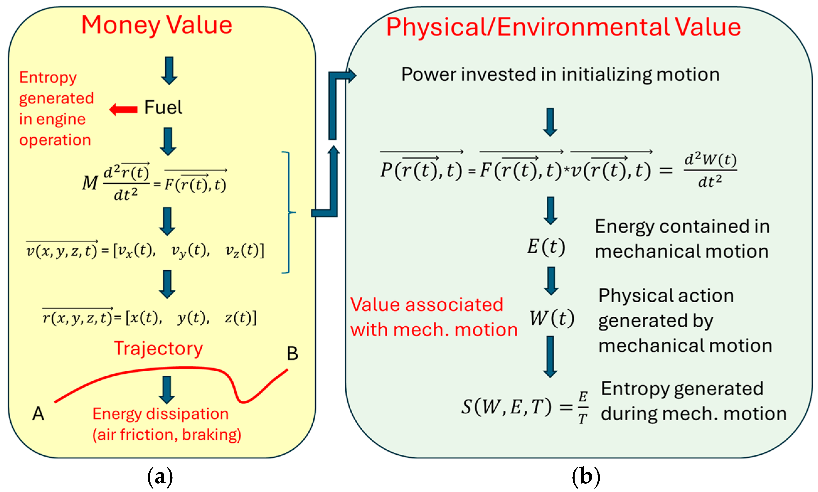
In this section, we present a shortcut through the mathematical considerations that are presented in the following sections. Secondly, we aim at discriminating between money values, which are man-made and often quantitatively incomprehensible, and physical values, which are derived from basic physical laws, and which thereby are free from disputable human imagination and interference. For the comfort of readers, the main ideas are summarized in the two sub-diagrams contained in Figure 2a,b.

Turning to Figure 2a first, it is shown that the process of initiating a point-to-point transport starts with buying a certain amount of fuel. This fuel contains a fixed amount of chemical energy that can be converted into mechanical motion using different kinds of engines. An unavoidable fact of life is that this conversion of chemical energy into mechanical energy always takes place with a finite efficiency $\eta <1,$ which means that right at the start, a fraction of the chemical energy is immediately converted into low-energy heat, from where it is no longer available for performing mechanical work. Whereas in the widely applied internal combustion engines $\eta =0.3-0.4,$it can take on values much closer to one in case electrical engines are employed. After this first step of energy conversion has taken place, we have left the realm of debatable money values, and we have entered a firm physical basis for evaluating the motional value of a moving car. Within the engine, the motional potential of the fuel is turned into engine power $P\left(t\right)$ and from thereon into forward-driving forces $F\left(t\right)$ through which the driver attempts to drive the vehicle along the chosen road. At the end of this process, the money value of the fuel has been converted into a geographically well-defined trajectory $\mathsf{\Gamma }(\overrightarrow{r},t)$, whose motional value, still has not yet been determined.

The process of assigning transport value to the generated trajectory is visualized in Figure 2b. Once the endpoint $B$ has been reached, all necessary engine power inputs ($P_i$) have been performed and the overall time variation of transport-initiating input powers, $P\left(t\right),$ is known. With the function $P\left(t\right)$ being known, the energy $E\left(t\right)$ spent up to point $t$ can then be determined by integration. In a second integration step, the energy consumption profile $E\left(t\right)$ is turned into a second function $W\left(t\right)$, which represents the physical action (in German, “Wirkung”, i.e., the effect of work done that leads to the trajectory $\mathsf{\Gamma }(\overrightarrow{r},t)$. Once the vehicle has arrived at its destination $B$ at the time ${\tau }_{AB}$, the trajectory has ended and the motional value $W\left({\tau }_{AB}\right)$ of the trajectory has been realized. Concomitantly, the kinetic energy spent up to this point had become totally dissipated and an associated ecological footprint has been generated inside the environment.

3. Some Simple One-Dimensional Transport Scenarios

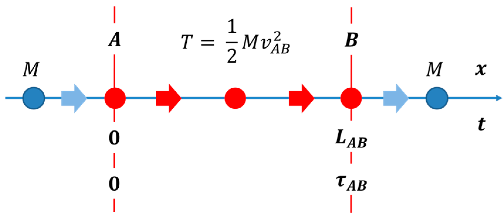
3.1. Idealized Fly-Through Scenario

In order to validate the idea of using the entity of physical action as a means of enumerating the physical value of mechanical motion, we consider a scenario in which a mass $M$ is moving with constant speed $v_{AB}$ along a straight-line path of length $L_{AB}$ connecting points $A$ and $B$ (see Figure 3). We further assume that this motion is perpendicular to the direction of the earth’s gravitational field. The potential energy $V$ of this mass can therefore be taken as a constant. In particular, we can set $V=0$ by choosing a Cartesian coordinate system in which the motion of the mass $M$ occurs along the x-axis and in which the direction of the gravitational field vector points along the negative z-axis. In the following section, we will call such a scenario a “fly-through” scenario.

In this highly idealized case, the kinetic energy of the moving mass is

$$T={\displaystyle \frac{1}{2}}M{v}_{AB}^2$$

(1)

and

$${\tau }_{AB}={\displaystyle \frac{L_{AB}}{v_{AB}}}$$

(2)

is the time required for traversing the distance $L_{AB}$ with speed $v_{AB}$. After traversing the length $L_{AB}$ with velocity $v_{AB}$, the change in the physical action $W_{AB}$ becomes:

$$W_{AB}\left(M,L_{AB},{\tau }_{AB}\right)={\int }_0^{{\tau }_{AB}}Tdt={\displaystyle \frac{1}{2}}M{v}_{AB}^2{\tau }_{AB}={\displaystyle \frac{1}{2}}M{v}_{AB}{L}_{AB}={\displaystyle \frac{1}{2}}M{\displaystyle \frac{L_{AB}^2}{{\tau }_{AB}}}$$

(3)

Reference to this latter result shows that the transport value of a mass $M$ is high, when the distance $L_{AB}$ is large and when this distance had been covered within a short time ${\tau }_{AB}.$This assignment of physical action as a measure of transport value is in line with the pragmatic approach to the problem of transport value, which normally assigns a high money value to long transport paths covered within a short time.

Accepting the function $W_{AB}\left(M,L_{AB},{\tau }_{AB}\right)$ as a valid measure of physical transport value, various efficiency measures can be defined. As a first measure, we consider the quantity of payload efficiency. This measure becomes relevant when a vehicle of mass $M$ transports a payload of mass $m\ll M$:

$${\eta }_{PL}(m,M,L_{AB},{\tau }_{AB})={\displaystyle \frac{m}{M}}{W}_{AB}\left(M,L_{AB},{\tau }_{AB}\right)$$

(4)

With this definition of payload efficiency in mind, the transport value of 1 kg of gold and 1 kg of bananas, transported by a truck of $10\mathrm{t}\mathrm{o}\mathrm{n}\mathrm{s}$ in weight, is the same and completely independent of the vastly different money values of both items. The physical value of transport, as defined by Equation (4), enumerates the value of delivering both goods, which are initially present at point $A$, to point $B$, which is separated from $A$ by a distance $L_{AB}$ and with a time delay of ${\tau }_{AB}$.

Another measure of efficiency with high practical relevance is the energy efficiency of transport:

$${\eta }_E(M,L_{AB},{\tau }_{AB})={\displaystyle \frac{W_{AB}\left(M,L_{AB},{\tau }_{AB}\right)}{E_{in}}},$$

(5)

where $W_{AB}\left(M,L_{AB},{\tau }_{AB}\right)$ is the transport value already defined in Equation (3), and $E_{in}$ is the energy that had to be expended to initiate the transport of mass $M$ over the distance $L_{AB}$ and in time ${\tau }_{AB}$. In the “fly-through example”, the value of $E_{in}$ obviously amounts to $E_{in}={\displaystyle \frac{1}{2}}M{v}_{AB}^2$, which was applied a long time before entering the transport path $\overrightarrow{AB}$ and which remained with the moving mass after it had crossed the distance $\overrightarrow{AB}$. Further, as no energy exchange between the transported mass $M$ and the environment had taken place within $\overrightarrow{AB}$, the energy efficiency ${\eta }_E(M,L_{AB},{\tau }_{AB})$ formally turns towards infinity, indicating the specific case of a zero-cost transport.

3.2. Start-Stop Scenarii

The “fly-through” scenario discussed above is an artificial one, only invented for motivating the entity of physical action as being a useful figure of merit for the hitherto undefined property of transport value. 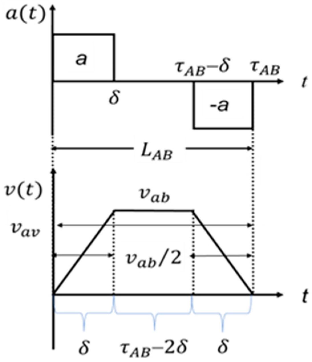Realistic transport scenarios distinguish from this highly idealized case in that usually, a mass $M$ starts out at point $A$ from rest, speeds up to a finite speed $v_{ab}>v_{AB}=L_{AB}/{\tau }_{AB}$ and slows down upon approach to its endpoint $B$, where it comes to rest again. In the following sections, we will call such point-to-point transport scenarios “start–stop transports”. Figure 4 displays the timing of the acting acceleration and deceleration forces across the entire transport duration ${\tau }_{AB}$.

For ${\tau }_{AB}$ to match the duration of the “fly-through transport” discussed in Section 3.1, accelerations $a$ and intermediate velocities $v_{ab}$ need to be adapted to the chosen lengths of the acceleration and deceleration phases $\delta$:

$$a\left(L_{AB,}{\tau }_{AB,}\delta \right)=\left[{\displaystyle \frac{L_{AB}}{{\tau }_{AB}\delta }}\right]{\displaystyle \frac{1}{1-\frac{\delta }{{\tau }_{AB}}}}$$

(6)

and

$$v_{ab}(L_{AB,}{\tau }_{AB,}\delta )=\left[{\displaystyle \frac{L_{AB}}{{\tau }_{AB}}}\right]{\displaystyle \frac{1}{1-\frac{\delta }{{\tau }_{AB}}}}.$$

(7)

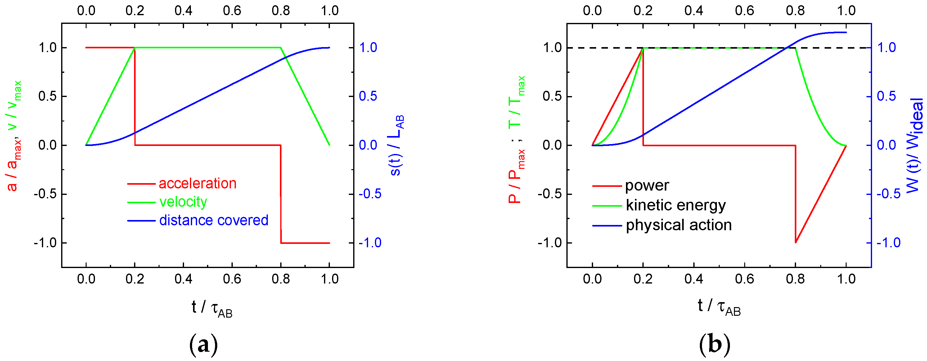
In Figure 5a, we show acceleration (red) and speed profiles (green), as well as the fractional distance $s\left(t\right)/L_{AB}$ covered up to time $t$ (blue), all as functions of the fractional transport time $t/{\tau }_{AB}$. In this first example, we assumed $\delta =0.2{\tau }_{AB}$. Figure 5b, on the other hand, shows the engine and brake power profiles (red) delivered to the mass $M$ close to points $A$ and $B$, as well as the resulting kinetic energy profiles $T\left(t\right)$ (green), both plotted once again against the fractional transport time $t/{\tau }_{AB}$. Also shown for comparison is the physical action $W(t,\delta )$ (blue) attained after time ${\tau }_{AB}$ and normalized to the physical action $W_{AB}(M,L_{AB},{\tau }_{AB})$ that had been attained at the end of the “fly-through” scenario in Section 3.1 above.

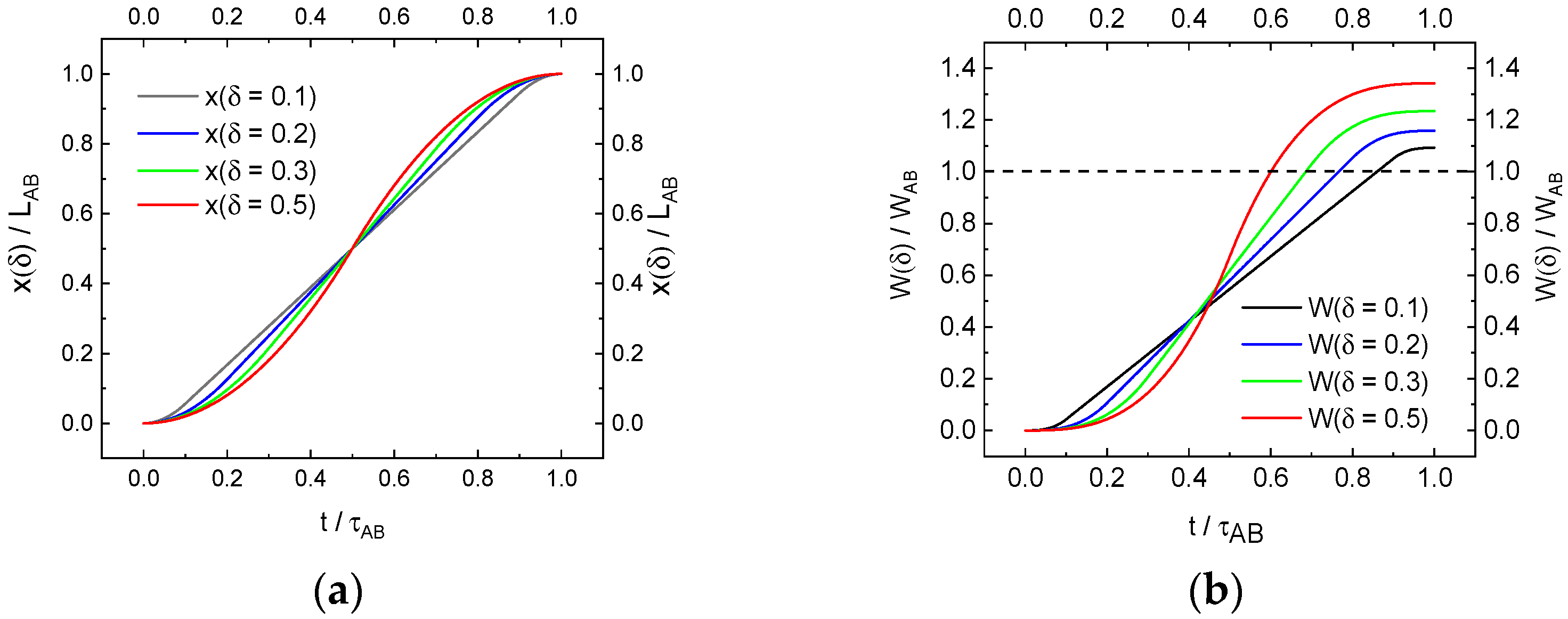
Figure 6a,b, in turn, plot the same quantities as above, however, for different lengths of acceleration and deceleration times. Figure 6a shows that longer acceleration and deceleration times lead to increasingly curvier distance-versus-time functions, with all functions increasing towards the same finally travelled distances. Figure 6b, on the other hand, shows that increasingly elongated acceleration and deceleration periods lead to increasingly larger final values of transport value $W_{AB}$. The considerations in Equations (8)–(10) show that this effect is related to the increasingly higher energy demands when $\delta ’\mathrm{s}$are increased.

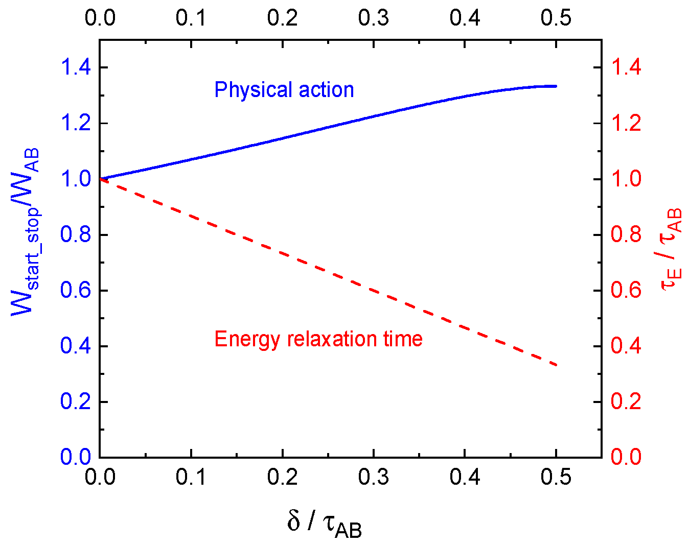
Quantitatively, the variation in $W_{start\_stop}\left(M,L_{AB},{\tau }_{AB,}\delta \right)$ with the acceleration and deceleration length $\delta$ is given by

$$W_{AB\_start\_stop}\left(M,L_{AB},{\tau }_{AB,}\delta \right)=W_{AB}\left(M,L_{AB},{\tau }_{AB}\right)\left\{{\displaystyle \frac{1-\frac{4}{3}\left(\frac{\delta }{{\tau }_{AB}}\right)}{{\left[1-\left(\frac{\delta }{{\tau }_{AB}}\right)\right]}^2}}\right\},$$

(8)

and drawn as a function of $\delta /{\tau }_{AB}$ in Figure 7.

Turning to the corresponding energy inputs and energy withdrawals, we note that the transport-initiating kinetic energy is

$$T\left(M,L_{AB},{\tau }_{AB,}\delta \right)={\displaystyle \frac{1}{2}}M{v\left(\delta \right)}^2={\displaystyle \frac{1}{2}}M{\displaystyle \frac{{\left[\frac{L_{AB}}{{\tau }_{AB}}\right]}^2}{{\left[1-\left(\frac{\delta }{{\tau }_{AB}}\right)\right]}^2}}.$$

(9)

Recalling that this same energy needs to be withdrawn again from mass $M$ as it approaches its destination $B$, the energy efficiency of the “start–stop scenario” becomes

$${\eta }_{E\_AB}\left(M,L_{AB},{\tau }_{AB,}\delta \right)={\displaystyle \frac{W_{start\_stop}\left(M,L_{AB},{\tau }_{AB,}\delta \right)}{T\left(M,L_{AB},{\tau }_{AB,}\delta \right)}}={\tau }_{AB}\left[1-{\displaystyle \frac{4}{3}}\left({\displaystyle \frac{\delta }{{\tau }_{AB}}}\right)\right].$$

(10)

This latter equation shows that the parameter of energy efficiency does no longer turn towards infinity as in the “fly-through scenario” above, but that it stays finite, matching the total transport time ${\tau }_{AB}$ when the transport-initiating energy is instantaneously introduced at point $A$ and instantaneously withdrawn close to point $B.$Extending acceleration and deceleration lengths $\delta$, on the other hand, towards $\delta ={\tau }_{AB}/2$, ${\eta }_{E\_AB}\left(M,L_{AB},{\tau }_{AB,}\delta \right)$ is lowered to ${\tau }_{AB}/3.$ Considering that the energy efficiency parameter ${\eta }_E$ takes on the physical dimension of time, the parameter ${\eta }_E$ can be regarded as an energy relaxation time ${\tau }_E$, which effectively measures the time during which the invested energy had stayed with the moving mass while it approached its destination $B$.

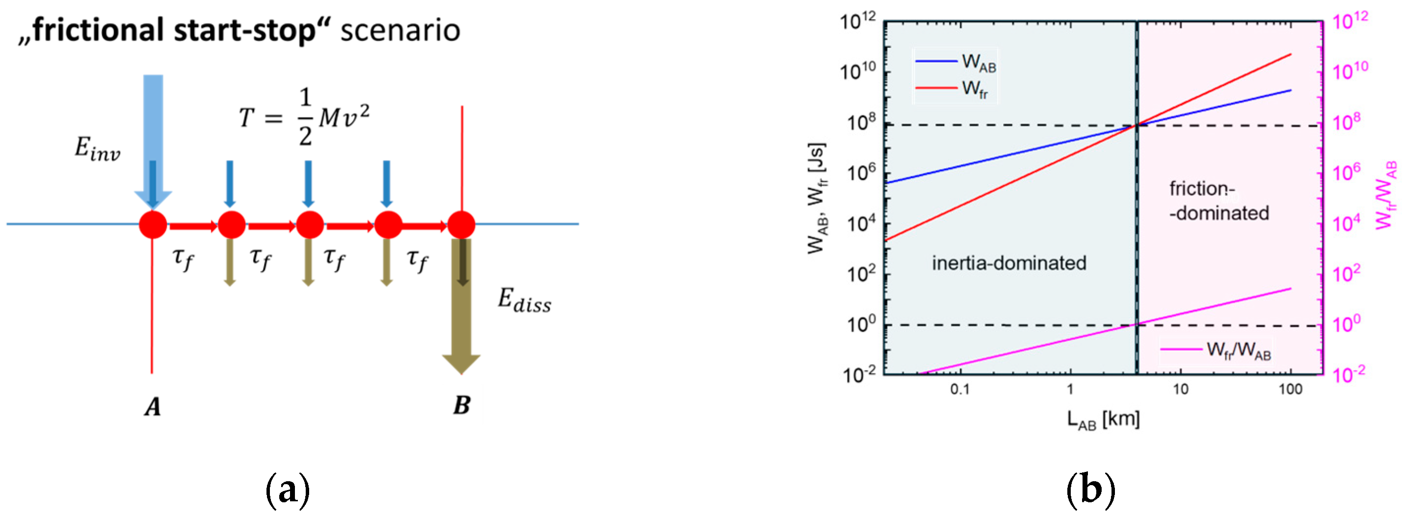
3.3. Frictional Transport Scenarios

The transport scenarios discussed above still represent highly idealized versions in that these completely neglect the effects of friction. In a friction-dominated transport scenario, acceleration and deceleration processes are the result of an interplay of forward-driving engine ($F_{en}$) and retarding frictional forces ($F_{fr}$), giving rise to a stationary velocity $v_{AB}$ (Figure 8a):

$$M{\displaystyle \frac{dv\left(t\right)}{dt}}=F_{en}-F_{fr}=0$$

(11)

In road-traffic situations, cars usually experience frictional forces that scale quadratically with the momentary speed $v\left(t\right)$ [23,24]:

$$F_{fr}\left(t\right)={{\displaystyle \frac{1}{2}}\varrho }_{air}A{C}_d{v\left(t\right)}^2.$$

(12)

In this equation, $v\left(t\right)$ is its momentary velocity, ${\varrho }_{air}$the air mass density, $C_d$ the dimensionless air drag resistance, and $A$the cross-sectional area of the vehicle.

Considering long transport distances $L_{AB}$ in which acceleration and deceleration phases close to start-points $A$ and endpoints $B$ do not play significant roles, engine power $P_{en}=F_{en}{v}_{AB}$ needs to be constantly applied to overcome the effect of air friction and to maintain a constant speed $v_{AB}$, as shown below:

$$P_{en}\left(v_{AB}\right)={{\displaystyle \frac{1}{2}}\varrho }_{air}A{C}_d{v}_{AB}^3.$$

(13)

Double integration over the transport time ${\tau }_{AB}$ first yields the energy input that is required for maintaining the speed $v_{AB}$ over the entire transport length $L_{AB}$ and then the physical action that is associated with the frictional transport over the length $L_{AB}$. With ${\tau }_{AB}=L_{AB}/v_{AB},$ the total energy input along the transport length $L_{AB}$ emerges as

$$E_{fr}\left(L_{AB},v_{AB}\right)={{\displaystyle \frac{1}{2}}\varrho }_{air}A{C}_d{v}_{AB}^2{L}_{AB},$$

(14)

and the generated transport value as

$$W_{fr}\left(L_{AB},v_{AB}\right)={{\displaystyle \frac{1}{4}}\varrho }_{air}A{C}_d{v}_{AB}{L}_{AB}^2.$$

(15)

With Equations (14) and (15), the energy efficiency of the frictional transport becomes

$${\eta }_{E\_fr}\left(M,L_{AB},{\tau }_{AB}\right)={\displaystyle \frac{W_{fr}\left(L_{AB},v_{AB}\right)}{E_{fr}\left(L_{AB},v_{AB}\right)}}={\displaystyle \frac{{\tau }_{AB}}{2}},$$

(16)

which shows that air friction reduces the energy relaxation time ${\tau }_{E\_fr}$ to a much shorter value than in the frictionless start stop–scenario with $\delta =0$, where it remained at ${\eta }_{E\_AB}\left(M,L_{AB},{\tau }_{AB}\right)={\tau }_{AB}$.

The supra-linear increase of $W_{fr}$ with transport length $L_{AB}$ and the smaller value of ${\eta }_{E\_fr}$ relative to the values of $W_{AB}$ and ${\eta }_{E\_AB}$ of the frictionless start-stop scenario (Equations (8) and (10)) reflect the larger energy expense of the frictional scenario for maintaining motion throughout the entire trip of length $L_{AB}$.

The most interesting aspect in the context with frictional motion arises when the length dependencies of the frictional and frictionless transport scenarios are compared. This is done in Figure 8b, which reveals a cross-over point between the frictionless and the friction-dominated “start–stop scenario” at transport lengths of around 4$\mathrm{k}\mathrm{m}$. This cross-over indicates that at shorter distances, inertial forces play a dominant role in requiring engine power inputs to initiate motion, while at larger distances, engine power requirements and associated fuel consumption are increasingly dominated by frictional forces. With regard to traffic optimization, this means that in the inertia-dominated domain, the generation of transport value is in the hands of drivers and their decisions of applying acceleration and deceleration forces, while in the friction-limited transport domain, the avoidance of excessively long transport distances and compliance with speed limitations are the parameters of choice that help to optimize transport values towards economic and environmental constraints.

4. Excursions Towards Higher and Lower Gravitational Potential Energy

So far, we have been dealing with one-dimensional transport scenarios that take place on an equipotential plane, i.e., in a direction perpendicular to the earth’s gravitational field. In this section, we turn to scenarios in which the transported mass $M$ takes excursions in the vertical direction, i.e., into directions along the earth’s gravitational field. Although the general reasoning about transport value and its energy cost remains the same, some important new features turn up, which are profile and control forces and the effect of path asymmetry.

4.1. Profile Forces

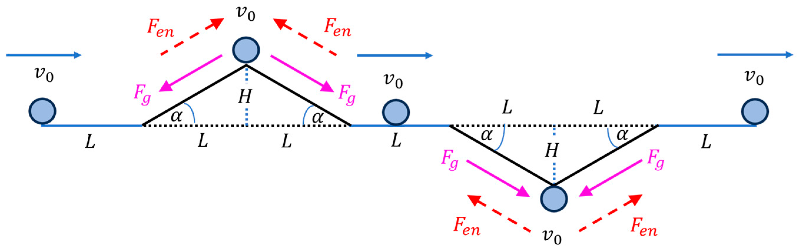
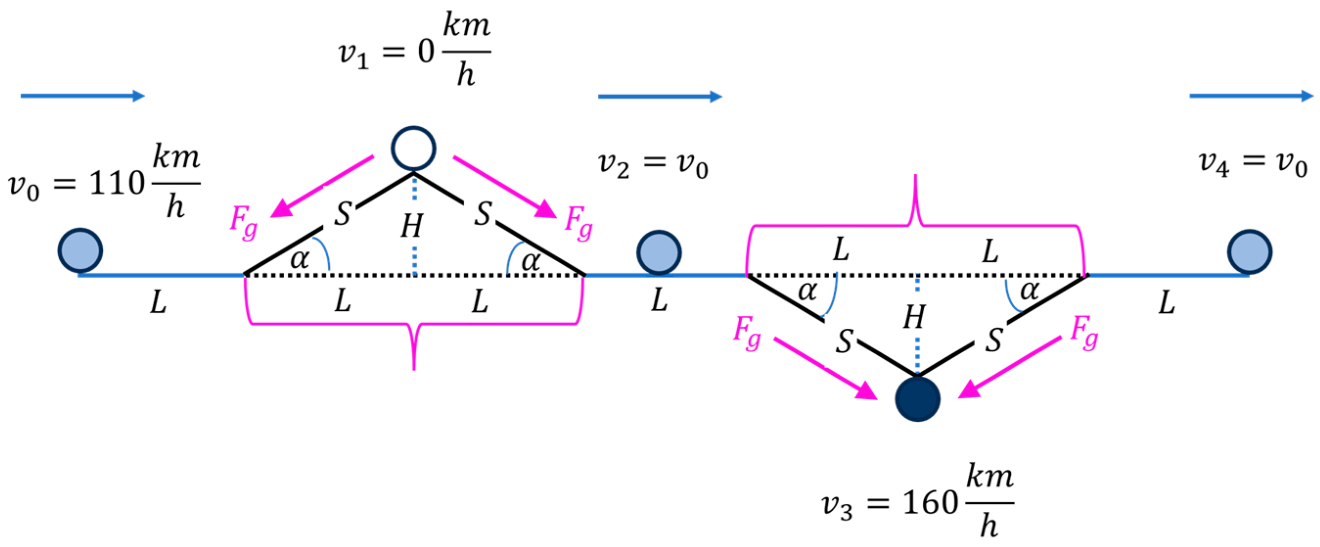
To start with, we consider in Figure 9 a frictionless road scenario in which a mass $M$ moves along a straight line across an equipotential plane, interrupted by an intermediate hill and a valley section. As shown in this figure, the entire road scenario consists of seven segments with individual lengths of $L=500\mathrm{m}$, which ensures that these segments are short enough to make inertial forces the dominating forces in the motion of mass $M$ throughout the entire road scenario. Within this scenario, the vertical extensions $H$ are limited to $H=50\mathrm{m}$, which limits slope angles $\alpha$ to practically occurring slope angles of about $6^{°}.$

With the assumed absence of air and wheel friction, frictionless transport through the entire scenario is enabled by supplying at start-off kinetic energy to mass $M,$ which is high enough to pass the summit of the hill section with zero velocity:

$${\displaystyle \frac{1}{2}}M{v}_{min}^2\ge MgH;v_{min}(H)\ge \sqrt{2gH}.$$

(17)

In this latter equation, $H$ is the summit height, $g$ the gravitational constant, and $v_{min}$ the minimum velocity upon start-up at point $A$. Starting with the minimum possible velocity of $v_0=\sqrt{2gH}~110{\displaystyle \frac{\mathrm{k}\mathrm{m}}{\mathrm{h}}}$ upon start-off, Figure 9 indicates that the summit of the hill section will be crossed with zero speed, while the bottom of the valley section will be passed with a high speed of $~160{\displaystyle \frac{\mathrm{k}\mathrm{m}}{\mathrm{h}}}$. Despite the zero net-energy expense associated with this travel mode, any responsible driver will not go through such extremes and rather apply engine and brake forces to arrive at a more constant speed throughout the whole trip.

The hill and valley sections represent “start–stop scenarios” with $\delta ={\tau }_{AB}/2$ and total length $2L$. Due to the sloping of the transport paths, sections of length $L$ are elongated to $S=L\sqrt{1+{\left(H/L\right)}^2}$. Gains in transport value upon crossing the hill section are as follows:

$$W_{profile}\left(M,v_o,L,H\right)={\displaystyle \frac{1}{3}}M{v}_{0}L\sqrt{1+{\left({\displaystyle \raisebox{1ex}{$H$}\!\left/ \!\raisebox{-1ex}{$L$}\right.}\right)}^2}.$$

(18)

Due to the regain of kinetic energy upon downward travel from the summit position, the energy efficiency turns towards infinity:

$${\eta }_{E\_profile}\left(M,v_0,L,H\right)={\displaystyle \frac{W_{profile}(M,v_{0}L,H)}{\left(-\frac{1}{2}M{v}_0^2\right)+\left(\frac{1}{2}M{v}_0^2\right)}}\to \infty .$$

(19)

Due to symmetry, the same results also apply to the valley section, revealing the hill- and valley scenarios as non-planar versions of “fly-through scenarios”.

4.2. Control Forces

Figure 10 highlights the same road scenario as displayed in Figure 9, however with the gravitational profile forces being compensated by additional engine forces. Due to the engine-enforced control forces, a constant and position-independent speed of $v_0$ is maintained. Due to the engine control, $v_0$ at start-off only requires $v_0>0$. Due to the engine control, the hill and valley scenarios feature slightly larger transport values and energy efficiencies than in the profile scenario above:

$$W_{control}\left(M,v_o,L,H\right)={\displaystyle \frac{1}{2}}M{v}_{0}L\sqrt{1+{\left({\displaystyle \raisebox{1ex}{$H$}\!\left/ \!\raisebox{-1ex}{$L$}\right.}\right)}^2}.$$

(20)

$${\eta }_{E\_control}\left(M,v_0,L,H\right)={\displaystyle \frac{W_{control}(M,v_{0}L,H)}{\left(MgH\right)+\left(MgH\right)}}={\displaystyle \frac{1}{2}}\left({\displaystyle \frac{v_0}{v_{min}^2}}\right)L\sqrt{1+{\left({\displaystyle \frac{H}{L}}\right)}^2}.$$

(21)

This latter result shows that the comfort and safety of driving at a constant speed involves both an economic and an ecological cost to be paid.

Figure 10. Road scenario as in Figure 9 above. Pink arrows denote profile forces of gravitational origin acting within the hill and valley sections. Broken red arrows denote engine-controlled, gravity-compensating control forces. Filled circles denote momentary positions of the transported mass. Speed indications denote associated momentary speeds.

Figure 10. Road scenario as in Figure 9 above. Pink arrows denote profile forces of gravitational origin acting within the hill and valley sections. Broken red arrows denote engine-controlled, gravity-compensating control forces. Filled circles denote momentary positions of the transported mass. Speed indications denote associated momentary speeds.

4.3. Moving Long Distances Towards Higher and Lower Locations

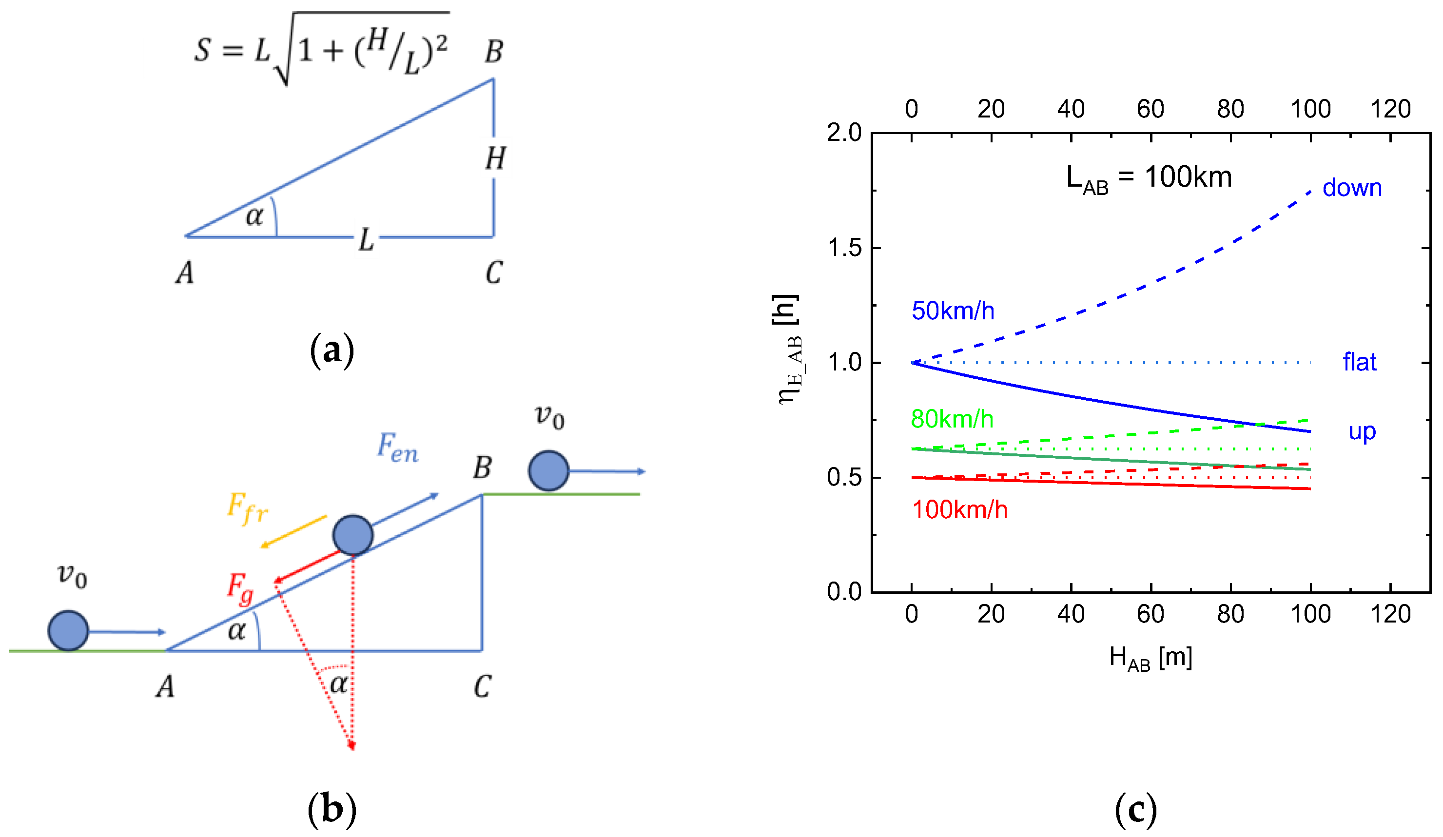
So far, we have been considering relatively short-range upward and downward excursions that require driver action, and which often result in additional fuel consumption. Considering journeys between two towns, $A$ and $B$, separated by lateral distances of say $L_{AB}=100\mathrm{k}\mathrm{m}$ and a constant upward or downward slope in between, the dominating effect in generating transport value and in determining fuel consumption is air friction.

Moving along the connecting road between towns $A$ and $B$, the trip is slightly elongated due to the road sloping (Figure 11a). The downward-dragging gravitational forces, on the other hand, need to be compensated by upward-dragging engine forces (Figure 11b). With both forces being compensated, the vehicle is effectively moving on a flat road, thus generating a transport value of

$$W_{fr\_AB}\left(M,L_{AB},H_{AB},v_{AB}\right)={\displaystyle \frac{1}{4}}{{\gamma }_{fr}v}_0{S}_{AB}^2,$$

(22)

where ${\gamma }_{fr}$ is a shortcut for ${\gamma }_{fr}={{\displaystyle \frac{1}{4}}\varrho }_{air}A{C}_d$. As the engine itself is left with the task of overcoming the effect of air friction and of lifting the vehicle to the higher location of B, the total energy demand is as follows:

$$E_{fr\_AB}\left(M,L_{AB},H_{AB},v_{AB}\right)={\displaystyle \frac{1}{2}}{{\gamma }_{fr}v}_{AB}^2{S}_{AB}+Mg{H}_{AB}$$

(23)

and the associated energy efficiency or energy relaxation time:

$${\eta }_{E_{fr}}\left(M,L_{AB},H_{AB},v_{AB}\right)={\displaystyle \frac{\frac{1}{4}{{\gamma }_{fr}v}_0{S}_{AB}^2}{\frac{1}{2}{{\gamma }_{fr}v}_{AB}^2{S}_{AB}+Mg{H}_{AB}}}.$$

(24)

In the limit of small height differences $H_{AB}$, the ecologically rated transport value for travelling from $A$ to $B$ become

$${\eta }_{E\_fr}(M,L_{AB},H_{AB},v_{AB})\cong {\displaystyle \frac{1}{2}}{\displaystyle \frac{S_{AB}}{v_{AB}}}+{\displaystyle \frac{Mg{H}_{AB}}{{\gamma }_{fr}{v}_{AB}^3}},$$

(25)

and

$${\eta }_{E_{fr}}(M,L_{AB},H_{AB},v_{AB})\cong {\displaystyle \frac{1}{2}}{\displaystyle \frac{S_{AB}}{v_{AB}}}-{\displaystyle \frac{Mg{H}_{AB}}{{\gamma }_{fr}{v}_{AB}^3}}$$

(26)

for the downhill travel from $B$ back to $A$. The sloping of the road obviously results in an asymmetry of the energetic cost for upward and downward traveling along the same road. Figure 11c shows that this asymmetry is large when travel speeds are relatively slow but decreases as average speeds are being increased.

5. Conclusions and Way Forward

The different transport scenarios discussed in Section 3 and Section 4 have shown that the physical entity of action is a useful measure for quantifying the amount of transport value that had been generated in an automotive ride. Additionally, the above considerations have paved the way towards two figures of merit (FOM) that measure (a) the economically relevant value of transport of the automotive ride, and which (b) provide an additional measure of the ecological footprint that had been generated alongside. While the first quantity of transport value had so far been measured in units of physical action, the second FOM of energy efficiency of transport value generation, or the equivalent energy relaxation time ${\tau }_{E\_AB}$, had so far been measured in units of time.

Discussing both FOMs regarding their relative importance and mutual trade-offs, it is advisable to turn both FOMs into dimensionless quantities and to give them suggestive names. Considering that automotive engine power is measured in kilowatts ($kW$) and travel durations in fractions of hours up to hours ($hr$), it is suggested to measure the physical action $W_{AB}$ generated in the transport in units of $kW{hr}^2$ and to name the respective FOM of transport value as:

$${TV}_{AB}={\displaystyle \frac{W_{AB}}{kW{hr}^2}}.$$

(27)

In this latter equation, the time unit of hours had been written as $hr$ to avoid confusion with the Planck constant $h$, which is the extremely small quantum of physical action. Being measurable in units of time, the second FOM of energy efficiency of transport value generation ${\eta }_{E\_AB}$, or energy relaxation time ${\tau }_{E\_AB}$, can be re-defined as ecologically rated transport value as:

$${ETV}_{AB}={\displaystyle \frac{{\eta }_{E\_AB}}{hr}}={\displaystyle \frac{{\tau }_{E\_AB}}{hr}}$$

(28)

The second definition of ${ETV}_{AB}$ in Equation (28) reminds us of the fact that the efficiency of transport value generation is related to the physical processes of energy dissipation and energy relaxation through which mechanical energy is degraded into heat, smog, greenhouse and poisonous exhaust gases.

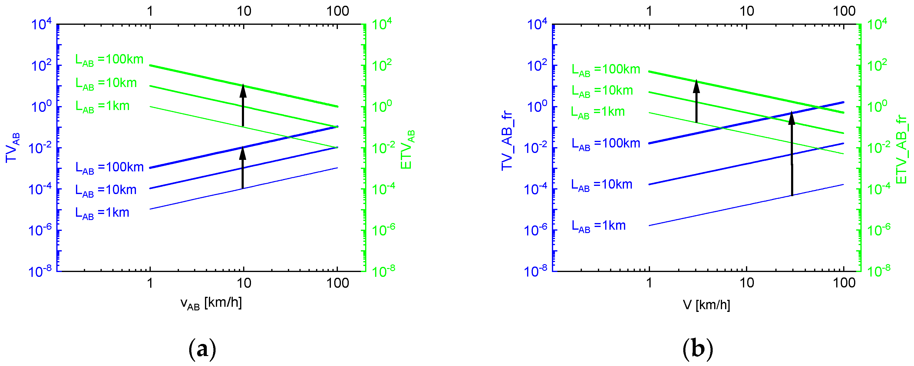
Starting with the discussion of both FOMs, we recall that there is a clear trade-off between the economic interest inherent in high values of ${TV}_{AB}$, on the one hand, and the ecological concern signaled by ${ETV}_{AB}$, on the other hand. While the first FOM measures the economic value of making goods and services, initially present at a point $A$, also available at a second point $B$, which is separated from $A$ by a distance $L_{AB}$ and with a time delay of ${\tau }_{AB}$, ${ETV}_{AB}$ represents a pure number that qualitatively enumerates the magnitude of the concomitantly generated ecological footprint. To show how ${TV}_{AB}$ and ${ETV}_{AB}$ scale with the distance $L_{AB}$ covered and the speed of transport $v_{AB}$ between start and endpoints, we have drawn up Figure 12.

More realistic than long-term transports at constant speed are frequent changes in momentary speed deriving from driver actions, such as adaptations to changing traffic situations, narrowly winding roads, or compensating for gravitational profile forces. Quantitative determinations of $TV$and $ETV$ in such situations require measurements of the temporal changes in ${TV}_{AB}\left(t\right)$and ${ETV}_{AB}\left(t\right)$ to obtain via subsequent integration values ${TV}_{AB}\left({\tau }_{AB}\right)$and ${ETV}_{AB}\left({\tau }_{AB}\right)$ that are representative of the overall travel from $A$ to $B$. While temporal changes in ${TV}_{AB}\left(t\right)$simply scale linearly with the momentary velocity $v\left(t\right)$,

$${\displaystyle \frac{d\left({TV}_{AB}\right({\tau }_{AB}\left)\right)}{dt}}~L_{AB}{\displaystyle \frac{dv\left(t\right)}{dt}},$$

(29)

the changes in ${ETV}_{AB}\left(t\right)$ vary in a more complicated way:

$${\displaystyle \frac{d{(ETV}_{AB}\left(t\right))}{dt}}~-{\displaystyle \frac{L_{AB}}{{v\left(t\right)}^2}}{\displaystyle \frac{dv\left(t\right)}{dt}}.$$

(30)

A common feature of both temporal changes is that determining the time variation of both FOMs requires the measurement of the momentarily acting acceleration $d\overrightarrow{v\left(t\right)}/dt$ inside a car. Such measurements are easy to perform due to the wide availability of micro-inertial sensors in cars. An example of a micro-inertial sensor chip is sketched in Figure 13.

Simple, one-dimensional acceleration sensors were first introduced into cars to trigger airbag safety systems (ABS). Later, multi-dimensional sensor systems, like the one shown in Figure 13, were introduced as key elements in ESP systems (ESP = electronic stability program), which sense the momentary motion of cars in three-dimensional space, and which apply brake forces to individual wheels to generate yaw moments that bring the car’s motion in line with the driver’s intention as signaled by measured steering wheel angles [30]. As the introduction of such systems into cars has significantly reduced the numbers of fatal car accidents, the introduction of such systems into cars has become mandatory via European and national legislations [31]. Modern cars, therefore, are comprehensively equipped with such systems, which in principle can additionally be used to determine momentary and time-integrated values of ${TV}_{AB}$ and ${ETV}_{AB}$. While online monitoring of both FOMs can give drivers immediate feedback on their performance as drivers, time-integrated values of ${TV}_{AB}\left({\tau }_{AB}\right)$and ${ETV}_{AB}\left({\tau }_{AB}\right)$, determined after completing a specific route joining start and endpoints $A$ and $B$, can provide valuable statistical data for the economic value and its associated ecological footprint of driving along a specified route. Frequently repeating such journeys along different routes within a specific area, can in the long run provide maps of FOM values, which represent averages over different traffic-, weather- and road conditions, and which can be used as cost factors in traffic and logistics optimization algorithms.