Article

An Advanced Model for Greenhouse Gas Emission Reduction in the Agricultural Sector to Achieve Sustainability for Thailand’s Future

by
Pruethsan Sutthichaimethee
1,2,3,
Phayom Saraphirom
1,2 and
Chaiyan Junsiri
1,2,3,*
1
Department of Agricultural Engineering, Faculty of Engineering, Khon Kaen University, Khon Kaen 40002, Thailand
2
Agricultural Machinery and Postharvest Technology Center, Khon Kaen University, Khon Kaen 40002, Thailand
3
Postharvest Technology Innovation Center, Science, Research and Innovation Promotion and Utilization Division, Office of the Ministry of Higher Education, Science, Research and Innovation, Bangkok 10400, Thailand
*
Author to whom correspondence should be addressed.
Appl. Sci. 2025, 15(3), 1485; https://doi.org/10.3390/app15031485
Submission received: 20 December 2024 / Revised: 25 January 2025 / Accepted: 29 January 2025 / Published: 31 January 2025
(This article belongs to the Special Issue The Transition toward Clean Energy Production 2024)

Abstract

:
This research aimed to develop an advanced model for sustainably reducing greenhouse gas emissions in the future. The research employs a quantitative research approach, introducing a new model called the Structural Equation Modeling with Vector Autoregressive Latent Trajectory Model (SEM-VALTM). This model differs significantly from previous models as it identifies strategic pathways for effective national administration, ensuring high performance without spurious results, surpassing the efficiency of earlier models. The findings reveal that the environmental sector is directly affected by the economic sector, with the relationship exhibiting an inverse direction. Similarly, the environmental sector is influenced by the social sector, also in an opposing direction. The SEM-VALTM model contributes new knowledge, highlighting that the environmental sector demonstrates the slowest adjustment toward equilibrium (6%). Under a sustainability policy framework, it was found that the economic sector, particularly the industrial rate, has the highest influence on economic changes, which in turn have the most significant negative impact on the environment. The study further projects that from 2025 to 2037, greenhouse gas emissions will rise sharply, reaching 95.05 Mt CO2 Eq., exceeding the carrying capacity threshold of 60.5 Mt CO2 Eq. Based on risk management principles, continuous measures must be implemented to reduce greenhouse gas emissions. Therefore, the government must establish a new scenario policy emphasizing renewable energy and clean technologies as substitutes. The findings suggest that future energy consumption will consistently decrease, resulting in greenhouse gas emissions of 50.04 Mt CO2 Eq. (2025–2037), which is below the carrying capacity.

1. Introduction

Countries worldwide have continuously pursued sustainable growth for the future, and Thailand is no exception. Thailand aims to advance towards Thailand 5.0 with a firm commitment to achieving the 17 Sustainable Development Goals (SDGs) [1]. A key focus is on SDG localization, which involves bringing global development agendas to local communities effectively [2]. Significant achievements include efforts to promote an integrated social protection system for all (Goal 1.3), addressing non-communicable diseases (Goal 3.4), providing inclusive education that encompasses migrant children (Goal 4.1), and promoting women’s political participation (Goal 5.5). Additionally, Thailand is empowering small and medium-sized enterprises (SMEs), fostering innovation among the youth with a focus on human rights in business, and transforming enterprises through digitalization (Goal 8.3). The country is also promoting inclusive economic growth that includes diverse gender identities (LGBTI) (Goal 10.2) and ensuring safe, legal, and orderly labor migration governance (Goal 10.7). In addition, Thailand has implemented climate change strategies (Goal 13.2), waste management initiatives (Goal 11.6), and a transition to green industries. This includes promoting low-carbon industries and supporting green finance and investment among SMEs (Goal 7.2). Furthermore, Thailand is enhancing inclusive citizenship to ensure broad access to citizen rights (Goal 16.9) and sharing best practices with other countries through South–South and Triangular Cooperation (SSTC) (Goal 17.9). These efforts aim to transform Thai society, ensuring prosperity, sustainability, and inclusivity for all sectors [1,3,4,5].
From 1990 to 2024, Thailand has achieved significant success in continuous economic development, despite facing an economic crisis in 1997. Thailand managed to overcome this crisis and resume steady growth, demonstrating the effectiveness of its economic policies and national governance [1,6]. This economic growth has also positively impacted the social sector, resulting in improvements such as universal access to education, comprehensive healthcare for all citizens, more efficient income distribution systems, and enhanced safety measures [2,3,7,8]. These achievements highlight Thailand’s strategic approach from the past (1990) to the present (2024), reflected in the implementation of the National Economic and Social Development Plans, from the 1st to the current 13th plan [9] (the Navigation of Thai Waterways Act, B.E. 2546, 2024). The objective has been to transition from a developing to a developed nation successfully, aligning with the Thailand 4.0 goals. Additionally, Thailand has outlined a 20-year national strategy (2018–2037) to fully realize the Thailand 5.0 vision. This strategy aims to maximize the country’s potential for sustainable and inclusive development [9,10,11,12].
Thailand is a country that relies heavily on the agricultural sector as its most important industry. The majority of the population has engaged in agricultural occupations from the past to the present. In recent years, economic development has driven higher growth rates, resulting in rapid expansion within the agricultural industry. As of 2024, agriculture has become the sector that contributes the most to greenhouse gas emissions in Thailand, with an increase rate of 69.05% (2024 compared to 1990). This continuous growth in greenhouse gas emissions has negatively impacted ecosystems and significantly contributed to climate change. Although Thailand has made substantial efforts to protect and conserve the environment, these measures have not successfully reduced the growth of greenhouse gas emissions. In fact, the former government was seen as lacking clear direction in addressing environmental issues and failing to provide the necessary tools for decision-making in the formulation of policies or measures. Additionally, when considering the sustainability policy framework, which requires simultaneous progress in the economic, social, and environmental sectors driven by political policies to achieve balance, it is clear that Thailand has not succeeded in transitioning towards the Thailand 5.0 vision [13,14]. This failure stems from an inability to adhere to sustainability policies. The environmental sector has experienced continuous deterioration, with ecosystems persistently damaged. As a result, greenhouse gas emissions have exceeded the country’s capacity to absorb them [14,15,16]. This ongoing degradation poses significant future risks, making the restoration of ecosystems unfeasible and leading to a state of unmanageable environmental decline.
Nonetheless, this research has developed a model to serve as a key tool in advancing strategies for sustainable national governance by reducing greenhouse gas emissions in line with the long-term national development plan set to conclude in 2037 [17,18]. In the past, no suitable model had been developed, and using an inadequate model for national strategy formulation could lead to significant errors. This research identifies the gap and has developed the right model, taking into account the causal factors from all sectors simultaneously. The model is designed to be adaptable for use in formulating future national strategies effectively.

2. Literature Reviews

The relationship between renewable energy consumption, economic growth, and CO2 emissions has garnered significant scholarly attention, revealing complex interactions that vary across regions, income levels, and institutional contexts. Wang et al. [19] demonstrated that while renewable energy consumption effectively curtails CO2 emissions in Sub-Saharan Africa (SSA), the agricultural sector amplifies emissions due to its energy-intensive practices. Governance quality emerges as a pivotal factor, capable of either mitigating or exacerbating these effects. Similarly, Kuldasheva and Salahodjaev [20] underscored the mediating role of institutional quality, finding that renewable energy reduces emissions in rapidly urbanizing nations. In the G-7 countries, Ike et al. [21] identified renewable energy consumption and higher energy prices as key factors in reducing emissions. However, trade activities exacerbate emissions, aligning with the Environmental Kuznets Curve (EKC) hypothesis, which posits that emissions initially rise with economic growth but eventually decline as countries reach higher income levels. Further evidence from OECD countries, as reported by Şanlı et al. [22], highlighted the long-term efficacy of renewable energy in reducing emissions, though its impacts are asymmetric compared to fossil fuels, which consistently increase emissions. In China, Riti et al. [23] validated the EKC hypothesis, showing that renewable energy reduces emissions over time despite short-term increases driven by economic and population growth. These studies emphasize the necessity of tailoring policies to specific regional and economic contexts to balance economic growth with environmental sustainability. Investigations into country-specific dynamics reveal additional complexities. Iqbal et al. [24] reported that changes in renewable energy production in Pakistan have asymmetric effects, with positive changes increasing emissions and negative changes reducing them over the long term. Similarly, Naz et al. [25] warned that foreign direct investment and unsustainable production practices can undermine the emissions-reducing benefits of renewable energy in developing economies like Pakistan. Alola and Joshua [26] have found that renewable energy improves environmental quality in the short term for low- and middle-income countries, but globalization produces mixed effects on emissions. Shaari et al. [27] observed that while renewable energy adoption supports emissions reduction, economic growth and a dependence on non-renewable energy present ongoing challenges to sustainability.
Recent studies have expanded the scope of analysis by incorporating additional variables, such as information and communication technology (ICT). Arshad et al. [28] highlighted the combined impact of ICT and renewable energy on reducing CO2 emissions in 21 Asian countries. Their findings reveal that while renewable energy and ICT adoption decrease emissions, factors like primary energy consumption, population growth, and industrialization exacerbate them. Raihan and Tuspekova [29], examining Malaysia, found that forested areas significantly mitigate emissions, while economic growth intensifies them. Renewable energy, though beneficial, has shown limited efficacy in reducing emissions, suggesting the need for a multifaceted approach that integrates sustainable forestry with renewable energy adoption. In SSA, Ansah et al. [30] illustrated the significant role of fiscal policy in shaping carbon emissions, with expansionary fiscal measures increasing emissions and contractionary policies reducing them. Renewable energy consumption alleviates emissions, whereas reliance on non-renewable energy exacerbates pollution. Similarly, Abdi [31] underscored the long-term benefits of renewable energy and economic complexity in enhancing environmental quality while identifying urbanization and economic growth as drivers of increased pollution. Transitioning to knowledge-intensive production systems and investing in renewable energy infrastructure emerge as critical strategies for the region. Complementarily, Pindiriri and Chidoko [32] noted the quadratic relationship between sustainable development assistance and emissions, emphasizing the importance of aligning external support with local capacities and priorities. Broadening the lens, Adendorff et al. [33] explored gender empowerment within South Africa’s renewable energy sector, proposing a socio-economic model that highlights the critical role of ethical leadership, targeted funding, and inclusive programs. Similarly, You et al. [34] examined the U.S. context, emphasizing how international collaboration in environmental technology fosters emissions reduction through domestic innovation and renewable energy consumption. Trade openness is highlighted as a key enabler, linking globalization with environmental progress.
Building on discussions of renewable energy, economic growth, and CO2 emissions, the application of forecasting models is crucial for predicting trends and supporting policy decisions in environmental and energy sectors. These models offer valuable insights into future scenarios, enabling more effective planning and mitigation strategies. For instance, Yu, Chang, and Ma [35] utilized computational fluid dynamics and the California Line Source Dispersion Model to simulate air quality, helping manage traffic congestion in urban areas and its associated emissions. In a similar vein, Sooktawee, Kanchanasuta, and Bunplod [36] applied a 24 h moving average to monitor hourly fluctuations in PM2.5, emphasizing its potential in guiding air quality control measures. Advanced techniques such as the autocorrelation error–informer model, presented by Cai et al. [37], have enhanced the accuracy of air pollutant forecasts, reducing errors when compared to traditional methods. These innovations in forecasting not only improve environmental monitoring but also offer essential tools for energy sector planning. Rehman and Deyuan [38] highlighted how forecasting models have informed energy strategies in Pakistan, helping bridge the gap between energy supply and demand. Likewise, Almuhtady et al. [39] employed statistical methods to connect electricity demand with weather variables, facilitating more efficient energy management. Additionally, Schrammel et al. [40] demonstrated how tailored consumption forecasts can enhance demand-side management by focusing on user behavior, suggesting that these models can play a pivotal role in optimizing both energy usage and emissions reduction. Together, these forecasting methodologies underscore the potential of advanced prediction techniques to inform sustainable practices, particularly in balancing economic growth with environmental sustainability.
Expanding on the previous discussions of forecasting models, several studies emphasize their application in energy transition strategies aimed at reducing carbon emissions and improving sustainability. Allen and Hammond [41] stressed the importance of accurate biomass usage projections in the UK’s bioenergy sector to meet carbon reduction targets. Similarly, Tilahun et al. [42] highlighted the optimization of Niger’s electricity mix, integrating renewable energy sources to balance both affordability and sustainability in the energy transition. In the context of off-grid areas, Awafo et al. [43] explored the potential of agricultural residues for rural electrification in Ghana, showcasing the role of forecasting models in identifying untapped resources for sustainable energy solutions. Moreover, Momodu et al. [44] analyzed low-carbon strategies for the electricity sector in West Africa, using forecasting tools to pinpoint key leverage points that can reduce emissions without compromising energy reliability. Zhu et al. [45] proposed a distributed energy network (DEN) for eco-city planning in China, underlining the role of forecasting models in the integration of renewable systems within urban infrastructure. Zhou and Chen [46] presented a novel forecasting method designed to predict China’s energy consumption and carbon emissions, aligning with the nation’s ambitious carbon neutrality goals for 2030 and 2060. Finally, Sahin and Chen [47] examined the impact of external events such as the COVID-19 pandemic on energy-related emissions in the United States, demonstrating how forecasting models can capture the volatility introduced by unforeseen events and their long-term effects on emission trends.
From the review of previous related studies, it was found that no research has successfully developed an appropriate model for reducing greenhouse gas emissions. This is because past models failed to consider validity. A model lacking the characteristics of the best model would result in significant errors and damage when used as a critical tool by the government for strategy formulation, potentially leading to irreparable consequences. Therefore, this research establishes an advanced model characterized as the right model, with the research process illustrated in Figure 1.
From Figure 1, the research process for developing the SEM-VAL model is illustrated. In this research, the following hypotheses were established:
  • The economic sector has a positively correlated influence on changes in the social sector.
  • The economic sector has a negatively correlated influence on changes in the environmental sector.
  • The social sector has a negatively correlated influence on changes in the environmental sector.
Based on these hypotheses, it can be inferred that government administration can achieve the goals of Thailand 5.0 and ensure long-term sustainability by analyzing the magnitude of the relationships among the three sectors, enabling them to grow together in harmony.

3. Material and Methods

The SEM-VALTM model introduced in this research is utilized to analyze the influences among factors categorized as exogenous latent variables and endogenous latent variables. Each factor comprises indicators known as observed variables. We have developed this model by applying advanced statistics, along with the relationship path of causal factors, which the model considers the most important principle, which shows the validity of the estimate results. It must have the highest reliability and reliability, which must not be spurious, have high performance, have white noise, and must have complete goodness of fit properties. The model is considered to have the characteristics of the best model. The purpose of the development of this model is to analyze the influence of relationships and create a national management strategy to achieve the Thailand 5.0 goal. In the past, Thailand lacked this type of model, and the models created in the past lacked such precautions. However, this model can be applied to all sectors and can be used publicly. We must select appropriate indicators for modeling and must be strict in conducting research at every step. If any step is found to not meet the criteria, that indicator must be immediately discarded, or the research must be restarted from the beginning. This must be repeated until the right model is created before it can be used for further analysis, detailed as follows [7,47].

3.1. Structural Equation Modeling Framework

For the data analysis in this research, the SEM-VALTM model was developed to analyze the influence of causal factors and to propose strategies for the administration of Thailand under the sustainability policy towards Thailand 5.0. The details of the SEM-VALTM model are as follows [17,47,48].
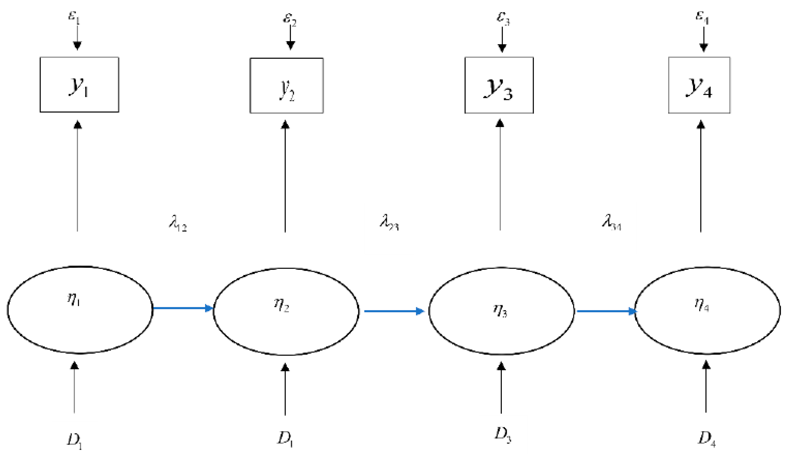
SEM-VALTM model: The SEM-VALTM model is a framework illustrating that the strength of relationships between variables diminishes as the time interval and differences between variables increase. In the context of longitudinal data analysis, this implies that the correlation of later measurements is lower than that of initial measurements, as shown in Figure 2 [16,48].
From Figure 2, the data analysis steps can be explained as follows [15,49]:
  • Model Specification: Define the model by specifying that the measurement score values must not have discrepancies. The parameter for the influence of true scores in the first measurement affects the true scores in subsequent measurements [49].
  • Identification of the Model: For any structural equation model, when analyzing to estimate parameters, the model must be identified to ensure that it is identifiable. A model is properly identified if the number of parameters to be estimated is fewer than the number of observed variable variance–covariance matrix members [15].
  • Parameter Estimation: Once identifiability is confirmed and the model is over-identified, the program estimates all model parameters. These parameters are then used to compute the variance–covariance values of the observed variables in the model.
  • Model Fit Assessment: Check if the hypothetical model aligns with the empirical data. In this research, the model fit indices considered include a non-significant chi-square statistic, the chi-square/degrees of freedom ratio χ 2 / d f should be less than 2, or less than 5 for more complex models; the Comparative Fit Index (CFI) and Tucker–Lewis Index (TLI) should be 0.90 or higher, preferably 0.95 or higher; the Standardized Root Mean Square Residual (SRMR) should be less than 0.05 for good fit and 0.05 to 0.79 for acceptable fit; and the Root Mean Square Error of Approximation (RMSEA) should be less than 0.05 for excellent fit, 0.05 to 0.07 for good fit, and 0.08 to 0.09 for acceptable fit [46,47].
  • Model Modification: Based on the analysis results, consider modifying the model by adding or removing influence paths that significantly reduce the chi-square value, enhancing the model’s fit with empirical data.
  • Parameter Estimation in the SEM-VALTM model with Latent Growth Variables—estimate parameters including factor loadings, means and standard deviations, and correlation coefficients [50].
For this model construction, only stationary data at the same level are used. Factors not meeting these criteria must be excluded or replaced using the Augmented Dickey–Fuller approach [51,52].

3.2. Spuriousness in the Analysis Results

For the SEM-VALTM model, it is essential to ensure the model passes both the goodness-of-fit and validity checks before it can be used for forecasting. In this research, issues such as heteroskedasticity, autocorrelation, and multicollinearity are addressed as follows [50,53].

3.2.1. Heteroskedasticity

Heteroskedasticity arises when the variance ( u i ) of the error terms is not constant and varies with the value of one or more independent variables (X¡) in the model. As the number of independent variables increases, the variance of the error terms tends to rise as well. This can be represented as follows [47]:
v a r u i = σ i 2
From Equation (1), heteroskedasticity arises from two primary causes: (1) the inappropriate selection of independent variables, where the model fails to select suitable independent variables, causing these variables to correlate with the variance of the error terms; and (2) the use of cross-sectional data, in which the non-constant variance of error terms is exhibited across observations, and each observation may have varying error term variances, leading to instability in the model.

Impacts of Heteroskedasticity

The variance of β ^ cannot be reliably used for confidence interval analysis. This is represented in Equation (2):
v a r β ^ = x i 2 σ i 2 ( x i 2 ) 2 A = π r 2
-
Lacks the property of efficiency, even though it possesses the properties of unbiasedness and consistency.
-
Hypothesis testing results are more likely to produce non-significance than normal.
-
Forecasted values exhibit higher-than-normal errors.

Detecting Heteroskedasticity

Heteroskedasticity can be tested using two methods: (1) The Graphical Method, where this method involves using graphs to examine if the variance changes as observations change. If the variance changes in the same direction as the observations, it indicates the presence of heteroskedasticity. (2) The Statistical Method, where this method includes tests, such as the Spearman rank-correlation test, the Goldfeld–Quandt test, the Glejser test, and White’s heteroskedasticity test. The most commonly used method is White’s heteroskedasticity test. As for this research, we have chosen to use White’s heteroskedasticity test to check the problem.

Methods for Resolving Heteroscedasticity

Heteroscedasticity is a common issue that can often be hidden within many models without researchers being aware of it. In reality, it can lead to significant errors. The method used in this research to detect heteroscedasticity is White’s heteroskedasticity test, which considers the Chi-square test ( n R 2 ) . If significance is found, it indicates the presence of heteroscedasticity, meaning that the variance of the error term is not constant. Therefore, if this issue arises, it is crucial to revise and improve the model. This research employs the Weighted Least Squares (WLS) method and further examines the value of n R 2 to check whether it remains significant. If it is found to be non-significant, it indicates that the model has been successfully weighted to resolve the heteroscedasticity problem.

3.2.2. Autocorrelation

Autocorrelation occurs when error terms are correlated with each other. This correlation can be of two types: positive autocorrelation (where error terms move in the same direction) and negative autocorrelation (where error terms move in opposite directions). This problem is typically encountered in time series data and is rarely observed in cross-sectional data. It can be represented by the following equation [46,52]:
E u i u j = 0
From Equation (3), it can be observed that the more the error terms are correlated with each other, the greater the impact on the accuracy of the equation. The causes of autocorrelation arise from three factors: (1) the inappropriate selection of independent variables, leading to error terms being correlated through these incorrect variables; (2) errors in defining the mathematical function or a misunderstanding of the principles involved; and (3) pure autocorrelation, arising naturally within the model itself.

Effects of Autocorrelation

-
The variance is not minimized, preventing the achievement of the efficiency property.
-
The model lacks consistency due to bias still present in the model.
-
Forecast values will exhibit higher-than-normal error rates.

Detecting Autocorrelation

Autocorrelation can be tested through several methods, with the most popular being the Durbin–Watson test. However, this test has limitations; it is appropriate only for data where the error terms exhibit a first-order regressive level. The model should present a conception value and should not be the first difference in the dependent variable (Lagged Dependent Variables). The testing procedure involves comparing the Durbin–Watson statistic to the critical values using the Durbin–Watson table, which shows the distribution of the statistic d ^ between d L and d U The results are interpreted as follows: ρ = 1 and d ^ = 4 indicates Perfect Negative Correlation, ρ = 0 and d ^ = 2 indicates Autocorrelation, and ρ = + 1 , d ^ = 0 indicates Perfect Positive Correlation.

Methods for Resolving Autocorrelation

The most severe case of autocorrelation is known as Pure Autocorrelation, which arises when the disturbance variables are correlated with one another. In this research, the Cochrane–Orcutt Iterative Method was selected to address the issue of autocorrelation. The process is carried out step-by-step, starting with the first-round residuals and then checking whether the problem still persists. If the issue remains, the process continues to the second-round residuals. However, if the problem cannot be resolved even after further iterations, the model must be revised immediately, as it will no longer be usable. The details of this process are as follows:
Y t ρ ´ ^ Y t 1 = α ρ ´ ^ α + β X t ρ ´ ^ β X t 1 + ε t *
From Equation (4), the error term is tested using the Durbin–Watson Test. If the test result allows for the acceptance of H 0 , it indicates that there is no autocorrelation, and the calculation process will stop. However, if the test result leads to the rejection of H 0 , it implies that autocorrelation still exists. Therefore, it is necessary to calculate the ε , ρ value at a higher order.

3.2.3. Multicollinearity

Multicollinearity occurs when independent variables are highly correlated with each other. The higher the correlation, the more it affects the model’s ability to explain the variation in the dependent variable. However, it is common for independent variables to exhibit some degree of correlation within the model. The issue arises when this correlation becomes strong enough to cause problems in the model. Specifically, if the correlation is imperfect multicollinearity, the model can still proceed; however, if it is perfect multicollinearity, it severely affects the analysis, leading to spurious relationships in the model. This can be represented as follows [53,54]:
X 1 i = α + β 2 X 2 i + ε i
From Equation (5), it can be observed that if a variable X X 1 i has a perfect relationship with another variable X 2 i , it will result in the inability to compute the values of the coefficients β ^ 1 and β ^ 2 . This is due to the determinant R 2 = 1 , and the values of S . E . E . ( β ^ 1 ) and S . E . E . ( β ^ 2 )   being equal to infinity. This makes ( X ´ X ) 1 a singular matrix, which prevents the calculation of the inverse. However, if the correlation is imperfect multicollinearity, the analysis may still proceed, but it will result in biased estimates, leading to potential forecasting errors.

Impact of Multicollinearity

The presence of multicollinearity can have significant impacts on the analysis, as it causes biased estimates, which affects the subsequent use of the model. The effects can be summarized as follows:
-
The correlation, r , will be high, which affects the analysis of the relationships.
-
Higher estimated values of S . E . E . β ^ 1 lead to reduced t-tests, resulting in the potential rejection of H 0 . If this happens, those variables should be removed.
-
The analysis cannot properly evaluate the model’s convergence toward equilibrium due to the high sensitivity of the variables.

Detecting Multicollinearity

Multicollinearity can be present in almost any model. There are several methods to detect it, with the most commonly used methods being: correlation coefficients, r , and Variance Inflation Factors, VIF, which can be calculated using this formula, V I F = 1 1 R 2 , as follows:
r = n X Y X Y n X 2 ( X ) 2 n Y 2 ( Y ) 2
From Equation (6), it can be observed that if the value r y , x is close to 1, it indicates that the dependent variable Y is highly correlated with the independent variable X , which benefits the model. However, if the independent variables are highly correlated with each other ( X i , X n ) , this will negatively impact the model and increase the likelihood of errors. As r x i , x n approaches 1, the problem of multicollinearity becomes more severe. Therefore, the researcher may need to add additional independent variables to the model or remove certain variables, depending on the appropriateness of the model [46,47].

Methods for Resolving Multicollinearity

The approach to resolving multicollinearity depends on the nature of each model. In some cases, researchers may not need to make any changes, as the unbiased properties of the model remain intact. However, in other models, it may be necessary to modify certain independent variables or add additional independent variables to the model. It is essential to consider the type of multicollinearity present. If it is Perfect Multicollinearity, this indicates that two or more independent variables in the linear equation model are completely correlated with one another. In such cases, it is necessary to examine and revise the independent variables, as the system will not be able to proceed otherwise. An example equation is provided below:
X 1 i = α + β 3 X 3 i + ε i
From Equation (7), if variable X 1 i is perfectly correlated with another variable X 3 i , this results in an inability to calculate the values of β ^ 1 and β ^ 3 . Additionally, S . E . E . ( β ^ 1 ) and S . E . E . ( β ^ 2 ) would be equal to infinity, because the ( X ´ X ) 1 matrix becomes a singular matrix, making it impossible to calculate its inverse. Therefore, the researcher must revise and reconstruct the model from the very beginning. Furthermore, if the relationship is classified as Imperfect Multicollinearity, a situation where the multicollinearity is high but not to the extent of Perfect Multicollinearity, this is due to the presence of a random variable δ i An example equation illustrating this is shown as Equation (8):
X 1 i = α + β 3 X 3 i + δ i
From Equation (8), one method to resolve the issue of multicollinearity is a straightforward approach, either modifying some of the independent variables or adding new independent variables to the model. However, the choice of method depends on the suitability of each specific model.

4. Empirical Analysis

4.1. Screening of Influencing Factors for Model Input

For this research, the SEM-VALTM model was developed by specifying three latent variables: economic, social, and environmental variables. In selecting the indicators to serve as the observed variables for explaining each latent variable in this model, indicators have been utilized based on Thailand’s national policies, which have guided the country’s management in the areas of the economy, society, and environment from the past to the present. For constructing the SEM-VALTM model, secondary data from 1990 to 2024 were employed. These data were sourced from government agencies responsible for data collection to determine the indicators. Each agency was required to prepare information under its jurisdiction in accordance with the sustainability policy. The indicators were assigned rates standardized to a common unit, enabling the data to be used for research, further studies, and as critical information for policy and planning decisions in Thailand. The indicators were designed to support the formulation of strategies and administrative plans for the country in the short, medium, and long term. This ensures the data are used accurately and appropriately. By standardizing the units of measurement for all indicators, the results of any calculations derived from the data are ensured to be as accurate and reliable as possible. For this research, the indicators were prepared as observed variables for each latent variable, as follows:
  • Economic Sector: The organization responsible for preparing and collecting the data is the Office of the National Economic and Social Development Council (NESDC). In this research, the following indicators have been utilized: the industrial structure rate ( I N ) ; per capita GDP rate ( Y ) ; qual foreign tourist rate ( F t ) ; urbanization rate ( U r ) ; indirect foreign investment rate ( I f ) ; total exports rate ( E M ) ; and government expenditure rate ( G e ) .
  • Social Sector: The organizations responsible for preparing and collecting the data are the National Statistical Office and the Ministry of Information and Communication Technology. In this research, the following indicators have been utilized: the consumer protection rate ( S c ) ; social security rate ( S e ) ; employment rate ( E s ) ; and health and illness rate ( H r ) .
  • Environmental Sector: The organization responsible for preparing and collecting the data is the Department of Alternative Energy Development and Efficiency. In this research, the following indicators have been utilized: the consumption rate ( E e ) ; green technology rate ( E g ) ; renewable energy rate ( E i ) ; and carbon dioxide emissions ( C O 2 ) .
Thailand has established a national strategy that includes the formulation of a sustainability policy. Under this policy, three key organizations have been designated to collect and prepare indicator data. These three agencies are responsible for compiling the data and calculating the rates as specified. This ensures that the data related to the economy, society, and environment are standardized and utilize consistent units across all domains. Such data have been designated for use in developing various models. In the past, Thailand has utilized these data in models such as the ANN model, MARP model, GB model, Gray model, and ARIMAX model. Accordingly, this research employs secondary data, designated as reliable and appropriate indicators, to develop the SEM-VALTM model. This model is designed to analyze the influence of relationships and to facilitate forecasting for future applications.
For the SEM-VALTM model, the researcher selected only stationary indicators. To ensure this, the Unit Root Test was conducted at level I(0) and the first difference level I(1) following the Augmented Dickey–Fuller (ADF) theory, as shown in Table 1.
From Table 1, it was found that all indicators are non-stationary at level I(0), as the Tau test values were less than the MacKinnon Critical Value at a statistical significance level of α = 0.01. For this research, only variables that were stationary at the same level were selected. Any variable that did not meet this criterion was immediately excluded from the model. To address this, all indicators were adjusted to become stationary by applying the first difference at level I(1). After this adjustment, it was found that all indicators became stationary at the first difference level I(1), as all Tau test values exceeded the MacKinnon Critical Value, leading the researcher to reject the null hypothesis. This indicates statistical significance at the first difference level. Therefore, the researcher utilized all the adjusted indicators at the first difference level I(1) to analyze long-term relationships by applying the Johansen and Juselius co-integration test, as shown in Table 2.

4.2. Analysis of Co-Integration

In this research, only indicators that are stationary at the first difference level (I(1)) were selected for the co-integration test based on Johansen and Juselius’ theory. Under the established hypothesis, if the analysis results in a rejection, this indicates that there is statistical significance, which makes it suitable for further application. The results of the analysis are presented in Table 2.
From Table 2, it was found that all indicator variables exhibit co-integration. At the None point, the trace test value was 255.01, and the Max-Eigen Statistic Test value was 201.05, both of which are higher than the MacKinnon critical values, indicating statistical significance at the level of α = 0.01. At Most 1, the trace test value was 85.00, and the Max-Eigen Statistic Test value was 81.01, both of which are higher than the MacKinnon critical values, indicating statistical significance at the level of α = 0.01. The results of the analysis show that all the indicators tested for co-integration have long-term relationships. Based on these properties, it is appropriate to use them to construct the SEM-VAL model to analyze the long-term magnitude of influence.

4.3. Formation of Analysis Modeling with the SEM-VALTM Model

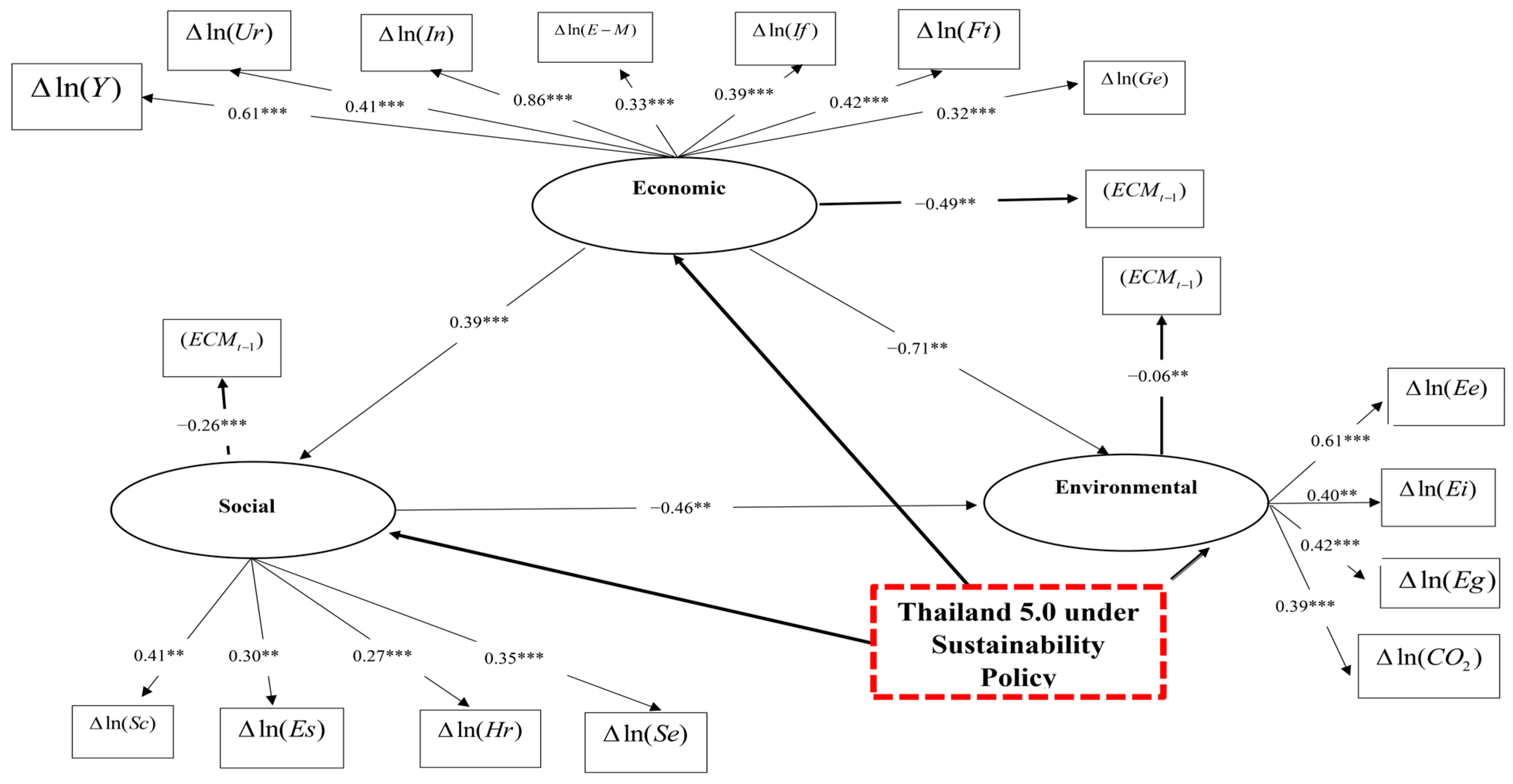
The SEM-VALTM model was developed with three latent variables, economic, social, and environmental, incorporating 15 indicators that are stationary and co-integrated at the same level. This model effectively demonstrates the influence of relationships through the SEM-VALTM model. Detailed results are shown in Figure 3.
From Figure 3, it is evident that the latent variables exhibit both direct and indirect effects. The SEM-VALTM model has been validated with the following criteria: the χ 2 / d f value is 1.55, R M S E A value is 0.01, R M R value is 0.001, G F I value is 0.96, A G F I value is 0.94, R-squared is 0.96, the F-statistic is 225.00 (with a probability of 0.00), the ARCH test is 20.15 (with a probability of 0.1), and the LM test is 1.11 (with a probability of 0.10). Moreover, the SEM-VALTM model has passed the test for Best Linear Unbiased Estimation (BLUE) completely. The analysis reveals that the SEM-VAL model effectively analyzes the relationships and the direction of these relationships between the latent variables: the economic sector and environmental sector show an inverse relationship; the economic sector and social sector show a positive relationship; and the social sector and environmental sector show an inverse relationship. The relationships between the latent variables arise from the observed variables in each sector, which exhibit varying levels of influence, as detailed below:
  • Economic Sector: At a statistical significance level of α = 0.01, the observed variable with the highest influence is the industrial structure rate ( ln I n ) , followed by the per capita GDP rate ( ln Y ) , the foreign tourist rate ( ln F t ) , the urbanization rate ( ln U r ) , the indirect foreign investment rate ( ln I f ) , the total exports rate ( ln E m ) , and the government expenditure rate ( ln G e ) , respectively.
  • Social Sector: At a statistical significance level of α = 0.01, the observed variable with the highest influence is the consumer protection rate ( ln S c ) , followed by the social security rate ( ln S e ) , the employment rate ( ln E s ) , and the health and illness rate ( ln H r ) , respectively.
  • Environmental Sector: At a statistical significance level of α = 0.01, the observed variable with the highest influence is the total energy consumption rate ( ln E e ) , followed by the green technology rate ( ln E g ) , the renewable energy rate ( ln E i ) , and carbon dioxide emissions ( ln C O 2 ) , respectively.
Thus, the SEM-VAL model effectively demonstrates the detailed relationships among causal factors, including both direct and indirect effects. The magnitude of influence is detailed in Table 3.
Based on Table 3, the SEM-VALTM model has successfully passed validity checks, with RMSEA and RMR values approaching 0, indicating good model fit. Additionally, the GFI and AGFI values are close to 1, further confirming model adequacy. The examination of BLUE (Best Linear Unbiased Estimation) did not reveal issues of heteroskedasticity, multicollinearity, or autocorrelation. In terms of model performance, the determination coefficient (R-square) is 97%, indicating that the model explains 97% of the variance in the dependent variables, and the F-test value is 75.05, significant at the 1% level, indicating overall model significance.
The analysis results show that the economic sector has a direct effect on the social sector of 39% in the same direction at the 1% significance level. This implies that a 1% change in the economic sector leads to a 39% change in the social sector in the same direction. The economic sector has a direct effect on the environmental sector of 71% in the opposite direction at the 1% significance level. This indicates that a 1% change in the economic sector results in a 71% change in the environmental sector in the opposite direction. The social sector has a direct effect on the environmental sector of 46% in the opposite direction at the 1% significance level. This shows that a 1% change in the social sector leads to a 46% change in the environmental sector in the opposite direction.
In this research, various findings have emerged from the analysis using the SEM-VALTM model. The research has uncovered insights into the error correction mechanism ( E C M t 1 ) , particularly in the economic sector. The parameter value is −0.49, significant at the 1% level, indicating that adjustments in the economic sector have a 49% capacity to revert to equilibrium. This signifies the highest adjustment speed towards equilibrium. Furthermore, the social sector and environmental sector exhibit lower adjustment capacities towards equilibrium ( E C M t 1 ) , at 26% and 6%, respectively, indicating their relative slower rates of adjustment compared to the economic sector.
From this research, it was discovered that the SEM-VALTM model demonstrates that the industrial structure rate in the economic sector has the most significant negative influence on the environmental sector, resulting in the greatest ecological damage. Furthermore, it was found that the environmental sector has the most difficulty in recovering to its normal state. Therefore, as a proactive strategic approach, the researcher has formulated a new scenario policy emphasizing the use of clean technology and renewable capabilities.
In this research, the researcher employed sensitivity analysis on all factors to examine their suitability for use in formulating the new scenario policy. The results indicated that the factors with statistical significance at a 99% confidence level, ranking highest in both short-term and long-term tests, were clean technology and renewable energy. In the social sector, it was found that only the employment rate passed the sensitivity analysis in the short term. However, in the long term, it did not meet the 99% confidence level requirement. Therefore, the researcher prioritized developing the new scenario policy based on these variables to urgently devise strategies for managing Thailand, particularly to reduce greenhouse gas emissions. If economic and environmental measures are effectively implemented, it is expected that strategies addressing social dimensions can be formulated in subsequent phases. When considering the magnitude of influence between sectors, the economic sector was found to have the greatest impact on the environmental sector, followed by the social sector. This underscores that changes in the economic sector will most significantly affect the environmental sector.
The results suggest that the researcher concludes that the SEM-VALTM model can be used to measure performance for forecasting purposes, ensuring its reliability for future forecasting applications. Additionally, the researcher utilized the data from this study to apply it to various previously established models for comparison of their performance. These models include the Artificial Neural Network (ANN model), Multivariate Adaptive Regression Splines (MARP model), Gradient Boosting (GB model), Gray model, and Autoregressive Integrated Moving Average with Exogenous Variables (ARIMAX model). Performance was evaluated using statistical measures, such as MAPE and RMSE, as presented in the following Table 4:
Table 4 presents the results of performance evaluation for the SEM-VALTM model and previously established models, including the ANN model, MARP model, GB model, Gray model, and ARIMAX model. The researcher utilized secondary data spanning from 1990 to 2024 and incorporated the factors outlined above. To ensure the highest effectiveness in performance measurement, all models were constructed using the same controlled factors. The research findings indicate that the SEM-VALTM model achieved the lowest MAPE and RMSE values compared to the other models, with values of 1.09% and 1.71%, respectively. Therefore, the researcher selected the SEM-VALTM model to forecast greenhouse gas emissions based on current energy consumption. This was used to compare the ecological damage resulting from greenhouse gas emissions under the new scenario policy, which emphasizes clean technology and renewable capabilities, as detailed below.

4.4. Forecasting the Results of Total Energy Consumption and Greenhouse Gas Emissions Using the SEM-VALTM Model

For this forecast, the researcher applied the SEM-VALTM model based on the newly formulated scenario policy to predict total energy consumption. The results of the total energy consumption forecast were then utilized to support the subsequent forecast of greenhouse gas emissions.
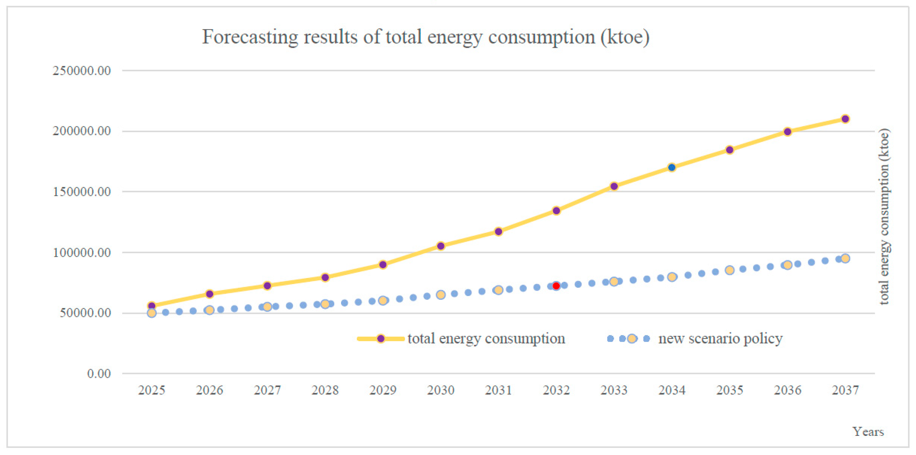
  • The total energy consumption forecast using the SEM-VALTM model for the period 2025 to 2037 is shown in Figure 4.
From Figure 4, it is evident that total energy consumption between 2025 and 2037 shows a dramatic increase. In 2025, energy consumption was recorded at 55,872.90 ktoe, escalating sharply to 210,061.30 ktoe by 2037, with a growth rate (2037/2025) of 275.96%. This rate significantly exceeds the carrying capacity standard of 13,025.50 ktoe. However, when a new scenario policy was implemented within the SEM-VAL model, the energy consumption trend showed a marked reduction in growth. By 2037, the consumption will be limited to 95,027.89 ktoe, with a significantly lower growth rate (2037/2025) of 90.01%. This reduction demonstrates that the adjusted policies help ensure that future energy consumption aligns with sustainability goals. These findings were subsequently utilized to analyze trends in greenhouse gas emissions for the same period (2025 to 2037) to further evaluate the environmental impacts under different scenarios.
2.
Forecasting Results of Greenhouse Gas Emissions Using the SEM-VALTM Model (2025–2037)
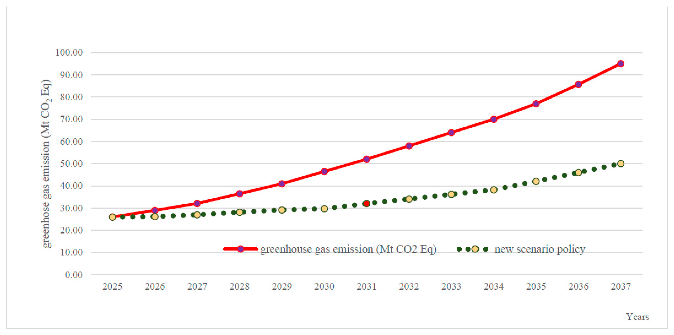
From Figure 5, the forecasted trend in greenhouse gas emissions between 2025 and 2037 reveals a significant rise. In 2025, emissions were recorded at 26.05 Mt CO2 Eq., increasing sharply to 95.05 Mt CO2 Eq. in 2037, with a dramatic growth rate (2037/2025) of 264.88%. This growth rate far exceeds the carrying capacity threshold of 60.5 Mt CO2 Eq., posing a serious risk of ecological damage and surpassing the environment’s ability to recover. According to risk management principles, immediate measures must be taken to mitigate greenhouse gas emissions. This research identified energy consumption in the environmental sector as the most influential factor driving greenhouse gas emissions. Therefore, it is critical for the government to adopt a new scenario policy prioritizing renewable energy sources and clean technology. The analysis further revealed that under the new scenario policy, energy consumption trends will decline significantly, leading to greenhouse gas emissions rising to only 50.04 Mt CO2 Eq. by 2037, with a reduced growth rate (2037/2025) of 92.46%. This revised growth rate falls within the carrying capacity, ensuring sustainability. This finding underscores the importance of integrating the SEM-VAL model, which offers superior accuracy in forecasting compared to historical models, as a foundational tool into national policy formulation. The insights provided by this research represent a valuable framework for guiding sustainable national development and addressing long-term environmental challenges.

5. Discussion

In this qualitative research, the SEM-VALTM model was developed, emerging as the most effective model due to its strong validity and marked improvement over previous models. This model meticulously accounts for both direct and indirect effects, precisely defining the relationships and their magnitudes, thereby avoiding misleading results. The findings align seamlessly with the research hypotheses and exhibit high quality and practical relevance. Additionally, the SEM-VALTM model facilitated new insights from quantitative data, demonstrating that the economic sector exerts the most significant influence on changes in the environmental sector. These changes, driven by economic activities, have a substantial negative impact, escalating environmental degradation. Furthermore, the environmental sector was identified as having the slowest recovery rate, often failing to adapt to balance, which intensifies the damage. The research also highlights the inefficiency of Thailand’s past sustainability policy implementation, calling for the government to adopt innovative governance strategies. These strategies should integrate proactive and reactive measures to stabilize the economic sector and ensure sustainable progress towards Thailand 5.0.
The findings further reveal that the SEM-VALTM model is highly effective in analyzing long-term greenhouse gas emissions (2025–2037) in alignment with designated carrying capacity thresholds. When a new scenario policy was introduced, greenhouse gas emissions in Thailand were significantly reduced, growing only to 55.04 Mt CO2 Eq. during 2025–2037, well below the standard carrying capacity of 60.5 Mt CO2 Eq. The analysis showed full alignment with the research hypotheses: the economic sector has the greatest direct negative impact on the environmental sector, indicating that rapid economic development increases ecological damage. Similarly, the social sector has an indirect negative effect on the environmental sector, and the economic sector also indirectly impacts the environment through its influence on the social sector. These findings highlight the risk of pursuing rapid economic growth under Thailand 5.0 policies, as such efforts could further exacerbate environmental damage. To counteract this, the government must urgently implement new scenario policies emphasizing renewable energy and clean technology. These measures are vital for strategic planning and sustainable national development, ensuring ecological balance. Notably, the SEM-VALTM model demonstrated minimal error in the environmental sector, underscoring the sector’s difficulty in achieving equilibrium. Once disrupted, ecological systems are challenging, if not impossible, to restore.
However, the findings of this research indicate that the changes in exogenous latent variables and endogenous latent variables exhibit both the magnitude of influence and the direction of relationships at a statistical significance level of α = 0.01. These findings align with the hypotheses established in this research, which are as follows: (1) the economic sector influences changes in the environmental sector in an inverse direction; (2) the social sector influences changes in the environmental sector in an inverse direction; and (3) the economic sector influences changes in the social sector in the same direction. Additionally, it was found that the economic sector has an indirect effect on the environmental sector through the social sector.
This research has developed the SEM-VALTM model, which proves to be highly valuable and serves as a critical tool for advancing the sustainable governance of Thailand towards Thailand 5.0, especially in long-term national management. Key findings from this study include:
  • The environmental sector has the slowest adjustment capacity to equilibrium. With its current adjustment speed, it could take thousands of years for the ecosystem to return to its natural state, or it may never recover. Therefore, any shock to the system would severely harm the ecosystem, with cascading negative effects across all sectors.
  • Given that the industrial rate has the most significant negative impact on the environmental sector, strategies for a new scenario policy in the agricultural sector must focus on promoting renewable energy and clean technologies. These strategies should be prioritized by the government as the first step in long-term national policy formulation.
This approach aims to avoid past governance errors, where policies were implemented without emphasizing or supporting key areas in the proper order. Such fragmented management failed to reduce greenhouse gas emissions below the carrying capacity. Moving forward, this issue must be declared a national agenda to ensure effective policy implementation and sustainable outcomes.
As for the recommendations for future research, it should focus on applying this study, particularly the SEM-VALTM model, to the agricultural sector. This can be achieved through a mixed-methods approach, integrating both quantitative and qualitative research, to identify strategies for reducing greenhouse gas emissions. Engaging with stakeholders and policymakers will provide deeper practical insights and enhance the applicability of the research. Additionally, this approach can help address existing weaknesses and further refine the research methodology to ensure greater relevance and impact. The model can also be adapted and applied to other contexts, enabling more informed and appropriate decision-making in various areas.
As for the recommendation, this research presents an efficient model for national governance; however, it should be used in conjunction with proactive measures to ensure Thailand’s genuine and sustainable growth in accordance with the principles of Our Common Future, a cornerstone of sustainable development. Additionally, this research provides critical recommendations for maximizing the benefits of applying the SEM-VALTM model to guide strategic decision-making effectively.
  • Comprehensive reforms of Thailand’s environmental protection laws are essential, as the current legal framework is insufficient for addressing contemporary challenges. Accelerating these reforms would improve enforcement and mitigate environmental degradation. Presently, enforcement measures lack adequacy and fail to comprehensively address criminal, civil, and administrative laws.
  • Establishing clear standards for carrying capacities to manage greenhouse gas emissions across all sectors is a critical requirement for Thailand. Continuous monitoring is necessary, as current assessments of carrying capacity only address short-, medium-, and long-term intervals. This approach risks failing to account for true changes or shocks in emission levels.
  • Urgent governmental action is required to allocate appropriate and modern technology to reduce greenhouse gas emissions effectively. Additionally, policy shifts are needed to hold environmental offenders accountable, transforming victims into proactive defenders of environmental rights to reduce communal environmental harm.
  • While the polluter pays principle is theoretically applied in Thailand, its implementation lacks concrete measures, and proving violations remains challenging. Furthermore, Thailand does not have a dedicated environmental court, relying instead on administrative courts, which reduces the efficiency of legal proceedings. Expediting the establishment of such mechanisms is urgently necessary.
This research focuses on identifying strategies for managing Thailand’s greenhouse gas emissions, emphasizing the urgent adoption of new scenario policies to prevent further environmental damage. Previously, the absence of advanced policy tools and reliance on outdated models often led to spurious results and misdirected national governance strategies. Weak law enforcement and inconsistent implementation exacerbate these challenges, with damage increasing over time. Additionally, the lack of cross-border cooperation on greenhouse gas reduction complicates Thailand’s efforts, as neighboring countries continue to escalate environmental damage.
If Thailand continues on its current trajectory, long-term solutions may become unattainable. Thus, driving the nation’s development towards “Thailand 5.0” requires simultaneous advancements in all sectors, aligning with the policies established during the World Summit (2002). Greater reductions in greenhouse gas emissions will ultimately enhance ecosystems, supporting sustainable and balanced coexistence of humans, animals, and other living organisms.

6. Conclusions

For the SEM-VALTM model in this research, all indicators currently used in Thailand were selected to verify their stationary properties. It was found that 19 indicators could be used in the model as they are stationary at first difference at a 99% confidence interval. When testing for long-term relationships using the co-integration test, it was found that the indicators included in this model exhibited co-integration. This indicates that analyzing long-term relationships is feasible and appropriate. We then analyzed the direct effects and indirect effects using the SEM-VALTM model. The research results revealed that this model is suitable, as it passed the spuriousness test, demonstrating no issues with heteroscedasticity, multicollinearity, or autocorrelation. Additionally, it met the criteria for Best Linear Unbiased Estimation (BLUE) and passed all validity tests for the statistical measures, adhering to all specified standards. Therefore, we conclude that the economic sector has the greatest influence on changes in the environmental sector, with an inverse relationship. Meanwhile, the economic sector also influences changes in the social sector, but in the same direction.
The research findings reveal that the environmental sector has the slowest ability to adjust to equilibrium. If a shock occurs, it will be very difficult, or even impossible, for this sector to return to equilibrium, which is in stark contrast to the economic sector and social sector. Additionally, it was discovered that in the economic sector, the most influential indicator driving changes is industrial structure rate, which has the greatest inverse impact on the environmental sector. To address these challenges, a new scenario policy was proposed, emphasizing the use of clean technology and renewable energy. Based on the research outcomes, the following conclusions were drawn: 1) total energy consumption from 2025 to 2037 is projected to decrease, with a growth rate (2037/2025) rising by only 103.31%, which remains below the carrying capacity; and 2) the analysis of greenhouse gas emissions for the same period (2025–2037) indicates an increase of only 55.04 Mt CO2 Eq., which is at a declining growth rate and remains below the carrying capacity standard of no more than 60.5 Mt CO2 Eq. Thus, the SEM-VALTM model demonstrates comprehensive and appropriate attributes for formulating national management strategies. It serves as a crucial tool for future decision-making, positioning Thailand on the path to achieving Thailand 5.0.

Author Contributions

Conceptualization, P.S. (Pruethsan Sutthichaimethee), P.S. (Phayom Saraphirom) and C.J.; methodology, P.S. (Pruethsan Sutthichaimethee), P.S. (Phayom Saraphirom) and C.J.; software, P.S. (Pruethsan Sutthichaimethee), P.S. (Phayom Saraphirom) and C.J.; validation, P.S. (Pruethsan Sutthichaimethee), P.S. (Phayom Saraphirom) and C.J.; formal analysis, P.S. (Pruethsan Sutthichaimethee), P.S. (Phayom Saraphirom) and C.J.; investigation, P.S. (Pruethsan Sutthichaimethee), P.S. (Phayom Saraphirom) and C.J.; resources, P.S. (Pruethsan Sutthichaimethee), P.S. (Phayom Saraphirom) and C.J.; data curation, P.S. (Pruethsan Sutthichaimethee), P.S. (Phayom Saraphirom) and C.J.; writing—original draft preparation, P.S. (Pruethsan Sutthichaimethee), P.S. (Phayom Saraphirom) and C.J.; writing—review and editing, P.S. (Pruethsan Sutthichaimethee), P.S. (Phayom Saraphirom) and C.J.; visualization, P.S., P.S. and C.J.; supervision, C.J. and P.S. (Phayom Saraphirom); project administration, C.J. and P.S. (Phayom Saraphirom) All authors have read and agreed to the published version of the manuscript.

Funding

This research work was supported by the Research Fund of the Faculty of Engineering, Khon Kaen University under the Research Scholarship for Ph.D. Students project under Contract No. Ph.D-004/2567.

Institutional Review Board Statement

Not applicable.

Informed Consent Statement

Not applicable.

Data Availability Statement

Data are contained within the article.

Acknowledgments

This research work was supported by the Research Fund of the Faculty of Engineering, Khon Kaen University under the Research Scholarship for Ph.D. Students project under Contract No. Ph.D-004/2567. This research was supported by the Postharvest Technology Innovation Center, Science, the Research and Innovation Promotion and Utilization Division, the Office of the Ministry of Higher Education, Science, Research and Innovation, Thailand, and the Agricultural Machinery and Postharvest Technology Center, Khon Kaen University, Thailand.

Conflicts of Interest

The authors declare no conflicts of interest.

References

  1. Office of the National Economic and Social Development Council (NESDC). Available online: http://www.nesdc.go.th/nesdb_en/more_news.php?cid=154&filename=index (accessed on 20 December 2024).
  2. Thailand Greenhouse Gas Management Organization (Public Organization). Available online: https://www.tgo.or.th/2023/index.php/th/ (accessed on 20 December 2024).
  3. The World Bank: Energy Use (Kg of Oil Equivalent Per Capita) Home Page. Available online: https://data.worldbank.org/indicator/EG.USE.PCAP.KG.OE (accessed on 20 December 2024).
  4. Department of Alternative Energy Development and Efficiency. Available online: https://www.dede.go.th/ (accessed on 21 December 2024).
  5. National Statistic Office Ministry of Information and Communication Technology. Available online: https://www.nso.go.th/nsoweb/index?set_lang=en (accessed on 20 December 2024).
  6. Sutthichaimethee, P.; Kubaha, K. The Efficiency of Long-Term Forecasting Model on Final Energy Consumption in Thailand’s Petroleum Industries Sector: Enriching the LT-ARIMAXS Model under a Sustainability Policy. Energies 2018, 11, 2063. [Google Scholar] [CrossRef]
  7. Sutthichaimethee, P.; Chatchorfa, A.; Suyaprom, S. A Forecasting Model for Economic Growth and CO2 Emission Based on Industry 4.0 Political Policy under the Government Power: Adapting a Second-Order Autoregressive-SEM. J. Open Innov. Technol. Mark. Complex 2019, 5, 69. [Google Scholar] [CrossRef]
  8. Sutthichaimethee, P. A Framework on Setting Strategies for Enhancing the Efficiency of State Power use in Thailand’s Pursuit of a Green Economy. Int. J. Energy Econ. Policy 2024, 14, 108–120. [Google Scholar] [CrossRef]
  9. United Nations Framework Convention on Climate Change, UNFCCC, Bonn, Germany. The Paris Agreement: An Early Assessment. Environ. Policy Law 2014, 44, 485–488. [Google Scholar]
  10. United Nations Framework Convention on Climate Change, UNFCCC, Bonn, Germany. Global Progress in Environmental Law. Environ. Policy Law 2016, 46, 23–27. [Google Scholar]
  11. Sutthichaimethee, P. Forecasting Economic, Social and Environmental Growth in the Sanitary and Service Sector Based on Thailand’s Sustainable Development Policy. J. Ecol. Eng. 2018, 19, 205–210. [Google Scholar] [CrossRef]
  12. Thailand Development Research Institute (TDRI), Making Exports for a Low-Carbon Era. Available online: https://thaicarbonlabel.tgo.or.th/tools/files.php?mod=YjNKbllXNXBlbUYwYVc5dVgyUnZkMjVzYjJGaw&type=WDBaSlRFVlQ&files=TkRrPQ (accessed on 20 December 2024).
  13. Pollution Control Department Ministry of Natural Resources and Environment. Navigation of Thai Waterways Act, B.E. 2546. Available online: https://www.pcd.go.th/publication/3559/ (accessed on 20 December 2024).
  14. Pollution Control Department Ministry of Natural Resources and Environment. Principle 4: In Order to Achieve Sustainable Development, Environmental Protection Shall Constitute an Integral Part of the Development Process and Cannot Be Considered in Isolation from It. Available online: https://www.epd.gov.hk/epd/misc/corp-env/epd-eng/annex1.htm (accessed on 20 December 2024).
  15. Sutthichaimethee, P.; Ariyasajjakorn, D. Forecasting Model of GHG Emission in Manufacturing Sectors of Thailand. J. Ecol. Eng. 2017, 18, 18–24. [Google Scholar] [CrossRef]
  16. Sutthichaimethee, P.; Ariyasajjakorn, D. Forecast of Carbon Dioxide Emissions from Energy Consumption in Industry Sectors in Thailand. Environ. Clim. Technol. 2018, 22, 107–117. [Google Scholar] [CrossRef]
  17. Sutthichaimethee, P.; Ariyasajjakorn, D. Forecasting Model on Carrying Capacity for Government’s Controlling Measure under Environmental Law in Thailand: Adapting Non-recursive Autoregression Based on the Var-X Model. Int. J. Energy Econ. Policy 2020, 10, 645–655. [Google Scholar] [CrossRef]
  18. Sutthichaimethee, P.; Kubaha, K. A Relational Analysis Model of the Causal Factors Influencing CO2 in Thailand’s Industrial Sector under a Sustainability Policy Adapting the VARIMAX-ECM Model. Energies 2018, 11, 1704. [Google Scholar] [CrossRef]
  19. Wang, J.; Jiang, C.; Li, M.; Zhang, S.; Zhang, X. Renewable energy, agriculture, and carbon dioxide emissions nexus: Implications for sustainable development in sub-Saharan African countries. Sustain. Environ. Res. 2023, 33, 31. [Google Scholar] [CrossRef]
  20. Kuldasheva, Z.; Salahodjaev, R. Renewable Energy and CO2 Emissions: Evidence from Rapidly Urbanizing Countries. J. Knowl. Econ. 2022, 14, 1077–1090. [Google Scholar] [CrossRef]
  21. Ike, G.N.; Usman, O.; Alola, A.A.; Sarkodie, S.A. Environmental quality effects of income, energy prices and trade: The role of renewable energy consumption in G-7 countries. Sci. Total Environ. 2020, 721, 137813. [Google Scholar] [CrossRef] [PubMed]
  22. Şanlı, D.; Muratoğlu, Y.; Songur, M.; Uğurlu, E. The asymmetric effect of renewable and non-renewable energy on carbon emissions in OECD: New evidence from non-linear panel ARDL model. Front. Environ. Sci. 2023, 11, 1228296. [Google Scholar] [CrossRef]
  23. Riti, J.S.; Song, D.; Shu, Y.; Kamah, M.; Adi Atabani, A. Does renewable energy ensure environmental quality in favour of economic growth? Empirical evidence from China’s renewable development. Qual. Quant. 2018, 52, 2007–2030. [Google Scholar] [CrossRef]
  24. Iqbal, S.; Wang, Y.; Ahmed Shaikh, P.; Maqbool, A.; Hayat, K. Exploring the asymmetric effects of renewable energy production, natural resources, and economic progress on CO2 emissions: Fresh evidence from Pakistan. Environ. Sci. Pollut. Res. 2022, 29, 7067–7078. [Google Scholar] [CrossRef]
  25. Naz, S.; Sultan, R.; Zaman, K.; Mohammed Aldakhil, A.; Nassani, A.A.; Qazi Abro, M.M. Moderating and mediating role of renewable energy consumption, FDI inflows, and economic growth on carbon dioxide emissions: Evidence from robust least square estimator. Environ. Sci. Pollut. Res. 2019, 26, 2806–2819. [Google Scholar] [CrossRef]
  26. Alola, A.A.; Joshua, U. Carbon emission effect of energy transition and globalization: Inference from the low-, lower middle-, upper middle-, and high-income economies. Environ. Sci. Pollut. Res. 2020, 27, 38276–38286. [Google Scholar] [CrossRef]
  27. Shaari, M.S.; Abidin, N.Z.; Abdul Karim, Z. The Impact of Renewable Energy Consumption and Economic Growth on CO2 Emissions: New Evidence using Panel ARDL Study of Selected Countries. Int. J. Energy Econ. Policy 2020, 10, 617–623. [Google Scholar] [CrossRef]
  28. Arshad, A.; Jadoon, A.K.; Sarwar, A.; Javaid, M.F. Towards Asian Countries Sustainable Development: The Nexus between Information and Communication Technology, Energy Consumption and Carbon Dioxide Emission. Bull. Bus. Econ. 2024, 13, 1–8. [Google Scholar] [CrossRef]
  29. Raihan, A.; Tuspekova, A. Toward a sustainable environment: Nexus between economic growth, renewable energy use, forested area, and carbon emissions in Malaysia. Resour. Conserv. Recycl. Adv. 2022, 15, 200096. [Google Scholar] [CrossRef]
  30. Ansah, S.; Xungang, Z.; Wiafe, E.A.; Ntim-Amo, G. Sustainable Economic Development Routes in Sub-Sahara Africa: A Dynamic Long-Run Relationship Analysis Of Fiscal Policy, Energy Consumption And Carbon Dioxide Emissions. J. Adv. Res. Econ. Adm. Sci. 2022, 32, 64–94. [Google Scholar] [CrossRef]
  31. Abdi, A.H. Toward a sustainable development in sub-Saharan Africa: Do economic complexity and renewable energy improve environmental quality? Environ. Sci. Pollut. Res. 2023, 30, 55782–55798. [Google Scholar] [CrossRef] [PubMed]
  32. Pindiriri, C.; Chidoko, C. The Impact Assessment of Sustainable Development Assistance on Carbon Dioxide Emissions: The Sub-Saharan Africa Experience. J. Sustain. Dev. Afr. 2012, 14, 182–198. [Google Scholar]
  33. Adendorff, C.M.; Keown, H.; Amansure, R. The development of a socio-economic model to promote women’s empowerment initiatives in the renewable energy sector of South Africa. J. Energy South. Afr. 2020, 31, 34–47. [Google Scholar] [CrossRef]
  34. You, C.; Khattak, S.I.; Ahmad, M. Do international collaborations in environmental-related technology development in the U.S. pay of in combating carbon dioxide emissions? Role of domestic environmental innovation, renewable energy consumption, and trade openness. Environ. Sci. Pollut. Res. 2022, 29, 19693–19713. [Google Scholar] [CrossRef]
  35. Yu, S.; Chang, C.T.; Ma, C.M. Simulation and measurement of air quality in the traffic congestion area. Sustain. Environ. Res. 2021, 31, 26. [Google Scholar] [CrossRef]
  36. Sooktawee, S.; Kanchanasuta, S.; Bunplod, N. Assessment of 24-h moving average PM2.5 concentrations in Bangkok, Thailand against WHO guidelines. Sustain. Environ. Res. 2023, 33, 3. [Google Scholar] [CrossRef]
  37. Cai, K.; Zhang, X.; Zhang, M.; Ge, Q.; Li, S.; Qiao, B.; Liu, Y. Improving air pollutant prediction in Henan Province, China, by enhancing the concentration prediction accuracy using autocorrelation errors and an Informer deep learning model. Sustain. Environ. Res. 2023, 33, 13. [Google Scholar] [CrossRef]
  38. Rehman, A.; Deyuan, Z. Pakistan’s energy scenario: A forecast of commercial energy consumption and supply from different sources through 2030. Energy Sustain. Soc. 2018, 8, 26. [Google Scholar] [CrossRef]
  39. Almuhtady, A.; Alshwawra, A.; Alfaouri, M.; Al-Kouz, W.; Al-Hinti, I. Investigation of the trends of electricity demands in Jordan and its susceptibility to the ambient air temperature towards sustainable electricity generation. Energy Sustain. Soc. 2019, 9, 39. [Google Scholar] [CrossRef]
  40. Schrammel, J.; Diamond, L.M.; Fröhlich, P.; Mor, G.; Cipriano, J. Influencing residential electricity consumption with tailored messages: Long-term usage patterns and effects on user experience. Energy Sustain. Soc. 2023, 13, 15. [Google Scholar] [CrossRef]
  41. Allen, P.; Hammond, G.P. Bioenergy utilization for a low carbon future in the UK: The evaluation of some alternative scenarios and projections. BMC Energy 2019, 1, 3. [Google Scholar] [CrossRef]
  42. Tilahun, F.B.; Bhandari, R.; Mamo, M. Supply optimization based on society’s cost of electricity and a calibrated demand model for future renewable energy transition in Niger. Energy Sustain. Soc. 2019, 9, 31. [Google Scholar] [CrossRef]
  43. Awafo, E.A.; Akolgo, G.A.; Awaafo, A. Assessment of agricultural residue potential for electrifcation of of-grid communities in the Sawla-Tuna-Kalba District of Ghana. Energy Sustain. Soc. 2024, 14, 50. [Google Scholar] [CrossRef]
  44. Momodu, A.S.; Addo, A.; Kayode Akinbami, J.F.; Mulugetta, Y. Low-carbon development strategy for the West African electricity system: Preliminary assessment using System dynamics approach. Energy Sustain. Soc. 2017, 7, 11. [Google Scholar] [CrossRef]
  45. Zhu, X.; Zhu, J.; Wu, B.; Liu, M.; Wang, G.; Zhu, Z.; Gan, Z.; Zhang, J.; Meng, C. Energy planning for an eco-city based on a distributed energy network. Energ. Sustain. Soc. 2021, 11, 8. [Google Scholar] [CrossRef]
  46. Zhou, C.; Chen, X. Forecasting China’s energy consumption and carbon emission based on multiple decomposition strategy. Energy Strategy Rev. 2023, 49, 101160. [Google Scholar] [CrossRef]
  47. Sahin, U.; Chen, Y. Assessing the current and future effects of Covid-19 on energy related-CO2 emissions in the United States using seasonal fractional grey model. Energy Strategy Rev. 2023, 50, 101234. [Google Scholar] [CrossRef]
  48. Enders, W. Applied Econometrics Time Series; Wiley Series in Probability and Statistics; University of Alabama: Tuscaloosa, AL, USA, 2010. [Google Scholar]
  49. Harvey, A.C. Forecasting, Structural Time Series Models and the Kalman Filter; Cambridge University Press: Cambridge, UK, 1980. [Google Scholar]
  50. Velos, S.P.; Go, M.B.; Bate, G.P.; Joyohoy, E.B. A Seasonal Autoregressive Integrated Moving Average (SARIMA) Model to Forecasting Tourist Arrival in the Philippines: A Case Study in Moalboal, Cebu (Philippines). Recoletos Multidiscip. Res. J. 2020, 8, 67–78. [Google Scholar] [CrossRef]
  51. Dickey, D.A.; Fuller, W.A. Likelihood ratio statistics for autoregressive time series with a unit root. Econometrica 1981, 49, 1057–1072. [Google Scholar] [CrossRef]
  52. MacKinnon, J. Critical Values for Cointegration Test in Long-Run Economic Relationships; Engle, R., Granger, C., Eds.; Oxford University Press: Oxford, UK, 1991. [Google Scholar]
  53. Johansen, S. Likelihood-Based Inference in Cointegrated Vector Autoregressive Models; Oxford University Press: New York, NY, USA, 1995. [Google Scholar]
  54. Johansen, S.; Juselius, K. Maximum likelihood estimation and inference on cointegration with applications to the demand for money. Oxf. Bull. Econ. Stat. 1990, 52, 169–210. [Google Scholar] [CrossRef]
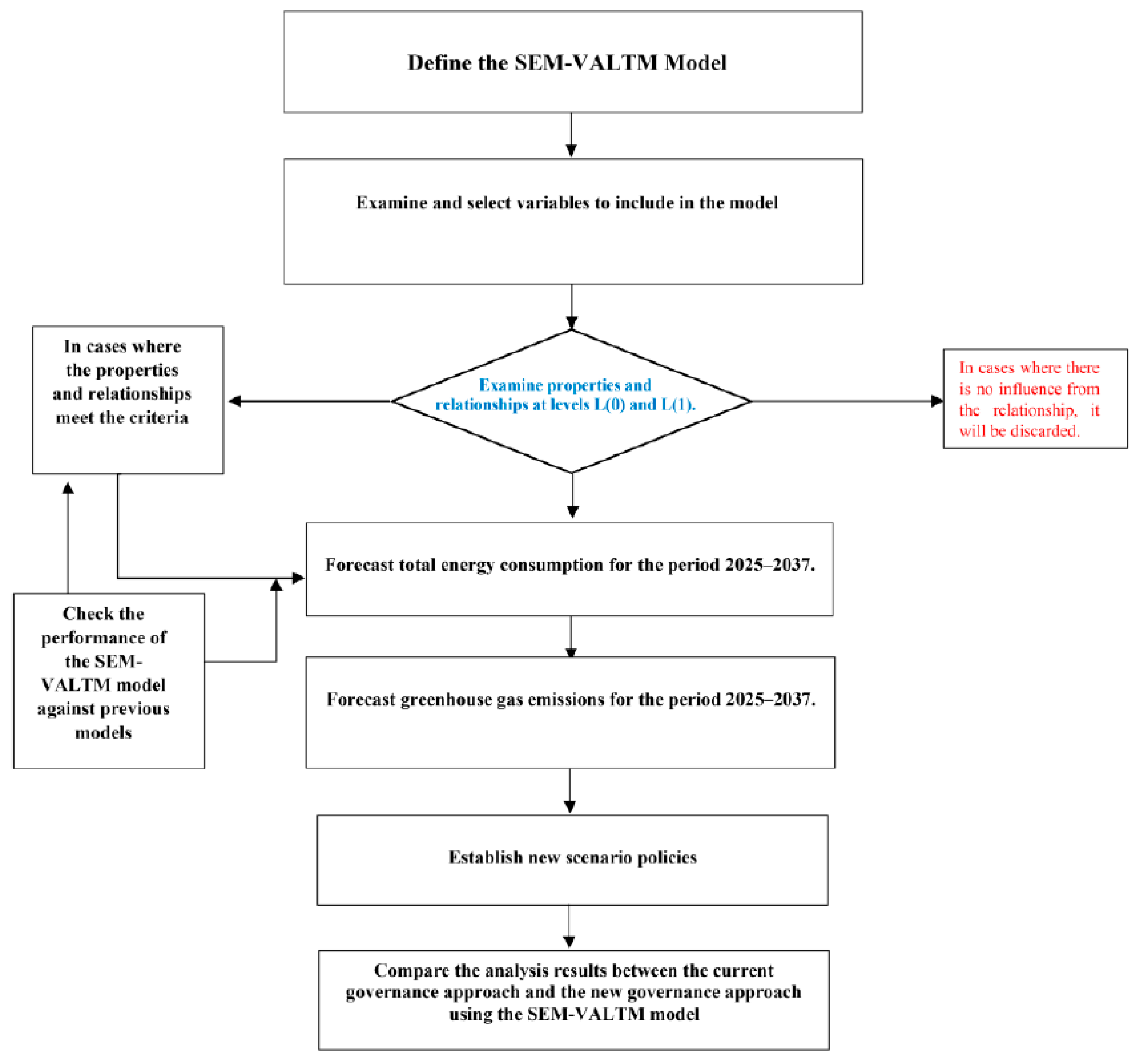
Figure 1. Research Implementation Steps.
Applsci 15 01485 g001
Figure 2. Relationship Characteristics of the SEM-VALTM Model.
Applsci 15 01485 g002
Figure 3. Analysis of Causal Relationships in the SEM-VALTM Model. *** denotes a significance, = 0.01, ** denotes a significance, = 0.05.
Applsci 15 01485 g003
Figure 4. The forecasting results of total energy consumption from 2025 to 2037 in Thailand.
Applsci 15 01485 g004
Figure 5. The forecasting results of greenhouse gas emission from 2025 to 2037 in Thailand.
Applsci 15 01485 g005
Table 1. Unit Root Test at Level I(0) and First Difference I (1).
Tau Test MacKinnon Critical Value
VariablesLevel I(0) ValueVariablesFirst Difference I(1) Value1%5%10%
ln ( Y ) −3.01 Δ ln ( Y ) −4.73 ***−3.85−3.15−2.70
ln ( U r ) −3.11 Δ ln ( U r ) −5.01 ***−3.85−3.15−2.70
ln ( I n ) −3.55 Δ ln ( I n ) −6.40 ***−3.85−3.15−2.70
ln ( E M ) −3.00 Δ ln ( E M ) −4.55 ***−3.85−3.15−2.70
ln ( I f ) −2.75 Δ ln ( I f ) −4.59 ***−3.85−3.15−2.70
ln ( F t ) −2.39 Δ ln ( F t ) −4.60 ***−3.85−3.15−2.70
ln ( G e ) −2.55 Δ ln ( G e ) −4.35 ***−3.85−3.15−2.70
ln ( E s ) −3.05 Δ ln ( E s ) −4.77 ***−3.85−3.15−2.70
ln ( H r ) −3.77 Δ ln ( H r ) −4.79 ***−3.85−3.15−2.70
ln ( S e ) −3.01 Δ ln ( S e ) −4.66 ***−3.85−3.15−2.70
ln ( S c ) −2.50 Δ ln ( S c ) −4.79 ***−3.85−3.15−2.70
ln ( E e ) −3.15 Δ ln ( E e ) −5.05 ***−3.85−3.15−2.70
ln ( E i ) −3.05 Δ ln ( E i ) −5.11 ***−3.85−3.15−2.70
ln ( E g ) −3.79 Δ ln ( E g ) −5.73 ***−3.85−3.15−2.70
ln ( C O 2 ) −3.55 Δ ln ( C O 2 ) −5.09 ***−3.85−3.15−2.70
Note: *** denotes a significance, α = 0.01, Δ is the first difference, and ln is the natural logarithm.
Table 2. Co-integration test by Johansen and Juselius.
VariablesHypothesized No of CE(S)Trace Statistic TestMax-Eigen Statistic TestMacKinnon Critical Value
1%5%
Δ ln ( Y ) , Δ ln ( U r ) , Δ ln ( I n ) , Δ ln ( E M ) , Δ ln ( I f ) , Δ ln ( F t ) , Δ ln ( G e ) , Δ ln ( E s ) , Δ ln ( H r ) , Δ ln ( S e ) , Δ ln ( S c ) , Δ ln ( E e ) , Δ ln ( E i ) , Δ ln ( E g ) , Δ ln ( C O 2 ) None ***255.01 ***201.05 ***15.0510.25
At Most 1 ***85.00 ***81.01 ***11.257.45
*** denotes significance α = 0.01.
Table 3. The results of the relationship size analysis of the SEM-VALTM model.
Dependent VariablesType of EffectIndependent Variables
Economic Social Environmental Error Correction Mechanism ( E C M t 1 )
EconomicDE---−0.49 ***
IE----
SocialDE0.39 ***--−0.26 ***
IE----
EnvironmentalDE0.71 ***0.46 ***-−0.06 ***
IE0.10 ***---
Note: In the above, *** denotes significance, α = 0.01, DE is a direct effect, and IE is an indirect effect.
Table 4. Performance Measurement Results for Forecasting.
Forecasting ModelMAPE (%)RMSE (%)
ANN model15.5517.50
MARP model12.2515.05
GB model9.0510.15
Gray model6.058.95
ARIMAX model6.018.25
SEM-VALTM model1.091.71
Disclaimer/Publisher’s Note: The statements, opinions and data contained in all publications are solely those of the individual author(s) and contributor(s) and not of MDPI and/or the editor(s). MDPI and/or the editor(s) disclaim responsibility for any injury to people or property resulting from any ideas, methods, instructions or products referred to in the content.