
Optimizing Cervical Cancer Diagnosis with Feature Selection and Deep Learning


Abstract
1. Introduction
- Main factors that include age of the patient, chronic inflammation of the HPV virus, early sexual relationship experience, large number of sex partners, large number of child deliveries, long smoking habits, and low economic status.
- Possible factors that include long use of contraceptive pills, a diet rich in antioxidants, HIV infection, as well as frequent, untreated inflammations.
2. Materials and Methods
2.1. Diagnostic Process Overview
- Low-Grade Squamous Intraepithelial Lesion—also called LSIL. This grade describes a non-cancerous lesion in which cells of the uterine cervix are slightly abnormal (see Figure 2b).
- High-Grade Squamous Intraepithelial Lesion—also called HSIL. Describes these cases that can become cancerous. Here, uterine cervix cells are moderately or severely abnormal (see Figure 2c).
2.2. Cervical Cancer Classification
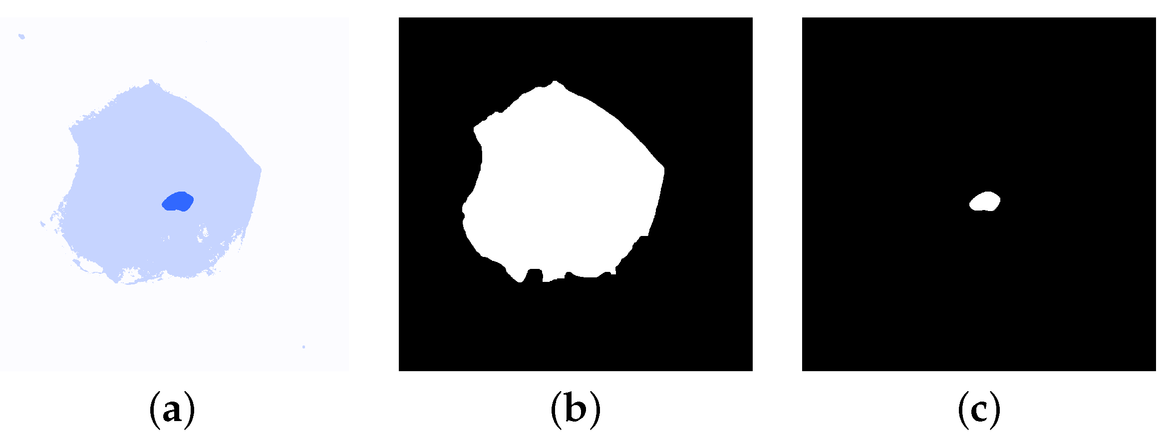
2.3. Image Segmentation
2.4. Feature Extraction
- Nucleus size ()—is defined as the sum of all nuclei pixels in the nucleus.
- Cell size ()—is calculated as the total number of pixels of the cell in the segmented image.
- Nucleus/cell ratio ()—this feature was calculated as a ratio of the nucleus size and the cell size, providing insights into nuclear enlargement, a hallmark of malignancy:
- Nucleus perimeter ()—we define as the length of the nuclear boundary of a nucleus N that is approximated by a length of the polygonal approximation of the boundary [34].
- Cell perimeter ()—similar to , cell diameter is defined as the length of the cell membrane of a cell C that is approximated by the polygonal approximation length of the membrane.
- Nucleus/cell perimeter ratio ()—this feature was calculated as a ratio of nucleus diameter and cell diameter:
- Min Axis ()— is calculated as a shortest Euclidean distance between extreme points of the segmented region both for nucleus and a cell.
- Min Axis ratio ()—represents a ratio between Min Axis for nucleus and a cell
- Max Axis ()— is calculated as a largest Euclidean distance between extreme points of the segmented region both for nucleus and a cell.
- Max Axis ratio ()—determined as a ratio between for the nucleus and a cell.
- Nucleus Aspect Ratio ()—to compute the aspect ratio, the bounding box () of a nucleus is obtained. Feature is calculated as a ratio between width () and height () of the bounding box.
- Cell Aspect Ratio ()—this feature is similar to . Here, the bounding box is determined according to the cell image rather than the nucleus.
- Nucleus/cell Aspect Ratio ()—here, we calculate the ratio of and .
- Extent ()—extent is a feature that represents the amount of space that the nucleus or a cell occupies with respect to its bounding box. We calculate this feature according to Equation (6). It provides information about how compact or irregular a shape is.where represents the size of a nucleus or a cell.
- Nucleus/cell extent ()—is a ratio of nucleus extent and cell extent.
- Solidity ()—solidity measures the smoothness or irregularity of the nucleus boundary. It represents the number of pixels occupied by the object but with respect to its convex hull (). Solidity is defined by Equation (7).where represents the size of a nucleus or a cell and is an area of .
- Nucleus/cell solidity ()—defined as a ratio between and
- Equivalence diameter ()—equivalence diameter is simply a diameter of a circle which area is the same as N or C.
- Equivalence diameter ratio ()—is a ratio between equivalence diameter of the nucleus and the equivalence diameter of a cell.
- Orientation ()—this feature is known as an axis of the least second moment and provides the information about the angle between the row axis when the coordinate system is placed and the centroid of the nucleus/cell. We calculate the orientation according to Equation (8) [35].where the angle is measured counterclockwise from the x–axis.
- Orientation ratio ()—similar to the previous features, it is defined as a ratio between the nucleus and cell orientations.

| Feature | NSIL | LSIL | HSIL |
|---|---|---|---|
| Nucleus size | Very small | Smaller than of cell size | Larger than of cell size |
| Cell size | Large cell | Modest decrease | Significant decrease |
| Nucleus/cell ratio | 1:10 | Change in favor of nucleus | Significant change in favor of nucleus |
| Stainability | Normal | Hyper-stainability | Hyper-or-hypo-stainability |
| Brightness around nucleus | None | Can be visible | None |
2.5. Feature Selection and Ranking
- Kruskal–Wallis TestThis is a non-parametric statistical test used to rank features based on their discriminatory power across diagnostic categories. It determines if the samples originate from the same distribution [37]. It is often regarded as the one-way ANOVA method on ranks or groups. The null hypothesis assumes that the cumulative distribution functions in the populations are equal, for . For this test, we recorded a probability value (p-value) for the null hypothesis.
- Kormogolov–Smirnov TestThis statistical metric represents characteristics through a distribution associated with a data sample [38,39]. This test determines whether the samples are drawn from the same distribution. If the samples come from two different distributions, then the KS test returns a value 1, otherwise it returns a value 0.
- Friedman TestA test proposed by Milton Friedman [40] that can be used for feature ranking. It assesses differences between at least three correlated classes. Here, we recorded a probability value (p-value) for this nonparametric Friedman test.
- Stepwise Feature SelectionThis is an iterative approach that adds or removes features to maximize classification performance. Given a set of extracted features, the stepwise feature selection method (SFS) chooses a subset of features that provide the best performance. The method performs a forward feature selection that in an iterative way adds the best features to the subset of selected features. In every iteration, the best prediction features are used and their significance is estimated with the F-test (see [41]). Here, we use the backward version of this algorithm (SBS), where the assumption is made that initially all features of the original feature set are used. At each iteration, the features with the worst prediction are eliminated.
- Significant Feature SelectionThis retains features with statistically significant differences between classes. Significant feature selection (SBS) uses statistical significance to reduce the full vector of features. This method estimates a for each feature in the feature vector. This calculation is based on the two-sample Student’s t-test for the difference of the population means with unequal variances with the assumption that samples are normally distributed. Usually, we consider a feature being statistically significant if its is smaller than 0.05 which is a typical significance value in biomedical sciences and elsewhere.
2.6. Feature Classification
- Linear discriminant analysis—here, we define a function that is a linear combination of the observations x (see Equation (9)):where w is the weighting vector and is a bias [42]. If , then Equation (9) defines a decision surface and separates observations of one class from another class. For a two-category classifier, we classify the data into first class () if and second class () if . For , the observation is classified into either class.For a multi-class problem we need to define several linear discriminant functions as in Equation (9). The number of functions should be the same as the number of classes used for classification. In this case, a classification rule will be defined by Equation (10).where is the number of classes. Equation (10) defines the decision regions for classes where is the largest discriminant for in that region.
- K-Nearest Neighbors (KNN)—a popular and simple classifier that classifies a new data point based on the majority class among its k closest neighbors in the feature space [42]. Training of the KNN classifier consists of saving a feature vector values along with class label. The classification is based on the calculation of the distance metric, typically the Euclidean distance, to find the k closest points [43]. In this work, we also adopted the same metric, but additionally we have tested different numbers (between 1 and 10) of neighbors taken for label estimation. In the result section (see Section 4) we showed accuracy values for and .
- Support Vector Machines (SVM)—used to separate two or more classes of observations by constructing a boundary between them using border points from each class called support vectors [44]. Here, we employ a kernel-based approach to segregate data, which ensures a robust generalization of the problem. In this way, the classification of an unknown point is classified by its position with respect to the boundary. Training of the SVM model involves an iterative minimization of an error function (Equation (11)).with the following restrictions:where C and b are constants, w is the weight vector, is a bias value that deals with overlapping cases and is a kernel function that transforms input data into the feature space. The constant C has a significant influence on the error rate and must be carefully estimated during the training process. In this study, we perform a grid search on values varied between and .
- Neural Networks (NN)—designed to simulate the behavior of the human brain to enable computers to learn from data. They consist of multiple layers of interconnected neurons, each connected through connections similar to synapses that carry weighted information. These weights are adjusted during training. The network prediction ability is then optimized based on input features. In this work, we adjust the internal parameters (weights and biases) based on the differences between the actual output and the desired output. This process, known as backpropagation, uses gradient descent to minimize network error across 200 iterations. For optimization, Adam’s optimizer was used and the rectified linear unit (ReLu) was used as an activation function in hidden layers. Here, the learning rate, number of hidden layers, and the number of neurons per layer were fine-tuned, with the learning rate ranging from 0.001 to 0.1 and the number of neurons per layer ranging from 10 to 100.
2.7. Classification Metrics
3. Cervical Cancer Database
- Specimen Collection—the samples were collected with a brush and suspended in a preservation solution.
- Specimen processing—the solution was then processed through an automated separator to isolate cells from debris and placed on glass slides.
- Slide staining—slides were stained using the Papanicolaou technique, which employs specific staining agents to highlight cellular details for morphological analysis. In general, staining methods like hematoxylin and eosin or Papanicolaou staining enhance the visibility of cells and nucleus structures.
- Slide digitization—the stained slides were acquired from the Department of Patomorphology of the Pomeranian Medical University in Szczecin, Poland, and digitized in the Department of Pathology and Oncological Cytology at the Medical University of Wrocław, Poland, using an Olympus BX 51 microscope equipped with an Olympus DP72 camera attached to the microscope head. The images were captured using the Olympus CellD software at a resolution of 300 dpi, with dimensions of 2510 × 1540 pixels. The collected database contains 263 LBC cytology images, with 158 classified as Normal Squamous Intraepithelial Lesion, 70 as High Squamous Intraepithelial Lesion, and 35 as Low Squamous Intraepithelial Lesion. For cell shape analysis, we utilized ImageJ software to extract single cell images, resulting in 428 images: 233 NSIL, 110 HSIL and 85 LSIL, all annotated at the per-cell level. For data curation, the following inclusion and exclusion criteria were applied:
- –
- Inclusion criteria: Slides of adequate quality and clear diagnostic classification by expert pathologists
- –
- Exclusion criteria: Low slides quality, ambiguous diagnoses, or insufficient cellular material for accurate segmentation.
The images were retrospectively collected at a single institution to ensure consistency in sample preparation and diagnostic annotations. Although this limits the diversity of the data set, it provides a high-quality foundation for per-cell classification, which is not available in most public data sets. - Case validation—in the next step, an expert pathomorphologist examined the slides to categorize the samples into NSIL, LSIL, or HSIL based on the Bethesda system criteria. This step provided ground-truth labels for training and validating the classification algorithms.
4. Results
4.1. Feature Vector Reduction Results
4.2. Classification Results
5. Discussion and Conclusions
Author Contributions
Funding
Institutional Review Board Statement
Informed Consent Statement
Data Availability Statement
Conflicts of Interest
Abbreviations
| ANOVA | Analysis of Variance |
| C | Cell Size |
| CH | Convex Hull |
| CNN | Convolutional Neural Network |
| Cp | Cell Perimeter |
| Eq | Equivalence Diameter |
| F-Test | Fisher Test |
| Fr | Friedman Test |
| GLCM | Gray-Level Co-Occurrence Matrix |
| HPV | Human Papillomavirus |
| HSIL | High-Grade Squamous Intraepithelial Lesion |
| k-NN | k-Nearest Neighbors |
| KS Test | Kolmogorov–Smirnov Test |
| LBP | Local Binary Patterns |
| LBC | Liquid-Based Cytology |
| LSIL | Low-Grade Squamous Intraepithelial Lesion |
| MaxA | Maximum Area of a Cell |
| MaxAr | Maximum Aspect Ratio |
| MinA | Minimum Area of a Cell |
| MinAr | Minimum Aspect Ratio |
| N | Nucleus Size |
| Nar | Nucleus Aspect Ratio |
| NCAr | Nucleus-to-Cell Aspect Ratio |
| NCp | Nucleus-to-Cell Perimeter Ratio |
| NCEq | Nucleus-to-Cell Equivalence Diameter Ratio |
| NCExt | Nucleus-to-Cell Extent Ratio |
| NCr | Nucleus-to-Cell Ratio |
| NCOr | Nucleus-to-Cell Orientation Ratio |
| NCs | Nucleus-to-Cell Solidity |
| Np | Nucleus Perimeter |
| NSIL | Normal Squamous Intraepithelial Lesion |
| Or | Orientation of a Cell |
| RGB | Red, Green, Blue |
| ReLU | Rectified Linear Unit |
| SBS | Stepwise Backward Selection |
| SFS | Stepwise Feature Selection |
| Sol | Solidity |
| SVM | Support Vector Machine |
| TBS | The Bethesda System |
References
- Wild, C.P.; Weiderpass, E.; Stewart, B.W. (Eds.) World Cancer Report: Cancer Research for Cancer Prevention; IARC: Lyon, France, 2020. [Google Scholar]
- National Cancer Registry of Poland. Incidence Statistics for 2021. 2021. Available online: https://onkologia.org.pl/en (accessed on 19 November 2024).
- Jeleń, Ł.; Krzyżak, A.; Fevens, T.; Jeleń, M. Influence of Feature Set Reduction on Breast Cancer Malignancy Classification of Fine Needle Aspiration Biopsies. Comput. Biol. Med. 2016, 79, 80–91. [Google Scholar] [CrossRef]
- Stankiewicz, I. Using a Computer Program to Evaluate Cytological Smears Received from the Vaginal Part of the Cervix Using the LBC Method. Master’s thesis, Wroclaw Medical University, Wroclaw, Poland, 2018. [Google Scholar]
- Anurag, A.; Das, R.; Jha, G.K.; Thepade, S.D.; Dsouza, N.; Singh, C. Feature Blending Approach for Efficient Categorization of Histopathological Images for Cancer Detection. In Proceedings of the 2021 IEEE Pune Section International Conference (PuneCon), Pune, India, 16–19 December 2021; pp. 1–6. [Google Scholar]
- Daoud, M.I.; Abdel-Rahman, S.; Bdair, T.M.; Al-Najjar, M.; Al-Hawari, F.; Alazrai, R. Breast Tumor Classification in Ultrasound Images Using Combined Deep and Handcrafted Features. Sensors 2020, 20, 6838. [Google Scholar] [CrossRef] [PubMed]
- Kitchener, H.; Almonte, M.; Thomson, C.; Wheeler, P.; Sargent, A.; Stoykova, B.; Gilham, B.; Baysson, H.; Roberts, C.; Dowie, R.; et al. HPV testing in combination with liquid-based cytology in primary cervical screening (ARTISTIC): A randomised controlled trial. Lancet Oncol. 2009, 10, 672–682. [Google Scholar] [CrossRef]
- Papanicolaou, G.N.; Traut, H.F. The diagnostic value of vaginal smears in carcinoma of the uterus. Am. J. Obstet. Gynecol. 1941, 42, 193–206. [Google Scholar] [CrossRef]
- Papanicolaou, G.N. A new procedure for staining vaginal smears. Science 1942, 95, 438–439. [Google Scholar] [CrossRef]
- Solomon, D.; Kurman, R. The Bethesda System for Reporting Cervical/Vaginal Cytologic Diagnoses: Definitions, Criteria, and Explanatory Notes for Terminology and Specimen Adequacy; Springer: Berlin/Heidelberg, Germany, 2012. [Google Scholar]
- Rahmadwati; Naghdy, G.; Ros, M.; Todd, C.; Norahmawati, E. Cervical Cancer Classification Using Gabor Filters. In Proceedings of the 2011 IEEE First International Conference on Healthcare Informatics, Imaging and Systems Biology, San Jose, CA, USA, 26–29 July 2011; IEEE: Piscataway, NJ, USA, 2011; pp. 48–52. [Google Scholar]
- Mariarputham, E.J.; Stephen, A. Nominated Texture Based Cervical Cancer Classification. Comput. Math. Methods Med. 2015, 2015, 586928. [Google Scholar] [CrossRef] [PubMed]
- Amole, A.; Osalusi, B.S. Textural Analysis of Pap Smears Images for k-NN and SVM Based Cervical Cancer Classification System. Adv. Sci. Technol. Eng. Syst. J. 2018, 3, 218–223. [Google Scholar] [CrossRef]
- Qu, H.; Yan, Z.; Wu, W.; Chen, F.; Ma, C.; Chen, Y.; Wang, J.; Lu, X. Rapid diagnosis and classification of cervical lesions by serum infrared spectroscopy combined with machine learning. In Proceedings of the AOPC 2021: Biomedical Optics, Beijing, China, 20–22 June 2021; Wei, X., Liu, L., Eds.; International Society for Optics and Photonics, SPIE: Beijing, China, 2021; Volume 12067, p. 120670A. [Google Scholar]
- Rajeev, M.A. A Framework for Detecting Cervical Cancer Based on UD-MHDC Segmentation and MBD-RCNN Classification Techniques. In Proceedings of the 2021 2nd Global Conference for Advancement in Technology, Bangalore, India, 1–3 October 2021; pp. 1–9. [Google Scholar]
- Khoulqi, I.; Idrissi, N. Deep learning-based Cervical Cancer Classification. In Proceedings of the 2022 International Conference on Technology Innovations for Healthcare (ICTIH), Magdeburg, Germany, 14–16 September 2022; IEEE: Piscataway, NJ, USA, 2022; pp. 30–33. [Google Scholar]
- Hemalatha, K.; Vetriselvi, V. Deep Learning based Classification of Cervical Cancer using Transfer Learning. In Proceedings of the 2022 International Conference on Electronic Systems and Intelligent Computing, Odisha, India, 17–18 December 2022; pp. 134–139. [Google Scholar]
- Subarna, T.; Sukumar, P. Detection and classification of cervical cancer images using CEENET deep learning approach. J. Intell. Fuzzy Syst. 2022, 43, 3695–3707. [Google Scholar] [CrossRef]
- Hattori, M.; Kobayashi, T.; Nishimura, Y.; Machida, D.; Toyonaga, M.; Tsunoda, S.; Ohbu, M. Comparative image analysis of conventional and thin-layer preparations in endometrial cytology. Diagn. Cytopathol. 2013, 41, 527–532. [Google Scholar] [CrossRef]
- Klug, S.; Neis, K.; Harlfinger, W.; Malter, A.; König, J.; Spieth, S.; Brinkmann-Smetanay, F.; Kommoss, F.; Weyer, V.; Ikenberg, H. A randomized trial comparing conventional cytology to liquid–based cytology and computer assistance. Int. J. Cancer 2013, 132, 2849–2857. [Google Scholar] [CrossRef] [PubMed]
- Sornapudi, S.; Brown, G.; Xue, Z.; Long, R.; Allen, L.; Antani, S. Comparing Deep Learning Models for Multi-cell Classification in Liquid-based Cervical Cytology Images. AMIA Annu. Symp. Proc. 2020, 2019, 820–827. [Google Scholar] [PubMed]
- Hut, I.; Jeftic, B.; Dragicevic, A.; Matija, L.; Koruga, D. Computer-Aided Diagnostic System for Whole Slide Imaging of Liquid-Based Cervical Cytology Sample Classification Using Convolutional Neural Networks. Contemp. Mater. 2022, 13, 169–177. [Google Scholar] [CrossRef]
- Kanavati, F.; Hirose, N.; Ishii, T.; Fukuda, A.; Ichihara, S.; Tsuneki, M. A Deep Learning Model for Cervical Cancer Screening on Liquid-Based Cytology Specimens in Whole Slide Images. Cancers 2022, 14, 1159. [Google Scholar] [CrossRef]
- Wong, L.; Ccopa, A.; Diaz, E.; Valcarcel, S.; Mauricio, D.; Villoslada, V. Deep Learning and Transfer Learning Methods to Effectively Diagnose Cervical Cancer from Liquid-Based Cytology Pap Smear Images. Int. J. Online Biomed. Eng. 2023, 19, 77–93. [Google Scholar] [CrossRef]
- Tan, S.L.; Selvachandran, G.; Ding, W.; Paramesran, R.; Kotecha, K. Cervical Cancer Classification From Pap Smear Images Using Deep Convolutional Neural Network Models. Interdiscip. Sci. Comput. Life Sci. 2024, 16, 16–38. [Google Scholar] [CrossRef] [PubMed]
- Abinaya, K.; Sivakumar, B. A Deep Learning-Based Approach for Cervical Cancer Classification Using 3D CNN and Vision Transformer. J. Imaging Inform. Med. 2024, 37, 280–296. [Google Scholar] [CrossRef]
- Su, Z.; Pietikäinen, M.; Liu, L. From Local Binary Patterns to Pixel Difference Networks for Efficient Visual Representation Learning. In Proceedings of the Image Analysis; Gade, R., Felsberg, M., Kämäräinen, J.K., Eds.; Springer: Cham, Switzerland, 2023; pp. 138–155. [Google Scholar]
- Tarawneh, A.S.; Celik, C.; Hassanat, A.B.; Chetverikov, D. Detailed Investigation of Deep Features with Sparse Representation and Dimensionality Reduction in CBIR: A Comparative Study. Intell. Data Anal. 2018, 24, 47–68. [Google Scholar] [CrossRef]
- Shi, Z.; Liu, X.; Li, Q.; He, Q.; Shi, Z. Extracting discriminative features for CBIR. Multimed. Tools Appl. 2011, 61, 263–279. [Google Scholar] [CrossRef]
- Zhang, J.; Liu, Y. Cervical Cancer Detection Using SVM Based Feature Screening. In Proceedings of the Medical Image Computing and Computer-Assisted Intervention, Malo, France, 26–29 September 2004; Springer: Berlin/Heidelberg, Germany, 2004; pp. 873–880. [Google Scholar]
- Jeleń, Ł.; Krzyżak, A.; Fevens, T.; Jeleń, M. Influence of Pattern Recognition Techniques on Breast Cytology Grading. Sci. Bull. Wroc. Sch. Appl. Inform. 2012, 2, 16–23. [Google Scholar]
- Kowal, M.; Filipczuk, P.; Obuchowicz, A.; Korbicz, J.; Monczak, R. Computer-aided diagnosis of breast cancer based on fine needle biopsy microscopic images. Comput. Biol. Med. 2013, 43, 1563–1572. [Google Scholar] [CrossRef]
- Kanungo, T.; Mount, D.; Netanyahu, N.; Piatko, C.; Silverman, R.; Wu, A. An efficient k–means clustering algorithm: Analysis and implementation. IEEE Trans. Pattern Anal. Mach. Intell. 2002, 24, 881–892. [Google Scholar] [CrossRef]
- Street, N. Xcyt: A System for Remote Cytological Diagnosis and Prognosis of Breast Cancer. In Artificial Intelligence Techniques in Breast Cancer Diagnosis and Prognosis; Jain, L., Ed.; World Scientific Publishing Company: Singapore, 2000; pp. 297–322. [Google Scholar]
- Umbaugh, S. Digital Image Processing and Analysis. Human and Computer Vision Applications with CVIPTools, 2nd ed.; CRC Press: New York, NY, USA, 2011. [Google Scholar]
- Guyon, I.; Elisseeff, A. An Introduction to Variable and Feature Selection. J. Mach. Learn. Res. 2003, 3, 1157–1182. [Google Scholar]
- Kruskal, W.H.; Wallis, W.A. Use of Ranks in One-Criterion Variance Analysis. J. Am. Stat. Assoc. 1952, 47, 583–621. [Google Scholar] [CrossRef]
- Conover, W. Practical Nonparametric Statistics; Wiley: New York, NY, USA, 1980. [Google Scholar]
- Corder, G.W.; Foreman, D.I. Nonparametric Statistics: A Step by Step Approach, 2nd ed.; Wiley: New York, NY, USA, 2014. [Google Scholar]
- Friedman, M. The Use of Ranks to Avoid the Assumption of Normality Implicit in the Analysis of Variance. J. Am. Stat. Assoc. 1937, 32, 675–701. [Google Scholar] [CrossRef]
- Kleinbaum, D.G.; Kupper, L.L.; Nizam, A.; Muller, K.E. Applied Regression Analysis and Multivariable Methods, 4th ed.; Duxbury Press: Belmont, CA, USA, 2007. [Google Scholar]
- Duda, R.; Hart, P.; Stork, D. Pattern Classification, 2nd ed.; Wiley Interscience Publishers: New York, NY, USA, 2000. [Google Scholar]
- Altman, N.S. An introduction to kernel and nearest-neighbor nonparametric regression. Am. Stat. 1992, 46, 175–185. [Google Scholar] [CrossRef]
- Cristianini, N.; Shawe-Taylor, J. An Introduction to Support Vector Machines and Other Kernel-Based Learning Methods; Cambridge University Press: Cambridge, UK, 2000. [Google Scholar]
- Idlahcen, F.; Colere Mboukou, P.F.; Zerouaoui, H.; Idri, A. Whole-slide Classification of H&E-stained Cervix Uteri Tissue using Deep Neural Networks. In Proceedings of the 14th International Joint Conference on Knowledge Discovery, Knowledge Engineering, and Knowledge Management, Valletta, Malta, 24–26 October 2022; pp. 322–329. [Google Scholar] [CrossRef]
- Mohammed, B.A.; Senan, E.M.; Al-Mekhlafi, Z.G.; Alazmi, M.; Alayba, A.M.; Alanazi, A.A.; Alreshidi, A.; Alshahrani, M. Hybrid Techniques for Diagnosis with WSIs for Early Detection of Cervical Cancer Based on Fusion Features. Appl. Sci. 2022, 12, 8836. [Google Scholar] [CrossRef]
- Tharwat, A. Classification Assessment Methods. Appl. Comput. Inform. 2021, 17, 168–192. [Google Scholar] [CrossRef]
- Shaikh, S. Measures Derived from a 2 × 2 Table for an Accuracy of a Diagnostic Test. J. Biom. Biostat. 2011, 2, 1–4. [Google Scholar] [CrossRef]
- Das, N.; Mandal, B.; Santosh, K.; Shen, L.; Chakraborty, S. Cervical cancerous cell classification: Opposition-based harmony search for deep feature selection. Int. J. Mach. Learn. Cybern. 2023, 14, 3911–3922. [Google Scholar] [CrossRef]


| Test | Chosen Features | Reduction Rate |
|---|---|---|
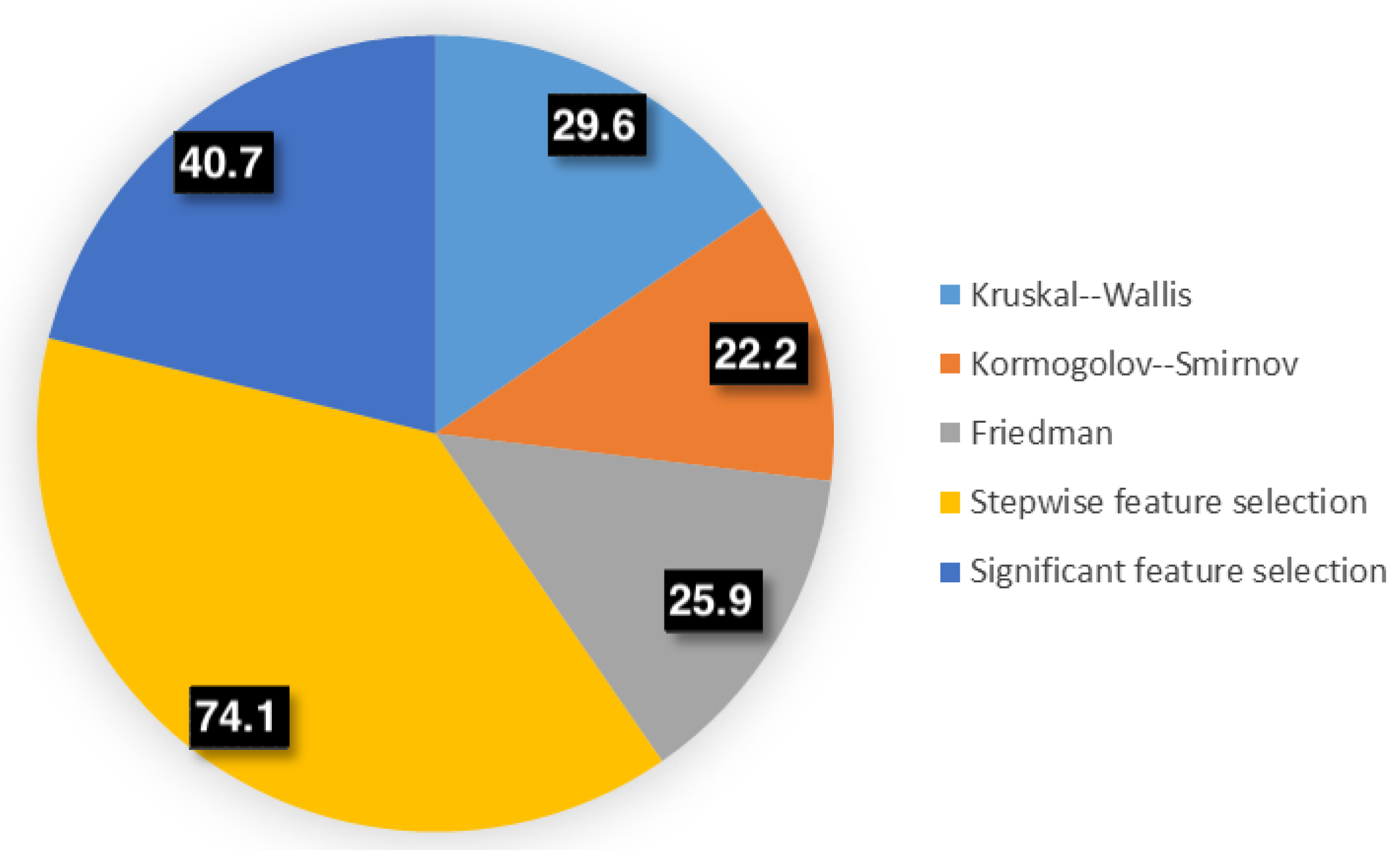
| Kruskal–Wallis | N, C, NCr, Np, Cp, NCp, NMinA, CMinA, NCMinAr, NMaxA, CMaxA, NCMaxr, NExt, NSol, CSol, NCSol, Neq, Ceq, NCeq | 29.6% |
| Kormogolov–Smirnov | N, C, NCr, Np, Cp, NCp, NMinA, CMinA, NCMinAr, NMaxA, CMaxA, NCMaxr, NExt, CExt, NCExt, NSol, CSol, NCSol, Neq, Ceq, NCeq | 22.2% |
| Friedman | N, C, NCr, Np, Cp, NCp, NMinA, CMinA, NCMinAr, NMaxA, CMaxA, NCMaxr, NExt, NCExt, NSol, CSol, NCSol, Neq, Ceq, NCeq | 25.9% |
| Stepwise feature selection | N, C, NCMinAr, CMaxA, NExt, Neq, Ceq | 74.1% |
| Significant feature selection | NCr, Cp, NCp, NMinA, CMinA, NCMinAr, NMaxA, CMaxA, NCMaxr, CAr, NCExt, NSol, NCSol, Neq, Ceq, NCeq | 40.7% |
| CNN | Baseline | KW | KS | Fr | SFS | SBS | |
|---|---|---|---|---|---|---|---|
| NN | 92.9% | 82.7% | 87.7% | 86.3% | 88.1% | 89.7% | 88.1% |
| SVM | 93.3% | 90.1% | 90.9% | 91.8% | 91.4% | 90.1% | 93.0% |
| KNN1 | 87.1 % | 80.7% | 88.9% | 88.5% | 88.9% | 86.8% | 85.6% |
| KNN10 | 84.4 % | 84.0% | 88.5% | 87.7% | 88.1% | 86.8 % | 86.8% |
| Disc. An. | 90.9% | 87.2% | 86.4% | 87.2% | 87.7% | 87.2% | 87.7% |
| Precision (95% CI) | Recall (95% CI) | |||||||||
|---|---|---|---|---|---|---|---|---|---|---|
| NN | SVM | KNN1 | KNN10 | Disc An. | NN | SVM | KNN1 | KNN10 | Disc An. | |
| Baseline | 82.7 (81.5–84.0) | 89.3 (88.0–91.5) | 81.1 (80.0–82.5) | 85.4 (84.0–86.7) | 85.5 (84.1–86.9) | 82.7 (81.5–83.9) | 89.6 (88.5–91.4) | 81.1 (80.0–82.3) | 83.9 (83.0–85.0) | 84.8 (83.2–85.9) |
| KW | 87.6 (85.3–89.7) | 90.9 (89.2–92.7) | 87.5 (85.0–89.8) | 88.5 (86.0–90.8) | 86.6 (85.0–88.1) | 87.7 (85.3–89.9) | 90.9 (89.0–92.9) | 87.2 (84.5–89.6) | 88.5 (86.2–90.4) | 86.4 (84.2–88.0) |
| KS | 86.3 (83.7–88.5) | 88.5 (86.4–90.3) | 86.7 (84.2–88.9) | 89.7 (87.5–91.6) | 87.3 (85.0–89.3) | 86.4 (84.0–88.6) | 88.5 (86.5–90.6) | 86.8 (84.3–88.8) | 89.3 (87.2–91.0) | 86.8 (84.3–88.7) |
| Fr | 88.2 (85.5–90.4) | 89.7 (87.6–91.5) | 85.5 (82.5–88.1) | 90.1 (87.7–92.0) | 87.9 (85.2–90.1) | 88.1 (85.3–90.3) | 89.7 (87.4–91.8) | 85.6 (82.8–87.9) | 89.7 (87.2–91.7) | 87.6 (84.8–90.0) |
| SFS | 89.8 (87.3–92.1) | 88.8 (86.2–91.0) | 88.9 (86.3–91.1) | 87.0 (84.4–89.2) | 86.9 (84.3–89.0) | 89.7 (87.0–92.0) | 88.8 (86.0–91.2) | 88.8 (86.0–91.2) | 86.8 (84.0–89.3) | 86.8 (84.0–89.0) |
| SBS | 88.0 (85.2–90.4) | 91.4 (89.2–93.2) | 84.9 (82.0–87.6) | 89.7 (87.4–91.9) | 85.2 (82.5–87.7) | 88.1 (85.2–90.6) | 91.4 (89.1–93.4) | 85.2 (82.3–87.8) | 89.3 (87.0–91.6) | 84.8 (82.1–87.2) |
Disclaimer/Publisher’s Note: The statements, opinions and data contained in all publications are solely those of the individual author(s) and contributor(s) and not of MDPI and/or the editor(s). MDPI and/or the editor(s) disclaim responsibility for any injury to people or property resulting from any ideas, methods, instructions or products referred to in the content. |
© 2025 by the authors. Licensee MDPI, Basel, Switzerland. This article is an open access article distributed under the terms and conditions of the Creative Commons Attribution (CC BY) license (https://creativecommons.org/licenses/by/4.0/).
Share and Cite
Jeleń, Ł.; Stankiewicz-Antosz, I.; Chosia, M.; Jeleń, M. Optimizing Cervical Cancer Diagnosis with Feature Selection and Deep Learning. Appl. Sci. 2025, 15, 1458. https://doi.org/10.3390/app15031458
Jeleń Ł, Stankiewicz-Antosz I, Chosia M, Jeleń M. Optimizing Cervical Cancer Diagnosis with Feature Selection and Deep Learning. Applied Sciences. 2025; 15(3):1458. https://doi.org/10.3390/app15031458
Chicago/Turabian StyleJeleń, Łukasz, Izabela Stankiewicz-Antosz, Maria Chosia, and Michał Jeleń. 2025. "Optimizing Cervical Cancer Diagnosis with Feature Selection and Deep Learning" Applied Sciences 15, no. 3: 1458. https://doi.org/10.3390/app15031458
APA StyleJeleń, Ł., Stankiewicz-Antosz, I., Chosia, M., & Jeleń, M. (2025). Optimizing Cervical Cancer Diagnosis with Feature Selection and Deep Learning. Applied Sciences, 15(3), 1458. https://doi.org/10.3390/app15031458