Parameter Study and Engineering Verification of the Hardening Soil Model with Small-Strain Stiffness for Loess in the Xi’an Area

Abstract

With the advancement of the construction of urban underground spaces, it is inevitable that new tunnels will pass through existing pipelines. To ensure the safety and stability of these pipelines, it is essential to strictly control the impact of shield tunneling. The hardening soil model with small-strain stiffness (HSS) comprehensively accounts for the small-strain behavior of soil, and the calculated results are closer to the values measured in engineering compared to those of other models. Consequently, it has been widely adopted in the development and utilization of underground spaces. The selection of parameters for the HSS model is particularly critical when performing numerical simulations. This article establishes the proportional relationships between the small-strain moduli of the HSS model in the loess region of Xi’an through standard consolidation tests, triaxial consolidation drained shear tests, and triaxial consolidation drained loading−unloading shear tests. Additionally, an empirical formula for the static lateral pressure coefficient applicable to loess was derived and validated through engineering examples.

1. Introduction

With the rapid development of China’s economy and the acceleration of urbanization, traffic congestion has become an increasingly severe problem, causing significant inconvenience to residents during travel. The construction of urban underground railways has emerged as an important measure to address these issues. However, the layout of urban underground pipelines is intricate and complex, and tunnel excavation or foundation pit excavation must often occur close to existing pipelines [1,2]. This increases the complexity of underground engineering and places higher demands on deformation control during the project.

Numerical simulation has been widely used to predict the deformation and disturbance caused by underground engineering projects such as tunnels and foundation pits [3,4]. When finite element software is used for modeling, the choice of soil constitutive model has a significant impact on the prediction results.

The traditional Mohr−Coulomb constitutive model is an ideal elastoplastic model that does not account for the correlation between soil stiffness, stress, and stress path. Generally, it is considered to effectively reflect the failure stress state of soil and is widely used in engineering. However, this model does not account for soil unloading and rebound behaviors, resulting in calculation outcomes that are often overly conservative and unsuitable for engineering projects with stringent deformation-control requirements.

Atkinson and Smallfors [5] defined the small-strain range for soil as being between 0.0001% and 0.1%. Numerous engineering practices have shown [6,7,8,9] that a considerable portion of the soil surrounding underground structures is in a small-strain state under working loads. For instance, Burland [7] analyzed the excavation deformation of a deep foundation pit in the UK and found that the deformation of the soil was within 0.03%. Figure 1 [9] shows the strain range of the soil under various engineering conditions. The stiffness of soil under small-strain conditions exhibits a high degree of nonlinearity, and the true stiffness value of soil under small-strain conditions is significantly higher than the nominal elastic stiffness value obtained from conventional experiments. The HSS (hardening soil model with small-strain stiffness) model is a high-order elastoplastic hyperbolic model that considers the increased stiffness of soil during unloading, comprehensively considers the small-strain characteristics of soil, and can more accurately describe the plastic characteristics and small-strain conditions of soil. After years of research, this constitutive model has matured and is widely applied in engineering practice [10,11,12,13,14]. After practical engineering verification [11,15,16,17], compared with simple models such as M−C, the prediction results of the HSS model were found to be closer to the measured values in engineering applications.

The difficulties and key point in using the HSS model for analysis and calculation lie in determining soil parameters. Currently, extensive relevant research has been conducted in only a few areas, such as Shanghai [18,19], while there are few instances of using the HSS constitutive model to study underground engineering in the loess region of Xi’an. In practical engineering, the HSS model parameters for loess are often based on empirical data from other regions, which significantly affects the accuracy of model predictions. Against this backdrop, this paper focuses on the newly constructed subway tunnel in Xi’an, and the research combines indoor tests and back-analysis methods to recommend HSS parameter values suitable for the loess region of Xi’an.

2. The Parameters and Introduction of the Hardening Soil Model with Small-Strain Stiffness Model

The HSS model was proposed by Benz [20] based on the hardening soil (HS) model, taking into account the nonlinear relationship between the shear stiffness and strain of soil in the small-strain range. Compared to the HS model, it can more comprehensively reflect the mechanical properties of soil such as small-strain behavior, compressive hardening, and dilatancy. The characteristics of common soil constitutive models are shown in

Table 1. Characteristics of common constitutive models.

Model Category	Elasticity or Plasticity	Shear Hardening	Compression Hardening	Dilatancy	Small-Strain Characteristic	Stress Path Dependence
Linear Elastic	Elasticity	×	×	×	×	×
D−C	Elasticity	√	√	×	×	√
M−−C	Perfect Elastoplasticity	×	×	√	×	×
DP	Elastoplasticity	√	×	√	×	×
HS	Plasticity	√	√	√	×	√
HSS	Plasticity	√	√	√	√	√

.

The HS model contains a total of 11 parameters, while the HSS model adds two additional small-strain parameters based on this, as shown in

Table 2. The parameters and names of parameter in the HSS and HS models.

Parameter	Parameter Name	HS	HSS
$c^{\prime }$	Effective cohesion of soil	√	√
${\phi }^{\prime }$	Effective internal friction angle of soil	√	√
$\psi$	Dilation angle of soil	√	√
$R_{\mathrm{f}}$	Failure ratio as determined by triaxial drainage shear test	√	√
$v_{\mathrm{ur}}$	Loading−unloading Poisson’s ratio	√	√
$K_0$	Initial coefficient of earth pressure at rest	√	√
$p^{\mathrm{ref}}$	Reference stress	√	√
m	Power exponent related to the modulus stress	√	√
$E_{50}^{\mathrm{ref}}$	Reference secant modulus as determined by triaxial consolidation drainage shear test	√	√
$E_{\mathrm{oed}}^{\mathrm{ref}}$	Tangent modulus under reference stress as determined by standard consolidation test	√	√
$E_{\mathrm{ur}}^{\mathrm{ref}}$	Loading and unloading modulus as determined by triaxial drainage shear loading−unloading test	√	√
$G_0^{\mathrm{ref}}$	Initial dynamic shear modulus	-	√
${\gamma }_{0.7}$	Shear strain corresponding to the attenuation of shear modulus to 70% of the initial shear modulus	-	√

. In the Table 1 and Table 2, “√” indicates that the indicator can be reflected, while “×” and “-” indicate that the indicator can not be reflected.

Although these parameters can be obtained through indoor testing, they are quite complex, and it is difficult to provide all parameters in geological exploration reports.

Two of the parameters, $c^{\prime }$ and ${\phi }^{\prime }$, can be taken from geological exploration reports. This article provides recommended values for $E_{50}^{\mathrm{ref}}$, $E_{\mathrm{oed}}^{\mathrm{ref}}$, $E_{\mathrm{ur}}^{\mathrm{ref}}$, and $R_{\mathrm{f}}$ based on indoor testing, while the estimation of other parameters relies on relevant research experience or parameter inversion methods to obtain values.

3. The Indoor Tests on Loess Materials

3.1. Test Purpose

The parameters $E_{50}^{\mathrm{ref}}$, $E_{\mathrm{oed}}^{\mathrm{ref}}$, and $E_{\mathrm{ur}}^{\mathrm{ref}}$ in the HSS model, as well as the proportional relationship between these parameters and the compression modulus $E_{\mathrm{s}1-2}$, can be obtained through standard consolidation tests and triaxial consolidation drained tests. The soil sample was taken from the construction site of Xi’an East Chang’an Street Subway Line 15, and the basic parameters of the soil sample are shown in

Table 3. The basic properties of the soil used in the indoor test.

Soil Sample	Dry Density ${\mathit{\rho }}_{\mathbf{s}}/\left(\mathbf{kg}\cdot {\mathbf{m}}^{-3}\right)$	Water Content w/%	Void Ratio /m
Loess	1.562	21	0.75

.

The instrument used for the standard consolidation test was a single-lever consolidation apparatus, as shown in Figure 2a; the instrument used for the triaxial test was a stress-strain controlled triaxial shear permeameter, as shown in Figure 2b.

3.2. Test Procedure

(1)

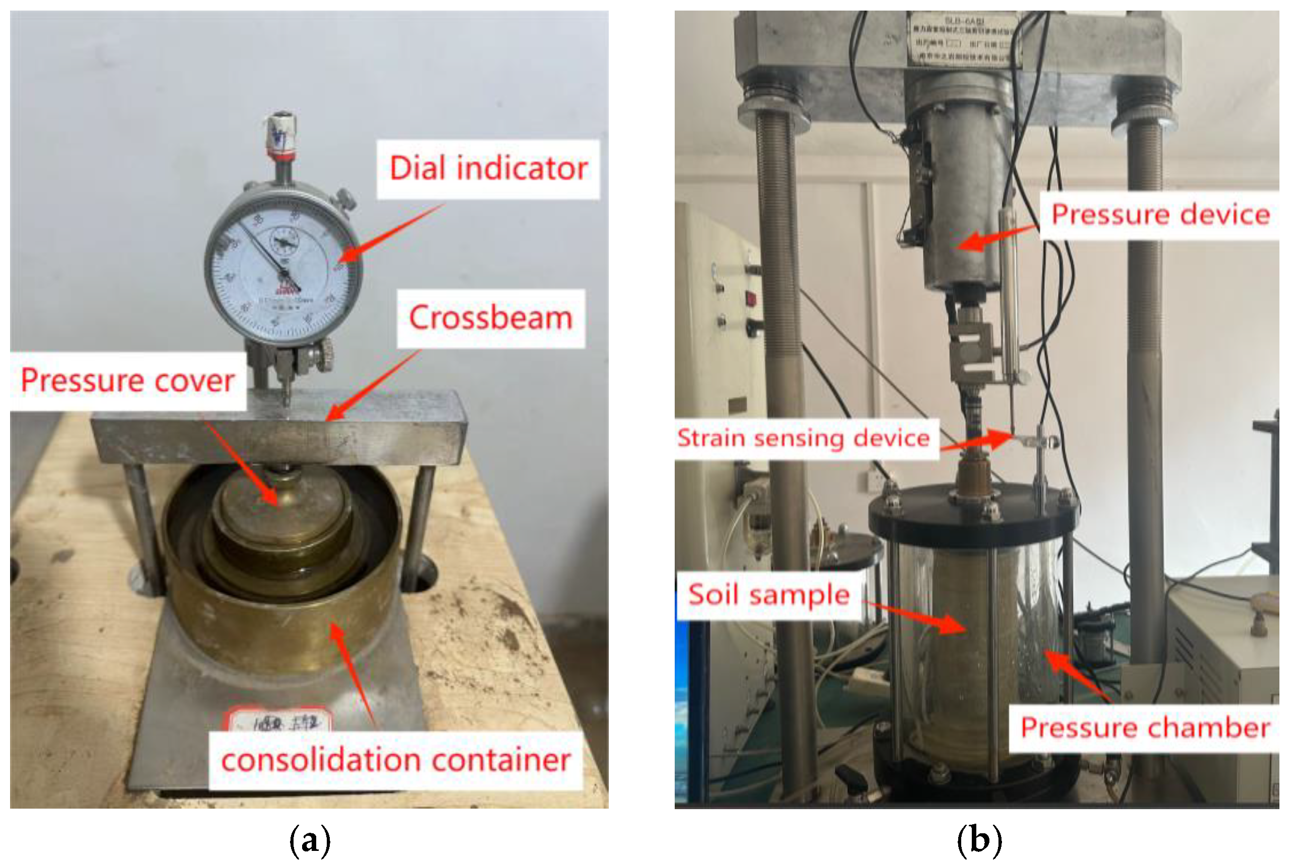
Standard consolidation test

(a)

In the consolidation container, the following were placed in order from bottom to top: large permeable stones, filter paper, a ring-knife containing the saturated soil sample (with the ring-knife facing downward), filter paper, and small permeable stones. Then, the guide ring was placed and covered with the pressure cap. The permeable stones and filter paper had been pre-soaked to moisten them.

(b)

Water was injected into the grooves around the ring-knife to ensure that the saturated sample remained unaffected by water evaporation during consolidation. During the test, the water in the grooves was replenished as needed.

(c)

The crossbeam used to apply vertical pressure was lowered, ensuring that the bolts at the bottom of the crossbeam were securely fitted into the concave holes on the upper part of the pressure cover. Then, the dial indicator was installed and adjusted to zero.

(d)

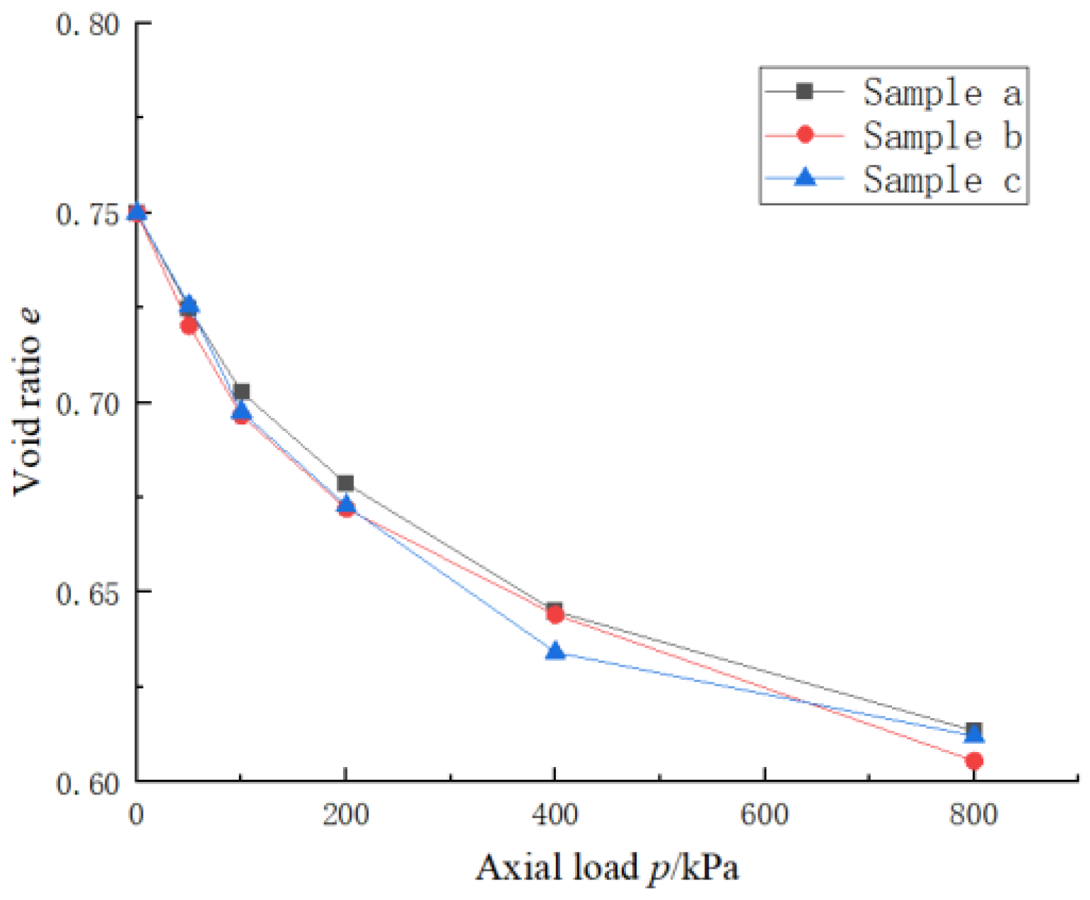
The vertical load was applied in five sequential stages: 50 kPa, 100 kPa, 200 kPa, 400 kPa, and 800 kPa. For each load level, the dial indicator reading was allowed to stabilize before the next load level was applied.

(e)

The readings of the dial indicator were recorded after each level of load had stabilized.

(2)

Triaxial consolidation drained shear test

(a)

Water-head saturation: The water head outside the pressure chamber was set to approximately 1 m higher than the top of the sample. Under the influence of gravitational potential energy, water gradually seeped upward from the bottom of the sample, while gas was expelled through the exhaust pipe at the top of the sample.

(b)

Back-pressure saturation: Water-head saturation often fails to fully saturate the sample, making back-pressure saturation necessary. The back pressure was set to 100 kPa, the confining pressure to 110 kPa, and the test duration to 3 h.

(c)

B-value detection: The back pressure and undrained conditions were kept unchanged, and the confining pressure was increased by 30 kPa. Then, the pore water pressure coefficient B was measured. When $B=\Delta u/\Delta \sigma >95\%$, the sample was considered saturated.

(d)

Consolidation: The back pressure was maintained at the level of the saturated back pressure, and the effective confining pressure was set to 100 kPa, meaning that the confining pressure was 100 kPa greater than the back pressure. The consolidation time was 1 to 2 days.

(e)

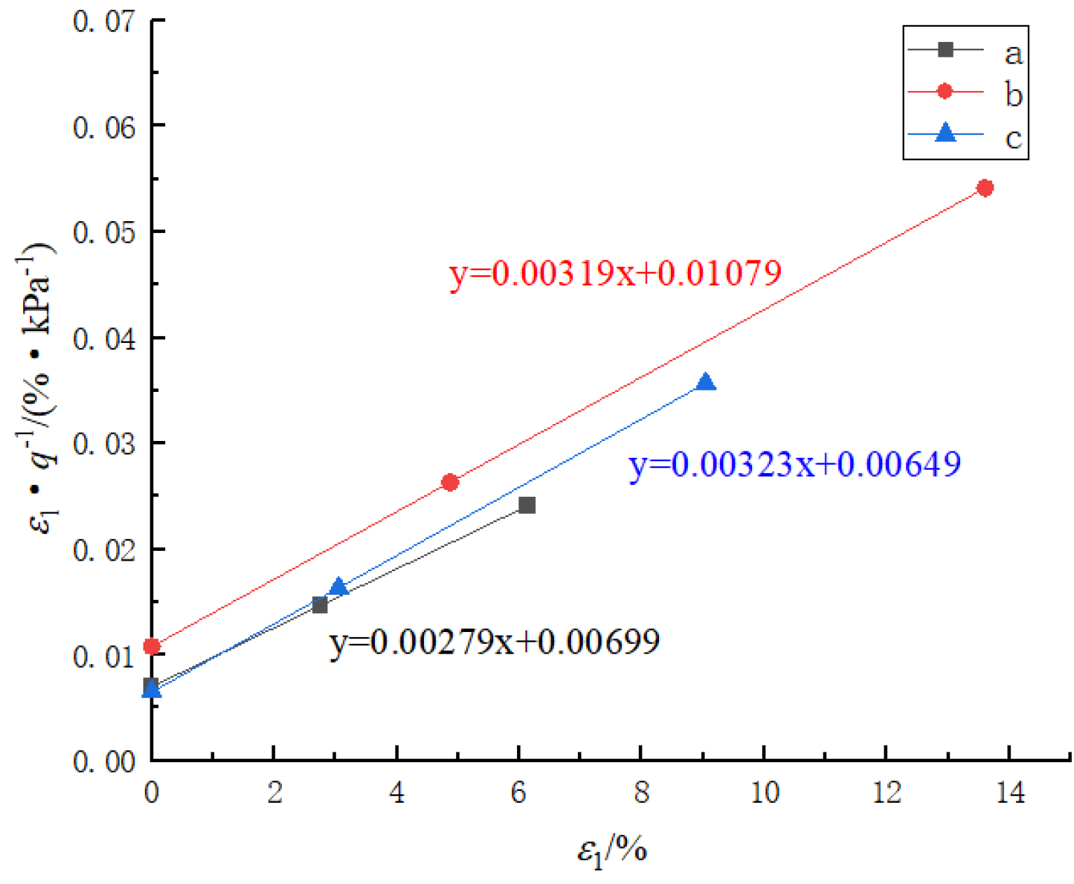
Drained shear: The confining pressure was kept constant, and the strain rate was controlled with an equal strain rate of 0.008 mm/min to ensure that the pore water in the sample was fully drained. The test was stopped when the strain of the sample reached 20% or when the sample exhibited significant strain softening.

(3)

Triaxial consolidation drained loading−unloading shear test

The only difference between the triaxial consolidation drained loading−unloading shear test and the triaxial consolidation drained shear test was in step (e).

Step (e): Loading−unloading shear: During the drained shear process, when the axial strain reached approximately 40% of the axial strain corresponding to the peak strength of the sample in the triaxial consolidated drained test, shearing was stopped and axial unloading was carried out to zero. After the unloading was complete, the drained shear process was repeated until the end of the test.

3.3. Tests Result

The reference tangent modulus $E_{\mathrm{oed}}^{\mathrm{ref}}$ and compression modulus $E_{\mathrm{s}1-2}$ of the soil sample were obtained through standard consolidation tests. Three parallel tests were conducted, and the relationship between the axial load and axial strain of the soil sample is presented in Figure 3. The fitted curve function R² for all three tests exceeded 0.99, resulting in $E_{\mathrm{oed}}^{\mathrm{ref}}$ values of 6.78, 6.86, and 6.41 MPa for the three soil samples, respectively, with an average value of 6.68 MPa.

Figure 4 illustrates the relationship between the void ratio and axial load in the standard consolidation test. Through parallel testing of samples a, b, and c, the compression moduli $E_{\mathrm{s}1-2}$ of the soil samples were determined to be 7.08 MPa, 6.93 MPa, and 6.84 MPa, respectively, with an average value of 6.95 MPa.

In Figure 5, the stress−strain relationship curves for soil samples a, b, and c obtained from the triaxial consolidation-drained shear tests are presented. From these curves, the failure values $q_{\mathrm{f}}$ and the reference secant modulus $E_{50}^{\mathrm{ref}}$ at the reference stress can be determined. The $q_{\mathrm{f}}$ values were set to the peak stress values, which were 268.0 kPa, 264.3 kPa, and 266.6 kPa, respectively. The value of $E_{50}^{\mathrm{ref}}$ is equal to the slope of the line connecting the origin of the coordinate system with the point on the curve corresponding to 0.5$q_{\mathrm{f}}$. These values were 8.75 MPa, 8.19 MPa, and 9.22 MPa, respectively, yielding an average $E_{50}^{\mathrm{ref}}$ value of 8.72 MPa.

In the definition of the HSS model, the axial strain ${\epsilon }_1$ has a hyperbolic relationship with the deviatoric stress q, as shown in Formula (1):

$${\epsilon }_1={\displaystyle \frac{1}{2E_{50}}}\cdot {\displaystyle \frac{q}{1-q/q_{\mathrm{a}}}}(q<q_{\mathrm{f}})$$

(1)

After transformation, a linear relationship between ${\epsilon }_1/q$ and ${\epsilon }_1$ can be obtained, as shown in Formula (2):

$${\displaystyle \frac{{\epsilon }_1}{q}}={\displaystyle \frac{{\epsilon }_1}{q_{\mathrm{a}}}}+{\displaystyle \frac{1}{2E_{50}}}(q<q_{\mathrm{f}})$$

(2)

Due to the difficulty of perfectly aligning the actual stress−strain relationship with a hyperbolic curve, the transformed ${\epsilon }_1/q$ − ${\epsilon }_1$ relationship curve will also deviate from linearity. To reduce human factors and perform a better linear fitting, the fitting line was made to pass through the points where the stress levels $q/q_{\mathrm{f}}$ were 70% and 95%, and the ${\epsilon }_1/q$ − ${\epsilon }_1$ relationship line was plotted [11] (as shown in Figure 6); by taking the reciprocal of the slope of this line, the asymptotic value $q_{\mathrm{a}}$ could be obtained, and the failure ratio $R_{\mathrm{f}}=q_{\mathrm{f}}/q_{\mathrm{a}}$, resulting in $R_{\mathrm{f}}$ values of 0.75, 0.84, and 0.86, with $R_{\mathrm{f}}$ set to 0.85.

To obtain the reference loading and unloading modulus $E_{\mathrm{ur}}^{\mathrm{ref}}$, triaxial consolidation drained loading and unloading tests were required. The stress−strain curve obtained during the loading and unloading test at the reference confining pressure $p^{\mathrm{ref}}=100$ kPa is shown in Figure 7. During the loading and unloading process, the test curve of the soil sample exhibited a hysteresis loop. Connecting the two endpoints of the hysteresis curve, the slope of the resulting straight line is the reference loading and unloading modulus of the soil sample. The $E_{\mathrm{ur}}^{\mathrm{ref}}$ values obtained from three sets of tests were 44.1 MPa, 41.7 MPa, and 43.4 MPa, with an average value of 43.1 MPa.

4. Selection of HSS Model Parameters

Through the above three parts of the test, the compression modulus $E_{\mathrm{s}1-2}$ of the soil sample can be obtained, as well as the small-strain moduli $E_{\mathrm{oed}}^{\mathrm{ref}}$, $E_{50}^{\mathrm{ref}}$, $E_{\mathrm{ur}}^{\mathrm{ref}}$ at the reference stress $p^{\mathrm{ref}}=100$ kPa, and the failure ratio $R_{\mathrm{f}}$. This allows us to determine the ratio of the soil sample’s compression modulus to its small-strain moduli, which is $E_{\mathrm{s}1-2}:E_{\mathrm{oed}}^{\mathrm{ref}}:E_{50}^{\mathrm{ref}}:E_{\mathrm{ur}}^{\mathrm{ref}}=1:0.96:1.25:6.2$.

The value of $G_0^{\mathrm{ref}}$ needs to be determined through resonant column tests; it can also be calculated using empirical formulas. The initial dynamic shear modulus of soil $G_0$ is also known as the maximum shear modulus $G_{\max }$; Hardin [21] provided an expression for $G_{\max }$ based on the soil’s initial void ratio $e_0$ through extensive tests, and this is Equation (3); after summarizing the effects of $e_0$ and confining pressure on $G_{\max }$, Hardin [22] improved this formula, thus obtaining Formula (4).

$$G_{\max }=33\times {\displaystyle \frac{{(2.97-e_0)}^2}{1+e_0}}$$

(3)

$$G_{\max }={\displaystyle \frac{A{(2.973-e)}^2}{1+e}}{({\displaystyle \frac{p^{\prime }}{p_a}})}^n$$

(4)

In the formula, $p^{\prime }$ represents the average effective confining pressure and $p_a$ is the reference confining pressure, typically equal to standard atmospheric pressure (100 kPa).

After considering the effect of moisture content on the initial dynamic shear modulus of loess, Jian Tao et al. [23] improved Hardin’s empirical Formula (4), and fitted the functions of A and n with respect to water content, making it more suitable for loess regions, as shown in Formulas (5) and (6).

$$A=129.094\times {(100w)}^{-0.364}$$

(5)

$$n=0.301{(100w)}^{0.060}$$

(6)

Gu Xiaoqiang [17] derived the fitting functions (7) and (8) between the void ratio e and $G_0^{\mathrm{ref}}$ based on field wave-speed tests.

$$G_0^{ref}=67.5e^{-1.57}$$

(7)

$$G_0^{ref}=98.9e^{-0.45}$$

(8)

In this context, Formula (7) is more suitable for clay, while Formula (8) is more suitable for sand.

In actual engineering practice, the initial dynamic shear modulus $G_0^{\mathrm{ref}}$ can also be determined based on empirical values. As can be seen from

Table 4. The modulus ratios of HSS models in different regions.

Region	Soil Sample	${\mathit{E}}_{\mathbf{oed}}^{\mathbf{ref}}/{\mathit{E}}_{\mathbf{s}}$	${\mathit{E}}_{50}^{\mathbf{ref}}/{\mathit{E}}_{\mathbf{oed}}^{\mathbf{ref}}$	${\mathit{E}}_{\mathbf{ur}}^{\mathbf{ref}}/{\mathit{E}}_{50}^{\mathbf{ref}}$	${\mathit{G}}_0^{\mathbf{ref}}/{\mathit{E}}_{\mathbf{ur}}^{\mathbf{ref}}$
Gaoxiong [17]	Sand	-	1	3	2.42
Tongchuan [24]	Loess	0.93	12.46	7.6	2.23
Xi’an [25]	Loess	1.77	1.61	5.29	1.73
Yan’an [26]	Loess	-	1.2	3	3
Jinan [27]	Clay	1	1	8	1.5
Jinan [28]	Silty clay	-	0.91	6.97	1.74
Shanghai [18]	Soft clay	0.63~1.06	1.08~1.2	6.7~11.6	0.8~1.2
Shanghai [29]	Clay	0.9	1.2	6~8	2.5~4.9
Wuhan [30]	Silty clay	0.7~0.8	0.7~1.5	3.7~5.8	2.1~3.0
Hangzhou [31]	Clay	0.92	1.18	6.53	2
Hangzhou [32]	Silty clay	0.73~1	1~2.22	5~8.97	1.3~3
Suzhou [33]	Silty clay, Silt	-	0.8	4	3.8~4.55
Yancheng [34]	Silty clay	0.84	1.5	5.56	1.57~1.73
Changzhou [35]	Clay, Silty clay	-	1.33~1.50	3.6~4.3	1.6~2.0
Paris, France [36]	Sand	-	1	2.5	1.89
London, Britain [37]	Clay	-	2	5.3	4.16
Lisbon, Portugal [38]	Stiff clay	-	1	3	2.3
Jurmala, Latvia [39]	Subglacial till	-	1	3	2.96
Incheon, South Korea [40]	Sediment	-	1.25	3	2.65
Ledsgård, Sweden [41]	Clay	-	1	3	2.53~3.03

, the value of $G_0^{\mathrm{ref}}$ in various regions generally ranges from 1.5 to 5 times that of the $E_{\mathrm{ur}}^{\mathrm{ref}}$. In loess regions, the ratio $G_0^{\mathrm{ref}}/E_{\mathrm{ur}}^{\mathrm{ref}}$ typically falls between 1.5 and 3.

However, since the value of $G_0^{\mathrm{ref}}$ has a significant impact on the prediction generated by the numerical simulation, this paper will further analyze the value of $G_0^{\mathrm{ref}}$ in the loess region.

The coefficient of earth pressure at rest $K_0$ can be obtained through stress-path triaxial tests, and some geological survey reports may also provide it. However, in practical applications, it is usually calculated using empirical formulas, such as those for clay ($K_0=0.95-\sin {\phi }^{\prime }$) and for sand ($K_0=1-\sin {\phi }^{\prime }$). According to the theory of elasticity, it can also be calculated using Poisson’s ratio $\nu$ (see Formula (9)):

$$K_0=\nu /(1-\nu )$$

(9)

Gu Xiaoqiang et al. [19] established the relationship between $K_0$ and the void ratio e based on indoor tests. For cohesive soils, the relationship is as expressed in Formula (10), while for sandy soils, it is as shown in Formula (11):

$$K_0=0.049e+0.02I_{\mathrm{p}}+0.139$$

(10)

$$K_0=0.154e+0.224$$

(11)

In the formulas mentioned, $I_{\mathrm{p}}$ represents the plasticity index.

Since Formulas (10) and (11) are derived from the $K_0$ test values of typical soils in the Shanghai area, they are subject to regional limitations. Shanghai is characterized by soft clay soil, the mechanical properties of which may differ significantly from those of loess in the Xi’an area.

Wang Yu-chuan [42] obtained the fitting formula for $K_0$ of loess by fitting it with the over-consolidation ratio (OCR), as in Formula (12):

$$K_{OCR}=0.42\times OC{R}^{0.36}$$

(12)

Due to the significant influence of water content and stress history on the $K_0$ value of loess, Formulas (10) and (11), provided by Gu Xiaoqiang, do not account for the impact of stress history. Although Formula (12) is a fitting formula specifically for loess, it also fails to consider the effects of water content w and void ratio e. Consequently, using these formulas to calculate the $K_0$ value of loess may lead to some deviation.

This article fits the water content w, void ratio e, over-consolidation ratio, and the coefficient of earth pressure at rest $K_0$ for loess, resulting in Formula (13):

$$K_0=1.4w+0.033e+0.11OC{R}^{-0.28}$$

(13)

The deviation between the $K_0$ calculated using this formula and the experimental results does not exceed 15%, as shown in Figure 8. This indicates that Equation (13) is more suitable than the previous equation for calculating the $K_0$ of loess.

Other parameters can be determined based on the geological survey report and relevant research experience.

m was set to 0.75.

The value of $\psi$ can be set according to Bolton’s [43] recommendation: for sandy soil, $\psi ={\phi }^{\prime }-30°$, and when ${\phi }^{\prime }<30°$, $\psi$ is set to 0; for clayey soil, $\psi$ is set to 0.

Based on soil parameters in Shanghai, when the void ratio e is less than 1.0, $R_{\mathrm{f}}$ is set to 0.95. However, Zhong Peng [24] suggests that for loess, $R_{\mathrm{f}}$ should be between 0.8 and 0.9. This article, based on the results of tests, set $R_{\mathrm{f}}$ to 0.85.

When there are no experimental data available, $v_{\mathrm{ur}}$ can be set according to the recommended value in the PLAXIS (version, 20.1.0.98) manual, which is 0.2.

${\gamma }_{0.7}$ can be set in the range $1\times {10}^{-4}$ to $4\times {10}^{-4}$ [44,45]. This article used the value $2\times {10}^{-4}$.

5. Engineering Verification

5.1. Project Overview

The proposed construction of the Xi’an Metro Line 15, from Shenzhou 2nd Road Station to East Chang’an Street Station, involves tunneling beneath the Heihe River water-supply pipeline (Phase II, single pipe). The right line is 1018.923 m long, and the left line is 1018.952 m long (including a short chain of 0.271 m). Both the left and right lines feature a single slope, with maximum gradients of 30.147‰ and 30.138‰, respectively. The burial depth of the tunnel arch top ranges from 19.94 m to 43.55 m, and the stable water-level burial depth is between 21 m and 35.8 m. The surrounding rock and soil are mainly classified as Class IV and Class V surrounding rocks. The minimum net distance between the shield-tunnel structure and the Heihe pipeline is only 3.867 m. The Heihe River water-supply pipeline has been in service for more than 20 years; it has low structural strength and is easily damaged due to long-term neglect. During the tunneling process, it is necessary to strictly control the disturbance to the water pipeline.

Figure 9 is a plan view of the relationship between the tunnel and the water pipeline. Figure 10 shows the internal view after tunnel construction.

The geological survey report provided soil-layer parameters, as shown in

Table 5. Partial physical and mechanical parameters of soil.

Soil Layer Name	Unit Weight	Natural Water Content	Void Ratio	Over-Consolidation Ratio	Compression Modulus	Consolidated Quick Shear Test
						Cohesion	Internal Friction Angle
	$\mathit{\gamma }$	w	e	OCR	${\mathit{E}}_{\mathbf{s}}$	c	$\mathit{\phi }$
	$\mathbf{kN}\cdot {\mathbf{m}}^{-3}$	%	-	-	MPa	kPa	$°$
I Plain Fill	15.7	-	-	-	-	0	5.0
II 3-1 New Loess	16.97	19.5	0.887	2.41	10.1	34.0	23.5
III 3-2 Paleosol	18.52	18.7	0.713	1.34	11.2	34.0	24.0
IV 4-1-1 Old Loess	16.87	21.2	0.925	1.30	9.7	34.0	24.0
V 4-1-2 Old Loess	19.52	21.2	0.768	1.03	6.6	33.5	22.5
VI 4-2-2 Old Loess	19.72	24.1	0.688	1.01	7.5	34.0	24.0

.

5.2. Modeling

Using the PLAXIS 3D finite element software for modeling, this study analyzed the left line tunnel passing beneath the Heihe River water-supply pipeline. The geometric dimensions of the model are 70 m × 90.5 m × 70 m. The tunnel has a circular cross-section with an inner diameter of 5.5 m and an outer diameter of 6.2 m. The cross-section of the Heihe River phase 2 water-supply pipeline is horseshoe-shaped, with a width of 2.5 m, a height of 2.5 m, and a wall thickness of 0.3 m. The model structure is shown in Figure 11. Considering the properties of various materials, the plain fill is modeled using the Mohr-Coulomb model, while the concrete lining of the tunnel and the water-supply pipeline are modeled using the linear elastic model. All other soil types are modeled with the HSS model.

The partial parameters of the HSS model for each soil layer are shown in

Table 6. Partial parameters of HSS model.

Soil Layer Name	${\mathit{E}}_{\mathbf{oed}}^{\mathbf{ref}}/\mathbf{MPa}$	${\mathit{E}}_{50}^{\mathbf{ref}}/\mathbf{MPa}$	${\mathit{E}}_{\mathbf{ur}}^{\mathbf{ref}}/\mathbf{MPa}$	${\mathit{K}}_0$
II 3-1 New Loess	9.7	12.6	62.6	0.40
III 3-2 Paleosol	10.8	14	69.4	0.39
IV 4-1-1 Old Loess	9.3	12.1	60.1	0.43
V 4-1-2 Old Loess	6.3	8.3	40.9	0.43
VI 4-2-2 Old Loess	7.2	9.4	46.5	0.47

.

The basic parameters of the concrete lining for tunnels and the Heihe Water Pipeline are shown in

Table 7. The table of concrete lining.

Structure	Thickness	Unit Weight	Elastic Modulus	Poisson’s Ratio
	m	$\mathbf{kN}\cdot {\mathbf{m}}^{-3}$	GPa	-
Lining of tunnel	0.35	24.1	34.5	0.2
Lining of Heihe Water Pipeline	0.3	23.5	25.5	0.2

.

5.3. Analysis of Simulated Result

Numerical simulations were conducted using the HSS model, HS model, and M−C model for the shield tunnel passing beneath the Heihe River phase 2 water-supply pipeline. For the simulation using the HSS model, calculations were performed based on the improved Formulas (4), (7) and (8), as well as on results with $1.5E_{\mathrm{ur}}^{\mathrm{ref}}$, $2E_{\mathrm{ur}}^{\mathrm{ref}}$, and $3E_{\mathrm{ur}}^{\mathrm{ref}}$ multipliers. The simulation results were compared and verified against on-site monitoring data, as shown in Figure 12a. The comparison between the calculation results of the M−C and HS models and the field monitoring data is presented in Figure 12b.

As the shield tunnel advances, the settlement at the center of the bottom of the Heihe River water-supply pipeline gradually increases. The maximum value monitored on-site is 2.5 mm. The maximum settlement value simulated by the M−C model is 13.6 mm, while the maximum settlement simulated by the HSS model when $G_0^{\mathrm{ref}}=1.5E_{\mathrm{ur}}^{\mathrm{ref}}$ is 4.1 mm. It can be seen that the HSS model fits the on-site monitoring data better than the M−C and HS models. The engineering requirement is that the cumulative settlement of the Heihe River water pipeline must not exceed 8 mm. It is evident that the calculation results of the M−C and HS models are overly conservative, and the accuracy of these results no longer meets the needs of this project.

Among the various methods of determining the value of $G_0^{\mathrm{ref}}$, the simulation results from the three empirical formulas are similar, but all are lower than the on-site monitoring data. When $G_0^{\mathrm{ref}}$ is set to $2E_{\mathrm{ur}}^{\mathrm{ref}}$, the simulation results from the HSS model are the closest to the on-site monitoring data, and the settlement values obtained from the simulation are slightly greater than the monitoring data, which could be more conducive to construction safety.

6. Conclusions

This article obtained several parameters of the HSS model for Xi’an loess through indoor tests, established proportional relationships between the parameters, and vali-dated them using engineering examples. The conclusions are as follows:

(1)

The proportional relationship between the small-strain moduli in the HSS model for Xi’an loess was obtained through indoor tests. Numerical simulations were performed for various values of the initial dynamic shear modulus $G_0^{\mathrm{ref}}$. Through a comparison of the simulation results with the field monitoring data, it was found that when the ratio of $E_{\mathrm{s}1-2}$, $E_{\mathrm{oed}}^{\mathrm{ref}}$, $E_{50}^{\mathrm{ref}}$, $E_{\mathrm{ur}}^{\mathrm{ref}}$ and $G_0^{\mathrm{ref}}$ in the HSS model is 1:0.96:1.25:6.2:12.4, and $R_{\mathrm{f}}=0.85$, the simulation results are closest to the field monitoring data. This can provide a reference for similar engineering analyses in the Xi’an loess region.

(2)

By fitting the data, a functional relationship between the coefficient of earth pressure at rest $K_0$ and the water content w, void ratio e, and over-consolidation ratio OCR for loess was established. The deviation between the values calculated using this fitting formula and the test data is within 15%, providing an empirical method for determining the K value of Xi’an loess.

(3)

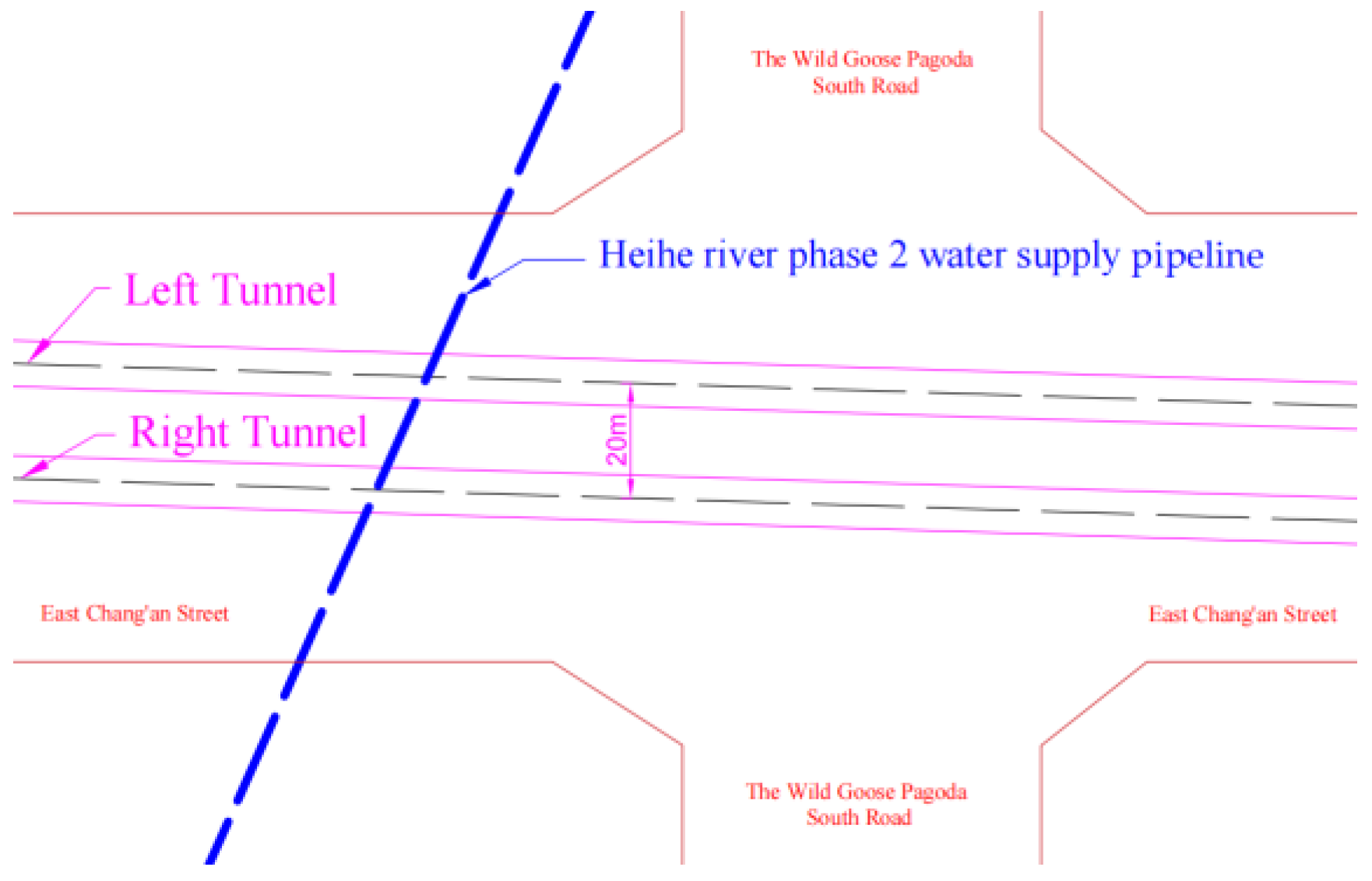
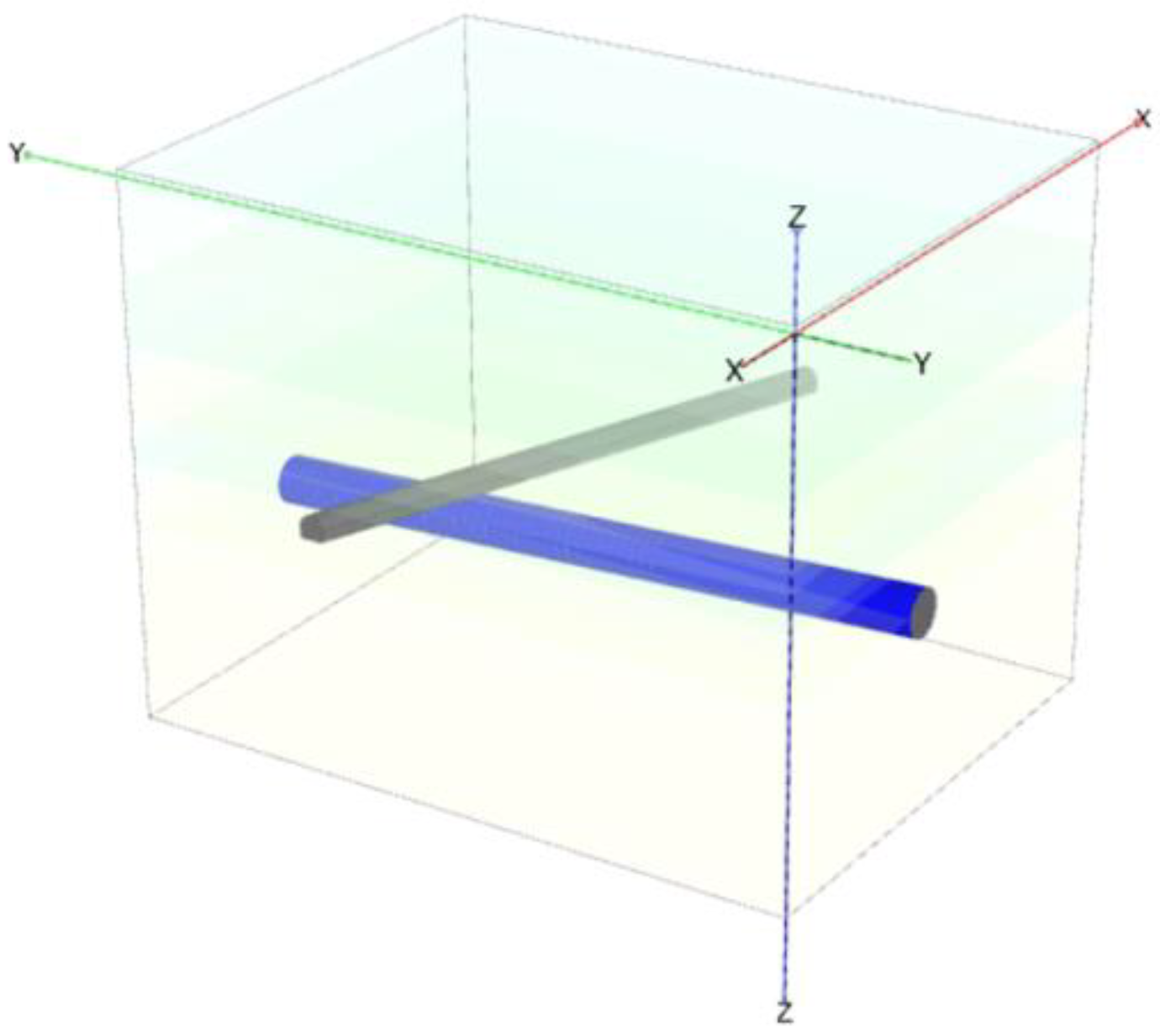
Through numerical analysis of the section between Shen Zhou 2nd Road Station and Dong Chang’an Street Station on Xi’an Metro Line 15, it was found that compared to the M−C and HS models, the HSS model results are closer to the field monitoring data. The HSS model is more suitable for projects with stricter settlement requirements, and it also validates the feasibility of applying the HSS parameters proposed in this paper.

(4)

The above conclusions are derived from the study of loess in the Xi’an area, and further research is needed to determine whether they are applicable to loess in other regions. Future studies will conduct experiments on loess from more regions and at different depths to analyze and summarize the patterns of HSS model parameters for loess in various areas.

References

1. Jafari, M. System identification of a soil tunnel based on a hybrid artificial neural network–numerical model approach. Iran. J. Sci. Technol.-Trans. Civ. Eng. 2020, 44, 560–572. [Google Scholar] [CrossRef]
2. Zhao, X.; Li, Z.; Dai, G.; Wang, H.; Yin, Z.; Cao, S. Numerical Study on the Effect of Large Deep Foundation Excavation on Underlying Complex Intersecting Tunnels. Appl. Sci. 2022, 12, 4530. [Google Scholar] [CrossRef]
3. Han, Y.; Ye, W.; Wei, Q. Research on the Influence of New Shield Tunnel to Adjacent Existing Tunnel. Appl. Mech. Mater. 2013, 295–298, 2985–2989. [Google Scholar] [CrossRef]
4. Zhang, Z.; Huang, M. Geotechnical influence on existing subway tunnels induced by multiline tunneling in Shanghai soft soil. Comput. Geotech. 2014, 56, 121–132. [Google Scholar] [CrossRef]
5. Atkinson, J.; Sallförs, G. Experimental determination of stress-strain-time characteristics in laboratory and in-situ tests. General Report. In Proceedings of the 10th European Conference on Soil Mechanics and Foundation Engineering, Florence, Italy, 26–30 May 1991; pp. 915–956. [Google Scholar]
6. Wang, Z.; Wang, H.; Qi, K.; Zai, J. Summary and evaluation of experimental investigation on small strain of soil. Rock Soil Mech. 2007, 28, 1518–1524. [Google Scholar]
7. Burland, J. Ninth Laurits Bjerrum Memorial Lecture: “Small is beautiful”—The stiffness of soils at small strains. Can. Geotech. J. 1989, 26, 499–516. [Google Scholar] [CrossRef]
8. Attewell, P.; Farmer, I. Ground deformations resulting from shield tunnelling in London Clay. Can. Geotech. J. 1974, 11, 380–395. [Google Scholar] [CrossRef]
9. Mair, R. Developments in geotechnical engineering research: Application to tunnels and deep excavations. In Proceedings of the Institution of Civil Engineers, London, UK, 20 January 1993; pp. 27–41. [Google Scholar]
10. Zheng, G.; Yang, X.; Zhou, H.; Du, Y.; Sun, J.; Yu, X. A simplified prediction method for evaluating tunnel displacement induced by laterally adjacent excavations. Comput. Geotech. 2018, 95, 119–128. [Google Scholar] [CrossRef]
11. Ardakani, A.; Bayat, M.; Javanmard, M. Numerical modeling of soil nail walls considering Mohr Coulomb, hardening soil and hardening soil with small-strain stiffness effect models. Geomech. Eng. 2014, 6, 391–401. [Google Scholar] [CrossRef]
12. Mu, L.; Huang, M. Small strain based method for predicting three-dimensional soil displacements induced by braced excavation. Tunn. Undergr. Space Technol. Inc. Trenchless Technol. Res. 2016, 52, 12–22. [Google Scholar] [CrossRef]
13. Zhang, R.; Zhang, W.; Goh, A. Numerical investigation of pile responses caused by adjacent braced excavation in soft clays. Int. J. Geotech. Eng. 2018, 15, 783–797. [Google Scholar] [CrossRef]
14. Zhang, J.; Zhao, G.; Zhang, L.; Jiang, H. Application of HSS Model in Shield Simulation and Parameter Sensitivity Research. Chin. J. Undergr. Space Eng. 2020, 16, 618–625. [Google Scholar]
15. Xiao, S.; Xu, M.; Lan, R. Choice of Soil Constitutive Models in Numerical Analysis of Foundation Pit Excavation Based on FLAC3D. In Proceedings of the 2023 International Conference on Green Building, Civil Engineering and Smart City (GBCESC 2023); Lecture Notes in Civil Engineering. Springer: Singapore, 2023; Volume 328. [Google Scholar] [CrossRef]
16. Wang, T.; Deng, T.; Deng, Y.; Yu, X.; Zou, P.; Deng, Z. Numerical Simulation of Deep Excavation Considering Strain-Dependent Behavior of Soil: A Case Study of Tangluo Street Station of Nanjing Metro. Int. J. Civil. Eng. 2023, 21, 541–550. [Google Scholar] [CrossRef]
17. Hsiung, B.; Dao, S. Evaluation of Constitutive Soil Models for Predicting Movements Caused by a Deep Excavation in Sands. Electron. J. Geotech. Eng. 2014, 19, 17325–17345. [Google Scholar]
18. Liang, F.; Jia, Y.; Ding, Y.; Huang, M. Experimental study on parameters of HSS model for soft soils in Shanghai. Chin. J. Geotech. Eng. 2017, 39, 269–278. [Google Scholar]
19. Gu, X.; Wu, R.; Liang, F.; Gao, G. On HSS model parameters for Shanghai soils with engineering verification. Rock Soil Mech. 2021, 42, 833–845. [Google Scholar]
20. Benz, T. Small Strain Stiffness of Soils and Its Numerical Consequences. Ph.D. Thesis, University of Stuttgart, Stuttgart, Germany, 2006. [Google Scholar]
21. Hardin, B.O.; Black, W.L. Closure to “Vibration Modulus of Normally Consolidated Clay”. J. Soil. Mech. Found. Div. 1969, 95, 1531–1537. [Google Scholar] [CrossRef]
22. Hardin, B.O.; Drnevich, V.P. Shear Modulus and Damping in Soils: Design Equations and Curves. J. Soil. Mech. Found. Division. 1972, 98, 667–692. [Google Scholar] [CrossRef]
23. Jian, T.; Kong, L.; Bo, W.; Wang, J.; Liu, B. Experimental study on the influence of water content on the small strain shear modulus of undisturbed loess. Chin. J. Geotech. Eng. 2022, 44, 160–165. [Google Scholar]
24. Zhong, P. Research on Deformation Characteristics of Loess Foundation Pit Excavation Based on HSS Model. Master’s Thesis, Chang’an University, Xi’an, China, 2023. [Google Scholar]
25. Liu, D. Parameter Inversion of Small Strain Hardened Soil Constitutive Model Based on GA-BP and Its Application in Foundation Pit Engineering. Master’s Thesis, Chang’an University, Xi’an, China, 2022. [Google Scholar]
26. Liao, J.; Zhu, Q.; Wang, Z.; Dai, Z. Comparison of Simulating Loess Deformation by Two Advanced and Conventional Constitutive Models. Chin. J. Undergr. Space Eng. 2023, 19, 784–792. [Google Scholar]
27. Li, L.; Liu, J.; Li, K.; Huang, H.; Ji, X. Study of parameters selection and applicability of HSS model in typical stratum of Jinan. Rock Soil Mech. 2019, 40, 4021–4029. [Google Scholar] [CrossRef]
28. Lu, Y. Research on the Impact and Control Measures of Shield Tunnel Construction on Adjacent Bridges Based on HSS Model; University of Jinan: Jinan, China, 2018. [Google Scholar]
29. DG/TJ 508–61–2018; Technical Code for Excavation Engineering. Tongji University Press: Shanghai, China, 2018.
30. Xu, W.; Liu, C.; Hu, K.; Fan, Y.; Tai, J.; Ren, X.; Feng, X. Experimental study on parameters of hardening soil small-strain model for soft soil in Wuhan. Saf. Environ. Eng. 2024, 31, 88–99. [Google Scholar] [CrossRef]
31. Lin, D. Experimental Study and Engineering Application of Small Strain Soil Hardening Model Parameters. Master’s Thesis, Zhejiang University, Zhejiang, China, 2022. [Google Scholar] [CrossRef]
32. Meng, R. Parameter tests and engineering applications of small-strain hardening soil model of mucky silty clay in Hangzhou. J. Chengdu Univ. Technol. Sci. Technol. Ed. 2024, 51, 303–315. [Google Scholar]
33. Lu, T.; Liu, S.; Cai, G.; Wu, K.; Li, Z. Method and application of parameter determination for small strain hardened soil model based on SCPTU testing. J. Ground Improv. 2023, 5, 451–459. [Google Scholar]
34. Wang, X.; Gu, X.; Liu, H.; Lai, H.; Wu, C. Experimental Study on Main Parameters of HSS Model for Marine Soil in Dafeng Sea Area, Jiangsu Province. Mech. Eng. 2024, 46, 316–322. [Google Scholar]
35. Dong, X.; Zhou, F.; Zhu, R.; Wang, X.; Zeng, L. Sensitivity analysis and determination method of parameters for small strain soil hardening model. Sci. Technol. Eng. 2024, 24, 6366–6376. [Google Scholar]
36. Rafa, S. Cyclic lateral response of piles in dry sand: Effect of pile slenderness. In Proceedings of the Seventh International Jordanian Civil Engineering Conference (JICEC07) Reconstruction of Damaged Zones “The Role of Civil Engineering”, Chengdu, China, 9–11 May 2017. [Google Scholar]
37. Brinkgreve, R.B.J.; Kappert, M.H.; Bonnier, P.G. Hysteretic damping in a small-strain stiffness model. Environ. Sci. 2007, 737–742. Available online: https://www.researchgate.net/profile/R-Brinkgreve/publication/267411874_Hysteretic_damping_in_a_small-strain_stiffness_model/links/54b4edbc0cf26833efd0453b/Hysteretic-damping-in-a-small-strain-stiffness-model.pdf (accessed on 2 November 2024).
38. Fernando, S. Importance of small-strain stiffness on the prediction of the displacements of a flexible retaining wall on stiff clay. In Proceedings of the 17th European Conference on Soil Mechanics and Geotechnical Engineering, ECSMGE 2019—Proceedings, Reykjavik, Iceland, 1–6 September 2019. [Google Scholar]
39. Peteris, S.; Kaspars, B. Applicability of Small Strain Stiffness Parameters for Pile Settlement Calculation. Procedia Eng. 2017, 172, 999–1006. [Google Scholar] [CrossRef]
40. Kima, T.; Jung, Y. Optimizing Material Parameters to Best Capture Deformation Responses in Supported Bottom-up Excavation: Field Monitoring and Inverse Analysis. KSCE J. Civ. Eng. 2022, 26, 3384–3401. [Google Scholar] [CrossRef]
41. Jesús, F.; Cláudio, P. Non-linear critical speed in high-speed ballasted railways with ground reinforcement. Transp. Geotech. 2024, 48, 101325. [Google Scholar]
42. Wang, Y. Study on Triaxial Shear Characteristics of Loess Under K0 Consolidation Conditions. Master’s Thesis, Chang’an University, Xi’an, China, 2023. [Google Scholar] [CrossRef]
43. Bolton, M. The strength and dilatancy of sands. Géotechnique 1986, 36, 65–78. [Google Scholar] [CrossRef]
44. Zhang, W.; Goh, A.; Feng, X. A simple prediction model for wall deflection caused by braced excavation in clays. Comput. Geotech. 2015, 63, 67–72. [Google Scholar] [CrossRef]
45. Brinkgreve, R.; Kumarswamy, S.; Swolfs, W. PLAXIS Version 2015 Manual. The Netherlands. 2015. Available online: https://pdfcoffee.com/plaxis-10-pdf-free.html (accessed on 2 November 2024).
Figure 1. Strain limits for soil under conditions associated with various geotechnical engineering projects.
Applsci 15 01278 g001
Figure 2. Photos of instruments used in the tests.
Applsci 15 01278 g002
Figure 3. Relationships between axial load and axial strain, as determined by the standard consolidation test.
Applsci 15 01278 g003
Figure 4. Relationship between void ratio and axial load diagram, as determined by the standard consolidation test.
Applsci 15 01278 g004
Figure 5. Stress−strain relationship based on the triaxial test.
Applsci 15 01278 g005
Figure 6. Curve graph of the relationship between ε 1 / q and ε 1 .
Applsci 15 01278 g006
Figure 7. Stress−strain curves of the triaxial loading and unloading test.
Applsci 15 01278 g007
Figure 8. Comparison chart between K0 calculated by various formulas and test results.
Applsci 15 01278 g008
Figure 9. Plane diagram of the relationship between the tunnel and the Heihe River phase 2 water-supply pipeline.
Applsci 15 01278 g009
Figure 10. Internal photo of tunnel.
Applsci 15 01278 g010
Figure 11. Model structure diagram.
Applsci 15 01278 g011
Figure 12. Variations in the bottom centerline settlement of the Heihe water pipeline due to shield tunneling. (a) The settlement prediction results of the HSS model under different values of G0. (b) The prediction results of the HS model and M-C model.
Applsci 15 01278 g012