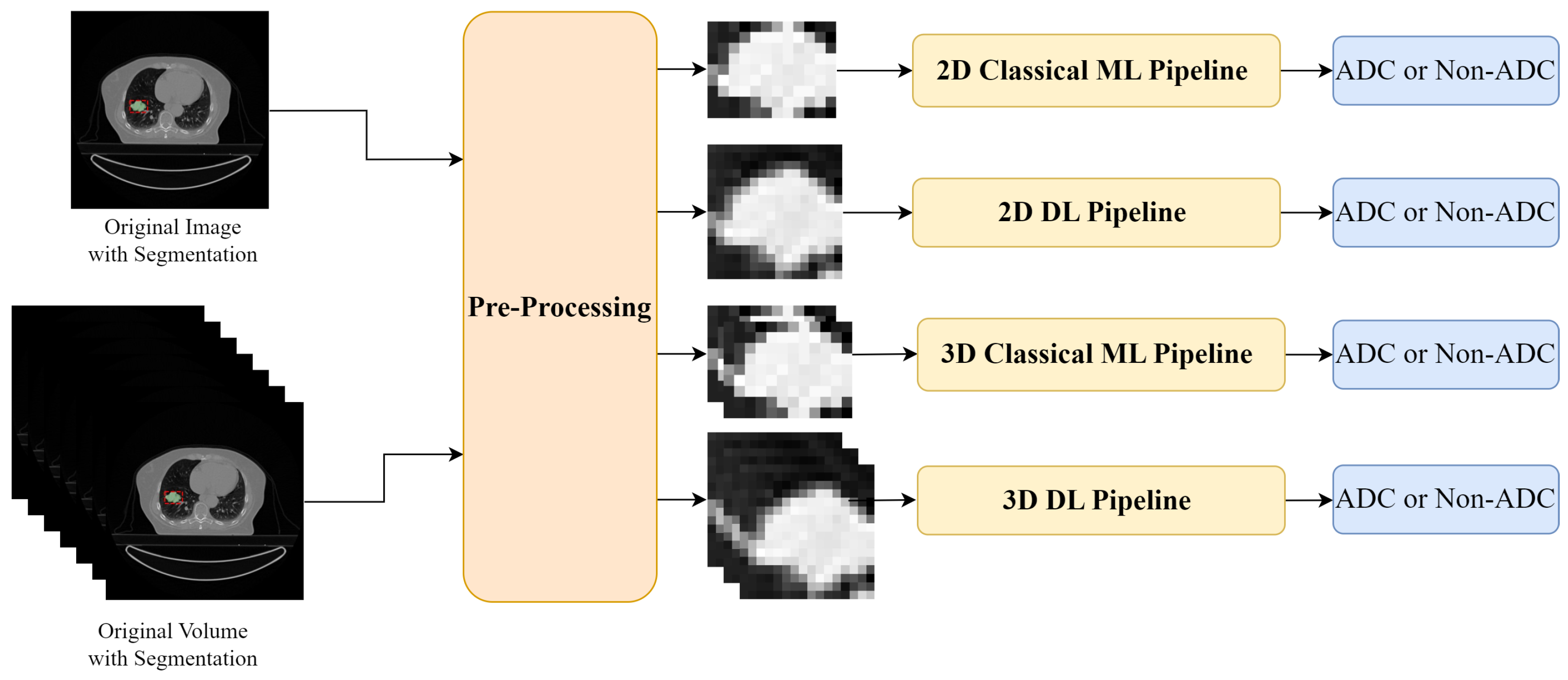
Article

Comparing 2D and 3D Feature Extraction Methods for Lung Adenocarcinoma Prediction Using CT Scans: A Cross-Cohort Study

by
Margarida Gouveia
1,2,*,†,
Tânia Mendes
1,2,*,†,
Eduardo M. Rodrigues
1,3,
Hélder P. Oliveira
1,3 and
Tania Pereira
1,4
1
Institute for Systems and Computer Engineering, Technology and Science (INESC TEC), 4200-465 Porto, Portugal
2
Faculty of Engineering, University of Porto (FEUP), 4200-465 Porto, Portugal
3
Faculty of Science, University of Porto (FCUP), 4169-007 Porto, Portugal
4
Faculty of Sciences and Technology, University of Coimbra (FCTUC), 3004-516 Coimbra, Portugal
*
Authors to whom correspondence should be addressed.
These authors contributed equally to this work.
Appl. Sci. 2025, 15(3), 1148; https://doi.org/10.3390/app15031148
Submission received: 8 November 2024 / Revised: 15 January 2025 / Accepted: 16 January 2025 / Published: 23 January 2025

Simple Summary

The identification of tumour histology, often requires invasive procedures and is essential for determining the optimal treatment plan for lung cancer patients. This study explores non-invasive methodologies for classifying lung adenocarcinoma, the most common subtype of lung cancer. Two primary approaches were studied: one based on radiomic features and the other utilizing deep features, extracted from computed tomography scans. Additionally, the study compares the use of 2D and 3D input data, as well as the performance of different classifiers, including Random Forest, eXtreme Gradient Boosting, Residual Neural Networks, and Hybrid Vision Transformers. The models were trained on a publicly available dataset and evaluated on two external public datasets. The results highlight the potential of these models for accurate classification while emphasizing the critical importance of evaluating models on external datasets.

Abstract

Lung cancer stands as the most prevalent and deadliest type of cancer, with adenocarcinoma being the most common subtype. Computed Tomography (CT) is widely used for detecting tumours and their phenotype characteristics, for an early and accurate diagnosis that impacts patient outcomes. Machine learning algorithms have already shown the potential to recognize patterns in CT scans to classify the cancer subtype. In this work, two distinct pipelines were employed to perform binary classification between adenocarcinoma and non-adenocarcinoma. Firstly, radiomic features were classified by Random Forest and eXtreme Gradient Boosting classifiers. Next, a deep learning approach, based on a Residual Neural Network and a Transformer-based architecture, was utilised. Both 2D and 3D CT data were initially explored, with the Lung-PET-CT-Dx dataset being employed for training and the NSCLC-Radiomics and NSCLC-Radiogenomics datasets used for external evaluation. Overall, the 3D models outperformed the 2D ones, with the best result being achieved by the Hybrid Vision Transformer, with an AUC of 0.869 and a balanced accuracy of 0.816 on the internal test set. However, a lack of generalization capability was observed across all models, with the performances decreasing on the external test sets, a limitation that should be studied and addressed in future work.

1. Introduction

According to the World Health Organization (WHO), lung cancer is both the most common and the most lethal form of cancer globally. In 2022, worldwide, 2.5 million new cases were registered and 1.80 million deaths were attributed to lung cancer [1]. Population growth and ageing lead to the rapid growth of diagnosed cancers and cancer-caused mortality [2]. The most common risk factors, namely air pollution, genetic predispositions, history of respiratory diseases and smoking, also contribute to this growth [3]. These several factors can interact, resulting in a pathological ecosystem with a complex causal process that affects prevention and patient therapeutic, in similarity with other types of cancer [4]. Lung cancer tumours can be divided into two histological groups: non-small-cell lung cancer (NSCLC) and small-cell lung cancer (SCLC). NSCLC is the most prevalent type of lung cancer, with an occurrence of 80% to 85% [3]. This type of cancer is divided into three different subtypes: adenocarcinoma (ADC), with a prevalence of 40%; squamous cell carcinoma (SCC), with a prevalence of 25%; and large cell carcinoma (LCC), responsible for 15% of the cases [3]. The less common subtypes, which have different characteristics from the aforementioned subtypes, can be aggregated in the “not otherwise specified” (NOS) subtype which accounts for 20% of the cases [5]. The prognosis and treatment of a malignant nodule can be impacted by the age and general health of the patient, cancer stage, tumour genetics, size, and subtype [5,6]. The histological subtype directly conditions the patient management, treatment, and survival [6,7,8]. For this reason, determining the tumour subtype can be of crucial importance and is performed by biopsies or by the pathological analysis of tissue recovered during resection surgery. This is an invasive procedure for the patient and a costly time-consuming process for the pathologist and sometimes requires the processing of multiple samples due to tumour heterogeneity [5,6]. The importance of the subtype identification process for patient treatment and prognosis demands a non-invasive method capable of being an alternative to a tissue biopsy. The use of CT scans does not impact the clinical workflow since these types of scans must be performed before the biopsies for localizing the lung nodules.
Currently, in clinical routine practice, the non-invasive imaging method used for the diagnosis and location of tumours, even small ones, is computed tomography (CT). Different tumour subtypes can be found in the CT image with different phenotype characteristics, such as size, morphology, margin irregularity or tumour opacity, which can be used to classify the tumour subtype and malignancy [5,9,10]. This classification task is, however, very reader-dependent and influenced by the knowledge, experience, and analytical skills of the radiologists [5,9]. This reveals the need for an automatic process capable of supporting radiologists to perform tumour classification with high accuracy and through a non-invasive procedure. The use of lung CT images allows the construction of predictive models capable of classifying the tumour subtype, which can be incorporated into the clinical workflow to support the decisions of radiologists [11].
This work aims to study how lung CT images can be used to construct a machine learning (ML) model capable of predicting lung tumour histological subtypes. The high predominance of the adenocarcinoma subtype resulted in the development of models to classify lung tumours as adenocarcinoma or non-adenocarcinoma. These models can be applied to lung CT images already segmented with the identification of the tumour localization. Two distinct pipelines were compared: the use of the Random Forest (RF) or the eXtreme Gradient Boosting (XGBoost) as a traditional machine learning classifier to perform the classification based on radiomic features extracted from the tumour segmentation; and the use of a Residual Neural network (ResNet) or Hybrid Vision Transformer (ViT) architectures as deep learning (DL) models that receive the segmented tumour, extracts the features and performs the classification. Both 2D and 3D approaches were initially employed for each of these pipelines, and the models were trained on one dataset and then tested on three different test sets.
The main contributions of our paper are the following:
  • The classification between adenocarcinoma and non-adenocarcinoma, with the negative class including two distinct histological subtypes;
  • A detailed description of the cases excluded from the datasets, along with the pre-processing steps applied to the CT scans, ensuring transparency and reproducibility;
  • A comparative analysis of two pipelines, one based on radiomic features and the other on deep features, for each pipeline two different classifiers were compared;
  • An exploration of different input forms, specifically 2D slices and 3D volumes from CT scans;
  • A cross-cohort study where one public dataset was used for training the models, which were then evaluated in two external public datasets.
The structure of the paper is as follows: the Related Work section presents a characterization of the state-of-the-art for the scope of this work (Section 2). The Methodology section presents the datasets used in this work and the experimental pipelines employed (Section 3). The Results section shows the performance obtained by the implemented models and a critical analysis of the results with the presentation of the limitations (Section 4). The conclusion section presents the main conclusions of this work and identifies the future lines of work to address the current limitations (Section 5).

2. Related Work

Lung cancer classification has been a subject of extensive research in the medical domain given the need for accurate and early diagnosis.
Typically, the initial step following dataset selection is the application of pre-processing techniques, such as intensity normalization [8,12,13,14,15,16,17,18] and resampling [12,14,15,16,17,18,19,20,21]. After the pre-processing stage, the feature extraction is conducted, often from a region of interest (ROI), that can be manually delineated by a radiologist [5,6,22,23] or obtained by incorporating automatic segmentation mechanisms on the pipeline [7].
In this section, the focus will be directed to the current state-of-the-art of artificial intelligence-based methodologies for the utilisation of radiomic and deep features extracted from CT scans.

2.1. Radiomic Features

In medical image analysis, radiomics studies the extraction of quantitative features from the images to construct predictive models capable of being used to support the clinical decision [22]. Radiomic features can translate quantitatively, in a higher dimension space, the texture, shape, and size of the tumour [7,10]. These features can then be used to construct predictive models based on machine learning and deep learning approaches to address different problems. The common radiomics pipeline follows a set of sequential steps: (1) image acquisition, (2) image reconstruction and pre-processing, (3) ROI segmentation, (4) feature extraction, (5) features quantification and post-processing and (6) predictive model construction [11,24]. In the literature is possible to find different proposes of models constructed based on radiomic features capable of performing the classification of the tumour histological subtype using the acquired lung CT image [5,6,7,8,12,22,23].
The use of radiomic features extracted from the lung CT images can be based on handcrafted features extracted from the images or learned from the data using DL methods [10,24]. The features extracted from the ROI are used to construct ML classifiers, such as RF [7,22], Support-Vector Machine (SVM) [6,8,22], K-Nearest Neighbors (KNN) [8,12,22], or logistic regression [5,23]. The classifier can also be based on DL methods, such as the Multi-Layer Perceptron (MLP) [7]. The use of handcrafted radiomic features is dependent on the identification of the tumour ROI, commonly the gross tumour volume (GTV) [5,6,7,22,23]. The prediction of the tumour subtype can be based on a multi-class classifier [5,6,7,12,22], or in a direct comparison of two classes, e.g., ADC versus SCC [8,23].

2.2. Deep Learning Approaches

The use of DL models as feature extractors in the context of lung cancer classification has been a growing trend within the medical domain [25]. One of the advantages of using DL models lies in their higher degree of automation, as they are capable of capturing relevant and intricate patterns within the images, and thereby extracting high-level features without the necessity of labour-intensive manual feature engineering [26]. The DL models employed can receive images as input and perform directly the feature extraction and classification. The models can receive as input a 2D single slice [12,13,14,17,18,19,21,27,28]; or receive as input a 3D volume with multiple CT slices, allowing the network to consider the spatial context of the whole volume [15,16,29]. Deep features can be extracted from either the nodule patches cropped from the CT images [13,14,15,16,21,28,29] or the complete CT slice [12,17,18,19,20,27], removing the necessity of having annotated or segmented CT datasets. A common pre-processing step involves the implementation of data augmentation techniques, to balance the class distribution within the training set or increase the quantity of training samples available [8,12,13,16,17,18,19,20,21,29]. The utilisation of data augmentation techniques addresses one of the major drawbacks associated with DL models, which is the necessity of substantial amounts of training data to achieve optimal performances, due to the inherent complexity of these types of models.
In terms of Convolutional Neural Networks (CNN), a wide range of architectures have been explored, particularly including ResNet [8,13,16,19,29], VGG [12,13,14,19,27], Inception [8,12,19], and AlexNet [8,13,28]. Considering classifiers, an end-to-end deep learning approach can be adopted [8,13,14,15,16,20,27,29], or employing typical ML classifiers, such as KNN and SVM [12,13,19,27,28].
The utilisation of transformer-based models for computer vision tasks has been gaining popularity with the development of ViT architectures [30]. ViTs divide the input images into a sequence of patches that are converted into embeddings and processed by a self-attention mechanism, and then passed through a feed-forward network, allowing the model to capture long-range relationships within the input image [31]. ViTs have demonstrated their potential across several application domains, including medical image classification, where imaging exams such as CT and Magnetic Resonance Imaging have been considered and promising results were achieved [17,21,30]. Furthermore, Hybrid ViTs combine the advantages of both CNNs and ViTs. This approach enables models to benefit from the ability of CNNs to identify local features, while also leveraging the capability of ViTs to capture the global context of the input for improved performances [18,32].

2.3. Overview

The literature review shows a high variability of models based on radiomics features combined with machine learning classifiers and end-to-end deep learning classifiers. The main advantage of using radiomic features followed by machine learning classifiers allows identifying the most important features for further clinical validation, bringing some interpretability to the model decision. However, these models present a limited generalization capability compared to end-to-end deep learning classifiers. The deep models can learn features directly from the data and benefit significantly from larger datasets but are limited in analysing the clinical relevance of learned features.
The different proposes were optimised in different small and unbalanced datasets. Some of them are private, and even when public datasets are used, several cases are excluded without clarification of the exclusion criteria, which affects the reproducibility of the results [33]. Furthermore, many works do not use more than one dataset to show the generalization capability of the implemented methods. In addition, the subtype classification can be performed in different forms of one-versus-one classes (e.g., ADC versus SCC) or the multi-class form. The models sometimes also differ in the input used between a 2D tumour segmentation and a 3D tumour volume.
The automatic classification of lung cancer subtype using CT scan is based on the assumption that these types of scans contain relevant information to provide this classification. This hypothesis was not confirmed by the visual inspection from the radiologists. Until now, there have been no identified radiological features related to the nodules subtype, in contrast with the malignancy, which presents a verified strong relation of the imaging features in the CT image with the malignancy risk, especially related to the nodules [34]. The characteristics of this classification problem, result in a need for an interpretable model for further validation of the use of CT scans for subtype classification. However, the need for a model capable of generalizing well for a different dataset motivates the use of deep learning models. These specificities of the problem and the literature analysis show the need for a systematic comparison of different architectures, mainly comparing the use of radiomic features with the use of end-to-end deep learning models. The impact of the input used should also be analysed and the impact of the data used for model optimisation. The need for this comparison motivated the methods employed in the present work. For the reproducibility of the implemented methods, three public datasets were used. Furthermore, the inclusion or exclusion of patients from these datasets was discussed with physicians and detailed in the Appendix A of this manuscript.

3. Materials and Methods

In this work, two main pipelines were adopted: (1) a classical ML pipeline based on applying an RF or an XGBoost classifier to classify radiomic features; and (2) a deep learning pipeline, employing either a CNN or a ViT-based architecture that receives directly the tumour images. For a fair comparison between the two, the same pre-processing steps were followed, only with the specific adjustments needed for each pipeline. The two pipelines initially received the tumour segmented in a 2D slice and a 3D tumour volume, to evaluate the impact of using inputs with different dimensions. Figure 1 depicts a representation of the experimental setup.

3.1. Datasets

The models were trained in the Lung-PET-CT-Dx [35] dataset and then evaluated in two external datasets: NSCLC-Radiomics [36] and NSCLC-Radiogenomics [37]. The datasets used in this work are openly available in The Cancer Imaging Archive [38]. The three datasets ensure, on the correspondent published description articles, that the necessary ethical approvals regarding data access were obtained. To allow this cross-cohort evaluation, steps were followed for dataset uniformization.

3.1.1. Lung-PET-CT-Dx

In this dataset, the CT images were acquired from patients with suspicion of lung cancer [35]. The patients underwent the standard-of-care lung biopsy and CT, which allowed the histopathological diagnosis of the carcinoma subtype. The complete dataset includes 355 patients with lung cancer: 251 ADC, 5 LCC, 61 SCC and 38 SCLC patients. For each patient, the location of each tumour was annotated by five academic thoracic radiologists. The annotations were in the form of bounding boxes for each slice with a positive tumour presence. A slice from a patient of the Lung-PET-CT-Dx is presented in Figure 2a, with the respective segmentation.

3.1.2. NSCLC-Radiomics

The NSCLC-Radiomics dataset incorporates data collected from 422 NSCLC patients: 51 ADC, 152 SCC, 114 LCC, 63 NOS, and 42 patients with no available histology information [36]. For each patient, the pre-treatment CT scans are available with a manual delineation by a radiation oncologist of the 3D volume of the GTV and clinical outcome data. A slice from a patient of the NSCLC-Radiomics is presented in Figure 2b, with the respective tumour delineation.

3.1.3. NSCLC-Radiogenomics

In addition, the NSCLC-Radiogenomics, publicly available [37], was used as an external test dataset. This dataset incorporates data from 211 NSCLC patients: 172 ADC, 35 SCC and 4 NOS. For 164 patients, the CT scan is available with segmentation maps of the tumours and clinical information regarding the tumour characterization. A slice from a patient of the NSCLC-Radiogenomics is presented in Figure 2c, with the respective tumour delineation.

3.1.4. Datasets Uniformization

Due to the differences in the dataset annotation protocols, there was a need to create uniform annotations of the tumour regions. For this reason, the NSCLC-Radiomics and NSCLC-Radiogenomics datasets original segmentation masks, with the GTV annotations, were adjusted to the corresponding bounding boxes, ensuring consistency with the segmentations available in the Lung-PET-CT-Dx dataset. For each slice, a rectangle around the tumour was formed, with the edges of the original masks serving as the boundaries of the new ones. Figure 2 presents the result of the segmentation mask uniformization performed, with an example of images from each dataset used.
As a result of several DICOM Series being available for the same patient in the Lung-PET-CT-Dx dataset, a list of criteria was established to select only one series per study. The process used can be found in detail in Appendix A. In addition, all the tumour annotations were reviewed by a pulmonologist with more than forty years of experience in diagnosing lung cancer patients. The observation of the annotation revealed the need to define exclusion criteria to ensure that only images with isolated nodules in the lung parenchyma were considered. The exclusion criteria defined can be found in Appendix A.
In this work, only the histological NSCLC subtypes present in the training dataset were used: ADC patients formed the class Adenocarcinoma (positive class), LCC and SCC patients were aggregated to form the class Non-Adenocarcinoma (negative class). Patients without histology information available or with histologies other than ADC, LCC, or SCC were discarded. Table 1 presents the distribution of the final datasets.

3.2. Classic Machine Learning Pipeline

The first pipeline employed was based on radiomic features extracted from the 2D tumour image and from the 3D tumour volume. Due to the high number of extracted features, RF and XGBoost classifiers were used. To balance the majority class and the minority class in each experiment the Synthetic Minority Oversampling Technique (SMOTE) was used to generate synthetic samples in the feature space.

3.2.1. Pre-Processing

To eliminate the differences in voxel size between different datasets and to reduce noise, voxel size resampling and grey-level discretization were used. The images were first resampled using the B-spline interpolation algorithm to 1 × 1 × 1 mm3 isotropic voxels [39]. The Hounsfield Units (HU) values were normalized using the min-max normalization method, considering the interval [−1000, 400]. The values inside the interval were converted linearly to the interval [0,1], and values below -1000 were transformed in 0 and values above 400 HU were converted in 1. Two input forms were evaluated: (1) the use of just one 2D tumour slice, and (2) the use of a 3D tumour volume. For the 2D input, the slice chosen was always the one where the tumour segmentation mask presented the largest area. The pre-processing protocol used for the 2D slices and 3D volumes is shown in Figure 3.

3.2.2. Radiomic Feature Extraction

In this work, the feature extraction was performed automatically using an open-source Python package, the PyRadiomics [40]. This package allows the extraction of radiomic features from medical images in accordance with the Image Biomarker Standardization Initiative (IBSI) [41].
The extracted features can be grouped into three sub-groups:
  • First order statistical features—describe the variations of pixel’s intensity inside the defined ROI, and include metrics such as the energy, entropy or median of the pixel intensities;
  • Textural features—can describe the tumour heterogeneity and the inter-voxel relations in the image ROI. These relations can be quantified using: the Grey Level Co-occurrence Matrix (GLCM), the Grey Level Run Length Matrix (GLRLM), the Grey Level Size Zone (GLSZM), the Grey Level Dependence Matrix (GLDM) and the Neighbouring Grey Tone Difference Matrix (NGTDM).
  • Shape-based—describe the tumour size and shape in 2D or 3D.
Prior to the feature extraction, six different filters were applied to the original image: (1) square, (2) square root, (3) logarithm, (4) exponential, (5) gradient (all computed according to the absolute intensity of each pixel), and (6) local binary pattern. The wavelets of the image were also computed, resulting in 8 levels of decomposition: HHH, HHL, HLH, LHH, LLL, LHL, HLL, and LLH. Moreover, for the feature extraction in the 3D volume, different Laplacian Gaussian filters (LOG) were applied. The filters were applied with sigma values from 0.5 to 5, with a step of 0.5. With the exception of the shape-based features that are not intensity-dependent and are only dependent on the ROI shape, all feature classes were extracted from the original image and in the derived images. The derived images allow the reduction of noise and the enhancement of edges to improve the representation of different structures in the tumours ROI [5].
With the purpose of understanding, if radiomic features extracted from a single tumour slice can have the same importance as features extracted from all tumour volumes, different models were constructed using just 2D features or just 3D features. For the case of a single tumour slice, the slice with a larger tumour area was chosen. For the feature extraction in 2D and 3D, a total number of 1032 and 2525 features were extracted, respectively. In both situations, after the feature extraction, all the radiomic features were normalized to values from 0 to 1.

3.2.3. Synthetic Minority Oversampling Technique

To avoid the inclusion of bias in the models due to an unequal number of samples in each class during training, the SMOTE was applied [6]. This technique uses samples close in the feature space to generate synthetic samples along the line segments that connect n minority class nearest neighbours, in the feature space [42]. In this case, 5 neighbours were considered.
The application of these methods was based on the imbalanced-learn toolbox [43], compatible with the implementation with the Python scikit-learn toolbox [44] of the RF and XGBoost classifiers.

3.2.4. Random Forest Classifier

The first classifier used for this approach was the RF classifier. This classifier consists of an ensemble of decision trees and allows the construction of a predictive model interpretable since it is possible to perform feature tracing [7].
In this work, the process of model optimisation considered several hyper-parameters: the number of decisions trees in the forest (NEstimators), the maximum depth of a tree (MaxDepth), the minimum number of samples necessary to split a tree’s internal none (MinSamplesSplit), the minimum number of samples required to form a tree’s leaf (MinSamplesLeaf), and the criterion to evaluate the quality of each data split (Criterion) [22]. A vast hyperparameter space was considered in this work, the values tested are presented in Table 2. The validation metric used was the area under the curve (AUC). The Classical ML pipeline used to train the RF models can be found in Figure 4.

3.2.5. XGBoost Classifier

The second classifier used in the classical ML pipeline was the XGBoost. Similarly to RF, the XGBoost classifier is an ensemble of decision trees, but in this case, in each iteration, the error of the previous model is used in the learning of the new model, using gradient boosting.
A set of hyper-parameters were optimized that include: the number of estimators (NEstimators), the maximum depth (MaxDepth) of each estimator, the minimum sum of instance weight needed in a child (MinChildWeight), the learning rate ( η ) for the gradient boosting process, the loss reduction needed to branch a node ( γ ) an the L2 regularization term ( λ ). A vast hyperparameter space was considered in this work, the values tested are presented in Table 3, and the validation metric used was AUC.

3.3. Deep Learning Pipeline

In the DL approach, two different types of models were employed: initially, a CNN architecture was adopted, and then a Hybrid ViT architecture was implemented. The pre-processed images of the machine learning pipeline served as a baseline for the additional pre-processing steps that were performed to align the images to the network requirements. Subsequently, data augmentation techniques, specifically geometric transformations, were applied to the minority class to attain class balance. The specificities of each model, along with their implementation and training details will be described in the following sections.

3.3.1. Pre-Processing

In order to prepare the images for the deep learning models, a different cropping step was required, as represented in Figure 3. The CT scans were cropped into fixed-dimension bounding boxes centred on the nodules. The determination of the bounding box centre was tailored to both the 2D and 3D approaches. For the 2D data, the CTs were cropped at the individual slice level, by each corresponding segmentation mask. For the 3D datasets, the cropping was performed taking into account the complete volume: the outermost edges across all slices being considered to calculate the maximum length occupied by the tumour and its centre. Subsequently, the slices were cropped according to the nodule centre and the predefined box dimensions, resulting in [ 64 × 64 × 1 ] squares for the 2D inputs and [ 64 × 64 × 64 ] cubes for the 3D inputs.

3.3.2. Data Augmentation

For the deep learning approach, data augmentation was applied to the minority class to address the class imbalance within the training set, resulting in 108 new samples of the negative class for the Lung-PET-CT-Dx train set.
The data augmentation techniques employed were geometric transformations [8,12,13,19], namely horizontal flip, vertical flip, rotation, shift, and shear (Figure 5), and were implemented using the MONAI package [45], with parameters varying within a predefined range of values, as outlined in Table 4. The geometric transformations applied were equivalent for each 2D-3D pair of patients, i.e., the same transformation is applied for the 2D and the 3D version of the patient.

3.3.3. CNN Approach

Concerning the CNN model utilized, the ResNet-34 architecture was employed in both the 2D and 3D experiments. The ResNet architecture is composed of residual blocks, each featuring shortcut connections that were designed to prevent the vanishing gradient problem, and therefore facilitating the training process of the networks [46].
For the 2D approach, the implementation available in the Torchvision package from PyTorch [47] was utilized, which is based on the architecture proposed in [46], and certain modifications were necessary in the original implementation. Firstly, the number of channels in the initial convolutional layer was adjusted from three to one, considering that the CT images are represented in greyscale. Furthermore, a dropout layer was introduced before the fully connected (FC) layer, which consists of a single neuron with a sigmoid activation function, at the final stage of the network.
For the 3D experiments, the ResNet-34 architecture sourced from MedicalNet [48] was employed, given that the architecture was designed for applications involving medical images and has demonstrated its potential in lung classification tasks [29,48]. The MedicalNet networks were devised for segmentation tasks, necessitating certain adjustments in the architecture, analogous to what was performed in the 2D approach. A global average pooling (GAP) layer was entered after the last convolutional layer of the ResNet encoder module, as proposed by [29]. Subsequently, a dropout layer was inserted and then, to accomplish the binary classification task, an FC layer with one output neuron and sigmoid activation function was added into the architecture. A representation of the deep learning experimental pipeline, with details of the modifications employed to the ResNet-34 models, can be found in Figure 6.
Regarding the training process, the loss function utilized was the binary cross entropy (BCE), along with adaptive moment estimation (Adam) as the optimizer. To optimize the model’s performance, numerous combinations of hyperparameters were tuned, including dropout rate, learning rate, momentum and weight decay. The range of values explored for each parameter is presented in Table 5.
The criteria for stopping the training process were established by monitoring the progression of the AUC in both the training and validation sets throughout training. Specifically, training would cease under two conditions: if the validation AUC showed no improvement over a span of 10 epochs, or if the training AUC reached the value of 1.0. Upon completion of the training, the selected model was the one that achieved the highest validation AUC value, with the corresponding epoch being selected for subsequent testing.

3.3.4. Hybrid ViT Approach

The Hybrid ViT architecture was composed of two main sequential blocks: a CNN backbone and a ViT encoder. Firstly, the input data was fed into a CNN for the extraction of low-level and local features. Following that, the feature maps derived from the CNN were entered into a ViT encoder, which learns the overall context of the input. This structural configuration is intended to leverage both local and global patterns from the input data, thereby aiming for a more comprehensive processing of the CT scans. Figure 7 presents the Hybrid ViT model described.
The architecture employed for the CNN backbone was identical to the ResNet implementation used in the CNN-only approach. For the ViT, the implementation provided here [49] was adopted, which is based on the architecture proposed in [31]. The ViT parameters were selected corresponding to the configuration of ViT-Base [31], with the number of layers being considered as a hyperparameter and fine-tuned throughout the training process.
In order to train the Hybrid ViT, the CNN backbone previously trained for the CNN-only approach was employed and frozen during the training of the Hybrid ViT, while the ViT encoder was trained from scratch. This way, the knowledge obtained during the training of the CNN is retained and used to facilitate the learning process of the ViT. The loss function employed was the BCE and the Adam optimizer was used. The hyperparameters tuned included the learning rate, the weight decay, and the number of ViT encoder layers. Compared to the original ViT-Base, fewer encoder layers were used given the small size of the training set and considering the ability of hybrid architectures to balance performance and computational efficiency [31]. The values considered for each of these hyperparameters are shown on Table 6. The training stoppage criteria and the process for selecting the model for testing remained identical with those described in the CNN-only approach.

4. Results and Discussion

The Lung-PET-CT-Dx was the dataset used to train and validate all models, Table 1 presents the division of the dataset by the train, validation and the internal test subsets. The division of patients by the different subsets was random and remained consistent through all the experiments. For external evaluation of the model, the NSCLC-Radiomics and NSCLC-Radiogenomics datasets were used for testing.
First, for the more simple architecture of each pipeline (RF and ResNet), it was compared the impact of using just one tumour slice, the larger slice, with the use of the tumour volume. Then this input type was used to construct the more complex models (XGBoost and Hybrid ViT). The obtained results are presented in Table 7 and Table 8.

4.1. 2D vs 3D

Analysing the performance of the RF and the ResNet-34 architectures presented in Table 7, it is clear that the 3D approach yielded better overall results than the 2D approach for both pipelines. For the RF model in the internal test set, the AUC value for the 3D model was 0.836 compared with 0.806 for the 2D model. In addition, for the ResNet-34, the 3D CNN presented an AUC of 0.841 compared with 0.783 for the 2D CNN. The 3D models also increased the balanced accuracy.
These results are supported by the fact that the 3D models take into account the spatial context of the complete CT volume, capturing spatial relationships across consecutive slices. Consequently, a 3D input allows the recognition of tumour characteristics, patterns, and structures along the whole volume that could not be fully perceived with the 2D inputs. Given the proven advantages of utilising 3D inputs, the 3D version of the more complex models within each pipeline (XGBoost and Hybrid ViT) was selected.
To better understand the differences in the decision-making process between the classifiers based on 2D and 3D ROISs, the ten most important features were extracted for the classical machine learning classifiers, the results are shown in Figure 8. In addition, the importance of the features was computed according to the three types of radiomic features considered in this work, the results are present in Table 9. Looking at the results, it is possible to see that the textural features have a higher impact on the classifiers’ decisions and that in the sets of the most important features are present both first-order statistical and textural features. In both RF classifiers, the importance of shape-based features is low and the impact of textural features is higher in the 3D RF.

4.2. Classical Machine Learning Pipeline

Using the extracted 3D radiomic features, an XGBoost classifier was optimized. The model resulted in an AUC of 0.853 in the internal test set. Shows a higher performance in comparison with the 3D RF model, where the AUC was 0.836.
The obtained results showed that the XGBoost classifier is capable of achieving a better performance in comparison with the RF when constructed based on a high number of features (2525 features) compared with the number of training samples (292 samples after class balancing using SMOTE). It is important to note that the performance of the ML models can be affected by the high dimensionality of the data space [22].
Comparing the radiomic features’s importance in the 3D XGBoost classifier, the impact of the textural features and the shape-based features is higher when compared with the 3D RF classifier (see Table 9). In addition, looking at Figure 8, one can see that individual feature importance, for the most important features, is higher in the 3D XGBoost classifier when compared with the 3D RF classifier. This results from the XGBoost giving more weight to features that are used in early splits, as these splits affect more samples and reduce the loss significantly; on the other hand, the RF builds trees independently, resulting in a more even spread of feature importance.

4.3. Deep Learning Pipeline

Considering the 3D DL models, it is noticeable that the Hybrid ViT outperformed the ResNet-34. The Hybrid ViT achieved the highest values for both considered metrics, with an AUC of 0.869 and a balanced accuracy of 0.816.
Taking into account the significant architectural differences between ResNet and Hybrid ViT, an analysis of the performances according to tumour staging was conducted (see Figure 9), where T-Stage quantifies the tumour size, N-Stage represents the involvement of lymphatic nodes and tumour spread to surrounding tissues, and M-Stage relates to the number and location of metastases [50]. Balanced accuracy was the metric selected for this evaluation since that, as the patients were grouped according to TNM staging, there were some categories that consisted of cases belonging to a single class, making the computation of AUC impossible. It was observed that the ResNet-34 consistently had a lower balanced accuracy across the categories of T-Stage, N-Stage, and M-Stage. On the other hand, the Hybrid ViT performed better across all staging categories, being able to correctly handle cases involving larger, more advanced, and potentially more heterogeneous tumours (i.e., those with higher TNM staging values), which posed greater challenges for the ResNet-34 model.
These results demonstrate the Hybrid ViT capabilities for addressing challenging image classification tasks. As anticipated, the utilisation of a ResNet backbone for initial image processing enabled the extraction of relevant local features, that were complemented by the ViT encoder capacity to capture long-range dependencies while attending to the most significant parts of the input, providing a thorough analysis of the data.

4.4. Classic Machine Learning vs Deep Learning

Comparing the performance of the two best models in the internal test set, the 3D Hybrid ViT presents an AUC of 0.869, in comparison with an AUC of 0.853 for the 3D XGBoost. This, supported by the marginally higher balanced accuracy of the Hybrid ViT, suggests that the DL models are capable of identifying more powerful patterns to distinguish the ADC class from the Non-ADC class when compared with the classical ML models based on radiomic features.
Furthermore, while the XGBoost achieved a sightly higher recall of 0.909, it came at the cost of a significantly lower specificity of 0.692. On the other hand, the Hybrid ViT obtained a more balanced performance, with a recall of 0.864 and a specificity of 0.769. These results indicate that the XGBoost tends to misclassify some negative cases as positives, while the Hybrid ViT learned to differentiate between the two classes more effectively, demonstrating its improved robustness and reliability.

4.5. External Test Datasets

For all the models, it is possible to see a decay in performance from the internal test set to the external test sets. Regarding the model with higher performance in the internal test set, the 3D Hybrid ViT, the AUC decayed from 0.869 to 0.617 and 0.613 for the NSCLC-Radiomics and NSCLC-Radiogenomcics datasets, respectively. The results show a clear lack of generalization of the models for new datasets, that present a different class distribution (see Figure 10), e.g., the NSCLC-Radiomics dataset presents 103 cases (36% of the cases), a class almost not represented in the training dataset. In addition, the Lung-PET-CT-Dx dataset is unbalanced towards the positive class (ADC) (see Table 1), in opposition to the NSCLC-Radiomics dataset the unbalanced is towards the negative class (Non-ADC: LCC+SCC). The imbalance in the training dataset can induce models to be biased towards the positive class, which results in a high number of false positives that result in the decay of performance [33], especially in the external test sets.

4.6. Limitations

In comparison with works from the literature based on the same dataset for training, the Lung-PET-CT-Dx, our best model is close in performance but does not achieve yet a performance with an AUC above 0.9. However, it is important to note that most literature works are based on a multi-class classification, and are not focused on adenocarcinoma classification. One example is the work of Dunn et al. [51] that achieved an AUC of 0.97, with an SVM model based on radiomic features capable of distinguishing four different subtypes. It is noteworthy that the aggregation of two distinct histological subtypes within the negative class introduces a challenge in comparison with the state-of-the-art results. This factor can impact especially the evaluation of the models in the external datasets where the negative class (Non-ADC) can present a different distribution between the two aggregated subtypes (LCC+SCC). In addition, the training of the models was performed in an unbalanced dataset, systematically balanced by SMOTE or data augmentation, techniques that present limitations especially when applied to a small dataset.
A limitation of the current work is the lack of generalization capability of the obtained models when evaluated in external datasets. It is important to note that this decay in performance cannot be compared with the literature due to a lack of evaluation of the published models in external test sets [51]. The obtained results indicate how the performance of the models published in the literature not evaluated in an external dataset can underestimate the domain shift problem and the lack of domain generalization of models trained in a single dataset. The drop in performance on external datasets was studied by analysing the results together with the clinical data available, such as age, gender, and staging, and by inspection of the CT scans. However, no patterns were identified that could support any conclusions, which indicates that the performance decline is directly linked to the class imbalance in the datasets. Given that, better techniques to balance the data should be employed, such as the use of domain-specific data augmentation techniques or the use of generative models to create new data samples with higher variability but that remain realistic. In addition, to deal with the lack of datasets with annotation for the nodule subtype, self-supervised learning strategies could be employed to pre-train the deep learning models using malignant nodules from other datasets without the need for subtype information.
Another limitation of the current work is the assumption that CT scans contain relevant information for lung cancer histology determination. This hypothesis contrasts with daily clinical practice, where radiologists do not rely solely on CT scans for this diagnosis. In future works, the incorporation of interpretability metrics could be considered to identify the regions that the models attend the most to perform classification. Nevertheless, these metrics should be analysed and evaluated by clinical experts for proper interpretation.

5. Conclusions

In the present work, the main objective was the classification of lung tumours into adenocarcinoma or non-adenocarcinoma, with the negative class encompassing two different histological subtypes (SCC and LCC). For that, two separate pipelines were employed: the classical ML approach, with the classification performed by the RF and XGBoost based on radiomic features, and the DL approach, with the features being extracted and classified by a ResNet and a Hybrid ViT. Furthermore, these models received as input just one 2D tumour slice or a 3D tumour volume. The models were trained in a public dataset and tested on two public external datasets.
Overall, the models with 3D inputs led to superior performances, as anticipated, due to their capability to capture more comprehensive and generalized information from the histology of the tumours. The best-performing model was the 3D Hybrid ViT classifier, achieving an AUC of 0.869 and a balanced accuracy of 0.816 in the internal test set. However, the performance of the models did not generalize to the external datasets. The outcomes achieved were acceptable for the internal test set and in line with what is available in the literature. The performance in the external datasets shows the importance of evaluating the models in different datasets to understand the generalization capability of the models.
In future work, different classifiers and DL architectures should be explored, along with the potential ensemble of the two pipelines. Also, direct classification between histological subtypes, such as ADC vs SCC or ADC vs LCC, could be tested, as it would reduce the high diversity in the negative class, possibly leading to improved results. Additionally, increased amounts of training data are required, particularly for the deep learning approach, where the scarcity of data has a more negative impact due to the inherent complexity of these types of models. Hence, the employment of larger datasets or the implementation of diverse domain-specific data augmentation techniques should be considered to promote the generalization of the models.
Concluding, the accurate classification of lung adenocarcinoma is of utmost importance, given the elevated incidence of this histological type. Although there is room for improvement in the proposed models, the conducted experiments demonstrated the potential of predicting lung adenocarcinoma from CT scans using ML and DL models. The prediction of the tumour subtype using only CT scans can have the potential to contribute to less invasive methods in clinical practice to perform the tumour characterization needed for personalized treatments.

Author Contributions

Conceptualization, M.G., T.M., H.P.O. and T.P.; methodology, M.G. and T.M.; data curation, M.G. and T.M.; writing—original draft preparation, M.G. and T.M.; writing—review and editing, M.G., T.M., E.M.R., H.P.O. and T.P.; supervision, H.P.O. and T.P. All authors have read and agreed to the published version of the manuscript.

Funding

This work is financed by National Funds through the FCT—Fundação para a Ciência e a Tecnologia, I.P. (Portuguese Foundation for Science and Technology) within the project LUCCA, with reference 2022.03488.PTDC, and two PhD Grants Numbers 2023.02607.BD and 2024.04595.BD.

Institutional Review Board Statement

The databases used in the experiments of this work ensure, according to the corresponding published description article, that the necessary ethical approvals regarding data access were obtained.

Informed Consent Statement

The databases used in the experiments of this work ensure, according to the corresponding published description article, that the necessary informed consent was obtained from all subjects involved in the study.

Data Availability Statement

The datasets analysed during the current study are openly available in The Cancer Imaging Archive (TCIA) (https://www.cancerimagingarchive.net/): Lung-PET-CT-DX (https://doi.org/10.7937/TCIA.2020.NNC2-0461), NSCLC-Radiomics (https://doi.org/10.7937/K9/TCIA.2015.PF0M9REI) and NSCLC-Radiogenomics (https://doi.org/10.7937/K9/TCIA.2017.7hs46erv). TCIA should be contacted for full access to the datasets. Data is however available from the corresponding author upon reasonable request and with permission of TCIA. The three datasets (Lung-PET-CT-Dx, NSCLC-Radiomics and NSCLC-Radiogenomics) ensure that the necessary ethical approvals regarding data access were obtained on the correspondent published description articles.

Acknowledgments

The authors acknowledge The Cancer Imaging Archive (TCIA) for their role in making available the Lung-PET-CT-Dx, NSCLC-Radiomics and NSCLC-Radiogenomics datasets used in this study. Also, the authors would like to thank, the director of the pneumology service from the University Hospital Center of São João, Professor Dr Venceslau Hespanhol for the revision of the tumour annotations of the datasets. This work is financed by National Funds through the FCT—Fundação para a Ciência e a Tecnologia, I.P. (Portuguese Foundation for Science and Technology) within the project LUCCA, with reference 2022.03488.PTDC, and two PhD Grants Numbers 2023.02607.BD and 2024.04595.BD.

Conflicts of Interest

The authors declare no conflicts of interest.

Abbreviations

The following abbreviations are used in this manuscript:
ADCAdenocarcinoma
AUCArea Under the Curve
BCEBinary Cross Entropy
CNNConvolutional Neural Networks
CTComputed Tomography
DLDeep Learning
FCFully Connected
GAPGlobal Average Pooling
GLCMGrey Level Co-occurrence Matrix
GLDMGrey Level Dependence Matrix
GLRLMGrey Level Run Length Matrix
GLSZMGrey Level Size Zone
GTVGross Tumour Volume
HUHounsfield Units
IBSIImage Biomarker Standardization Initiative
KNNK-Nearest Neighbors
LCCLarge Cell Carcinoma
LOGLaplacian Gaussian Filters
MLMachine Learning
MLPMulti-Layer Perceptron
NGTDMNeighbouring Grey Tone Difference Matrix
NOSNot Otherwise Specified
NSCLCNon-Small-Cell Lung Cancer
ResNetResidual Neural Network
RFRandom Forest
ROIRegion Of Interest
SCCSquamous Cell Carcinoma
SCLCSmall-Cell Lung Cancer
SMOTESynthetic Minority Oversampling Technique
SVMSupport-Vector Machine
ViTVision Transformer
WHOWorld Health Organization
XGBoosteXtreme Gradient Boosting

Appendix A. Criteria Used for Dataset Uniformization

For the Lung-PET-CT-Dx dataset, due to the availability of several DICOM Series for the same patient, a list of criteria was followed to select only one series per study. The four exclusion criteria were the following:
  • non-original DICOM series;
  • series without tumour annotation;
  • series with non-continual tumour annotation;
  • series with a slice thickness larger than 5 mm.
After applying the exclusion criteria, when several series were available, the Slice Thickness was the attribute used for defining which series was used. First, series with a slice thickness of 1.0 mm was chosen, followed by a series with a slice thickness of 3.0 mm and 5.0 mm.
In addition, all the tumour annotations were reviewed according to exclusion criteria defined by a physician. The five defined exclusion criteria are the following:
  • cases without complete information (e.g., lack annotation of the GTV or lack of histopathological diagnosis);
  • cases without an “Original” DICOM series;
  • cases in which the GTV segmentation is not continuous (e.g., presence of multiple or divided nodules);
  • cases where the GTV is located in other anatomical structures (e.g., located in the ribs);
  • cases in which the nodule is located outside the lung parenchyma (e.g., in mediastinal lymph nodes).

References

  1. World Health Organization. Global Cancer Burden Growing, Amidst Mounting Need for Services. 2024. Available online: https://www.who.int/news/item/01-02-2024-global-cancer-burden-growing--amidst-mounting-need-for-services (accessed on 6 November 2024).
  2. Sung, H.; Ferlay, J.; Siegel, R.L.; Laversanne, M.; Soerjomataram, I.; Jemal, A.; Bray, F. Global Cancer Statistics 2020: GLOBOCAN Estimates of Incidence and Mortality Worldwide for 36 Cancers in 185 Countries. CA Cancer J. Clin. 2021, 71, 209–249. [Google Scholar] [CrossRef] [PubMed]
  3. Schabath, M.B.; Cote, M.L. Cancer Progress and Priorities: Lung Cancer. Cancer Epidemiol. Biomark. Prev. 2019, 28, 1563–1579. [Google Scholar] [CrossRef]
  4. Luo, W. Nasopharyngeal carcinoma ecology theory: Cancer as multidimensional spatiotemporal “unity of ecology and evolution” pathological ecosystem. Theranostics 2023, 1607–1631. [Google Scholar] [CrossRef]
  5. Khodabakhshi, Z.; Mostafaei, S.; Arabi, H.; Oveisi, M.; Shiri, I.; Zaidi, H. Non-small cell lung carcinoma histopathological subtype phenotyping using high-dimensional multinomial multiclass CT radiomics signature. Comput. Biol. Med. 2021, 136, 104752. [Google Scholar] [CrossRef]
  6. Patil, R.; Mahadevaiah, G.; Dekker, A. An Approach Toward Automatic Classification of Tumor Histopathology of Non–Small Cell Lung Cancer Based on Radiomic Features. Tomography 2016, 2, 374–377. [Google Scholar] [CrossRef]
  7. D’Arnese, E.; di Donato, G.W.; del Sozzo, E.; Santambrogio, M.D. Towards an Automatic Imaging Biopsy of Non-Small Cell Lung Cancer. In Proceedings of the 2019 IEEE EMBS International Conference on Biomedical & Health Informatics (BHI), Chicago, IL, USA, 19–22 May 2019; pp. 1–4. [Google Scholar] [CrossRef]
  8. Marentakis, P.; Karaiskos, P.; Kouloulias, V.; Kelekis, N.; Argentos, S.; Oikonomopoulos, N.; Loukas, C. Lung cancer histology classification from CT images based on radiomics and deep learning models. Med. Biol. Eng. Comput. 2021, 59, 215–226. [Google Scholar] [CrossRef]
  9. Chen, X.; Feng, B.; Chen, Y.; Liu, K.; Li, K.; Duan, X.; Hao, Y.; Cui, E.; Liu, Z.; Zhang, C.; et al. A CT-based radiomics nomogram for prediction of lung adenocarcinomas and granulomatous lesions in patient with solitary sub-centimeter solid nodules. Cancer Imaging 2020, 20, 45. [Google Scholar] [CrossRef]
  10. Avanzo, M.; Stancanello, J.; Pirrone, G.; Sartor, G. Radiomics and deep learning in lung cancer. Strahlenther. Und Onkol. 2020, 196, 879–887. [Google Scholar] [CrossRef]
  11. Thawani, R.; McLane, M.; Beig, N.; Ghose, S.; Prasanna, P.; Velcheti, V.; Madabhushi, A. Radiomics and radiogenomics in lung cancer: A review for the clinician. Lung Cancer 2018, 115, 34–41. [Google Scholar] [CrossRef]
  12. Saikia, T.; Hansdah, M.; Singh, K.K.; Bajpai, M.K. Classification of Lung Nodules based on Transfer Learning with K-Nearest Neighbor (KNN). In Proceedings of the 2022 IEEE International Conference on Imaging Systems and Techniques (IST), Virtual Conference, 21–23 June 2022; pp. 1–2809. [Google Scholar] [CrossRef]
  13. Pang, S.; Zhang, Y.; Ding, M.; Wang, X.; Xie, X. A Deep Model for Lung Cancer Type Identification by Densely Connected Convolutional Networks and Adaptive Boosting. IEEE Access 2020, 8, 4799–4805. [Google Scholar] [CrossRef]
  14. Chaunzwa, T.L.; Hosny, A.; Xu, Y.; Shafer, A.; Diao, N.; Lanuti, M.; Christiani, D.C.; Mak, R.H.; Aerts, H.J.W.L. Deep learning classification of lung cancer histology using CT images. Sci. Rep. 2021, 11, 5471. [Google Scholar] [CrossRef] [PubMed]
  15. Liu, H.; Jiao, Z.; Han, W.; Jing, B. Identifying the histologic subtypes of non-small cell lung cancer with computed tomography imaging: A comparative study of capsule net, convolutional neural network, and radiomics. Quant. Imaging Med. Surg. 2021, 11, 2756765. [Google Scholar] [CrossRef]
  16. Guo, Y.; Song, Q.; Jiang, M.; Guo, Y.; Xu, P.; Zhang, Y.; Fu, C.C.; Fang, Q.; Zeng, M.; Yao, X. Histological Subtypes Classification of Lung Cancers on CT Images Using 3D Deep Learning and Radiomics. Acad. Radiol. 2021, 28, e258–e266. [Google Scholar] [CrossRef]
  17. Malaviya, N.; Rahevar, M.; Virani, A.; Ganatra, A.; Bhuva, K. LViT: Vision Transformer for Lung cancer Detection. In Proceedings of the 2023 International Conference on Artificial Intelligence and Smart Communication (AISC), Greater Noida, India, 27–29 January 2023; pp. 93–98. [Google Scholar] [CrossRef]
  18. Nejad, R.R.; Hooshmand, S. HViT4Lung: Hybrid Vision Transformers Augmented by Transfer Learning to Enhance Lung Cancer Diagnosis. In Proceedings of the 2023 5th International Conference on Bio-Engineering for Smart Technologies (BioSMART), Paris, France, 7–9 June 2023; pp. 1–7. [Google Scholar] [CrossRef]
  19. Pandey, A.; Kumar, A. Deep Features Based Automated Multimodel System for Classification of Non-Small Cell Lung Cancer. In Proceedings of the 2022 IEEE Delhi Section Conference (DELCON), New Delhi, India, 11–13 February 2022; pp. 1–7. [Google Scholar] [CrossRef]
  20. Moitra, D.; Mandal, R.K. Prediction of Non-small Cell Lung Cancer Histology by a Deep Ensemble of Convolutional and Bidirectional Recurrent Neural Network. J. Digit. Imaging 2020, 33, 895–902. [Google Scholar] [CrossRef]
  21. Wang, R.; Zhang, Y.; Yang, J. TransPND: A Transformer Based Pulmonary Nodule Diagnosis Method on CT Image. In Proceedings of the Pattern Recognition and Computer Vision, Shenzhen, China, 4–7 November 2022; Yu, S., Zhang, Z., Yuen, P.C., Han, J., Tan, T., Guo, Y., Lai, J., Zhang, J., Eds.; Lecture Notes in Computer Science; Springer Nature: Cham, Switzerland, 2022; pp. 348–360. [Google Scholar] [CrossRef]
  22. Ubaldi, L.; Valenti, V.; Borgese, R.F.; Collura, G.; Fantacci, M.E.; Ferrera, G.; Iacoviello, G.; Abbate, B.F.; Laruina, F.; Tripoli, A.; et al. Strategies to develop radiomics and machine learning models for lung cancer stage and histology prediction using small data samples. Phys. Med. 2021, 90, 13–22. [Google Scholar] [CrossRef]
  23. Zhu, X.; Dong, D.; Chen, Z.; Fang, M.; Zhang, L.; Song, J.; Yu, D.; Zang, Y.; Liu, Z.; Shi, J.; et al. Radiomic signature as a diagnostic factor for histologic subtype classification of non-small cell lung cancer. Eur. Radiol. 2018, 28, 2772–2778. [Google Scholar] [CrossRef]
  24. Bianconi, F.; Palumbo, I.; Spanu, A.; Nuvoli, S.; Fravolini, M.L.; Palumbo, B. PET/CT Radiomics in Lung Cancer: An Overview. Appl. Sci. 2020, 10, 1718. [Google Scholar] [CrossRef]
  25. Egger, J.; Gsaxner, C.; Pepe, A.; Pomykala, K.L.; Jonske, F.; Kurz, M.; Li, J.; Kleesiek, J. Medical deep learning—A systematic meta-review. Comput. Methods Programs Biomed. 2022, 221, 106874. [Google Scholar] [CrossRef]
  26. Tomassini, S.; Falcionelli, N.; Sernani, P.; Burattini, L.; Dragoni, A.F. Lung nodule diagnosis and cancer histology classification from computed tomography data by convolutional neural networks: A survey. Comput. Biol. Med. 2022, 146, 105691. [Google Scholar] [CrossRef]
  27. Tashtoush, Y.; Obeidat, R.; Al-Shorman, A.; Darwish, O.; Al-Ramahi, M.; Darweesh, D. Enhanced convolutional neural network for non-small cell lung cancer classification. Int. J. Electr. Comput. Eng. 2023, 13, 1024–1038. [Google Scholar] [CrossRef]
  28. Ma, C.; Yue, S. Minimum Sample Size Estimate for Classifying Invasive Lung Adenocarcinoma. Appl. Sci. 2022, 12, 8469. [Google Scholar] [CrossRef]
  29. Wang, C.; Shao, J.; Lv, J.; Cao, Y.; Zhu, C.; Li, J.; Shen, W.; Shi, L.; Liu, D.; Li, W. Deep learning for predicting subtype classification and survival of lung adenocarcinoma on computed tomography. Transl. Oncol. 2021, 14, 101141. [Google Scholar] [CrossRef]
  30. Parvaiz, A.; Khalid, M.A.; Zafar, R.; Ameer, H.; Ali, M.; Fraz, M.M. Vision Transformers in medical computer vision—A contemplative retrospection. Eng. Appl. Artif. Intell. 2023, 122, 106126. [Google Scholar] [CrossRef]
  31. Dosovitskiy, A.; Beyer, L.; Kolesnikov, A.; Weissenborn, D.; Zhai, X.; Unterthiner, T.; Dehghani, M.; Minderer, M.; Heigold, G.; Gelly, S.; et al. An Image is Worth 16x16 Words: Transformers for Image Recognition at Scale. arXiv 2020, arXiv:2010.11929. [Google Scholar]
  32. Guo, J.; Han, K.; Wu, H.; Tang, Y.; Chen, X.; Wang, Y.; Xu, C. CMT: Convolutional Neural Networks Meet Vision Transformers. In Proceedings of the 2022 IEEE/CVF Conference on Computer Vision and Pattern Recognition (CVPR), New Orleans, LA, USA, 18–24 June 2022; pp. 12165–12175. [Google Scholar] [CrossRef]
  33. Varoquaux, G.; Cheplygina, V. Machine learning for medical imaging: Methodological failures and recommendations for the future. npj Digit. Med. 2022, 5, 48. [Google Scholar] [CrossRef]
  34. Swensen, S.; Silverstein, M.; Ilstrup, D.; Schleck, C.; Edell, E. The probability of malignancy in solitary pulmonary nodules. Application to small radiologically indeterminate nodules. Arch. Intern. Med. 1997, 157, 849–855. [Google Scholar]
  35. Li, P.; Wang, S.; Li, T.; Lu, J.; HuangFu, Y.; Wang, D. A Large-Scale CT and PET/CT Dataset for Lung Cancer Diagnosis; The Cancer Imaging Archive: Bethesda, MD, USA, 2020. [Google Scholar] [CrossRef]
  36. Aerts, H.J.W.L.; Wee, L.; Rios Velazquez, E.; Leijenaar, R.T.H.; Parmar, C.; Grossmann, P.; Carvalho, S.; Bussink, J.; Monshouwer, R.; Haibe-Kains, B.; et al. Data from NSCLC-Radiomics; The Cancer Imaging Archive: Bethesda, MD, USA, 2019. [Google Scholar] [CrossRef]
  37. Bakr, S.; Gevaert, O.; Echegaray, S.; Ayers, K.; Zhou, M.; Shafiq, M.; Zheng, H.; Zhang, W.; Leung, A.; Kadoch, M.; et al. Data for NSCLC Radiogenomics Collection; The Cancer Imaging Archive: Bethesda, MD, USA, 2017. [Google Scholar] [CrossRef]
  38. Clark, K.; Vendt, B.; Smith, K.; Freymann, J.; Kirby, J.; Koppel, P.; Moore, S.; Phillips, S.; Maffitt, D.; Pringle, M.; et al. The Cancer Imaging Archive (TCIA): Maintaining and Operating a Public Information Repository. J. Digit. Imaging 2013, 26, 1045–1057. [Google Scholar] [CrossRef]
  39. Chen, L.; Qi, H.; Lu, D.; Zhai, J.; Cai, K.; Wang, L.; Liang, G.; Zhang, Z. Machine vision-assisted identification of the lung adenocarcinoma category and high-risk tumor area based on CT images. Patterns 2022, 3, 100464. [Google Scholar] [CrossRef]
  40. van Griethuysen, J.J.M.; Fedorov, A.; Parmar, C.; Hosny, A.; Aucoin, N.; Narayan, V.; Beets-Tan, R.G.H.; Fillion-Robin, J.C.; Pieper, S.; Aerts, H.J.W.L. Computational Radiomics System to Decode the Radiographic Phenotype. Cancer Res. 2017, 77, e104–e107. [Google Scholar] [CrossRef]
  41. Zwanenburg, A.; Leger, S.; Vallières, M.; Löck, S. Image biomarker standardisation initiative. Radiology 2020, 295, 328–338. [Google Scholar] [CrossRef]
  42. Chawla, N.V.; Bowyer, K.W.; Hall, L.O.; Kegelmeyer, W.P. SMOTE: Synthetic Minority Over-sampling Technique. J. Artif. Intell. Res. 2002, 16, 321–357. [Google Scholar] [CrossRef]
  43. Lemaître, G.; Nogueira, F.; Aridas, C.K. Imbalanced-learn: A python toolbox to tackle the curse of imbalanced datasets in machine learning. J. Mach. Learn. Res. 2017, 18, 559–563. [Google Scholar]
  44. Pedregosa, F.; Varoquaux, G.; Gramfort, A.; Michel, V.; Thirion, B.; Grisel, O.; Blondel, M.; Prettenhofer, P.; Weiss, R.; Dubourg, V.; et al. Scikit-learn: Machine Learning in Python. J. Mach. Learn. Res. 2011, 12, 2825–2830. [Google Scholar]
  45. Cardoso, M.J.; Li, W.; Brown, R.; Ma, N.; Kerfoot, E.; Wang, Y.; Murrey, B.; Myronenko, A.; Zhao, C.; Yang, D.; et al. MONAI: An open-source framework for deep learning in healthcare. arXiv 2022, arXiv:2211.02701. [Google Scholar] [CrossRef]
  46. He, K.; Zhang, X.; Ren, S.; Sun, J. Deep Residual Learning for Image Recognition. arXiv 2015, arXiv:1512.03385. [Google Scholar] [CrossRef]
  47. Paszke, A.; Gross, S.; Massa, F.; Lerer, A.; Bradbury, J.; Chanan, G.; Killeen, T.; Lin, Z.; Gimelshein, N.; Antiga, L.; et al. PyTorch: An Imperative Style, High-Performance Deep Learning Library. In Proceedings of the Advances in Neural Information Processing Systems 32, Vancouver, BC, Canada, 8–14 December 2019; Wallach, H., Larochelle, H., Beygelzimer, A., d’Alché Buc, F., Fox, E., Garnett, R., Eds.; Curran Associates, Inc.: Red Hook, NY, USA, 2019; pp. 8024–8035. [Google Scholar]
  48. Chen, S.; Ma, K.; Zheng, Y. Med3D: Transfer Learning for 3D Medical Image Analysis. arXiv 2019, arXiv:1904.00625. [Google Scholar]
  49. Lucidrains GitHub. Lucidrains/Vit-Pytorch: Implementation of Vision Transformer, a Simple Way to Achieve SOTA in Vision Classification With Only a Single Transformer Encoder, in Pytorch. Available online: https://github.com/lucidrains/vit-pytorch/ (accessed on 6 September 2024).
  50. Rami-Porta, R. Future Perspectives on the TNM Staging for Lung Cancer. Cancers 2021, 13, 1940. [Google Scholar] [CrossRef]
  51. Dunn, B.; Pierobon, M.; Wei, Q. Automated Classification of Lung Cancer Subtypes Using Deep Learning and CT-Scan Based Radiomic Analysis. Bioengineering 2023, 10, 690. [Google Scholar] [CrossRef]
Figure 1. Experimental Setup: two input forms were used—a 2D slice and a 3D CT scan. The inputs were pre-processed, firstly intensity normalization was applied and then, according to each pipeline, the ROI was defined: for the ML approach, the tumours were cropped according to the original segmentation masks; while for the DL approach, a fixed-size bounding box centred on the tumour mask was selected. The tumour regions were then used as input to the Classical ML and DL pipelines for binary classification in adenocarcinoma (ADC) and non-adenocarcinoma (Non-ADC).
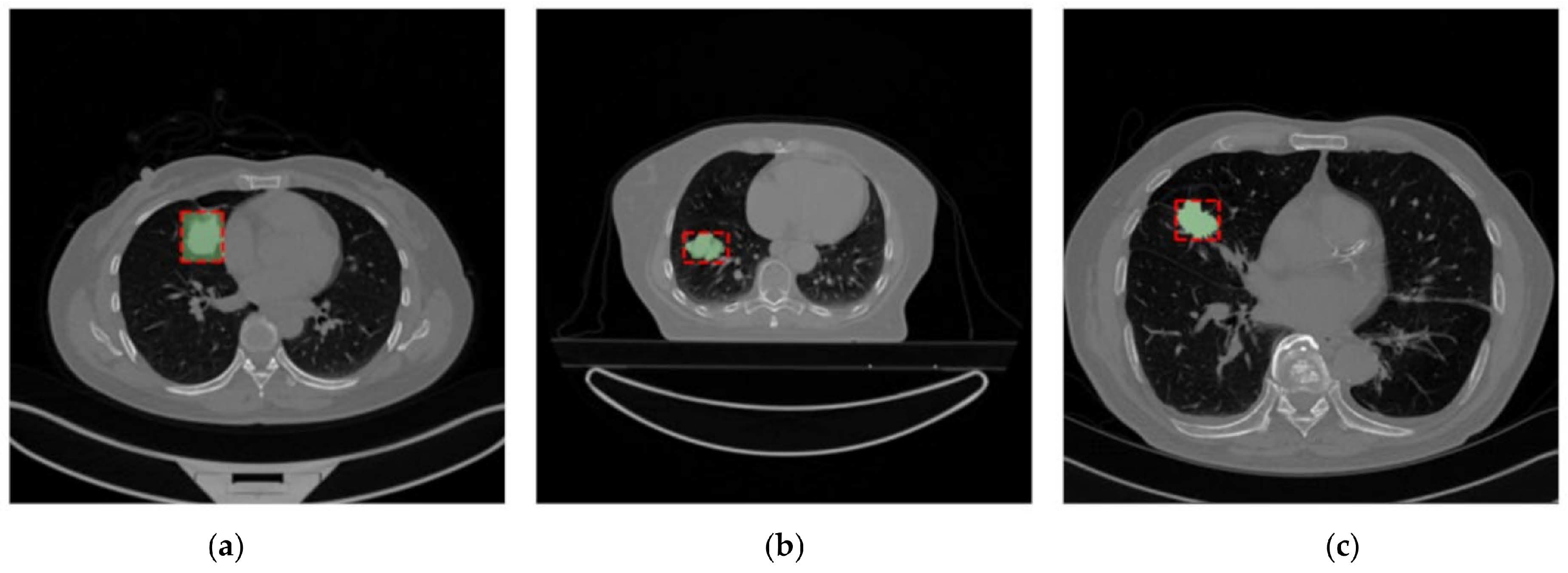
Applsci 15 01148 g001
Figure 2. Example of images from the Lung-PET-CT-Dx Dataset (a), the NSCLC-Radiomics Dataset (b), and the NSCLC-Radiogenomics (c) Dataset. The segmentations present in the dataset are shown in green and the bounding box used after the dataset uniformization is presented in red.
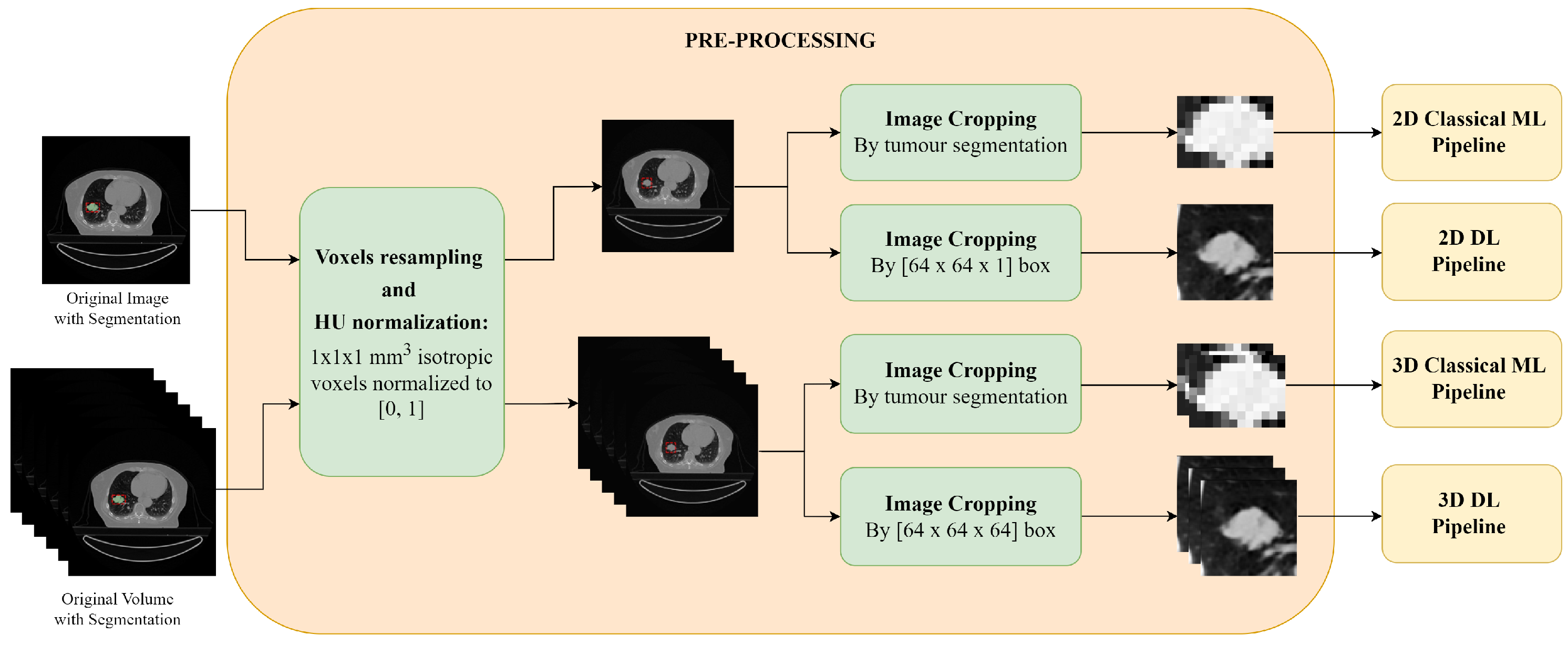
Applsci 15 01148 g002
Figure 3. Pre-processing of the 2D slices and the 3D CT scans: first a voxel resampling and discretization is applied, followed by image cropping. For the images and volumes used for the DL pipeline, image resampling and normalization are also applied.
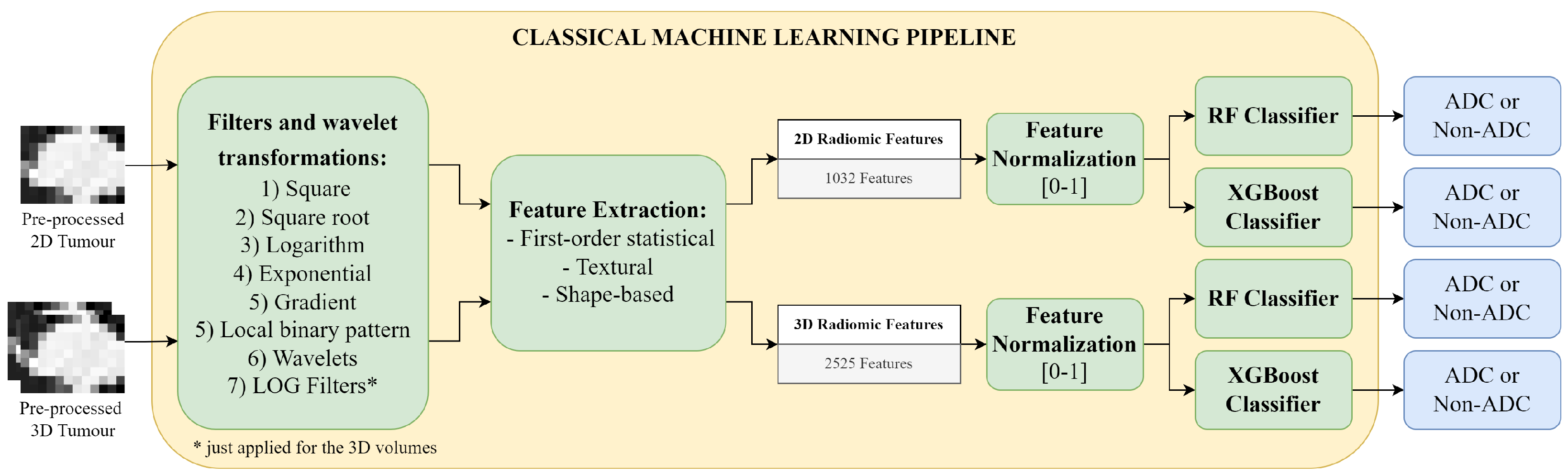
Applsci 15 01148 g003
Figure 4. Classical Machine Learning Pipeline: first several filters are applied to the 2D tumour image and the 3D tumour volume, for radiomics feature extraction; then the features are normalized and used as input to the Random Forest (RF) or the eXtreme Gradient Boosting (XGBoost) classifier for the binary classification between adenocarcinoma (ADC) and non-adenocarcinoma (Non-ADC).
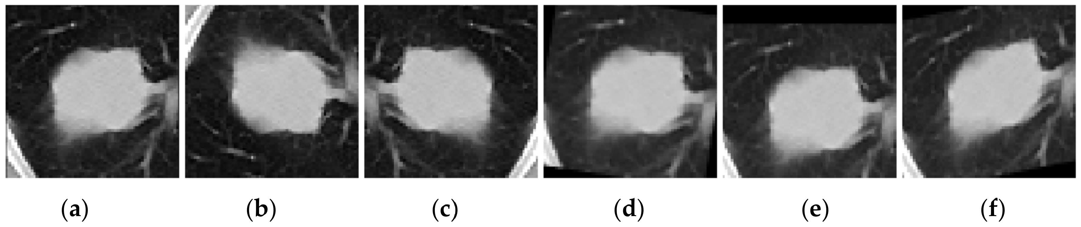
Applsci 15 01148 g004
Figure 5. Samples resulting from data augmentation transformations applied in the deep learning approach, respectively: (a) original image, (b) vertical flip, (c) horizontal flip, (d) rotation of 10°, (e) shift of 10%, and (f) shear of 10%.
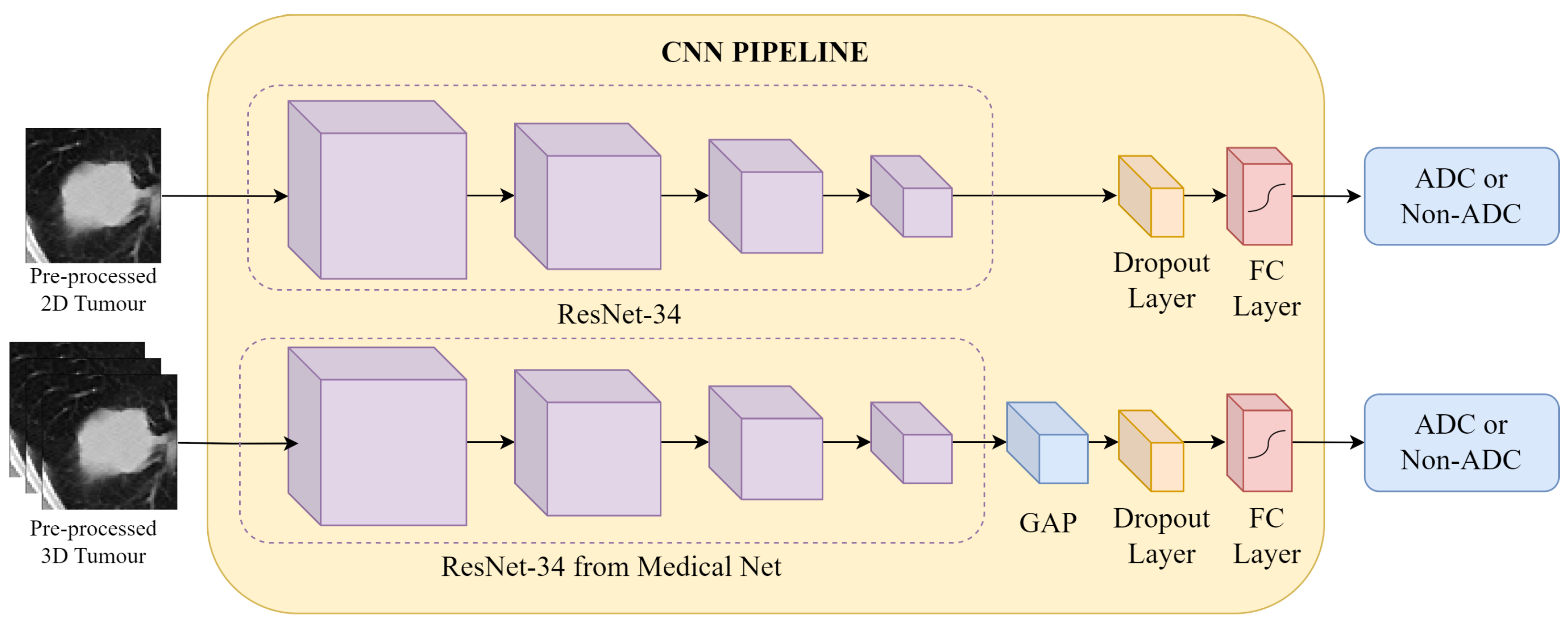
Applsci 15 01148 g005
Figure 6. CNN Pipeline: the pre-processed CT patches are fed into the respective 2D and 3D networks. In both approaches, feature extraction is conducted by a ResNet-34 architecture, followed by classification at a fully connected (FC) layer into the binary labels adenocarcinoma (ADC) and non-adenocarcinoma (Non-ADC).
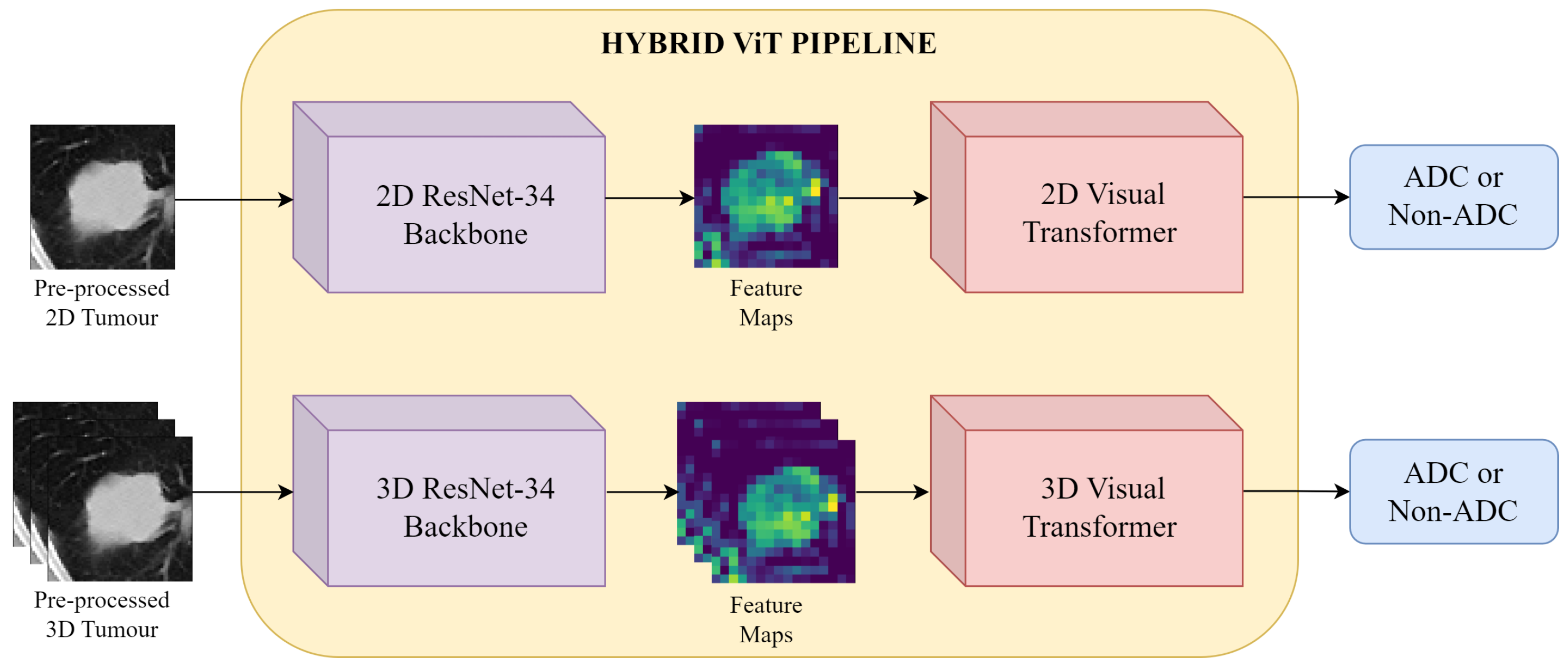
Applsci 15 01148 g006
Figure 7. Hybrid ViT Pipeline: the pre-processed CT patches are first input into the ResNet-34 backbone for feature extraction. The resulting feature maps are then fed to a ViT encoder, and finally binary classification is performed.
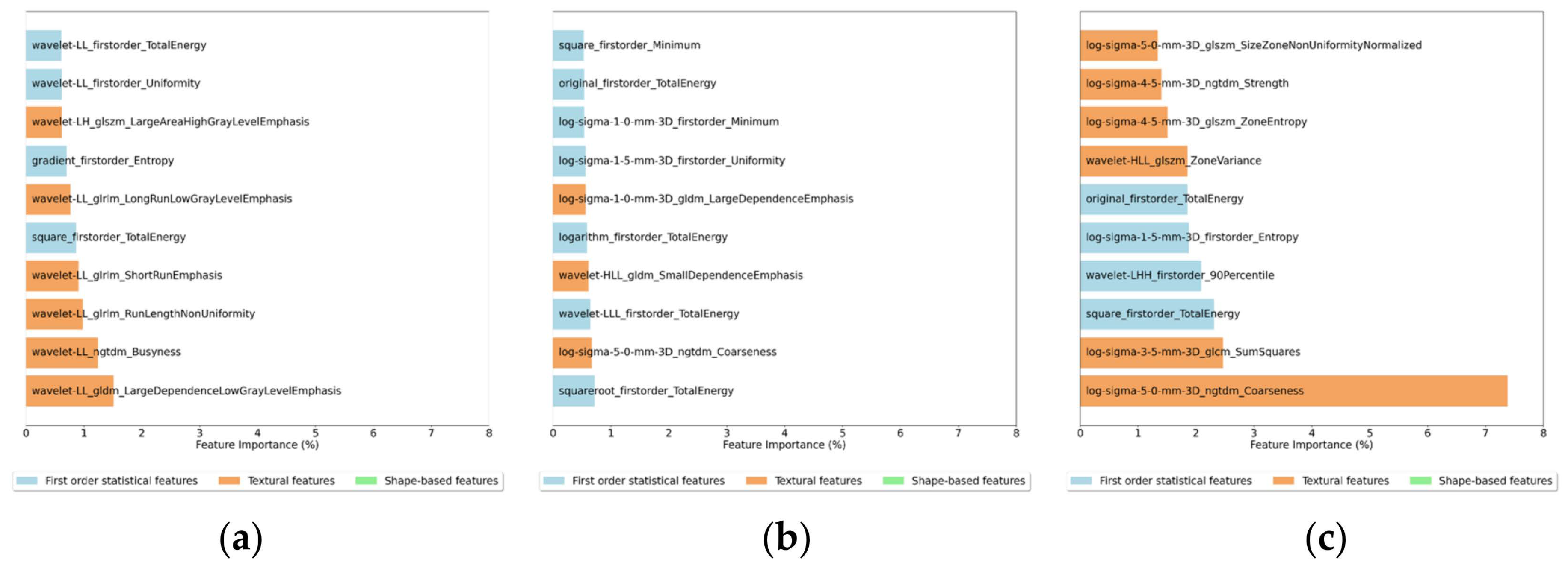
Applsci 15 01148 g007
Figure 8. Feature importance for the 10 most important features for the (a) 2D Random Forest, (b) 3D Random Forest and (c) 3D XGBoost Classifiers.
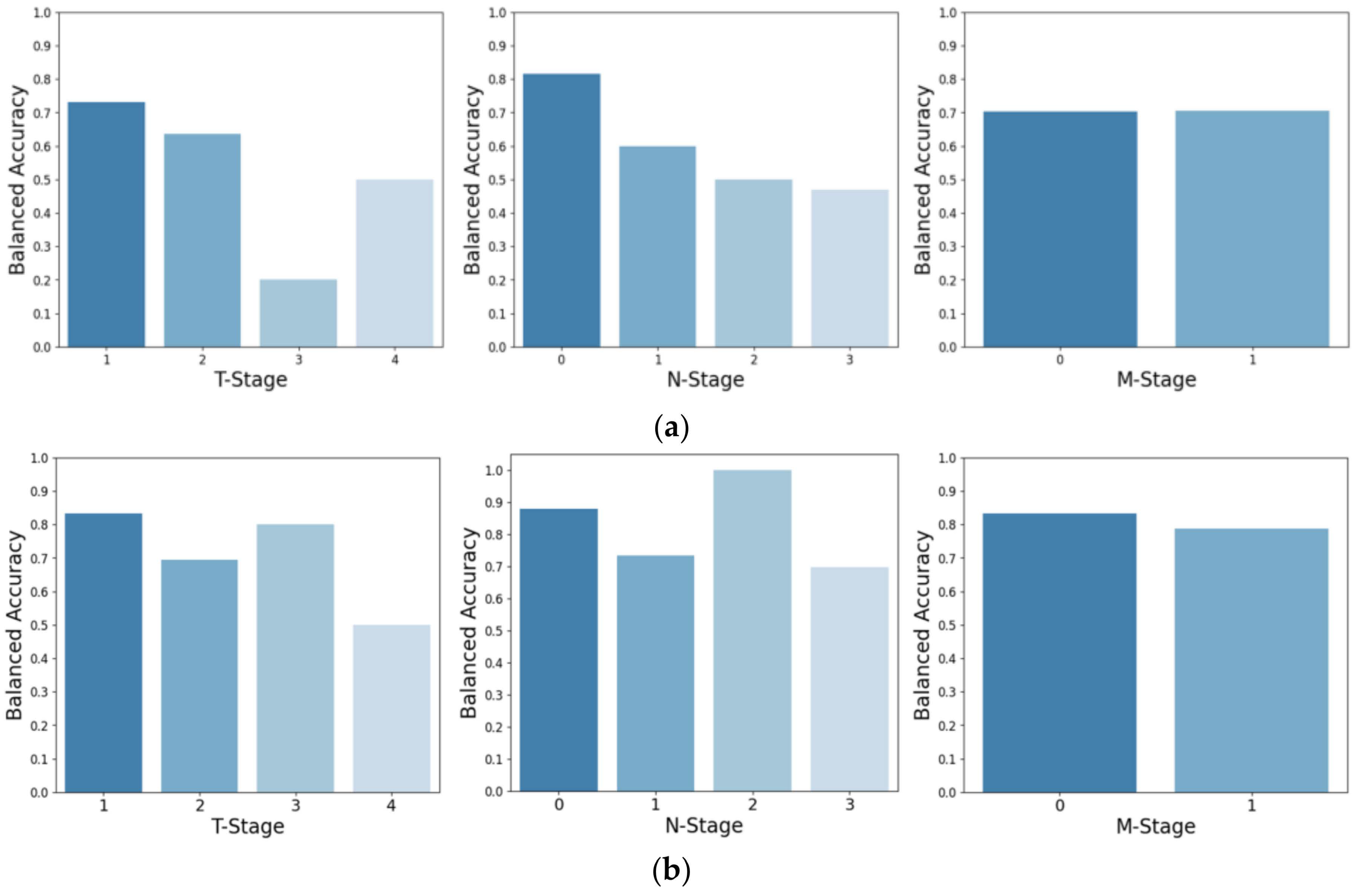
Applsci 15 01148 g008
Figure 9. Balanced accuracy based on tumour size (T-Stage), on the extent of tumour spreading (N-Stage), and metastasis state (M-Stage). The top row (a) represents the balanced accuracy for the Lung-PET-CT-Dx test set classified by the ResNet-34, while the bottom row (b) shows the corresponding results when classified by the Hybrid ViT.
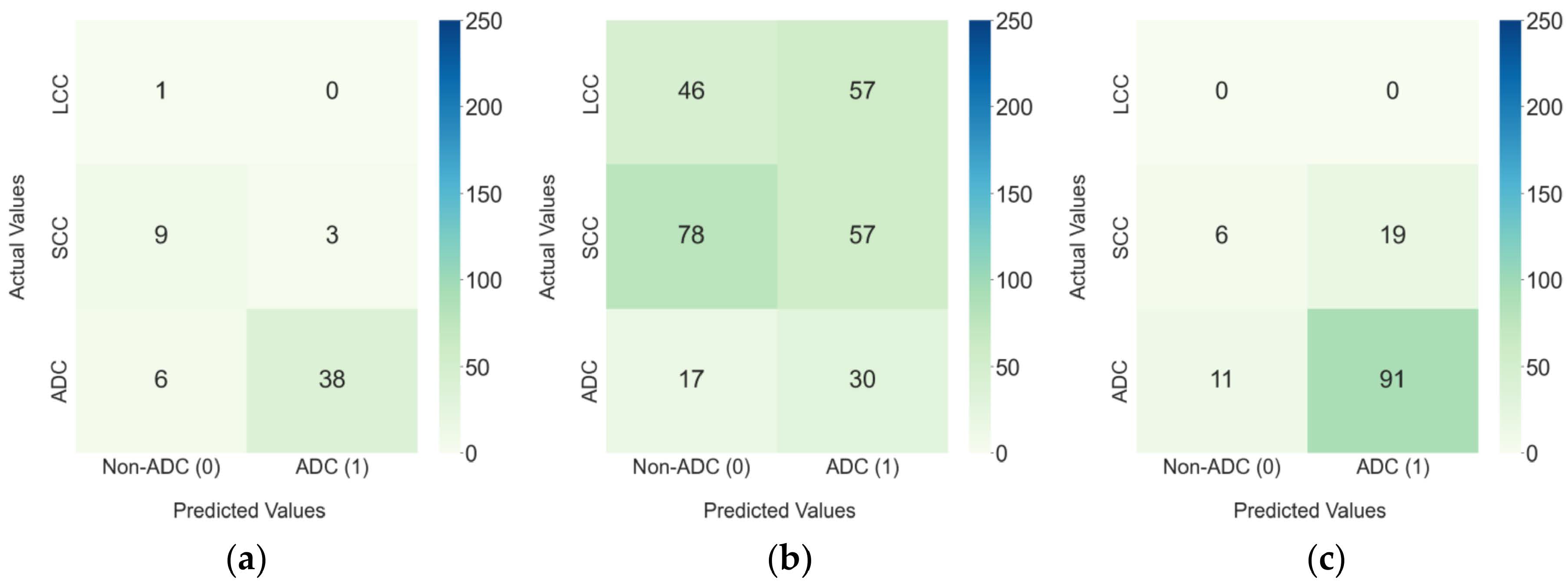
Applsci 15 01148 g009
Figure 10. Confusion matrixes for the 3D Hybrid ViT model in (a) the Lung-PET-CT-Dx internal test set and the external test sets: (b) NSCLC-Radiomics and (c) NSCLC-Radiogenomics.
Applsci 15 01148 g010
Table 1. Characterization of the final training, validation, and testing subsets, grouped by class, for the experiments performed in this work.
DatasetClassTotalTrainValidationTest
Lung-PET-CT-DxADC2211463144
Non-ADC64381313
Total2851844457
NSCLC-RadiomicsADC47--47
Non-ADC238--238
Total285--285
NSCLC-RadiogenomicsADC102--102
Non-ADC25--25
Total127--127
Table 2. Hyper-parameter values for the RF classifier.
Hyper-ParameterValues
NEstimators{50, 100, 150, 200, 250, 300, 400, 500, 750, 1000}
MaxDepth{None, 1, 10, 50, 100, 150, 200, 300}
MinSamplesSplit{2, 10, 15, 20, 25, 30, 50, 75, 100}
MinSamplesLeaf{1, 2, 4, 6, 8, 10}
Criterion{gini, entropy, log_loss}
Table 3. Hyper-parameter values for the XGBoost classifier.
Hyper-ParameterValues
NEstimators{50, 100, 150, 200, 250, 300, 400, 500, 750, 1000}
MaxDepth{None, 1, 10, 50, 100, 150, 200, 300}
MinChildWeight{1, 2, 4, 6}
η {0.001, 0.01, 0.1}
λ {0, 0.5, 1, 2}
γ {0, 0.1, 0.2, 0.3}
Table 4. Range of values defined for the parameters of the data augmentation transformations.
TransformationsRange
Flips-
Rotation[−20, 20]°
Shift[−15, 15]%
Shear[−20, 20]%
Table 5. Hyper-parameter values for the CNN.
Hyper-ParameterValues
Dropout{0, 0.5}
Learning Rate{0.000005, 0.000001, 0.00001}
Weight Decay{0, 0.001, 0.01}
Table 6. Hyper-parameter values for the Hybrid ViT.
Hyper-ParameterValues
ViT Layers{6, 8, 10}
Learning Rate{0.00001, 0.00005, 0.0001}
Weight Decay{0, 0.001, 0.01}
Table 7. Test results (AUC, balanced accuracy, precision, recall and specificity) of Random Forest and ResNet-34 on three different test sets (Lung-PET-CT-Dx, NSCLC-Radiomics, and NSCLC-Radiogenomics) for 2D and 3D input types. The highest values within each metric are highlighted in bold for each model type and test set.
ClassifierInputTest SetAUCBalanced AccuracyPrecisionRecallSpecificity
Random Forest2DLung-PET-CT-Dx0.8060.7120.8670.8860.538
NSCLC-Radiomics0.5430.4970.1640.9360.059
NSCLC-Radiogenomics0.6590.5310.8140.9410.120
3DLung-PET-CT-Dx0.8360.7620.8890.9090.615
NSCLC-Radiomics0.5600.5090.1680.8300.189
NSCLC-Radiogenomics0.6760.5550.8210.9900.120
ResNet-342DLung-PET-CT-Dx0.7830.6600.8610.7050.615
NSCLC-Radiomics0.5770.5980.2220.6380.559
NSCLC-Radiogenomics0.4950.5270.8140.8140.240
3DLung-PET-CT-Dx0.8410.7000.9550.4770.923
NSCLC-Radiomics0.5760.5500.2190.3400.761
NSCLC-Radiogenomics0.5890.5550.8390.5100.600
Table 8. Test results (AUC, balanced accuracy, precision, recall and specificity) of XGBoost and Hybrid ViT on three different test sets (Lung-PET-CT-Dx, NSCLC-Radiomics, and NSCLC-Radiogenomics) for 3D input type. The highest values within each metric are highlighted in bold for each test set.
InputClassifierTest SetAUCBalanced AccuracyPrecisionRecallSpecificity
3DXGBoostLung-PET-CT-Dx0.8530.8010.9090.9090.692
NSCLC-Radiomics0.5700.5330.1760.8720.193
NSCLC-Radiogenomics0.7450.5500.8200.9800.120
Hybrid ViTLung-PET-CT-Dx0.8690.8160.9270.8640.769
NSCLC-Radiomics0.6170.5800.2080.6380.521
NSCLC-Radiogenomics0.6130.5670.8270.8920.240
Table 9. Cumulative feature importance for each type of feature (first-order statistical, textural and shape-based features) in the (a) 2D Random Forest, (b) 3D Random Forest and (c) 3D XGBoost Classifiers.
ModelType of Features
First Order StatisticalTexturalShape-Based
2D Random Forest34.6 %64.7 %0.6 %
3D Random Forest28.3 %70.7 %0.9 %
3D XGBoost24.8 %73.8 %1.4 %
Disclaimer/Publisher’s Note: The statements, opinions and data contained in all publications are solely those of the individual author(s) and contributor(s) and not of MDPI and/or the editor(s). MDPI and/or the editor(s) disclaim responsibility for any injury to people or property resulting from any ideas, methods, instructions or products referred to in the content.

