Article

BiModalClust: Fused Data and Neighborhood Variation for Advanced K-Means Big Data Clustering

by
Ravil Mussabayev
1,*,† and
Rustam Mussabayev
1,2,†
1
AI Research Lab, Department of Software Engineering, Satbayev University, Satbayev Str. 22, Almaty 050013, Kazakhstan
2
Laboratory for Analysis and Modeling of Information Processes, Institute of Information and Computational Technologies, Pushkin Str. 125, Almaty 050010, Kazakhstan
*
Author to whom correspondence should be addressed.
These authors contributed equally to this work.
Appl. Sci. 2025, 15(3), 1032; https://doi.org/10.3390/app15031032
Submission received: 27 December 2024 / Revised: 17 January 2025 / Accepted: 18 January 2025 / Published: 21 January 2025
(This article belongs to the Section Computing and Artificial Intelligence)

Abstract

:
K-means clustering is a fundamental tool in data mining, yet its scalability and efficacy decline when faced with massive datasets. In this work, we introduce BiModalClust, a novel clustering algorithm that leverages a bimodal optimization paradigm to overcome these challenges. Our approach simultaneously optimizes two interdependent modalities: the input data stream and the neighborhood structure of the solution landscape, which emerges from iterative restrictions of the Minimum Sum-of-Squares Clustering (MSSC) objective function to sampled subsets of the data. By integrating the Variable Neighborhood Search (VNS) metaheuristic, we systematically explore and refine these landscapes through dynamic reinitialization of degenerate centroids and adaptive exploration of expanding neighborhoods. This dual-stream optimization not only transforms traditional local search into a more global and robust process but also ensures computational scalability and precision. Extensive experimentation on diverse real-world datasets demonstrates that BiModalClust achieves superior clustering performance among K-means-based methods in big data environments.

1. Introduction

Clustering is a fundamental operation in data analysis, aiming to identify cohesive groups of objects sharing similar characteristics within a given dataset. With the rapid expansion of digital information, clustering has become indispensable across a wide array of applications, such as image analysis, customer segmentation, and beyond. Among the diverse clustering paradigms, the Minimum Sum-of-Squares Clustering (MSSC) model [1] is a cornerstone methodology. MSSC seeks an optimal partitioning of m data points in a multi-dimensional space X by minimizing the total sum of squared distances between data points and their respective cluster centroids.
The mathematical formulation of MSSC is as follows:
min C f C , X = i = 1 m min j = 1 , , k | x i c j | 2
In this expression, the objective is to determine the optimal set of k centroids C such that the function f ( C , X ) —representing the sum of squared distances—is minimized. The notation | · | denotes the Euclidean norm. Each solution to this optimization problem induces a specific partitioning of the dataset into clusters, capturing inherent structure within the data.
Essentially, the primary goal of MSSC is to partition a dataset into distinct, well-defined clusters. A key characteristic of MSSC is its dual-action optimization mechanism. By minimizing the expression in Equation (1), MSSC inherently increases intra-cluster similarity while simultaneously maximizing inter-cluster dissimilarity. This balance ensures the formation of cohesive clusters that are also distinct from one another, fulfilling the core objective of clustering algorithms. Consequently, MSSC serves as both a method for generating high-quality partitions and a benchmark for evaluating clustering accuracy.
Despite its conceptual simplicity, the MSSC problem is notably challenging due to its classification as NP-hard [1]. Solving MSSC is computationally intensive, especially as data volume and dimensionality increase, underscoring the need for innovative, scalable approaches to tackle this challenge effectively. For big data scenarios [2], traditional clustering methods such as K-means and K-means++ struggle to solve the MSSC problem efficiently within a reasonable allocation of resources. This limitation creates the need for innovative techniques to tackle the big data clustering challenge.
MSSC is a global optimization problem, where the difficulty lies not only in the computational effort required but also in navigating the intricate solution landscape. The importance of identifying global minimizers in MSSC has been well-documented [3]. These minimizers provide a more faithful representation of the dataset’s intrinsic clustering patterns. However, due to the non-convex, non-smooth nature of the objective function, which becomes aggravated in big data contexts, finding global minimizers is a formidable task that often challenges conventional optimization methods.
In this work, we introduce BiModalClust, an innovative algorithm that employs a dual-modality optimization approach: (1) exploring partial solution landscapes derived from the data stream of random samples from the original dataset, and (2) iteratively traversing increasingly expansive neighborhoods within these landscapes to refine the incumbent solution. For the latter, we define a specialized neighborhood structure, where two solutions are considered neighbors if they differ in a defined subset of centroids. By strategically exploring this structure using an appropriate metaheuristic, the algorithm achieves a more informed and directed traversal of the solution space.
The simultaneous exploitation of these two modalities enables the algorithm to “shake” the incumbent solution effectively, thereby escaping unfavorable local minima. Controlling the size of input data samples allows for significant reductions in time complexity, making the algorithm inherently scalable to large datasets. Furthermore, integrating the Variable Neighborhood Search (VNS) metaheuristic [4] facilitates an in-depth exploration of each consecutive solution landscape. This enables the algorithm to address local challenges such as degenerate clusters and the fragmentation of a single true cluster into multiple centroids.
A key limitation of existing initialization-sensitive iterative methods, such as Forgy K-means and K-means++, is their inability to effectively handle scenarios where multiple initial centroids are positioned within a single well-separated cluster. This issue arises because centroids struggle to traverse the empty margins separating clusters, especially in sparsified datasets obtained through random sampling. In such cases, the centroids remain trapped, failing to converge toward an optimal solution. Section 5.3 empirically demonstrates this phenomenon and its adverse effects on clustering accuracy. By leveraging its bimodal optimization strategy, BiModalClust addresses these challenges, providing a robust and scalable solution for K-means clustering in big data contexts.
The algorithm processes the input data in a streaming fashion. During each iteration, a random sample S is drawn from the dataset X. The degenerate clusters and p randomly selected centroids from the current solution C are reinitialized using the K-means++ algorithm on the sample S. This reinitialization step acts as a “shaking” mechanism to perturb the incumbent solution and explore alternative configurations. The variable p, referred to as the shaking power, is cyclically incremented across iterations, with its upper bound defined by the hyperparameter p m a x . Following this step, a local search phase using the K-means algorithm is conducted on S, starting from the perturbed incumbent solution to identify potentially improved solutions within the current neighborhood. The iterative process continues until a predefined time limit T is reached.
Overall, this study examines the synergy between big data clustering and advanced optimization metaheuristics, particularly focusing on hybridization to enhance clustering performance. We propose a novel clustering heuristic named BiModalClust, designed to extend the global optimization capabilities of traditional clustering methods by fusing data streaming with global optimization approaches. By embedding the Variable Neighborhood Search (VNS) framework [4], a powerful metaheuristic approach, BiModalClust achieves a refined clustering methodology. Comprehensive experimental analyses conducted on a wide array of real-world datasets reveal that BiModalClust outperforms existing methods, establishing itself as the new state-of-the-art within the MSSC clustering algorithm family. Remarkably, it surpasses the current state of the art, Big-means [2], showcasing its robustness and innovative advancements in big data clustering.
The structure of this paper is as follows. Section 2 reviews related work, including existing clustering methods. Section 3 introduces the foundational concepts of the VNS metaheuristic. Section 4 presents a detailed pseudocode of BiModalClust, elaborates on its core properties, and provides an analysis of its time complexity. Section 5 outlines the experimental setup and describes the conducted experiments. Finally, Section 6 discusses the experimental results, concluding the paper with final reflections and insights.

2. Related Work

To address the high non-convexity challenge of MSSC, a variety of optimization strategies have been developed, each with unique strengths and limitations:
  • Gradient-based methods excel in quickly locating local minimizers, but their reliance on smooth gradients often leads to entrapment in suboptimal solutions due to the non-convexity of the objective function [5].
  • Stochastic optimization algorithms leverage randomness to escape local minima, enabling broader exploration of the solution space and increasing the likelihood of discovering global optima [6,7].
  • Heuristic and metaheuristic search strategies strike a balance between exploration and exploitation, systematically refining solutions while avoiding premature convergence [2,3,8].
  • Hybrid approaches, which integrate elements of gradient-based methods, stochastic algorithms, and metaheuristics, harness the complementary strengths of these techniques [9]. By synergizing their capabilities, hybrid methods often uncover superior solutions that standalone strategies might overlook.
These diverse methodologies highlight the intricate interplay of exploration and exploitation in MSSC, underscoring the need for innovative approaches to achieve effective and scalable clustering in big data environments.
The existing clustering algorithms for the MSSC problem can also be divided into two broad categories: traditional and alternative approaches.
Traditional algorithms are well-known for their simplicity and effectiveness and have been the subject of extensive research. Among these, the K-means algorithm stands out as the most widely used for solving the MSSC problem (1), along with its numerous extensions, such as Forgy [10], K-means++ [11], and multi-start K-means [12]. Another notable traditional method is Ward’s method [13], which delivers solution quality comparable to more advanced heuristics. However, a significant drawback of Ward’s method is its reliance on computing a squared distance matrix, making it impractical for large datasets due to its high computational demands.
On the other hand, alternative algorithms have been developed to overcome the limitations of traditional approaches, primarily focusing on enhancing solution quality and computational performance for the MSSC problem. Prominent examples of advanced alternative algorithms include MDEClust [9], HG-means [3], LMBM-Clust [5], I-k-means-+ [14], BWKM [15], BDCSM [16], and Coresets [17]. These methods are often characterized by their complexity and hybrid nature, incorporating meta-heuristic principles or combining simpler algorithms to enhance performance. Despite achieving the quality of a state-of-the-art solution, these alternative algorithms frequently fall short in terms of computational efficiency. In many cases, their runtime exceeds that of K-means by several orders of magnitude, making them less suitable for applications requiring rapid processing of large datasets.
Despite the significant advancements, the existing clustering methods face two fundamental challenges. First, they struggle to process big data effectively, as most algorithms require at least one complete pass through the entire dataset, which becomes infeasible when the dataset size approaches infinity. Second, they fail to ensure a thorough exploration of the intricate solution landscape, often falling into local optima traps and thereby compromising the global optimization convergence.
To address these critical issues, we propose the BiModalClust algorithm, an innovative integral clustering approach that achieves a significant leap in performance. By fusing optimization along the input data stream and the solution landscape structure modalities, our algorithm introduces qualitatively new global convergence properties while having the capacity to process big data. This dual-modal strategy not only resolves the limitations of traditional and alternative methods but also sets a new standard for robust and scalable clustering solutions.

3. Variable Neighborhood Search

3.1. Main Concepts

In the fields of computer science, artificial intelligence, and mathematical optimization, heuristics are indispensable tools for expediting problem-solving processes. They are particularly valuable when traditional methods are computationally prohibitive or when seeking exact solutions is infeasible due to the problem’s inherent complexity. It is important to note, however, that heuristics do not guarantee the discovery of the optimal solution, categorizing them as approximate algorithms. These algorithms are adept at rapidly and efficiently generating solutions that closely approximate the optimal one. In some instances, they may even achieve the exact optimal solution, but they remain classified as heuristics until their output is formally proven to be optimal [18].
Expanding on this concept, metaheuristics provide flexible and adaptive frameworks for designing heuristics, enabling them to address a wide variety of combinatorial and global optimization problems [19]. Metaheuristics generalize the heuristic approach, introducing higher-level strategies to explore the solution space more effectively and avoid pitfalls such as premature convergence to suboptimal solutions.
An optimization problem can be formally described as follows:
min f ( x ) x F X ,
where
  • X represents the ambient solution space encompassing all potential solutions,
  • F denotes the feasible subset of X where solutions satisfy predefined constraints,
  • x is an individual feasible solution within F , and
  • f is the real-valued objective function to be minimized.
In the context of MSSC (1), the feasible solution space simplifies to F = X = R n , reflecting the continuous multidimensional nature of the clustering problem.
Variable Neighborhood Search (VNS), introduced by Mladenovic in 1997 [4], is a modern metaheuristic framework that provides a flexible and robust approach to solving combinatorial and continuous nonlinear global optimization problems. The strength of VNS lies in its systematic exploitation of neighborhood changes, enabling both descent to local minima and escape from the valleys containing them [4,19,20]. This method strategically explores distant neighborhoods of the current solution and moves to a new solution only when such movement yields an improvement in the objective function.
VNS serves as a powerful tool for constructing innovative global search heuristics by integrating existing local search methods. Its effectiveness is grounded in the following foundational principles:
Fact 1:
A solution that is a local optimum under one neighborhood structure may not remain optimal when assessed using a different neighborhood.
Fact 2:
A globally optimal solution is also a local optimum for all possible neighborhood structures.
Fact 3:
For many optimization problems, local optima across one or multiple neighborhoods tend to be located in close proximity to one another.
Fact 1 establishes the basis for using diverse and complex moves to uncover local optima across multiple neighborhood structures. Fact 2 suggests that incorporating a larger variety of neighborhoods into the search process increases the likelihood of discovering a global optimum, particularly when the current local optima are suboptimal. Together, these insights propose an intriguing strategy: a solution that is a local optimum across several neighborhood structures has a higher probability of being globally optimal compared to one that is optimal within a single neighborhood [21].
Fact 3, which arises primarily from empirical observations, underscores that local optima often provide valuable insights into the characteristics of the global optimum. In essence, local optima in optimization problems tend to share structural similarities. This phenomenon highlights the utility of thoroughly exploring the neighborhoods of a given local optimum. For instance, if we aggregate all local solutions C = ( c 1 , , c k ) of the MSSC problem as defined in Equation (1) into a single set, it is likely that a significant subset of these locally optimal centroids will be clustered close to each other, while a few may deviate. This pattern suggests that the global optimum shares overlaps in certain variables (specific coordinates of the vector representations) with those found in local optima.
However, identifying these overlapping variables in advance is inherently difficult. Consequently, a methodical exploration of neighborhoods surrounding the current local optimum remains prudent, continuing until a superior solution emerges. This systematic neighborhood search not only enhances the likelihood of escaping suboptimal solutions but also leverages the structural tendencies of the problem to converge more efficiently toward the global optimum.
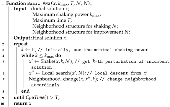
Variable Neighborhood Search (VNS) operates through two fundamental phases: the improvement phase, which refines the current solution by descending to the nearest local optimum, and the shaking (or perturbation) phase, which seeks to escape local minima traps. These phases are alternated with a neighborhood change step, and the process repeats until predefined stopping criteria are satisfied. The VNS framework revolves around three primary, iterative steps:
  • a shaking procedure, which introduces a controlled perturbation to the current solution to explore new areas of the solution space;
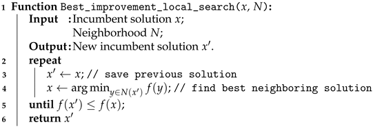
  • an improvement procedure, which applies local search techniques to refine the perturbed solution, potentially reaching a local optimum;
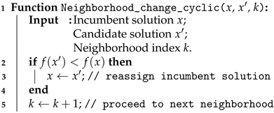
  • a neighborhood change step, which alters the neighborhood structure, allowing exploration of different regions of the solution space.
To better understand the VNS framework, let us define some essential concepts:
The incumbent solution is the current best-known solution, denoted as x, which minimizes the objective function value among all solutions examined thus far.
For a given solution x, its neighborhood comprises the set of solutions that can be directly obtained from x by applying a specific local change. Neighborhoods are typically defined using a metric (or quasi-metric) function, denoted as δ . For a non-negative distance threshold Δ 0 , the neighborhood of x is formally defined as
N Δ ( x ) = y F δ ( x , y ) Δ
Examples of neighborhoods:
  • In continuous optimization problems over R n , a neighborhood like N 1 ( x ) might represent an Euclidean ball of radius 1 centered at x, while N 3 ( x ) could include solutions obtained by modifying exactly three coordinates of x.
  • In the Traveling Salesman Problem (TSP), a common neighborhood involves all tours generated by reversing a subsequence of the current tour, an operation known as the “2-opt” move.
Neighborhoods play a critical role in both the shaking and improvement phases, enabling VNS to effectively explore the solution space and navigate complex optimization landscapes. By iteratively combining these steps, VNS achieves a balance between diversification (escaping local optima) and intensification (refining toward better solutions), making it a powerful tool for solving global optimization problems.
A neighborhood structure, denoted as N , is defined as an ordered collection of operators:
N = { N 1 , , N k max } ,
where each operator N k : F P ( F ) maps a solution x F to a predefined set of neighboring solutions N k ( x ) within the feasible solution space F . Here, P ( F ) represents the power set of F , and k 1 , , k max indexes the individual neighborhoods. This hierarchical arrangement of neighborhoods is a cornerstone of the VNS framework. When local search within one neighborhood fails to uncover an improved solution, the algorithm systematically transitions to the next neighborhood in the sequence, thereby expanding the search scope and increasing the likelihood of finding superior solutions. By dynamically adjusting the neighborhood structures during the search process, VNS can effectively navigate complex solution landscapes and escape local optima. Throughout this discussion, the terms “neighborhood structure” and “neighborhood” are used interchangeably to refer to both the collection of operators N and the set of neighborhoods N ( x ) associated with a given solution x.
Each neighborhood structure employs a unique method to define the relationship between a solution and its neighbors. For example, in the context of the Traveling Salesman Problem (TSP), a neighborhood structure can be constructed using “k-opt” moves. In this case, k edges are removed from the current tour, and the resulting segments are reconnected in a new configuration to generate alternative solutions.
To distinguish between the neighborhood structures used in different phases of the VNS algorithm, we introduce two separate notations: N is reserved for the neighborhood structures utilized during the shaking phase, which introduces perturbations to the incumbent solution, while N is used for the neighborhoods explored during the improvement phase, where local search is conducted to refine the solution. This distinction ensures clarity and emphasizes the complementary roles of shaking and local search in the VNS process.

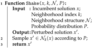
3.2. The Shaking Procedure

The shaking procedure is a critical step in the VNS framework, designed to help the algorithm escape local optima traps by introducing controlled perturbations to the current solution.
The simplest form of a shaking procedure involves randomly selecting a solution from the neighborhood N k ( x ) , where k, the shaking power, is a predetermined index that defines the scope of the neighborhood. The shaking power k determines the degree of perturbation applied to the current solution during the shaking step. It controls how far the algorithm explores the search space by systematically increasing the “intensity” or “distance” of the perturbation.
While effective in many cases, a purely random jump within the k-th neighborhood can occasionally result in excessively aggressive perturbations, particularly for problems where the objective function is highly sensitive to changes in the solution. To address this, alternative approaches such as intensified shaking may be employed, where the perturbation considers the sensitivity of the objective function to small variations in the decision variables. Such methods allow for more focused and deliberate perturbations.
However, for the purposes of this work, we adopt a straightforward random-selection shaking approach, which is both effective and computationally efficient. In this method, the next solution is chosen at random from the k-th neighborhood N k ( x ) based on a predefined probability distribution. This ensures sufficient exploration of the solution space while maintaining simplicity. The pseudocode for this procedure is presented in Algorithm 1.
Algorithm 1: Shaking Procedure
Applsci 15 01032 i001

3.3. Neighborhood Change Step

The neighborhood change procedure plays a pivotal role in guiding the Variable Neighborhood Search (VNS) heuristic through the solution space. It determines both the sequence of neighborhoods to explore and whether a candidate solution should replace the incumbent. Different strategies for neighborhood change have been explored in the literature [21], with the sequential and cyclic methods being the most commonly employed.
  • In the sequential approach, the search systematically navigates through the neighborhoods, restarting at the first neighborhood in the structure whenever an improvement to the incumbent solution is found. If no improvement occurs, the search progresses to the next neighborhood in the sequence. This strategy ensures that the search refocuses on promising areas of the solution space after discovering a better solution.
    The sequential neighborhood change procedure is outlined in Algorithm 2:
    Algorithm 2:  Sequential Neighborhood Change Step
    Applsci 15 01032 i002
  • In the cyclic approach, the search moves to the next neighborhood regardless of whether an improvement in the incumbent solution occurs. This method maintains a consistent exploration cycle through all neighborhoods, avoiding overcommitment to any single region of the solution space.
    The cyclic neighborhood change procedure is described in Algorithm 3:
    Algorithm 3: Cyclic Neigborhood Change Step
    Applsci 15 01032 i003

3.4. The Improvement Procedure

The local search heuristic represents a fundamental and widely used approach for solution improvement [21]. It iteratively explores the neighborhood structure N ( x ) of the incumbent solution x. The process begins with the incumbent solution and systematically evaluates its neighborhood. If a superior solution is identified within N ( x ) , this solution replaces the incumbent. This iterative improvement continues until a locally optimal solution is reached, where no further improvements are possible within the neighborhood.
Two common strategies are employed to traverse the neighborhood N ( x ) :
  • The first improvement search immediately adopts the first encountered solution in N ( x ) that offers an improvement over the incumbent. This approach is faster and often suitable for large neighborhoods or problems requiring quick decisions.
  • The best improvement search evaluates all potential solutions in N ( x ) and selects the best among them as the new incumbent. While computationally more expensive, this method ensures a more comprehensive exploration of the neighborhood, often yielding higher-quality solutions.
For the purposes of this work, we focus on the best improvement strategy due to its effectiveness in identifying high-quality local optima. The pseudocode for this approach is provided in Algorithm 4.
Algorithm 4: Local Search Using Best Improvement
Applsci 15 01032 i004

3.5. Basic Variable Neighborhood Search

Unlike many other metaheuristic frameworks, Variable Neighborhood Search (VNS) and its extensions stand out for their inherent simplicity. They often require minimal or no parameter tuning, making them accessible and straightforward to implement. This simplicity does not come at the expense of performance—VNS frequently delivers high-quality solutions more efficiently than alternative methods. Moreover, its transparent structure offers valuable insights into the mechanisms that drive its effectiveness. These insights can inform the design of more refined and efficient implementations, further advancing its applicability [19].
The pseudocode for the basic VNS algorithm is provided in Algorithm 5.
Algorithm 5: Basic Variable Neighborhood Search
Applsci 15 01032 i005
Within the basic Variable Neighborhood Search (VNS) framework, the following key components are integral to its operation:
  • f ( x ) : The real-valued objective function to be minimized or maximized.
  • k: The current shaking intensity, which determines the scale of the perturbation applied to the incumbent solution.
  • k max : The maximum shaking intensity, defining the upper limit for neighborhood exploration during the shaking phase.
  • N k ( x ) : The k-th neighborhood of the incumbent solution x, representing a set of candidate solutions generated by applying perturbations of intensity k.
  • x: The incumbent solution, representing the best-known solution at a given point in the search.
  • x Shake ( x , k , N ) : A procedure (detailed in Section 3.2) that generates a candidate solution x by randomly selecting a solution from the k-th neighborhood N k ( x ) of the incumbent solution x.
  • N e i g h b o r h o o d _ C h a n g e ( x , x , k ) : A mechanism (described in Section 3.3) for adapting the neighborhood structure based on the current solution and the search’s progress. Usually, either Algorithm 2 or Algorithm 3 can be used for this process.
  • x L o c a l _ S e a r c h ( x , N ) : A local search procedure (outlined in Section 3.4) that explores the vicinity of the candidate solution x to locate a locally optimal solution, x . Usually, Algorithm 4 is used for this purpose.
  • CpuTime ( ) : A function that returns the elapsed time since the algorithm’s initiation, ensuring adherence to the predefined time constraints.
  • T: A predefined, relatively short time limit for the search, serving as a stopping criterion to prevent excessive computation.

4. The Proposed Algorithm

This section presents a mathematically precise description of the proposed BiModalClust algorithm, accompanied by an in-depth analysis of its internal mechanisms and time complexity.

4.1. Precise Description

The pseudocode for the proposed BiModalClust algorithm is presented in Algorithm 6. In the context of the Minimum Sum-of-Squares Clustering (MSSC) problem, where k conventionally denotes the number of clusters, we adopt the variables p and p max to represent the current and maximum shaking powers, respectively. This distinction ensures clarity in the algorithm’s parameterization while maintaining consistency with the MSSC notation.
The proposed Algorithm 6 builds upon the basic VNS framework outlined in Algorithm 5, incorporating the following components:
  • The neighborhood structure N utilized in the shaking phase is defined as follows:
    • Let S X be a uniform random sample of size s from X.
    • Let U = ( u 1 , , u l ) R l × n represent a finite subset of points in X.
    • Define a probability distribution P : X [ 0 ,   1 ] by
      P U ( x ) = d ( x , U ) x X d ( x , U )
      where d ( x , U ) denotes the distance from a point x to the set U. This distribution corresponds to the one used in K-means++ initialization.
    Let C = ( c 1 , , c k ) denote the incumbent solution. Adopting the notation N k = { 1 , , k } , the p-th neighborhood N p ( C ) of the incumbent solution is then defined as
    N p ( C ) = { ( c 1 , c 2 , , c l 1 , , c l 2 , , c l p , , c k ) | where l 1 < l 2 < < l p N k such that l i l j for i j , and for every i N p , U i = { c j } j N k , j { l i , , l p } , c l i S U i is sampled according to P U i } ;
Algorithm 6: Dual-Modality Optimization Approach for Big Data Clustering
Applsci 15 01032 i006
2.
The local search procedure is based on Algorithm 4. The neighborhood structure N ( C ) for the incumbent solution C is defined as
N ( C ) = i N k Conv ( S i ) ,
where S i S , i N k , represents the set of all sample points assigned to cluster c i , i.e.,
S i = { x S | arg min c C d ( x , c ) = c i } ,
and Conv ( · ) denotes the convex hull operation.
Searching within the convex hull of the sample points in each cluster is justified by a key property of the squared Euclidean distance function:
  • The optimal placement of the centroid (to minimize the sum of squared distances) is always within the convex hull of its assigned points.
  • As the centroid approaches the mean of the assigned points, the sum of squared Euclidean distances decreases, reaching its minimum when the centroid coincides with the mean of the points [22].
Thus, the K-means algorithm is employed for local search due to its reliance on these fundamental properties.
3.
The neighborhood change follows Algorithm 3. In each iteration, the shaking power p is incremented, regardless of whether the objective function has improved or not.
Empirical studies have demonstrated that the specific combination of VNS components described above is critical to achieving the best performance of BiModalClust, both in terms of computational efficiency and the quality of the solutions obtained.
It is important to highlight that BiModalClust does not strictly conform to the traditional VNS metaheuristic. Unlike standard VNS, both the neighborhood structure N used in the shaking phase and the local search procedure operate on a sample S, rather than the entire dataset X. Despite this deviation, the approach aligns with the newly introduced Variable Landscape Search (VLS) metaheuristic, as detailed in [23], under which BiModalClust is formally categorized.

4.2. Analysis of the Algorithm

The proposed algorithm, BiModalClust, iteratively constructs and optimizes partial solution landscapes for the MSSC problem, restricted to relatively small input data samples S that are randomly drawn from the original dataset X. The K-means algorithm serves as the local search mechanism, identifying optimal solutions within cyclically expanding neighborhoods of the incumbent solution C.
BiModalClust also incorporates an explicit shaking procedure to perturb the incumbent solution. Following the local search phase, exactly p random centroids, including any degenerate ones, are reinitialized within the incumbent solution C. As p increases, the intensity of the perturbation applied to C grows. In the extreme case where p max = k and p reaches p max , the entire incumbent solution is reinitialized using the K-means++ seeding strategy. This results in a complete restart of the solution. However, it is generally more practical to set p max to a value much smaller than k. Limiting p max ensures that the applied perturbations remain controlled, preventing a total or near-total restart.
The shaking power p is incrementally increased with each iteration. This approach allows for a gradual yet controlled expansion of the search space for the local search procedure in each successive partial solution landscape. By leveraging the K-means++ seeding logic to sample new centroids during the shaking phase, BiModalClust ensures that the newly introduced centroids are well-distributed across the sample, promoting optimal coverage. This strategy minimizes the risk of the incumbent solution becoming trapped in local minima, such as scenarios where multiple cluster centers are positioned too closely together, erroneously splitting a single true cluster.

4.3. Time Complexity

In Algorithm 6, the time complexity for the K-means++ reinitialization of p centroids and any degenerate clusters (as detailed in Line 10) matches that of a single iteration of the K-means local search, which is O ( s · n · k ) . This equivalence holds because both operations are conducted on a sample S of size s.
The additional process described in Lines 18–20 of Algorithm 6, responsible for incrementing the shaking power p, has a constant time complexity of O ( 1 ) . Therefore, the overall computational complexity of one iteration of the BiModalClust algorithm is O ( s · n · k ) , maintaining parity with the complexity of Big-means algorithm.

5. Experimental Evaluation

This section describes the experiments: the hardware and software, the selection of competitive algorithms, datasets, the experimental design and evaluation metrics, the hyperparameter selection strategy, the reproducibility package, and the numerical results of the main and synthetic experiments.

5.1. Main Experiment Settings

The experiments were carried out on a system running Ubuntu 22.04 64-bit, equipped with an AMD EPYC 7663 processor featuring 8 active cores and 1.46 TB of RAM (Santa Clara, CA, USA). The software environment comprised Python 3.10.11, NumPy 1.24.3, and Numba 0.57.0. To accelerate Python code execution and enable parallel processing, we leveraged Numba [24]. By compiling Python code into optimized machine code and distributing computations across multiple processors, Numba proved instrumental in enhancing the performance and efficiency of our experiments.
A comprehensive experimental analysis was conducted to evaluate the improvements brought by BiModalClust compared to the state-of-the-art Big-means algorithm [2]. The Big-means algorithm has already been compared with other existing clustering approaches, so it only suffices to show that BiModalClust surpasses Big-means. Additionally, we only include K-means++ as a baseline. To ensure a fair and consistent comparison, both algorithms were tested under identical conditions, utilizing the inner parallelization technique proposed in [25,26]. Exploring optimal parallelization strategies specifically tailored for the BiModalClust algorithm remains an open avenue for future research.
The experimental evaluation was conducted on 19 publicly available datasets, with 4 of them additionally normalized to enhance the results. This brings the total number of datasets to 23. These datasets are identical to those used in [2]. Table 1 provides a detailed description of the datasets, including the number of samples and features. Additionally, Table 2 lists the corresponding download links for the datasets. All datasets are numerical, are free of missing values, and demonstrate considerable diversity in size (ranging from 7797 to 10,500,000 instances) and the number of attributes (spanning from 2 to 5000). This variability enabled us to assess BiModalClust’s adaptability to a wide range of data scales. Additionally, we adopted the methodology outlined by Karmitsa et al. [5] to ensure a consistent framework for comparative analysis.
Clustering experiments were conducted on each dataset n e x e c times, varying the number of clusters (k) across the values 2, 3, 5, 10, 15, 20, and 25. Each clustering execution was treated as an independent experiment. The performance of each experiment was evaluated using two metrics: the relative error ( ε ) and CPU time (t). The relative error measures the deviation of the algorithm’s result (f) from the historical best-known result ( f * ) using the formula ε = 100 · ( f f * ) / f * . A negative relative error indicates that the algorithm surpassed the best-known performance.
The experimental results are presented in a customized table format. For each combination of dataset (X) and cluster count (k), n e x e c clustering experiments were performed, resulting in a set of outcomes. Within each set, we calculated the minimum, median, and maximum values for both the relative error ( ε ) and the CPU time (t). To provide an overall view, the results were averaged across multiple runs, and the tables display the aggregated metrics for each dataset across all k values. Table 3 and Table 4 offer a comparative analysis of BiModalClust and Big-means.
For example, consider a table entry for a specific algorithm and dataset: ISOLET #Succ = 6/7; Min = 0.01; Median = 0.24; Max = 0.59. This indicates that clustering was executed for 7 different cluster numbers (k = 2, 3, 5, 10, 15, 20, and 25), with 15 independent runs conducted for each combination of dataset and cluster number. Thus, a total of 7 sets of experiments were performed, each containing 15 results. The value “#Succ = 6/7” indicates that, for 6 out of the 7 cluster configurations, the algorithm’s median performance exceeded the median performance of all other algorithms.
The tables’ final rows summarize the overall performance of each algorithm across all datasets. To highlight top-performing results, the best metrics for each dataset and cluster configuration are bolded. An algorithm is considered successful if its median performance for a given cluster number (k) equals or surpasses the best result among all algorithms for that configuration.
The K-means clustering process was constrained by a CPU time limit (T) and terminated under specific conditions: if it exceeded 300 iterations or if the improvement between consecutive steps was less than 0.0001. For the K-means++ initialization, we selected three candidate points for each centroid to enhance seeding efficiency. Sample sizes were fine-tuned through preliminary tests to achieve optimal performance.
The reproducibility package for the BiModalClust algorithm, including implementations of various parallel strategies, is available at https://github.com/rmusab/bi-modal-clust (accessed on 17 January 2025).

5.2. Main Experiment Results

A total of 7366 experiments were conducted in our study.
Our analysis revealed no strong correlation between the choice of neighborhood change procedure and the results obtained. However, the cyclic neighborhood change procedure demonstrated a slight advantage over the sequential approach, yielding marginally better final accuracy.
Additionally, we investigated two distinct strategies for centroid shaking within the algorithm: a uniformly random approach and reinitialization based on the K-means++ method. While the uniformly random strategy offered faster execution, it significantly compromised final accuracy, with accuracy deteriorating by as much as fivefold compared to K-means++ reinitialization. This performance gap can be attributed to the uniformly random method introducing excessive perturbation to the incumbent solution. Such drastic changes require substantially more iterations during the local search phase to reach an optimal solution, thereby reducing overall efficiency.
For each algorithm, dataset (X), and cluster count (k), the minimum, median, and maximum values of relative error ( ε ) and CPU time (t) were computed over n e x e c runs. To determine the optimal maximum shaking power ( p max ), additional experiments were performed by restarting the algorithm with varying p max values according to the line search parameter optimization strategy.
Line search optimization demonstrated that increasing the intensity of shaking generally leads to improved accuracy, albeit with a slight increase in the maximum convergence time. The optimal value of p max , based on median relative accuracy, was found to be 4. These findings suggest that more vigorous shaking enhances the algorithm’s ability to escape local minima by effectively “jumping out” of their valleys. However, as expected, the subsequent descent from these perturbed positions via local search requires additional computational time.
The overall performance of BiModalClust with the best-performing configuration ( p max = 4 ) is summarized in Table 3 and Table 4.
In Table 3, it can be observed that BiModalClust achieves average relative error results that are more than 3.3 and 6.5 times better than those of Big-means and K-means++, respectively. This performance gain is attributed to the enhanced fluidity of centroids, achieved by fusing random sample data streaming with systematic neighborhood exploration.
As can be seen in Table 4, while BiModalClust demonstrates slightly longer processing times than Big-means, its computational efficiency remains competitive, with average runtime results under 3.0 s, outperforming advanced parallel HPClust variants from [25,26]. The baseline K-means++ algorithm falls far behind in efficiency due to its inability to process big datasets.
The observed efficiency of BiModalClust, coupled with its significant accuracy improvements, positions BiModalClust as a powerful and practical tool for solving industry-level big data clustering problems.

5.3. Synthetic Experiment Results

In each iteration of BiModalClust, the sampling process introduces a level of sparsification to the dataset. This sparsification allows the initial centroids to move more freely between overlapping clusters, enhancing their flexibility within the current solution. By carefully selecting an appropriate sample size, the algorithm maintains a balance between enabling centroid flexibility and preserving a reasonable approximation of the original dataset. Striking this balance is critical for achieving effective clustering results.
To further investigate this hypothesis, additional experiments were conducted using synthetic data.
Consider a mixture of three isotropic Gaussian distributions { N 1 , N 2 , N 3 } with standard deviations 0.15 , 0.08 , 0.1 , respectively. The mean coordinates of these distributions are μ 1 = [ 0.2 , 0.5 ] T , μ 2 = [ 0.7 , 0.8 ] T , μ 3 = [ 0.5 , 1.0 ] T . The dataset X 1 was generated by sampling 3000 points from N 1 , 1500 points from N 3 , and 1500 points from N 3 . The resulting dataset X 1 is visualized in Figure 1a.
Now, consider the initial centroids C = { c 1 , c 2 , c 3 } assigned as c 1 = [ 0.1 , 0.2 ] T , c 2 = [ 0.1 , 0.15 ] T , c 3 = [ 0.5 , 1.0 ] T . Running K-means++ on X 1 with these initial centroids results in the clustering shown in Figure 1b. The objective function value for the ground truth centroids is f ( { μ 1 , μ 2 , μ 3 } , X 1 ) = 171.5 . However, K-means++ converges to a suboptimal local minimum with an objective value of 191.52 , indicating that it failed to escape a poor solution.
Using BiModalClust with a sample size of s = 70 and a time limit of T = 1.5 , the algorithm achieves the clustering shown in Figure 1c, with an objective function value of 172.08 . This demonstrates that BiModalClust successfully avoided being trapped in a poor local minimum, highlighting its ability to overcome limitations inherent in K-means++.

6. Conclusions and Future Research

The summarized experimental results highlight the transformative impact of BiModalClust, a novel bimodal clustering algorithm, which significantly enhances clustering accuracy by leveraging a unique dual-modality optimization strategy. By simultaneously optimizing across two interdependent problem modalities—the input data stream and the neighborhood structures of the solution landscape stream—BiModalClust achieves a level of flexibility and robustness unattainable by traditional methods like Big-means. This bimodal approach enables the algorithm to iteratively refine the MSSC objective function on restricted data samples while dynamically exploring expanding neighborhoods of the incumbent solution, leading to superior clustering performance.
The integration of the VNS metaheuristic further strengthens this bimodal framework. VNS introduces a sophisticated shaking mechanism that systematically perturbs the incumbent solution by reassigning centroids, facilitating an intensive exploration of the solution landscape. This iterative shaking, combined with the algorithm’s natural adaptability to sparse data samples, empowers BiModalClust to effectively escape local minima and navigate complex clustering scenarios. By allowing centroids from distinct, non-overlapping clusters to traverse and realign dynamically, the algorithm avoids common pitfalls such as centroid overlap within well-separated clusters—a limitation often observed in simpler methods like Big-means.
The conceptual strength of BiModalClust lies in its ability to harness the synergy between data-driven optimization and neighborhood-based exploration. This fusion of input data sampling and systematic neighborhood variation represents a paradigm shift in big data clustering. Unlike HPClust approaches, which rely on parallel configurations to mitigate centroid initialization issues, BiModalClust naturally resolves these challenges through its bimodal mechanism. By optimizing across both the data and neighborhood modalities, it not only achieves better accuracy but also ensures a more balanced exploration–exploitation tradeoff, making it uniquely capable of addressing the demands of large-scale clustering tasks.
The lack of an efficient parallelization scheme tailored to the BiModalClust framework can be considered as its main limitation. Thus, future research exploring advanced parallelization strategies tailored to the proposed bimodal framework could further amplify performance and scalability. Also, future research directions could involve extending the algorithm beyond the MSSC formulation to encompass other clustering paradigms. Additionally, exploring the integration of other established metaheuristics holds potential for further enhancing the performance of Big-means, potentially achieving even greater improvements.

Author Contributions

Conceptualization, R.M. (Ravil Mussabayev); Methodology, R.M. (Rustam Mussabayev); Software, R.M. (Ravil Mussabayev); Validation, R.M. (Ravil Mussabayev); Formal analysis, R.M. (Ravil Mussabayev); Investigation, R.M. (Ravil Mussabayev); Resources, R.M. (Rustam Mussabayev); Data curation, R.M. (Rustam Mussabayev); Writing—original draft, R.M. (Ravil Mussabayev); Writing—review & editing, R.M. (Rustam Mussabayev); Visualization, R.M. (Ravil Mussabayev); Supervision, R.M. (Rustam Mussabayev); Project administration, R.M. (Rustam Mussabayev); Funding acquisition, R.M. (Rustam Mussabayev). All authors have read and agreed to the published version of the manuscript.

Funding

This research was funded by the Science Committee of the Ministry of Science and Higher Education of the Republic of Kazakhstan (grant no. BR21882268).

Data Availability Statement

The data presented in this study are openly available in UCI Machine Learning Repository and are listed in the published article with the following DOI: https://doi.org/10.1016/j.patcog.2022.109269. UCI Machine Learning Repository [https://archive.ics.uci.edu/] accessed on 17 January 2025.

Conflicts of Interest

The authors declare no conflicts of interest.

References

  1. Aloise, D.; Deshpande, A.; Hansen, P.; Popat, P. NP-hardness of Euclidean sum-of-squares clustering. Mach. Learn. 2009, 75, 245–248. [Google Scholar] [CrossRef]
  2. Mussabayev, R.; Mladenovic, N.; Jarboui, B.; Mussabayev, R. How to Use K-means for Big Data Clustering? Pattern Recognit. 2023, 137, 109269. [Google Scholar] [CrossRef]
  3. Gribel, D.; Vidal, T. HG-means: A scalable hybrid genetic algorithm for minimum sum-of-squares clustering. Pattern Recognit. 2019, 88, 569–583. [Google Scholar] [CrossRef]
  4. Mladenovic, N.; Hansen, P. Variable neighborhood search. Comput. Oper. Res. 1997, 24, 1097–1100. [Google Scholar] [CrossRef]
  5. Karmitsa, N.; Bagirov, A.M.; Taheri, S. Clustering in large data sets with the limited memory bundle method. Pattern Recognit. 2018, 83, 245–259. [Google Scholar] [CrossRef]
  6. Mussabayev, R.; Mussabayev, R. Comparative Analysis of Optimization Strategies for K-means Clustering in Big Data Contexts: A Review. arXiv 2024, arXiv:2310.09819. [Google Scholar]
  7. Mussabayev, R.; Mussabayev, R. Superior Parallel Big Data Clustering Through Competitive Stochastic Sample Size Optimization in Big-Means. In Intelligent Information and Database Systems; Nguyen, N.T., Chbeir, R., Manolopoulos, Y., Fujita, H., Hong, T.P., Nguyen, L.M., Wojtkiewicz, K., Eds.; Springer: Singapore, 2024; pp. 224–236. [Google Scholar] [CrossRef]
  8. Hansen, P.; Mladenovic, N. J-Means: A new local search heuristic for minimum sum of squares clustering. Pattern Recognit. 2001, 34, 405–413. [Google Scholar] [CrossRef]
  9. Mansueto, P.; Schoen, F. Memetic differential evolution methods for clustering problems. Pattern Recognition 2021, 114, 107849. [Google Scholar] [CrossRef]
  10. Forgy, E.W. Cluster analysis of multivariate data: Efficiency versus interpretability of classifications. Biometrics 1965, 21, 768–769. [Google Scholar]
  11. Arthur, D.; Vassilvitskii, S. k-means++: The Advantages of Careful Seeding. In Proceedings of the Eighteenth Annual ACM-SIAM Symposium on Discrete Algorithms, New Orleans, LA, USA, 7–9 January 2007. [Google Scholar]
  12. Franti, P.; Sieranoja, S. How much can k-means be improved by using better initialization and repeats? Pattern Recognit. 2019, 93, 95–112. [Google Scholar] [CrossRef]
  13. Ward, J.H., Jr. Hierarchical Grouping to Optimize an Objective Function. J. Am. Stat. Assoc. 1963, 58, 236–244. [Google Scholar] [CrossRef]
  14. Ismkhan, H. I-k-means-+: An iterative clustering algorithm based on an enhanced version of the k-means. Pattern Recognit. 2018, 79, 402–413. [Google Scholar] [CrossRef]
  15. Capo, M.; Perez, A.; Lozano, J.A. An efficient K-means clustering algorithm for tall data. Data Min. Knowl. Discov. 2020, 34, 776–811. [Google Scholar] [CrossRef]
  16. Alguliyev, R.M.; Aliguliyev, R.M.; Sukhostat, L.V. Parallel batch k-means for Big data clustering. Comput. Ind. Eng. 2021, 152, 107023. [Google Scholar] [CrossRef]
  17. Mohebi, A.; Aghabozorgi, S.; Wah, T.Y. One-Shot Coresets: The Case of k-Clustering. In Proceedings of the Artificial Intelligence and Statistics, Lanzarote, Spain, 9–11 April 2018. [Google Scholar]
  18. Desale, S.; Rasool, A.; Andhale, S.; Rane, P. Heuristic and Meta-Heuristic Algorithms and Their Relevance to the Real World: A Survey. Int. J. Comput. Eng. Res. Trends 2015, 351, 2349–7084. [Google Scholar]
  19. Hansen, P.; Mladenovic, N. Variable Neighborhood Search. In Search Methodologies: Introductory Tutorials in Optimization and Decision Support Techniques; Springer: Berlin/Heidelberg, Germany, 2014. [Google Scholar]
  20. Hansen, P.; Mladenovic, N. Variable neighborhood search. In Handbook of Metaheuristics Kluwer; Glover, F., Kochenberger, G., Eds.; Springer: Berlin/Heidelberg, Germany, 2003. [Google Scholar]
  21. Hansen, P.; Mladenovic, N.; Todosijevic, R.; Hanafi, S. Variable neighborhood search: Basics and variants. EURO J. Comput. Optim. 2016, 5, 423–454. [Google Scholar] [CrossRef]
  22. Cuong, T.H.; Yao, J.; Yen, N.D. Qualitative properties of the minimum sum-of-squares clustering problem. J. Math. Program. Oper. Res. 2020, 69, 2131–2154. [Google Scholar] [CrossRef]
  23. Mussabayev, R.; Mussabayev, R. Variable Landscape Search: A Novel Metaheuristic Paradigm for Unlocking Hidden Dimensions in Global Optimization. arXiv 2024, arXiv:2408.03895. [Google Scholar]
  24. Marowka, A. Python accelerators for high-performance computing. J. Supercomput. 2018, 74, 1449–1460. [Google Scholar] [CrossRef]
  25. Mussabayev, R.; Mussabayev, R. High-Performance Hybrid Algorithm for Minimum Sum-of-Squares Clustering of Infinitely Tall Data. Mathematics 2024, 12, 1930. [Google Scholar] [CrossRef]
  26. Mussabayev, R.; Mussabayev, R. Optimizing Parallelization Strategies for the Big-Means Clustering Algorithm. In Advances in Optimization and Applications; Olenev, N., Evtushenko, Y., Jaćimović, M., Khachay, M., Malkova, V., Eds.; Springer: Cham, Switzerland, 2024; pp. 17–32. [Google Scholar] [CrossRef]
Figure 1. (a) The original dataset X 1 ; (b) the clustering result of applying K-means++ to X 1 with C as the initial centroids; (c) the clustering result of applying BiModalClust to X 1 with C as the initial centroids. The color represents membership in different clusters.
Applsci 15 01032 g001
Table 1. Brief description of the datasets.
DatasetsNo. InstancesNo. AttributesSizeFile Size
m n m × n
CORD-19 Embeddings599,616768460,505,0888.84 GB
HEPMASS10,500,00028294,000,0007.5 GB
US Census Data 19902,458,28568167,163,380361 MB
Gisette13,500500067,500,000152.5 MB
Music Analysis106,57451855,205,332951 MB
Protein Homology145,7517410,785,57469.6 MB
MiniBooNE Particle Identification130,064506,503,20091.2 MB
MFCCs for Speech Emotion Recognition85,134584,937,77295.2 MB
ISOLET77976174,810,74940.5 MB
Sensorless Drive Diagnosis58,509482,808,43225.6 MB
Online News Popularity39,644582,299,35224.3 MB
Gas Sensor Array Drift13,9101281,780,48023.54 MB
3D Road Network434,87431,304,62220.7 MB
KEGG Metabolic Relation Network (Directed)53,413201,068,2607.34 MB
Skin Segmentation245,0573735,1713.4 MB
Shuttle Control58,0009522,0001.55 MB
EEG Eye State14,98014209,7201.7 MB
Pla8590085,9002171,8001.79 MB
D1511215,112230,224247 kB
Table 2. URLs for the used datasets. Accessed on 17 January 2025.
DatasetsURLs
CORD-19 Embeddingshttps://www.kaggle.com/allen-institute-for-ai/CORD-19-research-challenge
HEPMASShttps://archive.ics.uci.edu/ml/datasets/HEPMASS
US Census Data 1990https://archive.ics.uci.edu/ml/datasets/US+Census+Data+(1990)
Gisettehttps://archive.ics.uci.edu/ml/datasets/Gisette
Music Analysishttps://archive.ics.uci.edu/ml/datasets/FMA%3A+A+Dataset+For+Music+Analysis
Protein Homologyhttps://www.kdd.org/kdd-cup/view/kdd-cup-2004/Data
MiniBooNE Particle Identificationhttps://archive.ics.uci.edu/ml/datasets/MiniBooNE+particle+identification
MFCCs for Speech Emotion Recognitionhttps://www.kaggle.com/cracc97/features
ISOLEThttps://archive.ics.uci.edu/ml/datasets/isolet
Sensorless Drive Diagnosishttps://archive.ics.uci.edu/ml/datasets/dataset+for+sensorless+drive+diagnosis
Online News Popularityhttps://archive.ics.uci.edu/ml/datasets/online+news+popularity
Gas Sensor Array Drifthttps://archive.ics.uci.edu/ml/datasets/gas+sensor+array+drift+dataset
3D Road Networkhttps://archive.ics.uci.edu/ml/datasets/3D+Road+Network+(North+Jutland,+Denmark)
KEGG Metabolic Relation Network (Directed)https://archive.ics.uci.edu/ml/datasets/KEGG+Metabolic+Relation+Network+(Directed)
Skin Segmentationhttps://archive.ics.uci.edu/ml/datasets/skin+segmentation
Shuttle Controlhttps://archive.ics.uci.edu/ml/datasets/Statlog+(Shuttle)
EEG Eye Statehttps://archive.ics.uci.edu/ml/datasets/EEG+Eye+State
Pla85900http://softlib.rice.edu/pub/tsplib/tsp/pla85900.tsp.gz
D15112https://github.com/mastqe/tsplib/blob/master/d15112.tsp
Table 3. Comparison of relative clustering errors ( ε , expressed as a percentage) between BiModalClust, Big-means, and K-means++.
DatasetBiModalClustBig-MeansK-Means++
#SuccMinMedianMax#SuccMinMedianMax#SuccMinMedianMax
CORD−19 Embeddings2/70.040.120.211/70.040.211.294/70.010.131.44
HEPMASS4/70.030.10.210/70.090.250.743/70.040.210.69
US Census Data 19905/70.391.363.280/71.142.8634.952/71.44.9584.97
Gisette0/7−0.42−0.35−0.220/7−0.45−0.39−0.37/70.520.480.39
Music Analysis2/70.40.962.360/70.351.192.445/70.030.557.52
Protein Homology1/70.40.81.630/70.251.064.896/70.020.415.15
MiniBooNE Particle Identification3/70.070.0969,988.160/7−0.050.5441,011.814/7−0.060.4824.53
MiniBooNE Particle Identification (normalized)1/70.250.611.560/70.250.55101.016/70.050.73101.48
MFCCs for Speech Emotion Recognition2/70.160.441.491/70.140.891.684/70.00.722.34
ISOLET5/70.00.250.771/70.060.591.731/70.020.632.15
Sensorless Drive Diagnosis6/70.40.0812.380/7−0.322.133.081/7−0.3810.7663.17
Sensorless Drive Diagnosis (normalized)5/70.381.845.761/70.493.298.971/70.474.2722.13
Online News Popularity5/70.441.914.940/70.92.9819.412/71.076.7129.74
Gas Sensor Array Drift5/70.040.724.250/70.233.589.662/70.323.522.34
3D Road Network0/70.050.381.480/70.050.411.257/70.00.010.54
Skin Segmentation4/70.171.888.341/70.183.0210.422/70.295.2417.35
KEGG Metabolic Relation Network (Directed)4/70.390.431.70/7−0.332.0220.113/70.224.8466.24
Shuttle Control7/80.690.172.230/80.495.1852.171/82.7616.0173.7
Shuttle Control (normalized)6/80.682.365.251/80.842.7517.951/81.037.2838.15
EEG Eye State5/80.010.00.580/80.534.515.23/80.544.351.77
EEG Eye State (normalized)8/80.060.020.280/8−0.058.8834.970/80.0623.0151.12
Pla859003/70.080.290.991/70.10.461.633/70.010.452.09
D151124/70.080.230.650/70.090.461.563/70.010.743.21
Overall Results87/1650.070.623045.587/1650.222.061798.9871/1650.314.1529.63
Table 4. Comparison of processing times (t, expressed in seconds) between BiModalClust, Big-means, and K-means++.
DatasetBiModalClustBig-MeansK-Means++
#SuccMinMedianMax#SuccMinMedianMax#SuccMinMedianMax
CORD-19 Embeddings3/78.1318.4736.514/78.9720.3633.820/7464.35815.421536.13
HEPMASS1/78.4219.0828.686/72.4513.2727.340/7312.36590.65929.22
US Census Data 19904/70.191.733.013/70.21.763.010/749.4273.35132.69
Gisette5/71.913.554.652/72.223.965.810/739.1963.33105.25
Music Analysis5/70.494.47.742/70.634.797.80/751.2779.46216.08
Protein Homology1/70.432.23.754/70.422.023.412/77.8614.4126.7
MiniBooNE Particle Identification0/70.722.313.744/70.631.813.03/73.337.9614.53
MiniBooNE Particle Identification (normalized)4/70.10.531.022/70.070.530.961/74.416.9116.33
MFCCs for Speech Emotion Recognition3/70.10.591.062/70.140.540.982/72.173.896.68
ISOLET1/70.393.164.981/70.52.74.715/71.281.924.12
Sensorless Drive Diagnosis0/70.160.781.244/70.170.651.03/70.821.422.77
Sensorless Drive Diagnosis (normalized)1/70.050.190.345/70.030.170.31/70.430.812.09
Online News Popularity1/70.090.420.743/70.060.360.713/70.520.791.92
Gas Sensor Array Drift0/70.191.12.051/70.111.01.956/70.330.551.11
3D Road Network1/70.070.360.674/70.080.310.542/71.365.399.37
Skin Segmentation1/70.030.130.234/70.010.120.212/70.170.290.8
KEGG Metabolic Relation Network (Directed)0/70.140.691.182/70.080.550.995/70.210.361.28
Shuttle Control0/80.220.931.470/80.050.681.428/80.040.10.22
Shuttle Control (normalized)0/80.040.210.40/80.030.220.378/80.050.090.16
EEG Eye State0/80.180.91.450/80.110.761.448/80.050.090.24
EEG Eye State (normalized)0/80.150.641.030/80.060.530.988/80.050.110.27
Pla859000/70.070.791.510/70.050.831.497/70.140.30.75
D151120/70.170.831.440/70.20.881.447/70.020.030.08
Overall Results31/1650.982.784.7353/1650.752.564.5181/16540.8672.51130.82
Disclaimer/Publisher’s Note: The statements, opinions and data contained in all publications are solely those of the individual author(s) and contributor(s) and not of MDPI and/or the editor(s). MDPI and/or the editor(s) disclaim responsibility for any injury to people or property resulting from any ideas, methods, instructions or products referred to in the content.

