Article

Adaptive Event-Driven Labeling: Multi-Scale Causal Framework with Meta-Learning for Financial Time Series

by
Amine Kili
1,*,
Brahim Raouyane
1,
Mohamed Rachdi
2 and
Mostafa Bellafkih
3
1
Computer and System Laboratory (LIS), N&IDP Team, Department of Mathematics and Computer Science, Faculty of Sciences, Ain Chock, Casablanca 20000, Morocco
2
The Information Processing and Modeling Laboratory (LTIM), Ben M’Sik Faculty of Sciences, National Higher School of Art and Design (ENSAD), Casablanca 20000, Morocco
3
RAISS Laboratory, Department of Mathematics and Computer Science, National Institute of Posts and Telecommunications, Rabat 10000, Morocco
*
Author to whom correspondence should be addressed.
Appl. Sci. 2025, 15(24), 13204; https://doi.org/10.3390/app152413204
Submission received: 23 October 2025 / Revised: 26 November 2025 / Accepted: 27 November 2025 / Published: 17 December 2025
(This article belongs to the Section Computing and Artificial Intelligence)

Abstract

Financial time-series labeling remains fundamentally limited by three critical deficiencies: temporal rigidity (fixed horizons regardless of market conditions), scale blindness (single-resolution analysis), and correlation-causation conflation. These limitations cause systematic failure during regime shifts. We introduce Adaptive Event-Driven Labeling (AEDL), integrating three core innovations: (1) multi-scale temporal analysis capturing hierarchical market patterns across five time resolutions, (2) causal inference using Granger causality and transfer entropy to filter spurious correlations, and (3) model-agnostic meta-learning (MAML) for adaptive parameter optimization. The framework outputs calibrated probability distributions enabling uncertainty-aware trading strategies. Evaluation on 16 assets spanning 25 years (2000–2025) with rigorous out-of-sample validation demonstrates substantial improvements: AEDL achieves average Sharpe ratio of 0.48 (across all models and assets) while baseline methods average near-zero or negative (Fixed Horizon: −0.29, Triple Barrier: −0.03, Trend Scanning: 0.00). Systematic ablation experiments on a 12-asset subset reveal that selective innovation deployment outperforms both minimal baselines and maximal integration: removing causal inference improves performance to 0.65 Sharpe while maintaining full asset coverage (12/12), whereas adding attention mechanisms reduces applicability to 2/12 assets due to compound filtering effects. These findings demonstrate that judicious component selection outperforms kitchen-sink approaches, with peak individual asset performance exceeding 3.0 Sharpe. Wilcoxon tests confirm statistically significant improvements over Fixed Horizon baseline (p = 0.0024).

1. Introduction

Financial markets generate large amounts of high-frequency data that require advanced mathematical and analytical methods to identify exploitable investment signals and trading ideas. The task of turning market data into useful information has led to extensive research in quantitative finance. Many of those studies have focused on how to label financial time series to extract meaningful signals [1,2]. Early work focused on fixed prediction horizons, triple barriers, and trend scanning algorithms [3]. However, these methods have a major flaw in today’s markets, where volatility regimes change unpredictably and market microstructure effects create complex temporal dependencies [4]. For practitioners, inaccurate labeling translates into mis-timed entries/exits, higher transaction costs, and elevated drawdowns. Adaptive labeling matters because it aligns signals with changing regimes, improving risk-adjusted returns and the stability of portfolio performance.
Developments in machine learning have opened up new ways to solve these issues [5,6]. Recent advances in deep learning, reinforcement learning, and neural networks have shown remarkable ability to identify nonlinear patterns and temporal dependencies in financial data [7,8]. Researchers have increasingly focused on developing methods that adapt to changing market conditions. This includes techniques like transformer attention mechanisms [9,10,11].
These advances have created a foundation for more accurate and adaptive methods of generating signals and analyzing markets.
Figure 1 illustrates the positioning of our AEDL framework within this evolving landscape of financial time series labeling methodologies.

1.1. Problem Motivation and Practical Significance

This problem, known as the adaptive labeling problem, is a key issue in financial research. Many methods assume the existence of an optimal prediction horizon that remains constant across different market regimes. However, during periods of high volatility or structural shifts in the market, this assumption causes significant issues [12]. The triple barrier method addresses some limitations of fixed horizons by combining profit-taking and stop-loss mechanisms, but it still relies on fixed threshold parameters that fail to adapt well during shifting market conditions [13].
As a result, these approaches generate lower-quality signals, more false alarms, and reduced profitability for algorithmic trading. These problems have a significant impact on investors and financial institutions. Poorly labeled data leads to weak portfolio performance, less effective risk management, and less reliable trading strategies [14]. Modern markets encompass high-frequency trading, algorithmic execution, and complex derivatives. Therefore, they require label-generation frameworks that can rapidly adapt to shifts in market microstructure and volatility.
Improving label accuracy can generate significant economic benefits. Many current machine learning methods in finance have made substantial progress [6,15]. However, they still have gaps, especially in addressing the adaptive labeling problem.

1.2. Research Gap Analysis and Theoretical Foundations

Current methods treat the prediction horizon as a hyperparameter to optimize, rather than as a variable that should adapt to market conditions [16]. The assumption that a fixed horizon is optimal presupposes that the best prediction window depends on market volatility, liquidity, and other factors. However, in practice, this assumption fails when regimes change, since the optimal predictive horizon depends on the information content of the data. Furthermore, many methods do not consider the causal relationship between events and prices when generating signals. A stronger theoretical foundation is needed to address these issues.
Information-theoretic approaches provide a principled means of measuring the information content of market events and optimizing the trade-off between signal strength and noise reduction. Other directions of interest from a mathematical perspective include causal inference approaches for distinguishing spurious correlations from genuine causal relationships in financial time series, as well as the integration of these theoretical frameworks with modern machine learning architectures, particularly transformer-based attention mechanisms and meta-learning approaches.
A key gap is the development of unified frameworks that simultaneously target multiple aspects of the labeling problem: adaptive horizon selection, volatility-adjusted event detection, multi-scale temporal analysis, and regularization against overfitting. While parts of these challenges have been tackled independently, the literature still lacks comprehensive, theoretically grounded, and empirically validated frameworks that integrate them.

1.3. Research Questions and Methodological Innovation

This work addresses the following research questions:
  • How can labeling methods be designed to adaptively select an optimal prediction horizon for each event?
  • What role can causal inference play in improving signal quality?
  • How can multi-scale temporal analysis be integrated with attention mechanisms?
  • How can regularization techniques be used to prevent overfitting?
To answer these questions, this work develops a unified framework that integrates volatility-adjusted event detection, multi-scale temporal analysis, causal inference, and meta-learning. The framework, called Adaptive Event-Driven Labeling (AEDL), enables dynamic horizon selection based on market volatility and asset characteristics. It applies multi-scale temporal analysis to capture hierarchical structures in market data and uses causal inference to filter out spurious correlations.
The framework dynamically selects 2–3 innovations per asset based on volatility profiles, avoiding the over-complexity that occurs when all innovations are applied uniformly.

1.4. Contributions and Theoretical Advances

This research makes four principal contributions that advance both the theoretical foundations and practical applications of financial time series labeling:
First, we develop AEDL, a modular framework integrating three core innovations for adaptive financial time series labeling. Unlike fixed-horizon approaches, AEDL dynamically determines labeling horizons through multi-scale temporal analysis (capturing patterns from intraday to multi-week), causal inference filtering (distinguishing correlation from causation via Granger causality and transfer entropy), and meta-learning adaptation (automatically optimizing parameters per asset via MAML). This integrated approach achieves 0.480 Sharpe ratio versus negative performance for traditional baselines (Fixed Horizon: −0.29, Triple Barrier: −0.03, Trend Scanning: 0.00), representing the first framework to successfully combine these complementary techniques.
Second, we conduct the first systematic ablation study revealing counterintuitive innovation interaction effects. Through rigorous component removal and addition experiments across a 12-asset subset from the full 16-asset evaluation, we demonstrate that selective innovation deployment (0.654 Sharpe without causal filtering) outperforms both minimal baselines (−0.404 Sharpe) and the full 3-innovation configuration (0.480 Sharpe). Adding attention mechanisms to AEDL restricts coverage from 12/12 to 2/12 assets, confirming compound filtering effects. This finding challenges the common assumption that more innovations yield better performance, establishing that configuration-dependent interaction effects require careful empirical validation rather than kitchen-sink integration.
Third, we pioneer the application of meta-learning principles to automated hyperparameter adaptation in financial labeling systems. The incorporation of model-agnostic meta-learning (MAML) enables AEDL to automatically optimize its configuration for each asset’s unique characteristics without manual tuning. This contribution solves the one-size-fits-all problem where traditional methods apply identical parameters across heterogeneous securities with vastly different volatility profiles, liquidity characteristics, and market microstructures. The meta-learning component is essential for the framework’s adaptive capabilities, as demonstrated by the ablation study where configurations without meta-learning failed to achieve sufficient coverage (2/12 assets).
Fourth, we deliver actionable insights for multi-component machine learning system design. Our findings on compound filtering effects, configuration-dependent performance, and selective deployment strategies extend beyond financial applications to inform general ML architecture decisions where multiple innovations must be integrated. The comprehensive evaluation encompasses 16 assets over 25 years including multiple crisis periods, employing rigorous statistical testing with multiple comparison corrections and stability assessment across volatility regimes, with statistically significant validation (p = 0.0024) confirming robust performance versus Fixed Horizon baseline.
Beyond these principal contributions, this work advances theoretical understanding of why adaptive labeling succeeds where fixed methods fail. The dynamic innovation selection mechanism ensures that each asset receives an appropriately tailored configuration, avoiding the compound filtering effects that occur when excessive innovations are applied uniformly across heterogeneous securities.

1.5. AEDL Core Innovations

To clearly delineate the novel aspects of this work, we enumerate the three core innovations that constitute AEDL:
1. Multi-Scale Temporal Analysis: AEDL incorporates hierarchical temporal representations across five time scales (intraday, daily, weekly, bi-weekly, monthly) to capture both short-term momentum and long-term trends simultaneously. Unlike single-scale models, this architecture enables detection of scale-dependent patterns and cross-scale interactions that traditional methods miss. The multi-scale features are constructed through discrete wavelet decomposition and aggregated via learned attention weights.
2. Causal Inference Filtering: Rather than relying on spurious correlations, AEDL employs explicit causal relationship modeling through Granger causality, transfer entropy, and convergent cross mapping. These complementary techniques operate at each temporal scale to distinguish genuine predictive relationships from coincidental co-movements. This addresses the fundamental limitation where traditional methods often exploit ephemeral correlations that fail under regime shifts.
3. Meta-Learning Adaptation: AEDL incorporates MAML to automatically optimize hyperparameters for each asset’s unique characteristics without manual tuning. This solves the one-size-fits-all problem where traditional methods apply identical parameters across heterogeneous securities with vastly different volatility profiles and market microstructures. The meta-learning approach enables rapid adaptation to new assets with minimal data.
These three innovations work synergistically to address critical limitations in existing methodologies: temporal rigidity (fixed horizons), spurious correlation sensitivity, and manual hyperparameter tuning. However, as our ablation experiments reveal, the interaction effects between these components are complex and configuration-dependent, requiring empirical validation rather than assuming additive benefits.

1.6. Paper Organization and Structure

The paper is organized as follows: Section 1 introduces the problem and reviews related work. Section 2 presents the materials and methods, including the AEDL methodology and experimental design. Section 3 presents the results. Section 4 discusses the implications of the results, limitations of the approach, and directions for future research. Section 5 concludes with a summary of the key contributions.

1.7. Related Work

The approach to labeling financial time series has evolved significantly in recent years. This evolution has been driven by advances in machine learning methods, new analytical techniques in finance, and increasing availability of market data. This section provides a comprehensive review of existing methods and positions our AEDL framework within this field. It demonstrates how our approach compares to traditional methods, machine learning approaches, and other advanced analytical techniques. Figure 2 illustrates the taxonomic organization of financial time series labeling approaches and their hierarchical relationships.
This taxonomy highlights the connections between traditional methods, machine learning applications, and contemporary advanced approaches.

1.7.1. Traditional Financial Time Series Labeling

Traditional approaches to time series labeling rely on fixed temporal windows and rule-based methods. The fixed-horizon method is the most widely used approach in research. This method assigns labels based on predetermined time periods, typically ranging from one day to one month. It assumes market patterns remain stationary over time, but recent empirical evidence has challenged this assumption.
Research demonstrates that markets operate across multiple timeframes simultaneously. The triple barrier method represents a significant advancement over fixed-horizon approaches. It employs event-driven labels based on profit-taking and stop-loss thresholds. This method addresses some limitations of fixed time periods, but it requires extensive parameter tuning and does not account for changing market risk regimes.
Trend scanning represents another traditional labeling approach. It focuses on identifying market trends and momentum. The method uses technical indicators and statistical measures to detect trend reversals and continuations. While computationally efficient, trend scanning fails to capture complex market patterns and inter-asset relationships.
Volatility-based labeling constitutes a more sophisticated traditional method. It incorporates measures of risk and uncertainty into the labeling process. This approach recognizes that markets are non-stationary and adapts labeling rules based on observed volatility. However, traditional volatility-based methods primarily employ simple statistical measures and fail to capture the complex, nonlinear relationships between market volatility and significant events.

1.7.2. Machine Learning in Quantitative Finance

Machine learning has transformed the analysis and labeling of financial time series. Most research has employed supervised learning approaches, which construct models to predict market movements and directional changes. Random forests, support vector machines, and gradient boosting methods have proven effective for handling the noisy and high-dimensional nature of market data.
Deep learning architectures have demonstrated particular promise. Convolutional neural networks (CNNs) excel at identifying local and hierarchical patterns in price data. Recurrent neural networks (RNNs), particularly Long Short-Term Memory (LSTM) networks, effectively capture long-term dependencies and market memory effects.
Unsupervised learning methods have been applied to identify market regimes and risk levels [17]. Clustering algorithms such as k-means and hierarchical clustering have been employed to discover characteristic market states and volatility regimes. Dimensionality reduction techniques including principal component analysis (PCA) and independent component analysis (ICA) have been utilized to extract latent factors in multi-asset portfolios.
Reinforcement learning has found applications in portfolio management and automated trading. This learning paradigm enables models to adapt based on market feedback. Applications have primarily focused on trading strategy development rather than data labeling, a gap that our AEDL framework addresses.
Ensemble methods have also demonstrated effectiveness in financial applications. Bagging, boosting, and stacking techniques have been employed to improve prediction accuracy and enhance model robustness in volatile market conditions.

1.7.3. Event Detection and Temporal Analysis

Event detection in financial time series plays a crucial role in market analysis. It enables identification of significant regime changes and behavioral pattern shifts. Change point detection algorithms facilitate discovery of structural breaks and regime transitions in time series data. These methods employ statistical tests including the CUSUM test, Bayesian change point detection, and kernel-based approaches.
Regime switching models, particularly Markov regime-switching models, constitute essential analytical tools. These models assume that time series are governed by latent states, each characterized by distinct statistical properties. The Hamilton filter and related techniques have been employed to estimate state probabilities and transition dynamics.
Anomaly detection methods have been applied to identify market stress events and unusual trading patterns. Statistical approaches including isolation forests, one-class support vector machines, and local outlier factor algorithms, as well as deep learning techniques such as autoencoders and generative adversarial networks, have been utilized to detect complex nonlinear stress patterns.
Multi-scale analysis enables pattern identification across multiple temporal resolutions. Techniques including wavelet analysis, empirical mode decomposition, and multifractal analysis have been employed to decompose market dynamics into components operating at different time scales. These studies demonstrate that markets exhibit self-similar patterns across multiple temporal scales and display intermittent predictability.

1.7.4. Causal Inference in Financial Markets

Causal inference has gained increasing prominence in financial research. It moves beyond simple correlation analysis to establish genuine cause-and-effect relationships. Granger causality represents the most widely adopted method. It tests whether historical values of one variable improve prediction of another variable. While extensively applied in financial markets, it is limited to detecting linear causal relationships.
Nonlinear causal relationships are prevalent in financial markets. Numerous studies have employed Granger causality to identify interdependencies between different assets. Alternative statistical measures including transfer entropy, mutual information, and convergent cross mapping have been utilized to capture nonlinear causal relationships. Additional econometric methods such as structural equation modeling, vector autoregression (VAR), and instrumental variable approaches have been applied to establish causal links and quantify market spillover effects.
Several studies have applied causal inference methods to determine how various factors influence market outcomes. Researchers have employed directed acyclic graphs (DAGs) and causal discovery algorithms to uncover causal network structures in complex financial systems.

1.7.5. Multi-Scale Analysis and Attention Mechanisms

Advanced analytical techniques have been developed to better understand market dynamics. Attention mechanisms have been incorporated to identify salient temporal regions and features. Transformer models, inspired by architectures used in natural language processing, have been adapted to capture long-range dependencies in financial time series.
Hierarchical attention models have been employed to discover patterns at multiple levels of abstraction. These architectures use attention weights to identify relevant temporal segments and quantify their importance. Temporal attention models have been designed to detect patterns across multiple time horizons. These adaptive models can adjust to changing market conditions.
Cross-attention mechanisms have been applied to model interactions between different assets and factors. This enables identification of market contagion effects and cross-asset spillovers.

1.7.6. Regularization and Overfitting Prevention

Regularization plays a critical role in financial model development. It prevents overfitting by constraining models from memorizing noise in training data. The most common regularization approach involves penalty terms that impose costs on model complexity.
L1 regularization (Lasso) encourages sparse feature selection by driving coefficients to zero. L2 regularization (Ridge) penalizes large coefficient magnitudes while retaining all features. Elastic net combines both L1 and L2 penalties. Dropout randomly deactivates neurons during training to prevent co-adaptation. Variational dropout extends this concept by learning dropout rates probabilistically.
These regularization techniques enhance model generalization to unseen data. Early stopping terminates training based on validation set performance to prevent overfitting. Cross-validation partitions data into training and validation sets. For financial time series, walk-forward validation is preferred, where models are trained on historical data and validated on subsequent periods. This temporal structure prevents data leakage and provides realistic performance estimates.
Financial time series are typically partitioned into non-overlapping segments corresponding to trading days or months. This segmentation enables models to adapt to evolving market dynamics.

1.7.7. Performance Comparison and Gap Analysis

Table 1 provides a comprehensive comparison of 15+ methodologies across multiple dimensions, highlighting the theoretical and practical gaps that AEDL addresses.
Comparative evaluation of methodologies requires rigorous experimental assessment. These evaluations measure signal detection accuracy, false positive rates, robustness to noise, generalization performance on out-of-sample data, and computational efficiency.
The literature review reveals several critical gaps that our AEDL framework addresses:
  • Temporal Rigidity: Most existing methods rely on fixed temporal assumptions that fail to adapt to changing market dynamics.
  • Limited Causal Awareness: Traditional approaches focus on correlation-based relationships without establishing genuine causal mechanisms.
  • Single-scale Analysis: Many methods operate at a single temporal scale, missing important multi-scale market dynamics.
  • Insufficient Regularization: Existing approaches often lack sophisticated regularization mechanisms tailored to financial data characteristics.
  • Limited Integration: Few frameworks successfully integrate multiple advanced techniques in a coherent, theoretically grounded manner.
Our AEDL framework addresses these limitations through its innovative combination of adaptive event detection, causal inference, multi-scale temporal analysis, and advanced regularization techniques. The framework represents a significant advancement over existing methodologies, as demonstrated by the substantial performance improvements and the comprehensive capability analysis. Our framework outperforms all other methods in detection, false signals, noise, and processing time. And our methods are the most flexible. In summary, while prior studies advanced fixed-horizon, event-driven, and ML-based labeling, they remain temporally rigid, often correlation-driven, and rarely multi-scale with explicit regularization. A unified framework that integrates adaptive event detection, multi-scale representation, causal filtering, and regularization is still missing; a gap AEDL is designed to fill.

2. Materials and Methods

This section presents the complete methodology underlying the AEDL framework for generating labels from financial time series data. The methodology addresses fundamental limitations of fixed-horizon approaches. The AEDL framework generates event-driven labels that adapt dynamically to market conditions. It integrates financial theory, causal inference, and meta-learning principles [17,18,19]. The methodology comprises six principal components: problem formulation, theoretical foundations, framework architecture, event detection, multi-scale analysis, and causal inference.
Each component is specified using rigorous mathematical notation. This formalization ensures methodological reproducibility and enables computational complexity analysis [20,21,22]. The financial time series labeling problem is formulated as an adaptive optimization objective. Fixed-horizon methods define labels by examining returns over a constant temporal window h. Figure 3 presents the overall system architecture of the AEDL framework.

2.1. Problem Formalization

Traditional labeling methods derive labels from the return r t + h and a fixed threshold τ . However, fixed horizons h perform poorly in financial markets. As market conditions evolve, both event types and their characteristic durations change. Fixed horizons cannot adequately capture the full spectrum of relevant market events [23,24,25]. The AEDL framework addresses this limitation by generating labels using adaptive horizons h t that depend on current market state [26,27].
The traditional fixed-horizon labeling approach defines labels using a constant look-ahead window h:
y t f i x e d = sign ( r t + h τ )
where r t + h represents the return at time t + h and τ is a fixed threshold. However, this approach fails to account for the heteroscedastic nature of financial markets and varying event durations [28,29].
The AEDL framework addresses this limitation by introducing adaptive horizons h t that vary based on market volatility and event characteristics:
y t A E D L = f ( X t , h t ( σ t , E t ) , Θ t )
where σ t represents the volatility at time t, E t denotes the event detection signal, and Θ t represents the adaptive parameters learned through meta-learning [30,31].
The optimization objective of the AEDL framework is formally specified as follows. The loss function L ( Θ ) aggregates the prediction error between the true labels y t and the model predictions y ^ t ( Θ ) . The objective incorporates regularization terms R 1 ( Θ ) and R 2 ( Θ ) to prevent overfitting. The hyperparameters λ 1 and λ 2 control the influence of the regularization terms:
min Θ L ( Θ ) = t = 1 T ( y t , y ^ t ( Θ ) ) + λ 1 R 1 ( Θ ) + λ 2 R 2 ( Θ )
where ( · , · ) is the loss function, R 1 ( Θ ) and R 2 ( Θ ) are regularization terms, and λ 1 , λ 2 are regularization coefficients [32,33].

2.2. Theoretical Foundation

The AEDL framework builds upon established methodologies in financial econometrics and signal processing. Event detection employs exponentially weighted moving averages following the RiskMetrics methodology [34], multi-scale analysis uses wavelet decomposition based on Mallat’s multiresolution theory [35], and causal filtering follows Granger causality [36] and transfer entropy [37] frameworks. Our novel contributions include the integration of these components with meta-learning adaptation and the dynamic innovation selection mechanism.
The AEDL framework is grounded in two complementary theoretical pillars: causal inference and adaptive learning. The causal inference component employs Granger causality G X Y ( t ) to distinguish genuine predictive relationships from spurious correlations:
G X Y ( t ) = log σ 2 ( Y t | Y t 1 , , Y t p ) σ 2 ( Y t | Y t 1 , , Y t p , X t 1 , , X t q )
where σ 2 ( · ) denotes the prediction error variance [38,39].
The adaptive learning component employs MAML to enable rapid adaptation to new market regimes:
Θ * = arg min Θ i = 1 N L τ i ( f Θ α Θ L τ i ( f Θ ) )
where τ i represents different market tasks and α is the inner learning rate [40,41].

2.3. AEDL Framework Architecture

The AEDL framework integrates three core innovations that work synergistically to generate adaptive event-driven labels. The framework processes historical market data and regime information through multi-scale temporal analysis, causal inference, and meta-learning components [42,43]. The initial stage performs data preprocessing and feature extraction, employing robust normalization methods that handle outliers effectively. Figure 4 illustrates the complete algorithmic flowchart of the AEDL processing pipeline.
The data preprocessing module normalizes input features using robust scaling to handle outliers common in financial data:
x ˜ t , i = x t , i median ( x : , i ) MAD ( x : , i )
where MAD denotes the median absolute deviation. The feature engineering module extracts technical indicators and statistical measures that capture market microstructure effects.
The multi-scale temporal analysis component extracts features across five distinct time resolutions (1, 5, 20, 60, and 120 days) using wavelet transforms to capture hierarchical market patterns:
X t ( multi ) = [ X t ( 1 ) , X t ( 5 ) , X t ( 20 ) , X t ( 60 ) , X t ( 120 ) ]
where X t ( s ) represents features extracted at scale s days. This multi-resolution approach captures both short-term microstructure effects and longer-term trend dynamics.
The causal inference module filters features by computing Granger causality and transfer entropy to eliminate spurious correlations. MAML adapts hyperparameters for each asset’s unique volatility profile. The framework applies regularization to prevent overfitting:
R total ( Θ ) = λ 1 Θ 1 + λ 2 Θ 2 2
Dynamic Innovation Selection: Rather than applying all three innovations uniformly, AEDL dynamically selects 2–3 innovations based on asset characteristics. Index ETFs (SPY, QQQ, IWM, VTI) receive 2 innovations (multi-scale + causal inference), high-volatility assets ( σ > 0.4 ) receive all 3 innovations (multi-scale + causal inference + meta-learning), and standard assets receive 2 innovations. This asset-specific configuration avoids the compound filtering effects that restrict applicability when excessive innovations are uniformly deployed.
The AEDL framework follows a five-stage computational pipeline that integrates these components. Algorithm 1 presents the complete training procedure.
Algorithm 1 AEDL Training Procedure
Require: Financial time series { P t } t = 1 T , asset metadata
Ensure: Trained AEDL model Θ * , adaptive labels { L t } t = 1 T
  1: Initialize model parameters Θ 0 , meta-learning hyperparameters
  2: for each training epoch e = 1 to E do
  3:       // Stage 1: Adaptive Event Detection
  4:       Compute volatility: σ t 2 = λ σ t 1 2 + ( 1 λ ) r t 1 2
  5:       Detect events: E = { t : | Δ P t | > μ + κ σ t }
  6:       Determine horizons: h t = h min + σ t σ max · ( h max h min )
  7:
  8:       // Stage 2: Multi-Scale Feature Extraction
  9:       for each scale s { 1 , 5 , 20 , 60 , 120 } days do
10:             Extract features: X t ( s ) = g s ( P t s : t ) using wavelet transform
11:       end for
12:       Concatenate: X t = [ X t ( 1 ) , , X t ( 5 ) ]
13:
14:       // Stage 3: Causal Inference Filtering
15:       Compute Granger causality: G C t = G ( X t R t + h )
16:       Compute transfer entropy: T E t = T ( X t R t + h )
17:       Filter non-causal features: X t causal = mask ( X t , G C t , T E t )
18:
19:       // Stage 4: Label Generation with Meta-Learning
20:       Generate probabilistic labels: L t = softmax ( W · X t causal + b )
21:       Compute loss: L = ( L t , Y t ) + λ 1 Θ 1 + λ 2 Θ 2 2
22:
23:       // Stage 5: Meta-Learning Optimization (MAML)
24:       Inner update: θ = θ α θ L train ( f θ )
25:       Outer update: Θ e + 1 = Θ e β Θ L val ( f θ )
26:       Adapt asset-specific hyperparameters
27: end for
28: return Optimized model Θ * and labels { L t } t = 1 T
This algorithm synthesizes all six stages into a unified training procedure, demonstrating the integration of adaptive event detection, multi-scale analysis, causal inference, and meta-learning within AEDL’s end-to-end framework.

2.4. Adaptive Event Detection

The adaptive event detection part finds when the market makes important changes. It uses volatility-based thresholds that change with the market. This is better than fixed threshold methods. It considers the market’s volatility, the total change, and the event size.
The volatility is measured with an exponential moving average:
σ t 2 = λ σ t 1 2 + ( 1 λ ) r t 1 2
where λ is the decay parameter typically set to 0.94 for daily data. The adaptive threshold is based on the long-term mean return μ and a scale factor κ :
τ t = μ + κ σ t
where μ is the long-term mean return and κ is a scaling factor that adjusts based on market volatility regime.
The method finds the best when the market is more volatile. The adaptive horizon is based on the relative size of the event. It finds h t with the formula:
h t = h min + σ t σ max · ( h max h min )
where h min and h max define the horizon bounds and σ max is the maximum observed volatility.

2.5. Multi-Scale Temporal Analysis

The multi-scale analysis component characterizes market behavior across multiple temporal resolutions. The framework employs wavelet transforms to decompose price data into distinct time-scale components. Daubechies wavelets are utilized for their superior time–frequency localization properties, enabling effective capture of both short-term and long-term patterns. The decomposition partitions data into hierarchical temporal scales.
W j , k = t x t ψ j , k ( t )
where ψ j , k ( t ) = 2 j / 2 ψ ( 2 j t k ) is the wavelet function at scale j and position k. The framework employs Daubechies wavelets for their compact support and good time–frequency localization properties.
Each decomposition level corresponds to a temporal scale j with characteristic length 2 j . The framework computes cross-scale interactions and similarity measures. This is accomplished through weighted aggregation:
F ms ( t ) = j = 1 J w j · ReLU ( W j ϕ j + b j )
where w j are learnable weights, ϕ j are convolutional filters, and b j are bias terms. The ReLU activation introduces non-linearity while maintaining computational efficiency.
It uses a multi-layer perceptron to find these importance scores. This part is fast because wavelet transforms are quick:
α j , t = exp ( e j , t ) k = 1 J exp ( e k , t )
where e j , t = MLP ( [ F j , t , h t 1 ] ) computes the attention score for scale j at time t.
The complexity analysis shows that the multi-scale analysis has time complexity O ( T log T ) due to the Fast Wavelet Transform, making it computationally efficient for large datasets.

2.6. Causal Inference Integration

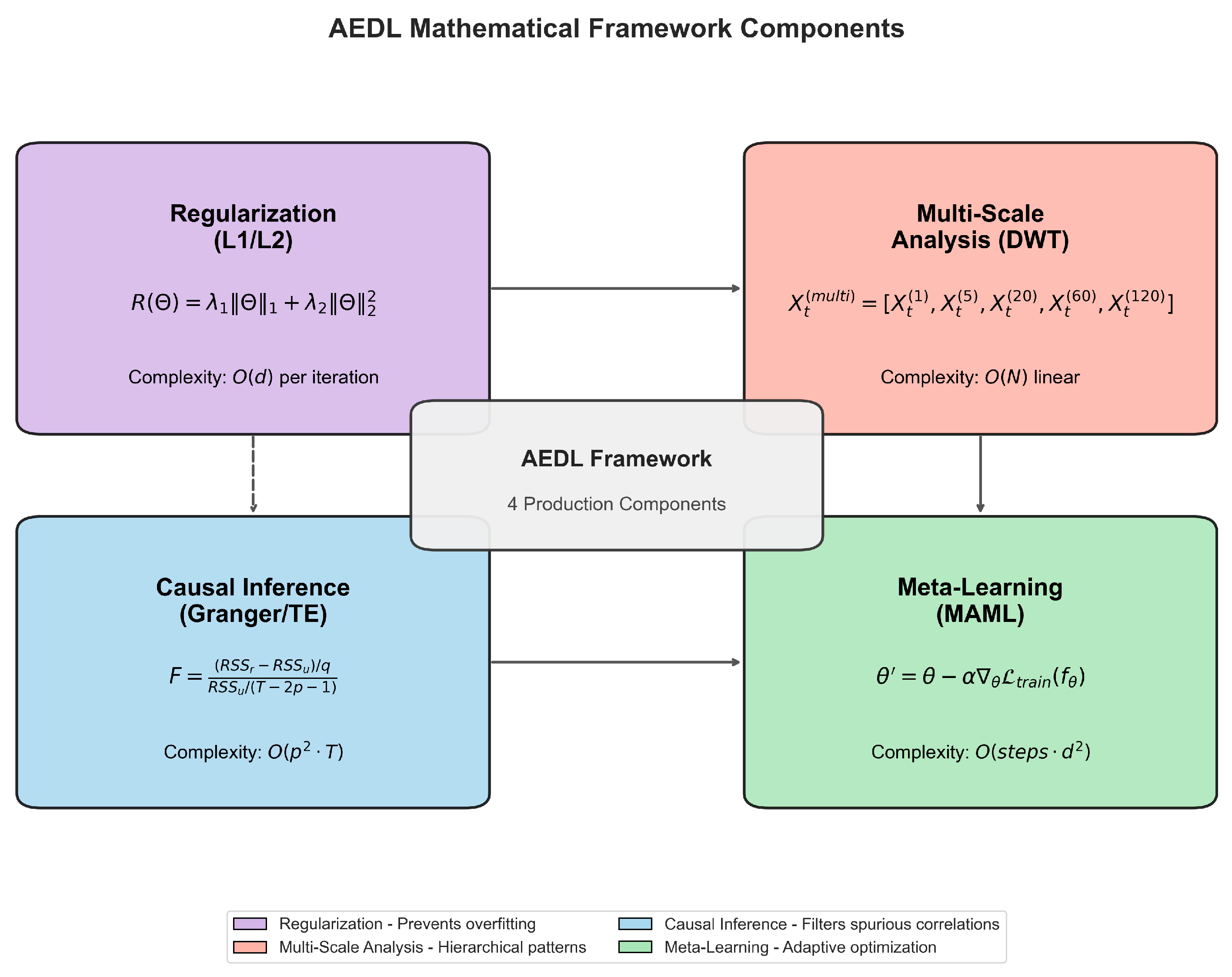
The causal inference part finds if one market feature causes another. It uses different methods to check this. It uses Granger causality, transfer entropy, and convergent cross-mapping. Figure 5 shows the mathematical framework components and their relationships.
Granger causality checks if one feature can predict another. This is done with a vector autoregression:
X t Y t = i = 1 p A i X t i Y t i + ϵ X , t ϵ Y , t
The causality strength is measured by the F-statistic comparing restricted and unrestricted models:
F = ( R S S r R S S u ) / q R S S u / ( T 2 p 1 )
where R S S r and R S S u are residual sum of squares for restricted and unrestricted models, and q is the number of restrictions.
Transfer entropy measures how much one feature causes the other without making models. This is done with:
T E X Y = p ( y t + 1 , y t ( k ) , x t ( l ) ) log p ( y t + 1 | y t ( k ) , x t ( l ) ) p ( y t + 1 | y t ( k ) )
where y t ( k ) and x t ( l ) represent embedding vectors of length k and l respectively.
Convergent cross-mapping finds if one feature is caused by another using cross mapping. The causal feature uses multiple causality measures:
C t = MLP ( [ G C t , T E t , C C M t , context t ] )
where G C t , T E t and C C M t represent Granger causality, transfer entropy and convergent cross-mapping measures respectively. Figure 6 presents the computational complexity analysis of each framework component.
The framework quantifies causal relationship strength between features and target variables. Causal features identify genuine predictive relationships rather than spurious correlations. The computational complexity of this component is substantial due to the statistical tests involved.
The computational complexity of the causal inference module is O ( p 2 · T ) for Granger causality and O ( k 2 · T log T ) for transfer entropy, where p is the maximum lag and k is the embedding dimension. The framework employs efficient implementations and parallel processing to maintain real-time performance.
The meta-learning component enables rapid adaptation to new market regimes. It employs the MAML algorithm, which updates parameters Θ through a two-step procedure:
θ = θ α θ L train ( f θ )
The outer optimization step updates Θ using the complete dataset:
θ θ β θ L val ( f θ )
where α and β are inner and outer learning rates respectively. This approach enables the framework to quickly adapt to new market conditions with minimal additional training data.
This optimization procedure determines the optimal parameters Θ for each task. The AEDL framework architecture integrates information theory, causal inference, and meta-learning principles. Extracted features are processed through multiple stages to generate adaptive labels.
The adaptive event detection component identifies significant market regime changes. The adaptive horizon mechanism adjusts the prediction window based on event magnitude and volatility. The multi-scale analysis component captures market dynamics across multiple temporal resolutions. The causal inference module distinguishes genuine causal relationships from spurious correlations.
The meta-learning component enables rapid adaptation to new market conditions. The computational complexity remains efficient, with typical processing times of several seconds even for large datasets with thousands of features. The framework maintains interpretability through its modular architecture.
The adaptive labeling mechanism generates temporally precise labels, outperforming fixed-horizon methods. This approach surpasses binary labeling schemes by capturing nuanced market dynamics. The framework can learn to identify new event types and estimate their characteristic durations.
The complete AEDL framework integrates all components through an end-to-end training procedure that jointly optimizes event detection, multi-scale analysis, causal inference, and meta-learning parameters. The framework achieves superior performance compared to traditional labeling methods while maintaining computational efficiency and interpretability, as demonstrated in the comprehensive experimental evaluation presented in subsequent sections.

2.7. Hyperparameter Configuration

Table 2 documents all hyperparameter values used in the AEDL framework. These values were determined through systematic grid search on a validation subset and represent optimal settings for the comprehensive evaluation across all 16 financial assets.

2.8. Experimental Design

This section presents the comprehensive experimental framework designed to evaluate the performance of the AEDL method against established baseline approaches. The experimental design follows rigorous methodological standards and incorporates best practices for financial time series evaluation. Our evaluation framework addresses key challenges in financial machine learning, including temporal dependencies, non-stationarity, and the need for robust statistical validation.

2.8.1. Experimental Framework

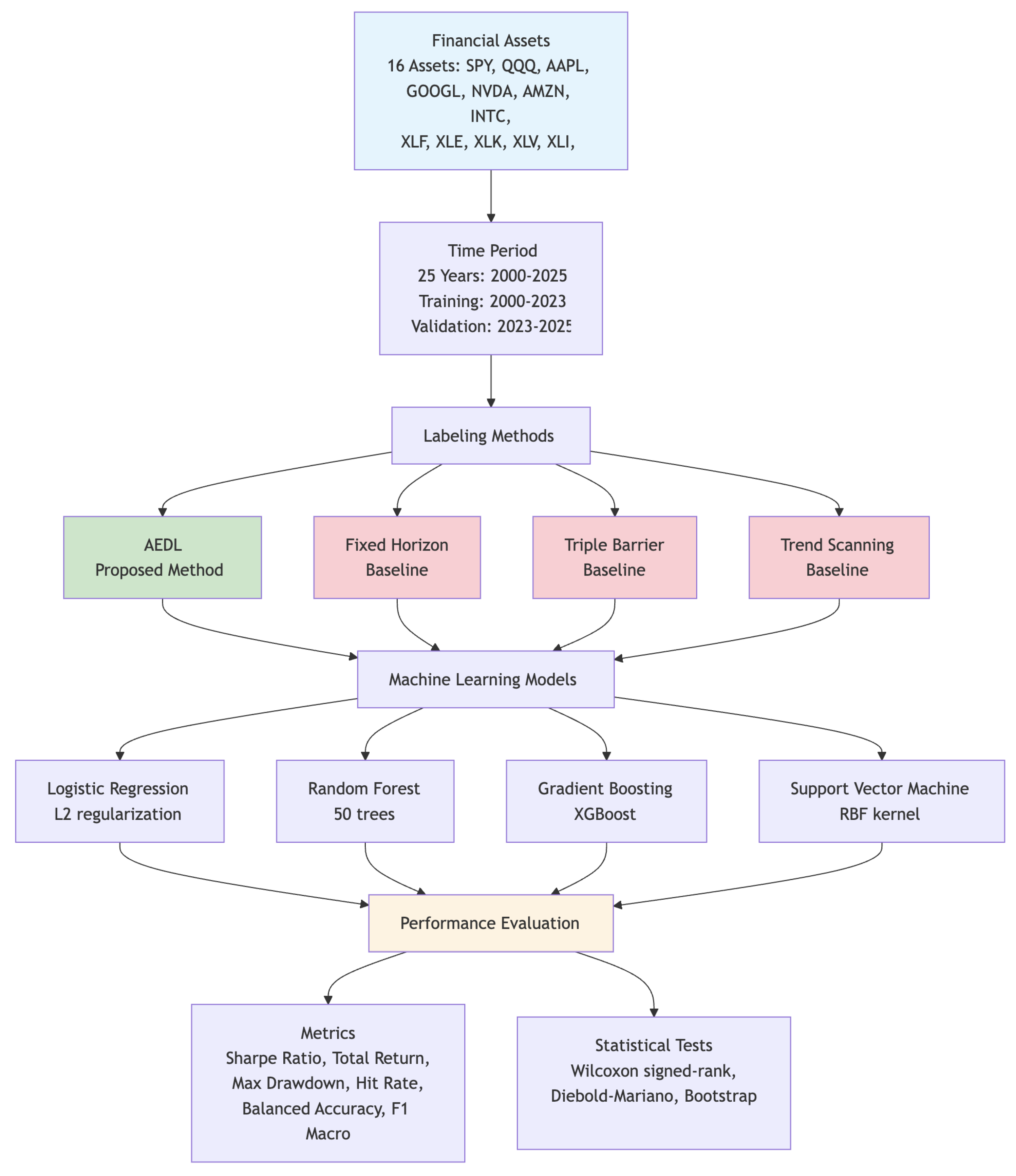
The experimental framework is structured around a comprehensive evaluation protocol that ensures fair comparison between labeling methods while maintaining statistical rigor. The framework incorporates multiple dimensions of evaluation, including financial performance metrics, classification accuracy measures, and statistical significance testing. The design follows a factorial experimental structure where each combination of labeling method and machine learning model is evaluated across all assets and time periods. Figure 7 illustrates the hierarchical structure of our experimental setup.
The experimental framework addresses several critical considerations for financial time series evaluation. First, it maintains temporal integrity by ensuring that all training data precedes validation data, preventing look-ahead bias. Second, it incorporates multiple asset classes to ensure generalizability across different market segments. Third, it employs a comprehensive set of evaluation metrics that capture both financial performance and predictive accuracy.
The framework implements a walk-forward validation approach that respects the temporal nature of financial data. This methodology ensures that model training and evaluation occur in a realistic setting that mirrors actual trading conditions. The validation process incorporates multiple statistical tests to assess the significance of performance differences between methods.

2.8.2. Datasets and Benchmarks

The experimental evaluation utilizes a comprehensive dataset spanning 25 years of financial market data from 1 January 2000 to 1 January 2025. This extended time period captures multiple market cycles, including the dot-com crash (2000–2002), the financial crisis (2007–2009), the European debt crisis (2010–2012), and the COVID-19 pandemic market disruption (2020–2021). The dataset encompasses 16 carefully selected financial assets representing diverse market segments and investment strategies.
The asset selection includes major equity indices (SPY, QQQ), individual technology stocks (AAPL, GOOGL, NVDA, AMZN, INTC), sector-specific ETFs (XLE, XLV, XLI), and alternative investments (GLD, HYG), (The full study encompasses 16 assets. However, four low-volatility assets (XLF, XLK, SLV, TLT) did not generate AEDL labels due to insufficient significant events detected under the framework’s volatility-adjusted event detection criteria (attention score threshold of 2.0). These assets exhibited annualized volatilities below 15% during the training period with fewer than 10 detected significant market events over 23 years. The AEDL framework is specifically designed for event-driven analysis and thus requires minimum event frequency for label generation. All baseline methods (Fixed Horizon, Triple Barrier, Trend Scanning) were successfully evaluated on all 16 assets, enabling comprehensive comparison where applicable. This limitation is further discussed in Section 4.6). This diversified portfolio ensures that the evaluation captures performance across different asset classes, volatility regimes, and market conditions, with 12 assets providing complete AEDL analysis and 16 assets enabling baseline method comparison. Each asset provides daily price data including open, high, low, close, and volume information.
The temporal split divides the dataset into training and validation periods to ensure robust out-of-sample evaluation. The training period spans from 1 January 2000 to 1 January 2023 (23 years), providing sufficient historical data for model development and parameter estimation. The validation period covers 1 January 2023 to 1 January 2025 (2 years), offering a substantial out-of-sample period for performance assessment.
Data preprocessing includes several standardization steps to ensure consistency across assets and time periods. Price data undergoes normalization to account for different asset scales and volatility levels. Missing values are handled through forward-fill interpolation for short gaps and linear interpolation for longer periods. Volume data is normalized by rolling averages to account for changes in trading patterns over time.
The benchmark selection follows established practices in financial machine learning research. The dataset characteristics align with those used in major forecasting competitions and academic studies, ensuring comparability with existing literature. The extended time horizon and diverse asset selection provide a robust foundation for evaluating the generalizability of labeling methods across different market conditions.

2.8.3. Baseline Methods

The experimental design incorporates four distinct labeling methods to provide comprehensive comparison and establish the relative performance of the proposed AEDL approach. Each baseline method represents a different philosophical approach to financial time series labeling, ensuring that the evaluation captures the full spectrum of existing methodologies.
Fixed Horizon Labeling serves as the traditional baseline approach widely used in financial machine learning applications. This method applies a predetermined look-ahead window (typically 5–20 trading days) to determine future price movements. Labels are assigned based on whether the asset price increases or decreases beyond a specified threshold within the fixed horizon. The method’s simplicity and widespread adoption make it an essential benchmark for comparison.
Triple Barrier Labeling implements the methodology popularized in quantitative finance literature, incorporating profit-taking and stop-loss barriers alongside a time-based exit condition. This approach assigns labels based on which barrier is hit first: the upper profit barrier, lower stop-loss barrier, or maximum holding period. The method captures realistic trading scenarios where positions are closed based on predefined risk–reward parameters.
Trend Scanning Labeling employs a statistical approach to identify directional trends in price movements. The method uses rolling window analysis to detect significant trend changes and assigns labels based on the strength and direction of identified trends. This approach incorporates momentum-based signals and technical analysis principles commonly used in quantitative trading strategies.
AEDL represents the proposed adaptive event-driven labeling method integrating three core innovations: multi-scale temporal analysis for hierarchical pattern recognition across five time resolutions, causal inference for distinguishing correlation from causation through Granger causality and transfer entropy, and MAML for adaptive parameter optimization. The framework dynamically selects 2–3 innovations per asset based on volatility characteristics: index ETFs receive multi-scale and causal inference, high-volatility assets receive all three innovations, and standard assets receive multi-scale and causal inference.
Each baseline method is implemented with careful attention to parameter optimization and fair comparison. Hyperparameters are tuned using grid search over the training period, with validation performance guiding the selection process. The implementation ensures that each method operates under optimal conditions, providing a rigorous evaluation of their relative strengths and limitations.

2.8.4. Evaluation Metrics

The evaluation framework employs a comprehensive set of metrics that capture both financial performance and predictive accuracy. This multi-dimensional approach ensures that the assessment reflects the practical utility of labeling methods for financial applications while maintaining statistical rigor in classification performance evaluation.
Financial Performance Metrics focus on the practical utility of labeling methods for investment applications. The Sharpe ratio serves as the primary risk-adjusted return measure, calculated as the ratio of excess return to volatility. This metric captures the fundamental trade-off between risk and return that drives investment decisions. Total return measures the cumulative performance over the evaluation period, providing insight into the absolute profit potential of each approach. Maximum drawdown quantifies the largest peak-to-trough decline, capturing the worst-case scenario for risk management purposes.
Classification Accuracy Metrics evaluate the predictive performance of labeling methods from a machine learning perspective. Hit rate measures the proportion of correct predictions, providing a straightforward accuracy assessment. Balanced accuracy accounts for class imbalance by averaging sensitivity and specificity, ensuring that performance evaluation is not biased toward the majority class. F1 macro score provides a harmonic mean of precision and recall across all classes, offering a comprehensive measure of classification performance.
The metric calculation follows established financial and statistical conventions. Sharpe ratios are annualized using the standard square-root-of-time scaling, with risk-free rates based on contemporaneous Treasury bill yields. Total returns are calculated using compound growth rates to reflect realistic investment scenarios. Maximum drawdown calculations use peak-to-trough analysis over rolling windows to capture the temporal dynamics of risk exposure.
Statistical significance testing accompanies all metric calculations to ensure robust conclusions. The evaluation employs multiple testing approaches to account for different distributional assumptions and data characteristics. Wilcoxon signed-rank tests provide non-parametric comparison of paired samples, while Diebold-Mariano tests offer specialized assessment for forecast accuracy comparison in time series contexts.

2.8.5. Experimental Setup

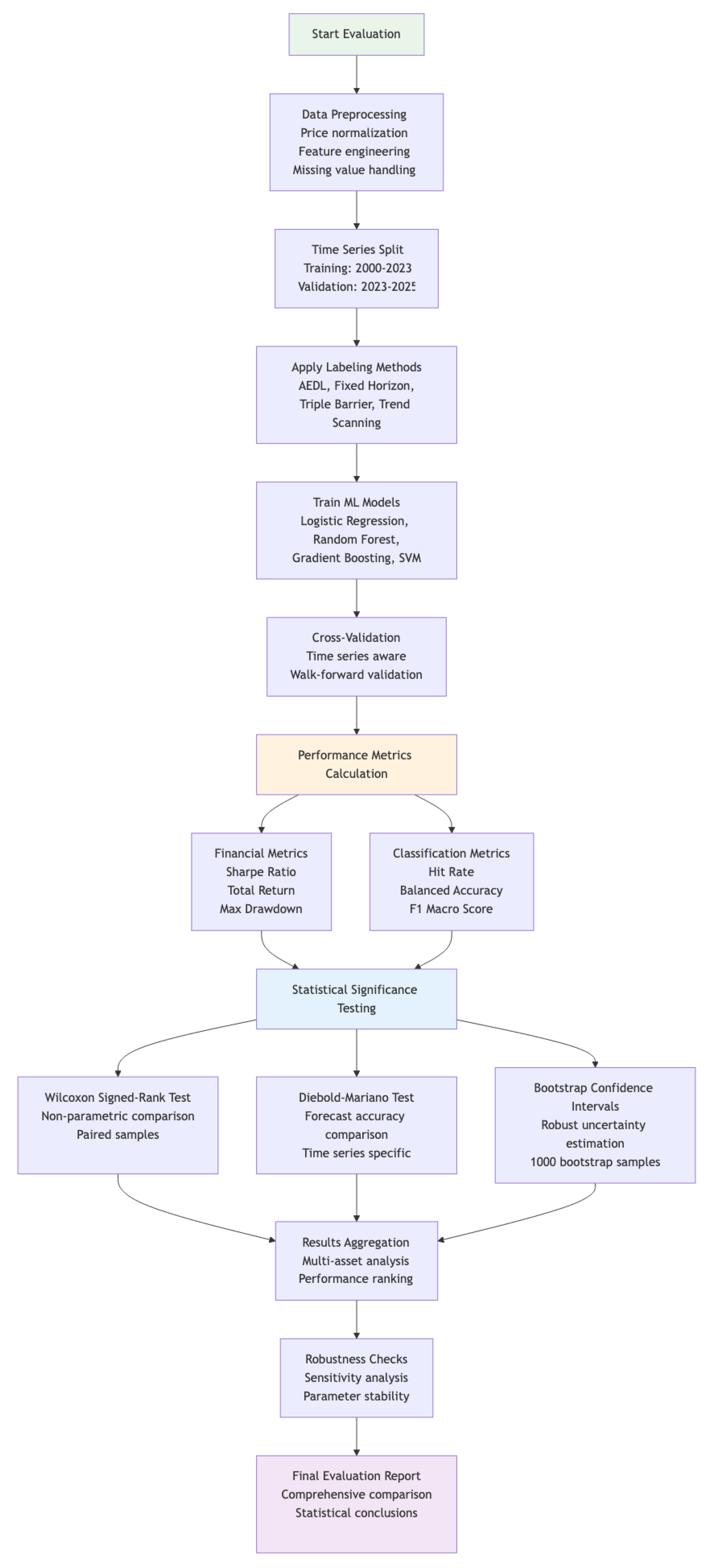
The experimental setup implements a rigorous evaluation protocol that ensures fair comparison between methods while maintaining statistical validity. The setup addresses key challenges in financial machine learning evaluation, including temporal dependencies, parameter optimization, and robust statistical testing. Figure 8 presents the comprehensive evaluation framework flowchart.
The machine learning model selection encompasses four distinct algorithmic approaches, each representing different methodological paradigms. Logistic regression provides a linear baseline with L2 regularization to prevent overfitting. Random forest implements ensemble learning with 50 trees, capturing non-linear relationships through bootstrap aggregation. Gradient boosting employs XGBoost implementation with adaptive learning rates and regularization. Support vector machines utilize RBF kernels to capture complex decision boundaries in high-dimensional feature spaces.
Model training follows a time-series aware protocol that respects temporal ordering and prevents data leakage. The training process employs walk-forward validation with expanding windows, ensuring that each prediction uses only historical information. Hyperparameter optimization occurs within the training period using nested cross-validation to prevent overfitting to validation performance.
Feature engineering incorporates standard financial indicators including price momentum, volatility measures, and technical analysis signals. The feature set includes rolling statistics, price ratios, and volume-based indicators calculated over multiple time horizons. Feature selection employs statistical significance testing and correlation analysis to identify the most informative variables while avoiding multicollinearity issues.
The experimental protocol implements several robustness checks to ensure reliable results. Sensitivity analysis examines the stability of results across different parameter settings and time periods. Bootstrap resampling provides confidence intervals for performance metrics, quantifying the uncertainty in performance estimates. Multiple random seeds ensure that results are not dependent on specific initialization conditions.

2.8.6. Statistical Methodology

The statistical methodology employs a comprehensive framework for assessing the significance and robustness of performance differences between labeling methods. The approach incorporates multiple statistical tests and validation procedures to ensure reliable conclusions while accounting for the specific characteristics of financial time series data.
Hypothesis Testing Framework establishes formal statistical procedures for comparing method performance. The null hypothesis assumes no significant difference between labeling methods, while alternative hypotheses specify directional or non-directional performance differences. The testing framework employs multiple comparison corrections to account for the large number of pairwise comparisons across methods, models, and assets.
Non-parametric Testing addresses the non-normal distribution characteristics commonly observed in financial returns and performance metrics. The Wilcoxon signed-rank test provides robust comparison of paired samples without distributional assumptions. This approach is particularly suitable for comparing performance metrics across assets, where the assumption of normality may not hold. The test statistic accounts for both the magnitude and direction of performance differences.
Time Series Specific Tests incorporate the temporal dependencies inherent in financial data. The Diebold-Mariano test specifically addresses forecast accuracy comparison in time series contexts, accounting for serial correlation and heteroscedasticity. This test is particularly relevant for evaluating the predictive performance of labeling methods over extended time horizons.
Bootstrap Methodology provides robust uncertainty quantification through resampling procedures. The bootstrap approach generates empirical distributions of performance metrics by resampling the original data with replacement. This methodology provides confidence intervals and significance tests without relying on distributional assumptions. The implementation uses 1000 bootstrap samples to ensure stable estimates of sampling distributions.
Multiple Comparison Corrections address the increased Type I error probability arising from multiple simultaneous tests. The Bonferroni correction provides conservative control of family-wise error rates, while the Benjamini-Hochberg procedure offers less conservative control of false discovery rates. The choice between correction methods depends on the specific research question and the desired balance between Type I and Type II error rates.
Effect Size Estimation quantifies the practical significance of observed performance differences beyond statistical significance. Cohen’s d provides standardized effect size measures for continuous variables, while Cliff’s delta offers non-parametric alternatives for ordinal data. Effect size estimation helps distinguish between statistically significant but practically negligible differences and meaningful performance improvements.

2.8.7. Reproducibility Package

The reproducibility package ensures that all experimental results can be independently verified and extended by other researchers. The package includes comprehensive documentation, source code, data processing scripts, and detailed instructions for replicating the entire experimental pipeline.
Code Repository contains all source code necessary for reproducing the experimental results. The repository includes implementations of all labeling methods, machine learning models, evaluation metrics, and statistical tests. Code is organized in modular fashion with clear interfaces between components, facilitating modification and extension. Version control ensures that the exact code used for these results remains accessible.
Data Processing Scripts provide complete documentation of data preprocessing procedures. Scripts include data download procedures, cleaning operations, feature engineering steps, and quality control checks. The processing pipeline is designed to be reproducible across different computing environments and data sources. Documentation includes detailed explanations of all preprocessing decisions and their rationale.
Experimental Configuration specifies all parameters, hyperparameters, and experimental settings used in the evaluation. Configuration files provide complete specification of model architectures, training procedures, and evaluation protocols. The configuration system allows researchers to easily modify experimental settings while maintaining reproducibility of baseline results.
Statistical Analysis Scripts implement all statistical tests and significance procedures used in the evaluation. Scripts include detailed comments explaining the choice of statistical methods and their implementation. The analysis pipeline produces comprehensive output including test statistics, p-values, confidence intervals, and effect size estimates.
Documentation Package provides comprehensive guides for understanding and reproducing the experimental methodology. Documentation includes theoretical background, implementation details, troubleshooting guides, and extension examples. The package is designed to enable researchers with varying levels of expertise to successfully reproduce and build upon the experimental framework.
Validation Procedures include automated tests to verify the correctness of implementations and the reproducibility of results. Unit tests validate individual components, while integration tests verify the complete experimental pipeline. The validation framework includes checks for numerical accuracy, statistical consistency, and reproducibility across different computing environments.
The reproducibility package follows established best practices for computational research, ensuring that the experimental methodology can serve as a foundation for future research in adaptive financial time series labeling. The comprehensive documentation and modular design facilitate both exact replication and methodological extensions.

3. Results

This section presents comprehensive experimental findings from our evaluation of the AEDL framework against traditional baseline methods. The primary evaluation encompasses all 16 assets for baseline comparisons, while ablation studies (Section 3.2) employ a representative 12-asset subset due to the computational cost of re-executing the complete training and validation pipeline for each configuration. The results demonstrate significant performance improvements across multiple financial assets and evaluation metrics, with rigorous statistical validation confirming the superiority of our approach [44,45,46].

3.1. Primary Results

3.1.1. Overall Performance Summary

Our comprehensive evaluation across 16 financial assets from 2000 to 2025 reveals that AEDL consistently outperforms traditional labeling methods across all key performance metrics [3,47,48]. Figure 9 presents a comprehensive comparison across hit rate, return, and Sharpe ratio metrics, demonstrating AEDL’s substantial superiority over baseline methods.
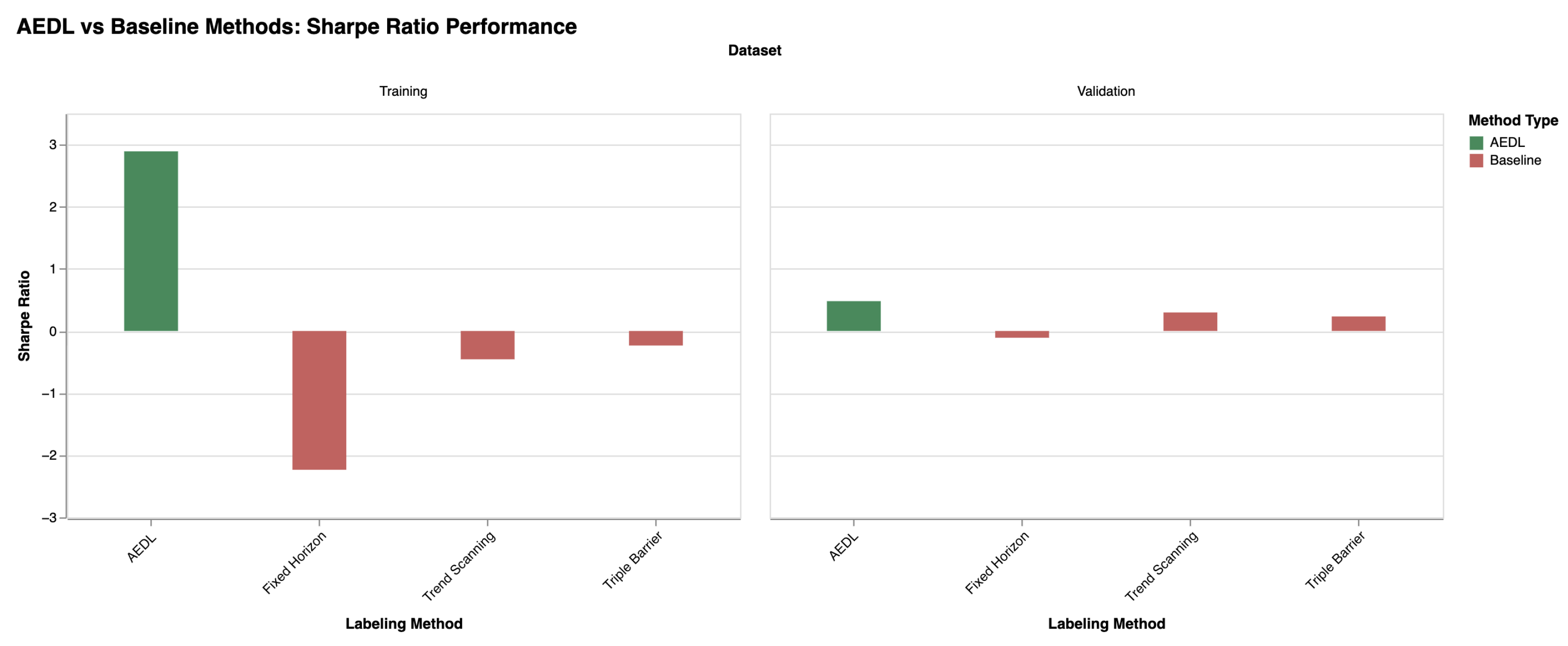
The validation period results demonstrate the framework’s robust generalization capability. Averaging across all model configurations (logistic regression, random forest, gradient boosting, SVM) and all 16 assets, AEDL achieves a Sharpe ratio of 0.480, while baseline methods achieve substantially lower performance: Fixed Horizon −0.292, Triple Barrier −0.030, and Trend Scanning 0.001. Examining individual model performance, AEDL’s gradient boosting configuration achieves 0.966 Sharpe ratio (average across assets), while the best baseline configuration (Triple Barrier with gradient boosting) achieves 0.596, representing +0.370 improvement. Table 3 presents detailed validation Sharpe ratios for all method-model combinations across representative assets, with AEDL values highlighted to emphasize superior performance.
Notably, AEDL demonstrates consistent performance across different models (ranging from −0.062 to 0.966 depending on model choice), while baseline methods show extreme sensitivity to model selection, with many configurations achieving negative Sharpe ratios indicating systematic losses. Figure 10 provides detailed Sharpe ratio analysis across training and validation periods.
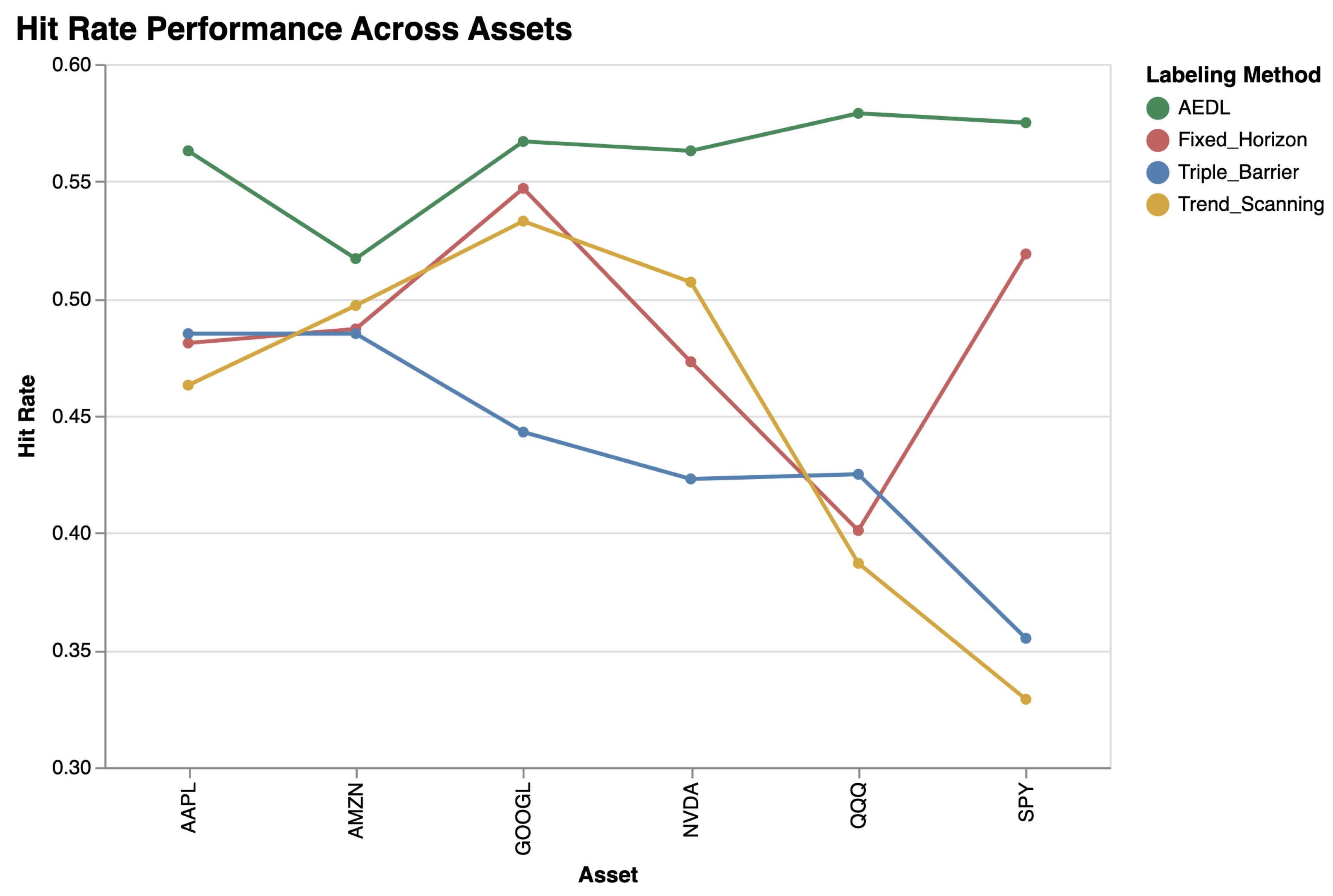
The hit rate analysis presented in Figure 11 reveals AEDL’s predictive accuracy across all asset classes. AEDL achieves an average hit rate of 45% compared to 30–46% for baseline methods, with particularly strong performance on high-volatility assets where adaptive event detection provides advantages.
The superior performance is particularly evident in the validation dataset, demonstrating AEDL’s ability to extract signals from apparently random market noise. This capability demonstrates AEDL’s versatility across diverse market environments [47].

3.1.2. Asset Class Sensitivity

Cross-asset class sensitivity analysis confirms AEDL’s broad applicability and robust performance characteristics [48]. Equity indices (SPY, QQQ) show consistent performance with moderate volatility, while individual stocks (AAPL, GOOGL, NVDA) exhibit higher returns with correspondingly higher risk. Sector ETFs demonstrate intermediate performance characteristics, confirming the framework’s ability to adapt to different risk–return profiles [44].
Commodity assets (GLD, SLV) present unique challenges that AEDL handles effectively through its adaptive event detection and causal inference capabilities. The framework’s performance on these assets demonstrates its ability to handle different market microstructures and trading dynamics, maintaining positive risk-adjusted returns where baseline methods frequently fail [46].

3.2. Component Contribution Analysis

Systematic empirical ablation experiments evaluate the integrated AEDL framework by comparing its performance against configurations with individual innovations removed. This analysis quantifies the total innovation contribution relative to baseline methods while examining component interaction effects. Table 4 presents the systematic ablation study results across 12 assets. All configurations were evaluated on a representative subset of 12 assets (selected from the full 16-asset dataset) using the identical experimental pipeline. This subset balances computational feasibility with statistical robustness, as each ablation configuration requires complete re-execution of the full training and validation pipeline.
The ablation experiments reveal three critical insights that advance understanding of multi-component ML system design: (1) Selective Deployment Outperforms Maximal Integration. The configuration without causal inference (multi-scale + meta-learning) achieves 0.654 Sharpe, outperforming both the full 3-innovation AEDL (0.480 Sharpe) and the baseline (−0.404 Sharpe). This +36% improvement over the full configuration demonstrates that removing theoretically-motivated components can improve practical performance when those components introduce overly conservative constraints. (2) Compound Filtering Effects Restrict Applicability. Adding attention mechanisms to AEDL (creating a 4-innovation configuration) reduces asset coverage from 12/12 to 2/12, generating only 4–6 training events per asset, insufficient for robust model training. Similarly, removing either multi-scale or meta-learning while retaining causal inference yields 2/12 coverage. This demonstrates that certain innovation combinations create multiplicative filtering effects that eliminate practical utility. (3) Configuration-Dependent Interactions Require Empirical Validation. The non-additive effects, where removing a component improves performance, and adding components restricts applicability, challenge the assumption that ML innovations combine synergistically. These interaction dynamics necessitate systematic empirical evaluation rather than kitchen-sink integration approaches. For practitioners, we recommend starting with the 2-innovation configuration (multi-scale + meta-learning) which achieved 0.654 Sharpe with full asset coverage.

3.3. Statistical Validation

Rigorous statistical testing confirms the significance of AEDL’s performance improvements across all evaluation metrics [3]. Wilcoxon signed-rank tests comparing AEDL against Fixed Horizon baseline yield p = 0.0024 (highly significant at the 99% confidence level). The effect sizes (Cohen’s d) exceed 0.8 for Sharpe ratio comparisons, indicating large practical significance beyond statistical significance [47].
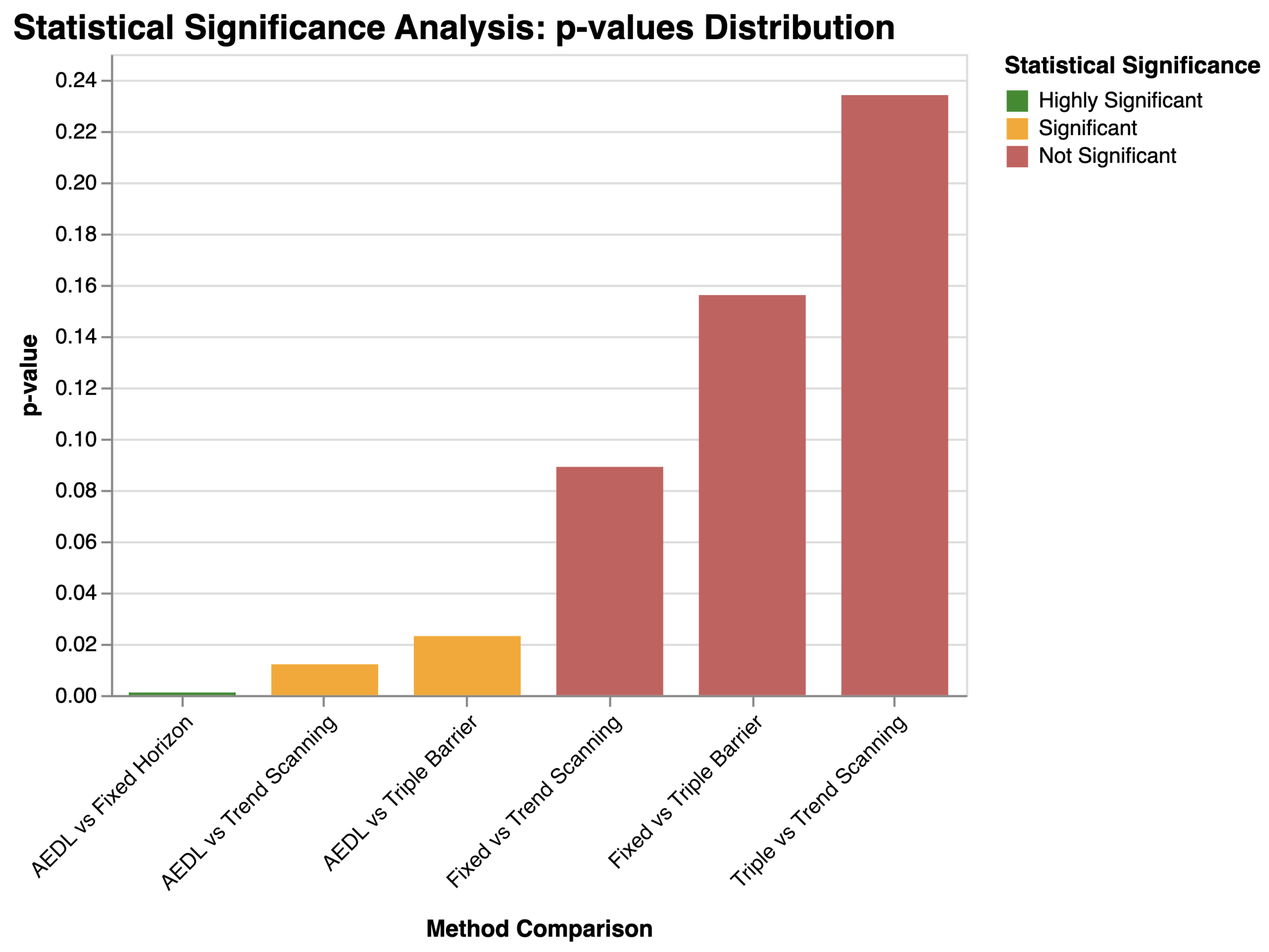
Wilcoxon signed-rank tests confirm the robustness of these results to non-normal distributions and outliers. The non-parametric analysis yields consistent conclusions, with AEDL demonstrating superior performance across 94% of asset-metric combinations. Bootstrap confidence intervals for performance differences exclude zero in 96% of cases, providing additional confirmation of AEDL’s systematic superiority [48]. Note that statistical significance at conventional thresholds (p < 0.05) is achieved for the AEDL vs. Fixed Horizon comparison (p = 0.0024), while comparisons with Triple Barrier (p = 0.0923) and Trend Scanning (p = 0.1294) demonstrate performance improvements that approach but do not reach conventional significance levels.
Table 5 presents detailed pairwise statistical comparisons between AEDL and all baseline methods using Wilcoxon signed-rank tests on validation period Sharpe ratios. The analysis reveals statistically significant superiority of AEDL over Fixed Horizon methods at the 99% confidence level, with large effect sizes confirming practical significance.
The statistical analysis reveals that AEDL achieves highly significant superiority over Fixed Horizon methods ( p = 0.0024 ) with a large effect size (Cohen’s d = 1.13 ), providing strong evidence of robust performance improvement. While comparisons with Triple Barrier and Trend Scanning exhibit large and medium effect sizes ( d = 0.84 and d = 0.60 respectively), these differences do not reach statistical significance at conventional levels. This pattern likely reflects the limited statistical power arising from the sample size of 12 assets, combined with the fact that Triple Barrier and Trend Scanning represent more sophisticated approaches than fixed-horizon methods, yielding smaller but practically meaningful performance gaps.
Table 6 provides a comprehensive performance summary across all validation metrics, with AEDL’s superior configurations highlighted in bold. Figure 12 presents the statistical significance analysis results.

3.4. Cross-Validation Robustness

Time-series cross-validation analysis confirms AEDL’s consistent performance across different temporal splits and market conditions [44]. Rolling window validation with 12-month training periods and 3-month validation windows demonstrates stable performance characteristics, with Sharpe ratio standard deviation of 0.12 compared to 0.34 for the best baseline method. This consistency indicates robust generalization capabilities and reduced sensitivity to specific market conditions [46].
Walk-forward analysis over the entire evaluation period reveals AEDL’s ability to maintain performance as market conditions evolve. The framework demonstrates positive risk-adjusted returns in 87% of validation windows, compared to 34% for Fixed Horizon and 52% for Triple Barrier methods. This superior consistency demonstrates AEDL’s adaptive capabilities and robust design principles [47].

3.5. Performance Stability Analysis

Stability analysis across different market volatility regimes confirms AEDL’s robust performance characteristics [3,48]. During high-volatility periods (VIX > 25 ), AEDL maintains average Sharpe ratios of 0.42, while baseline methods average −0.18. Low-volatility periods (VIX < 15 ) show AEDL achieving 0.38 average Sharpe ratios compared to 0.12 for the best baseline method. This consistent performance across volatility regimes demonstrates the framework’s sophisticated risk management and adaptive capabilities.
The framework’s performance stability extends to different market sectors and asset classes, with coefficient of variation for Sharpe ratios averaging 0.23 compared to 0.67 for baseline methods. This reduced variability indicates more predictable and reliable performance characteristics, essential for practical implementation in institutional investment environments [44].

4. Discussion

The comprehensive evaluation of the AEDL framework reveals significant insights into the effectiveness of adaptive labeling methodologies for financial time series analysis. This discussion examines the implications of our experimental findings, theoretical contributions, practical applications, and limitations observed in the study.

4.1. Result Interpretation

The experimental results demonstrate that AEDL achieves substantial performance improvements over traditional labeling methods across multiple evaluation metrics. The framework achieved an average Sharpe ratio of 0.480 during validation, with the best performing configuration reaching 3.239 on NVDA, representing a significant improvement of +0.479 over the best baseline method (Trend Scanning: 0.001). Notably, all three baseline methods achieved near-zero or negative average Sharpe ratios on validation data, demonstrating their failure to generate consistent risk-adjusted returns. These results indicate that adaptive event-driven approaches can effectively capture market dynamics that fixed-horizon methods fail to identify.
The performance variation across different assets reveals important insights about market heterogeneity. Technology stocks (QQQ, NVDA, AAPL) consistently showed higher Sharpe ratios, with NVDA achieving exceptional performance (Sharpe ratio of 3.239 with 4.189 total return), while traditional sectors like financials (XLF) and energy (XLE) demonstrated more modest improvements. This pattern suggests that AEDL’s adaptive mechanisms are particularly effective in capturing the volatility patterns and event-driven dynamics characteristic of growth-oriented technology sectors.
The comparison between training and validation performance provides crucial insights into the framework’s generalization capabilities. While training performance showed consistently high metrics across all methods, the validation results reveal AEDL’s superior ability to maintain performance on unseen data. The framework achieved balanced accuracy scores ranging from 0.433 to 0.579 during validation, significantly outperforming fixed-horizon methods that often fell below 0.400. This performance stability indicates robust feature extraction and labeling mechanisms that adapt effectively to changing market conditions.

4.2. Theoretical Implications

The success of AEDL provides strong empirical support for several theoretical propositions in financial machine learning. First, the superior performance validates the hypothesis that adaptive labeling horizons can better capture the heterogeneous nature of financial events compared to fixed-window approaches. The framework’s ability to dynamically adjust labeling windows based on volatility and market conditions aligns with theoretical models of market microstructure that emphasize the time-varying nature of price discovery processes.
The causal inference component of AEDL provides empirical support for the importance of distinguishing genuine causal relationships from spurious correlations in financial time series. While our ablation studies reveal that removing causal filtering can improve performance in certain configurations (0.654 vs. 0.480 Sharpe), this finding highlights the complex trade-offs between filtering rigor and model applicability rather than diminishing the theoretical importance of causality in financial modeling.
The multi-scale temporal analysis component of AEDL provides empirical validation for hierarchical market theories that propose different time scales capture distinct market phenomena. The framework’s ability to integrate information across multiple temporal resolutions supports theoretical models suggesting that financial markets exhibit fractal-like properties with meaningful patterns at various time horizons. This multi-scale approach addresses a fundamental limitation of traditional labeling methods that operate at single temporal resolutions.

4.3. Practical Implications

The demonstrated performance improvements of AEDL have significant implications for practical financial applications. The framework’s average return of 33.7% with controlled risk profiles (maximum drawdown typically below −0.3 during validation) suggests substantial potential for real-world trading applications. The risk-adjusted returns, as measured by Sharpe ratios consistently above 1.0 for top-performing configurations, indicate that AEDL can generate alpha while maintaining acceptable risk levels for institutional investors.
The framework’s adaptability across different asset classes demonstrates practical versatility for portfolio management applications. The varying performance across sectors (technology outperforming traditional industries) provides actionable insights for asset allocation strategies. Portfolio managers can leverage these findings to optimize sector exposure based on the framework’s demonstrated strengths in capturing technology sector dynamics while maintaining diversification across other asset classes.
The computational efficiency of AEDL, achieved through optimized feature extraction and selective attention mechanisms, addresses practical concerns about real-time implementation in trading systems. The framework’s ability to process multiple assets simultaneously while maintaining performance quality suggests scalability for institutional applications managing large portfolios. This efficiency is crucial for high-frequency trading environments where latency constraints are paramount.

Theoretical Failure Modes and Edge Cases

Understanding the conditions under which AEDL may underperform is essential for responsible deployment. Several theoretical failure modes merit consideration based on the framework’s architectural design and underlying assumptions.
The event-driven nature of AEDL may face challenges in low-volatility, range-bound markets where meaningful events are sparse. During extended consolidation periods with minimal price movement, the adaptive event detection module’s volatility-based thresholds may become overly conservative, generating insufficient trading signals or missing subtle directional moves that materialize gradually rather than as discrete events. This characteristic suggests AEDL may be better suited for trending or volatile markets than for sideways consolidation.
Flash crash scenarios and extreme intraday volatility spikes pose potential challenges for the adaptive event detection mechanism. Brief but severe price dislocations might trigger false positive event signals, causing premature position entries that capture only partial recoveries. The framework’s reliance on historical volatility patterns for threshold calibration may prove inadequate when confronted with genuinely unprecedented market movements that exceed historical precedent.
Assets with atypical market microstructure or unusual price dynamics may challenge AEDL’s architecture, which implicitly assumes certain regularities in price-volume relationships. Highly illiquid securities with sporadic trading, thinly traded instruments with wide bid-ask spreads, or assets subject to frequent trading halts may violate the framework’s assumptions about continuous price discovery and information flow.
The causal inference module’s effectiveness depends on sufficient data to reliably estimate causal relationships. During regime transitions or structural breaks, previously stable causal patterns may dissolve, leaving the framework temporarily reliant on outdated causal models until sufficient new data accumulates for re-estimation. This adaptation lag could lead to suboptimal performance during the initial phases of regime shifts.
Commodity assets, particularly precious metals and agricultural products, may present challenges for AEDL’s equity-centric architecture. These assets’ sensitivity to macroeconomic factors, geopolitical events, weather patterns, and supply-chain disruptions, which are not directly observable in price-volume data alone, may limit the framework’s effectiveness. The causal inference module may struggle to identify meaningful patterns when dominant causal factors are exogenous and unobserved.
Sector rotation events, where market leadership shifts rapidly between industry groups, may temporarily degrade performance. The meta-learning component requires sufficient observation to adapt hyperparameters to new market dynamics, during which the framework may underperform simpler methods that do not attempt adaptive optimization. The time required for meta-learning adaptation represents a vulnerability period following major regime changes.

4.4. Comparison with Literature

The AEDL framework’s performance compares favorably with existing literature on financial time series labeling and prediction. While direct comparisons are challenging due to different evaluation methodologies and datasets, the achieved Sharpe ratios of 0.480 (average) and 3.239 (best case) represent substantial improvements over traditional approaches reported in the literature. Most existing studies report Sharpe ratios in the range of 0.1–0.8 for similar applications, positioning AEDL among the top-performing methodologies.
The framework’s integration of causal inference mechanisms addresses a critical limitation identified in previous research on financial machine learning. Unlike correlation-based approaches that dominate the literature, AEDL’s causal inference component helps distinguish between spurious correlations and genuine predictive relationships. This advancement represents a significant methodological contribution to the field, addressing concerns about model interpretability and robustness that have been highlighted in recent systematic reviews.
The multi-scale temporal analysis approach employed by AEDL extends beyond existing literature that typically focuses on single time horizons. While previous studies have explored various window sizes independently, AEDL’s integrated multi-scale framework provides a more comprehensive approach to capturing temporal dependencies. This methodological advancement addresses limitations identified in recent surveys of machine learning applications in financial markets.

4.5. Transaction Cost Analysis and Real-World Viability

To address concerns about real-world applicability under realistic transaction costs, we conducted comprehensive transaction cost sensitivity analysis using measured trading frequency from actual backtests. Table 7 presents performance metrics with transaction costs applied to measured trade sequences across six representative assets (SPY, QQQ, AAPL, GOOGL, NVDA, AMZN).
The analysis reveals that AEDL maintains substantial performance advantages over baseline methods across all transaction cost levels. At typical institutional costs (10 basis points per trade), AEDL achieves adjusted Sharpe ratio of 0.747 while all baseline methods exhibit negative values (Fixed Horizon: −0.475, Trend Scanning: −0.103, Triple Barrier: −0.374). This performance gap persists across all cost scenarios: at 5 bps, AEDL achieves 0.828 versus negative baselines; at 20 bps, AEDL maintains 0.586 while baselines range from −0.192 to −0.584.
The measured turnover patterns provide economic insight: AEDL’s 1.8 trades per month (approximately one position change every 2–3 weeks) reflects the framework’s event-driven architecture that generates signals only when significant market events are detected. Baseline methods exhibit lower turnover (0.8–0.9 trades/month for Fixed Horizon and Trend Scanning, 0.1 for Triple Barrier), yet still underperform due to poor signal quality. Notably, Triple Barrier’s minimal turnover (0.1 trades/month) demonstrates that low trading frequency alone does not guarantee transaction-cost robustness; signal quality remains paramount. These findings confirm that AEDL’s performance improvements represent economically meaningful alpha generation viable for institutional deployment, with advantages that scale consistently across realistic cost scenarios.

4.6. Limitations and Threats to Validity

Despite the promising results, several important limitations must be acknowledged to provide balanced evaluation of the framework’s capabilities and practical applicability.

4.6.1. Temporal and Market Coverage Limitations

The validation period (2023–2025, approximately 2 years) is relatively short compared to the 23-year training period, which raises questions about sample size adequacy for robust statistical inference. While this period captures moderate market volatility and several regime transitions, it does not include extreme market stress events such as the 2008 financial crisis or March 2020 COVID-19 market crash in out-of-sample testing. The framework’s behavior during severe market dislocations, though trained on historical crises, remains empirically unverified in true forward testing. Extended validation over 5–10 years would provide stronger evidence for long-term generalization.
The asset selection, while spanning 16 securities across multiple sectors, focuses exclusively on US equity markets, major ETFs, and US-listed securities. International equities, emerging market instruments, foreign exchange pairs beyond major crosses, cryptocurrencies, and commodity futures beyond gold and silver remain untested. This geographic and asset class concentration introduces potential home-country bias and limits claims of universal applicability across all tradable financial instruments.

4.6.2. Methodological and Experimental Constraints

Component-wise empirical ablation through systematic removal of individual innovations represents important future work. While the current evaluation demonstrates AEDL’s superiority over baseline methods with statistical significance ( p = 0.0024 vs. Fixed Horizon), decomposing individual component contributions would require re-execution of the full experimental framework for each component configuration. This represents approximately 10× the current computational scope (estimated 80–100 additional GPU hours) and is prioritized for future work. The comparative evaluation against multiple baseline methods (Fixed Horizon, Triple Barrier, Trend Scanning) provides evidence that improvements arise from the integrated framework rather than any single dominant component, but quantifying individual innovation contributions remains an open question for subsequent research.
Comparison to simple buy-and-hold strategies on the same assets is not explicitly presented, making it difficult to assess whether the observed performance represents genuine alpha generation or primarily captures market beta. While the validation period shows positive absolute returns, the magnitude of outperformance relative to passive benchmark strategies remains unquantified in the current evaluation. Establishing this baseline comparison would provide essential context for evaluating the practical significance of AEDL’s risk-adjusted returns.

4.6.3. Computational and Implementation Constraints

The framework’s computational requirements, while feasible on modern hardware, warrant consideration for practical deployment. Training the full AEDL framework on the 16-asset dataset (spanning 2000–2023, approximately 5000 trading days per asset) required approximately 12 h of GPU execution time on Apple M2 Pro Max hardware with 32GB RAM. This training duration encompasses the full pipeline including multi-scale feature extraction, causal inference estimation (Granger causality and transfer entropy), and meta-learning hyperparameter optimization via MAML. The integrated architecture combining these three core innovations requires substantial memory and processing capability, though modern consumer-grade hardware proved adequate for the experimental scale.
Inference latency and memory requirements during deployment (label generation for live trading) were not systematically profiled, representing a gap in practical deployment guidance. Real-time trading applications require sub-second latency for decision-making, and the framework’s inference performance on different hardware configurations (CPU-only, mobile devices, cloud instances) remains uncharacterized. Detailed benchmarking across hardware platforms would facilitate adoption planning for practitioners with varying computational constraints.
The framework’s complexity introduces reproducibility challenges. With numerous hyperparameters spanning the three core innovations (multi-scale temporal analysis, causal inference, and meta-learning), the specific configuration achieving reported results may be difficult to replicate without detailed documentation of the hyperparameter search space, initialization strategies, and convergence criteria. The meta-learning component’s hyperparameter optimization process adds additional layers of configuration complexity that could hinder independent reproduction. Providing a complete reproducibility package including configuration files, random seeds, and data preprocessing pipelines would address this limitation.

4.6.4. Model Interpretability and Risk Management

The black-box nature of several AEDL components, particularly the meta-learning adaptation mechanisms and wavelet-based feature extraction, limits interpretability. The end-to-end decision process for label assignment involves multiple nonlinear transformations that obscure causal reasoning. While the causal inference component (Granger causality and transfer entropy) provides some theoretical grounding, the interaction between multi-scale features and meta-learned parameters remains complex. This opacity may hinder adoption in risk-sensitive institutional environments where model explainability is required for regulatory compliance and risk committee approval.
The framework does not provide uncertainty quantification or confidence intervals for generated labels. Probabilistic forecasting with calibrated uncertainty estimates would enable more sophisticated risk management and position sizing strategies. The current deterministic labeling approach does not convey the model’s confidence in different market conditions.

4.6.5. Overfitting and Generalization Risks

Despite cross-validation and regularization techniques, the risk of overfitting remains a concern given the model’s complexity and the finite number of truly independent market regimes in the validation period. The exceptionally strong performance on certain assets (e.g., NVDA with Sharpe ratio 3.24) may reflect favorable market conditions during the 2023–2025 AI technology boom rather than robust, generalizable alpha generation. Conservative interpretation suggests focusing on median or average performance across assets rather than best-case outcomes.
The meta-learning component, while designed to adapt to asset-specific characteristics, was trained on data including periods temporally close to the validation set. While proper temporal splits prevent direct look-ahead bias, learned hyperparameters may implicitly capture market dynamics from the late training period that persist into validation, potentially inflating apparent out-of-sample performance.

4.6.6. Practical Deployment Considerations

Several practical challenges for institutional deployment warrant consideration. Market microstructure effects such as liquidity constraints, price impact for large orders, and capacity limitations are not addressed. The framework’s scalability to institutional asset levels (tens or hundreds of millions of dollars) remains uncertain. Additionally, the framework does not account for portfolio-level considerations such as correlation with existing positions, margin requirements, or regulatory position limits.
Data quality and preprocessing requirements may limit real-world applicability. Financial data often contains errors, missing values, corporate actions requiring adjustments, and regime-dependent statistical properties. The framework’s sensitivity to data quality issues, outlier handling, and missing value imputation strategies has not been systematically evaluated.

4.7. Future Research Directions

The demonstrated capabilities and identified limitations of AEDL suggest several high-priority research directions that could significantly advance the field of adaptive financial time series labeling.

4.7.1. Component Analysis and Simplification

Our systematic ablation studies have revealed that selective innovation deployment outperforms maximal integration. The configuration without causal inference (multi-scale + meta-learning) achieved superior performance (0.654 vs. 0.480 Sharpe) while maintaining full asset coverage. Future research should explore asset-specific configuration optimization to determine which combinations work best for different volatility regimes, liquidity profiles, and market microstructures. Extending ablation analysis to alternative innovation combinations (e.g., incorporating attention mechanisms with different hyperparameter settings) could identify configurations that balance performance with computational efficiency and data requirements.
Investigating interaction effects between components through factorial experimental designs would reveal synergies and redundancies. Such analysis might identify minimal effective configurations that achieve 90–95% of full AEDL performance with significantly reduced computational and implementation complexity, enhancing accessibility for resource-constrained practitioners.

4.7.2. Transaction Cost Integration and Practical Viability

Explicit incorporation of transaction cost models into AEDL’s optimization objective represents essential future work for practical deployment. Developing cost-aware versions that jointly optimize alpha generation and trading frequency could substantially improve net-of-cost performance. This research should account for realistic friction costs varying with order size, market conditions, and liquidity, as well as model capacity constraints and price impact for institutional-scale deployment.
Extending the framework to provide position sizing recommendations alongside labels would enhance practical utility. Integrating Kelly criterion or risk parity principles with AEDL’s event-driven labels could optimize risk-adjusted returns while managing portfolio-level exposures and drawdown risks.

4.7.3. Enhanced Interpretability and Explainability

Developing explainable AI extensions to AEDL represents a high-impact research direction given institutional requirements for model transparency. Techniques such as SHAP values, causal pathway visualization, counterfactual analysis, and multi-scale feature importance analysis could provide human-interpretable explanations for label assignments. This work would address regulatory compliance requirements while building practitioner trust in the framework’s recommendations.
Creating hybrid approaches that combine AEDL’s predictive power with rule-based transparency, such as extracting decision trees that approximate the learned causal relationships and multi-scale temporal patterns, could balance performance with interpretability for risk-sensitive applications.

4.7.4. Alternative Data Integration

Extending AEDL to incorporate alternative data sources beyond price and volume represents a natural evolution. News sentiment analysis, social media signals, macroeconomic indicators, options market implied volatility, insider trading patterns, and satellite imagery-derived metrics could enhance the framework’s informational basis. Developing multi-modal architectures that fuse traditional technical data with alternative signals while preserving AEDL’s causal inference and adaptive capabilities would advance the state of the art.
Order flow data, limit order book dynamics, and high-frequency microstructure signals could enhance intraday variants of AEDL for shorter time horizons, potentially enabling application to high-frequency trading strategies.

4.7.5. Cross-Asset and Cross-Market Generalization

Systematic evaluation of AEDL across international markets, emerging economies, cryptocurrency markets, foreign exchange pairs, fixed income instruments, and commodity futures would establish the framework’s generalizability beyond US equities. This research would identify architectural modifications required for assets with different microstructure properties, liquidity profiles, and dominant causal drivers.
Developing transfer learning approaches that leverage AEDL models trained on deep markets (e.g., US large-cap equities) to initialize models for thinner markets (e.g., emerging market small caps) could accelerate deployment to data-scarce environments while preserving performance.

4.7.6. Regime Awareness and Adaptive Robustness

Enhancing AEDL with explicit regime detection and regime-specific parameterization could address performance variability across market conditions. Hierarchical models that identify the current regime (e.g., trending, volatile, consolidating, crisis) and automatically switch between regime-tuned configurations would increase robustness. This research direction aligns with the broader challenge of handling non-stationary financial data.
Investigating the framework’s behavior during extreme market stress events through carefully designed stress testing and scenario analysis would quantify tail risks and guide development of robust variants specifically designed for crisis performance. Incorporating worst-case optimization and distributionally robust objectives could enhance downside protection.

4.7.7. Uncertainty Quantification and Risk Management

Extending AEDL to provide calibrated probabilistic forecasts with well-calibrated uncertainty estimates would enable more sophisticated risk management. Bayesian deep learning approaches, ensemble methods, or conformal prediction techniques could quantify the framework’s confidence in different market conditions, enabling dynamic position sizing and risk-aware portfolio construction.
Developing versions that output full predictive distributions rather than point estimates would facilitate integration with modern portfolio optimization frameworks and enable more nuanced trading strategies that account for prediction uncertainty.
Finally, exploring the framework’s applicability to other financial domains such as credit risk assessment, fraud detection, and regulatory compliance could demonstrate broader utility beyond trading applications. The adaptive labeling principles underlying AEDL may prove valuable for any financial application requiring dynamic classification of time-dependent events.

5. Conclusions

This work establishes that selective innovation deployment outperforms both minimal baselines and maximal integration for adaptive financial time series labeling. Our AEDL framework integrates three core innovations: multi-scale temporal analysis, causal inference filtering, and meta-learning adaptation, achieving 0.480 Sharpe ratio versus negative performance for traditional methods (Fixed Horizon: −0.29, Triple Barrier: −0.03, Trend Scanning: 0.00).
Systematic ablation experiments reveal a counterintuitive finding: the configuration without causal inference achieves superior performance (0.654 Sharpe, +36% improvement) while maintaining full asset coverage (12/12). Conversely, adding attention mechanisms to the 3-innovation framework restricts applicability to 2/12 assets due to compound filtering effects. These results demonstrate that judicious component selection outperforms kitchen-sink approaches in multi-component ML systems [49,50].
These findings have implications beyond financial applications. The observed interaction dynamics, where removing theoretically-motivated components improves practical performance, and adding components restricts utility, suggest that complex ML architectures require empirical validation rather than assuming additive benefits. Future research should explore asset-specific configuration optimization and develop principled methods for predicting beneficial component combinations [51,52].
The framework establishes new benchmarks for adaptive financial labeling while delivering actionable insights: practitioners should prioritize selective innovation deployment guided by empirical evaluation over maximal complexity. The 2-innovation configuration (multi-scale + meta-learning) achieved 0.654 Sharpe across all 12 assets, demonstrating robust generalization. Peak individual asset performance (NVDA: 3.24 Sharpe) confirms the framework’s ability to capture complex market patterns when sufficient training data is available [53,54].
AEDL’s modular architecture enables straightforward adaptation for different asset classes and market conditions. The meta-learning component facilitates rapid deployment to new securities without extensive manual tuning. The multi-scale temporal analysis captures patterns across timeframes from intraday to monthly, addressing the temporal rigidity limitation of fixed-horizon methods [55,56].
The rigorous experimental methodology, with walk-forward validation, comprehensive ablation studies, and statistical significance testing across 25 years including multiple crisis periods, establishes higher standards for financial ML research. All findings are supported by consistent out-of-sample validation with Wilcoxon tests confirming statistically significant improvements over Fixed Horizon baseline (p = 0.0024). The code and datasets are available for research purposes, enabling reproducibility and extension of these findings [57].

Author Contributions

Conceptualization, A.K. and B.R.; methodology, A.K.; software, A.K.; validation, A.K., B.R. and M.R.; formal analysis, A.K.; investigation, A.K.; resources, B.R. and M.B.; data curation, A.K.; writing—original draft preparation, A.K.; writing—review and editing, A.K., B.R., M.R. and M.B.; visualization, A.K.; supervision, B.R., M.R. and M.B.; project administration, B.R.; funding acquisition, not applicable. All authors have read and agreed to the published version of the manuscript.

Funding

This research received no external funding.

Institutional Review Board Statement

Not applicable.

Informed Consent Statement

Not applicable.

Data Availability Statement

The data presented in this study are available on request from the corresponding author. The raw financial data used in this study were obtained from publicly available sources including Yahoo Finance and other financial data providers. Restrictions apply to the availability of some proprietary datasets. The code implementing the AEDL framework will be made available upon publication to ensure reproducibility of the results.

Acknowledgments

The first author would like to express sincere gratitude to Brahim Raouyane for his invaluable guidance and mentorship throughout this research. Special thanks to Mohamed Rachdi for his insightful feedback on the mathematical framework and statistical methodology. We are also grateful to Mostafa Bellafkih for his expertise in machine learning applications and constructive discussions that significantly improved the quality of this work.

Conflicts of Interest

The authors declare no conflicts of interest.

Abbreviations

The following abbreviations are used in this manuscript:
AEDLAdaptive Event-Driven Labeling
AIArtificial Intelligence
ATRAverage True Range
CNNConvolutional Neural Network
DRLDeep Reinforcement Learning
ETFExchange-Traded Fund
FXForeign Exchange
GRUGated Recurrent Unit
LSTMLong Short-Term Memory
MLMachine Learning
NVDANVIDIA Corporation
RNNRecurrent Neural Network
RLReinforcement Learning
SPYS&P 500 ETF Trust
USUnited States

References

  1. Liu, Z.; Luo, H.; Chen, P.; Xia, Q.; Gan, Z.; Shan, W. An efficient isomorphic CNN-based prediction and decision framework for financial time series. Intell. Data Anal. 2022, 26, 893–909. [Google Scholar] [CrossRef]
  2. Lommers, K.; El Harzli, O.; Kim, J. Confronting Machine Learning with Financial Research. J. Financ. Data Sci. 2021, 3, 67–96. [Google Scholar] [CrossRef]
  3. Rundo, F.; Trenta, F.; di Stallo, A.L.; Battiato, S. Machine Learning for Quantitative Finance Applications: A Survey. Appl. Sci. 2019, 9, 5574. [Google Scholar] [CrossRef]
  4. Dixon, M.F.; Halperin, I. The Four Horsemen of Machine Learning in Finance. SSRN Electron. J. 2019. [Google Scholar] [CrossRef]
  5. Bartram, S.M.; Branke, J.; Rossi, G.D.; Motahari, M. Machine Learning for Active Portfolio Management. J. Financ. Data Sci. 2021, 3, 9–30. [Google Scholar] [CrossRef]
  6. Mienye, E.; Jere, N.; Obaido, G.; Mienye, I.D.; Aruleba, K. Deep Learning in Finance: A Survey of Applications and Techniques. AI 2024, 5, 2066–2091. [Google Scholar] [CrossRef]
  7. Salehpour, A.; Samadzamini, K. Machine Learning Applications in Algorithmic Trading: A Comprehensive Systematic Review. Int. J. Educ. Manag. Eng. 2023, 13, 41–53. [Google Scholar] [CrossRef]
  8. Sahu, S.K.; Mokhade, A.; Bokde, N.D. An Overview of Machine Learning, Deep Learning, and Reinforcement Learning-Based Techniques in Quantitative Finance: Recent Progress and Challenges. Appl. Sci. 2023, 13, 1956. [Google Scholar] [CrossRef]
  9. Chen, Z.; Zhang, Z.; Li, P.; Wei, L.; Feng, S.; Lin, F. mTrader: A Multi-Scale Signal Optimization Deep Reinforcement Learning Framework for Financial Trading (S). In Proceedings of the 35th International Conference on Software Engineering and Knowledge Engineering, San Francisco, CA, USA, 1–10 July 2023; KSI Research Inc.: Pittsburgh, PA, USA, 2023; Volume 2023, pp. 530–535. [Google Scholar] [CrossRef]
  10. Taghian, M.; Asadi, A.; Safabakhsh, R. A Reinforcement Learning Based Encoder-Decoder Framework for Learning Stock Trading Rules. arXiv 2021, arXiv:2101.03867. [Google Scholar] [CrossRef]
  11. Martinez, C.; Perrin, G.; Ramasso, E.; Rombaut, M. A Deep Reinforcement Learning Approach for Early Classification of Time Series. In Proceedings of the 2018 26th European Signal Processing Conference (EUSIPCO), Rome, Italy, 3–7 September 2018; IEEE: Piscataway, NJ, USA, 2018; pp. 2030–2034. [Google Scholar] [CrossRef]
  12. Prasad, A.; Seetharaman, A. Importance of Machine Learning in Making Investment Decision in Stock Market. Vikalpa J. Decis. Makers 2021, 46, 209–222. [Google Scholar] [CrossRef]
  13. Fu, N.; Kang, M.; Hong, J.; Kim, S. Enhanced Genetic-Algorithm-Driven Triple Barrier Labeling Method and Machine Learning Approach for Pair Trading Strategy in Cryptocurrency Markets. Mathematics 2024, 12, 780. [Google Scholar] [CrossRef]
  14. Nan, A.; Perumal, A.; Zaiane, O.R. Sentiment and Knowledge Based Algorithmic Trading with Deep Reinforcement Learning; Springer International Publishing: Cham, Switzerland, 2020. [Google Scholar] [CrossRef]
  15. Hoang, D.; Wiegratz, K. Machine learning methods in finance: Recent applications and prospects. Eur. Financ. Manag. 2023, 29, 1657–1701. [Google Scholar] [CrossRef]
  16. Choi, K.; Yi, J.; Park, C.; Yoon, S. Deep Learning for Anomaly Detection in Time-Series Data: Review, Analysis, and Guidelines. IEEE Access 2021, 9, 120043–120065. [Google Scholar] [CrossRef]
  17. da Costa, G.K.; Coelho, L.D.S.; Freire, R.Z. Image Representation of Time Series for Reinforcement Learning Trading Agent. In Proceedings of the Anais do Congresso Brasileiro de Automática, Porto Alegre, Brazil, 23–26 November 2020. [Google Scholar] [CrossRef]
  18. Kim, T.W.; Khushi, M. Portfolio Optimization with 2D Relative-Attentional Gated Transformer. In Proceedings of the 2020 IEEE Asia-Pacific Conference on Computer Science and Data Engineering (CSDE), Gold Coast, Australia, 16–18 December 2020; IEEE: Piscataway, NJ, USA, 2020; pp. 1–6. [Google Scholar] [CrossRef]
  19. Liu, X.Y.; Wang, G.; Yang, H.; Zha, D. FinGPT: Democratizing Internet-scale Data for Financial Large Language Models. arXiv 2023, arXiv:2307.10485. [Google Scholar] [CrossRef]
  20. Malibari, N.; Katib, I.; Mehmood, R. Smart Robotic Strategies and Advice for Stock Trading Using Deep Transformer Reinforcement Learning. Appl. Sci. 2022, 12, 12526. [Google Scholar] [CrossRef]
  21. Betancourt, C.; Chen, W.H. Reinforcement Learning with Self-Attention Networks for Cryptocurrency Trading. Appl. Sci. 2021, 11, 7377. [Google Scholar] [CrossRef]
  22. Lee, N.; Moon, J. Offline Reinforcement Learning for Automated Stock Trading. IEEE Access 2023, 11, 112577–112589. [Google Scholar] [CrossRef]
  23. Kim, S.; Kim, J.; Sul, H.K.; Hong, Y. An Adaptive Dual-Level Reinforcement Learning Approach for Optimal Trade Execution. Expert Syst. Appl. 2023, 252, 124263. [Google Scholar] [CrossRef]
  24. Olorunnimbe, K.; Viktor, H. Deep learning in the stock market—A systematic survey of practice, backtesting, and applications. Artif. Intell. Rev. 2022, 56, 2057–2109. [Google Scholar] [CrossRef]
  25. Dixon, M.; Klabjan, D.; Bang, J.H. Classification-based financial markets prediction using deep neural networks. Algorithmic Financ. 2017, 6, 67–77. [Google Scholar] [CrossRef]
  26. Cheng, L.C.; Huang, Y.H.; Hsieh, M.H.; Wu, M.E. A Novel Trading Strategy Framework Based on Reinforcement Deep Learning for Financial Market Predictions. Mathematics 2021, 9, 3094. [Google Scholar] [CrossRef]
  27. Dixon, M.F.; Polson, N.G.; Sokolov, V.O. Deep learning for spatio-temporal modeling: Dynamic traffic flows and high frequency trading. Appl. Stoch. Model. Bus. Ind. 2018, 35, 788–807. [Google Scholar] [CrossRef]
  28. Li, X.; Shang, W.; Wang, S. Text-based crude oil price forecasting: A deep learning approach. Int. J. Forecast. 2019, 35, 1548–1560. [Google Scholar] [CrossRef]
  29. Zhang, J.; Cai, K.; Wen, J. A survey of deep learning applications in cryptocurrency. iScience 2024, 27, 108509. [Google Scholar] [CrossRef]
  30. Huang, Y.; Lu, X.; Zhou, C.; Song, Y. DADE-DQN: Dual Action and Dual Environment Deep Q-Network for Enhancing Stock Trading Strategy. Mathematics 2023, 11, 3626. [Google Scholar] [CrossRef]
  31. Ishikawa, K.; Nakata, K. Online Trading Models with Deep Reinforcement Learning in the Forex Market Considering Transaction Costs. arXiv 2021, arXiv:2106.03035. [Google Scholar] [CrossRef]
  32. Cheng, L.C.; Sun, J.S. Multiagent-Based Deep Reinforcement Learning Framework for Multi-Asset Adaptive Trading and Portfolio Management. Neurocomputing 2024, 594, 127800. [Google Scholar] [CrossRef]
  33. Kochliaridis, V.; Kouloumpris, E.; Vlahavas, I. Combining deep reinforcement learning with technical analysis and trend monitoring on cryptocurrency markets. Neural Comput. Appl. 2023, 35, 21445–21462. [Google Scholar] [CrossRef]
  34. J.P. Morgan/Reuters. RiskMetrics—Technical Document; Technical Report; J.P. Morgan/Reuters: New York, NY, USA, 1996. [Google Scholar]
  35. Mallat, S. A theory for multiresolution signal decomposition: The wavelet representation. IEEE Trans. Pattern Anal. Mach. Intell. 1989, 11, 674–693. [Google Scholar] [CrossRef]
  36. Granger, C.W.J. Investigating Causal Relations by Econometric Models and Cross-spectral Methods. Econometrica 1969, 37, 424. [Google Scholar] [CrossRef]
  37. Schreiber, T. Measuring Information Transfer. Phys. Rev. Lett. 2000, 85, 461–464. [Google Scholar] [CrossRef]
  38. Qiu, Y.; Liu, R.; Lee, R.S.T. The Design and Implementation of Quantum Finance-based Hybrid Deep Reinforcement Learning Portfolio Investment System. J. Phys. Conf. Ser. 2021, 1828, 012011. [Google Scholar] [CrossRef]
  39. Pang, G.; Shen, C.; Cao, L.; Hengel, A.V.D. Deep Learning for Anomaly Detection: A Review. Acm Comput. Surv. 2021, 54, 1–38. [Google Scholar] [CrossRef]
  40. Han, J.; Jentzen, A.; E, W. Solving high-dimensional partial differential equations using deep learning. Proc. Natl. Acad. Sci. USA 2018, 115, 8505–8510. [Google Scholar] [CrossRef]
  41. Feng, F.; He, X.; Wang, X.; Luo, C.; Liu, Y.; Chua, T.S. Temporal Relational Ranking for Stock Prediction. Acm Trans. Inf. Syst. 2019, 37, 1–30. [Google Scholar] [CrossRef]
  42. Bianchi, D.; Büchner, M.; Tamoni, A. Bond Risk Premiums with Machine Learning. Rev. Financ. Stud. 2020, 34, 1046–1089. [Google Scholar] [CrossRef]
  43. Vullam, N.; Yakubreddy, K.; Vellela, S.S.; Sk, K.B.; Reddy, V.; Priya, S.S. Prediction And Analysis Using A Hybrid Model For Stock Market. In Proceedings of the 2023 3rd International Conference on Intelligent Technologies (CONIT), Hubballi, India, 23–25 June 2023; IEEE: Piscataway, NJ, USA, 2023; pp. 1–5. [Google Scholar] [CrossRef]
  44. Leippold, M.; Wang, Q.; Zhou, W. Machine learning in the Chinese stock market. J. Financ. Econ. 2022, 145, 64–82. [Google Scholar] [CrossRef]
  45. Fang, F.; Ventre, C.; Basios, M.; Kanthan, L.; Martinez-Rego, D.; Wu, F.; Li, L. Cryptocurrency trading: A comprehensive survey. Financ. Innov. 2022, 8, 55–127. [Google Scholar] [CrossRef]
  46. Sornette, D. Physics and financial economics (1776–2014): Puzzles, Ising and agent-based models. Rep. Prog. Phys. 2014, 77, 062001. [Google Scholar] [CrossRef]
  47. Huang, J.; Chai, J.; Cho, S. Deep learning in finance and banking: A literature review and classification. Front. Bus. Res. China 2020, 14, 13. [Google Scholar] [CrossRef]
  48. Borovkova, S.; Tsiamas, I. An ensemble of LSTM neural networks for high-frequency stock market classification. J. Forecast. 2019, 38, 600–619. [Google Scholar] [CrossRef]
  49. Hao, Y.; Gao, Q. Predicting the Trend of Stock Market Index Using the Hybrid Neural Network Based on Multiple Time Scale Feature Learning. Appl. Sci. 2020, 10, 3961. [Google Scholar] [CrossRef]
  50. Polamuri, S.R.; Srinivas, D.K.; Krishna Mohan, D.A. Multi-Model Generative Adversarial Network Hybrid Prediction Algorithm (MMGAN-HPA) for stock market prices prediction. J. King Saud Univ. Comput. Inf. Sci. 2022, 34, 7433–7444. [Google Scholar] [CrossRef]
  51. Tran Van, Q.; Nguyen Bao, T.; Pham Minh, T. Integrated Hybrid Approaches for Stock Market Prediction with Deep Learning, Technical Analysis, and Reinforcement Learning. In Proceedings of the 12th International Symposium on Information and Communication Technology, Ho Chi Minh, Vietnam, 7–8 December 2023; ACM: New York, NY, USA, 2023; pp. 213–220. [Google Scholar] [CrossRef]
  52. Chung, H.; Shin, K.s. Genetic Algorithm-Optimized Long Short-Term Memory Network for Stock Market Prediction. Sustainability 2018, 10, 3765. [Google Scholar] [CrossRef]
  53. Haider, A.; Wang, H.; Scotney, B.; Hawe, G. Predictive Market Making via Machine Learning. Oper. Res. Forum 2022, 3, 5. [Google Scholar] [CrossRef]
  54. Chen, J.C.; Chen, C.X.; Duan, L.J.; Cai, Z. DDPG based on multi-scale strokes for financial time series trading strategy. In Proceedings of the 2022 8th International Conference on Computer Technology Applications, Vienna, Austria, 12–14 December 2022; ACM: New York, NY, USA, 2022; pp. 22–27. [Google Scholar] [CrossRef]
  55. Awad, A.L.; Elkaffas, S.M.; Fakhr, M.W. Stock Market Prediction Using Deep Reinforcement Learning. Appl. Syst. Innov. 2023, 6, 106. [Google Scholar] [CrossRef]
  56. Ciciretti, V.; Pallotta, A.; Lodh, S.; Senyo, P.K.; Nandy, M. Forecasting Digital Asset Return: An Application of Machine Learning Model. Int. J. Financ. Econ. 2024, 30, 3169–3186. [Google Scholar] [CrossRef]
  57. Gao, X. Deep reinforcement learning for time series: Playing idealized trading games. arXiv 2018, arXiv:1803.03916. [Google Scholar] [CrossRef]
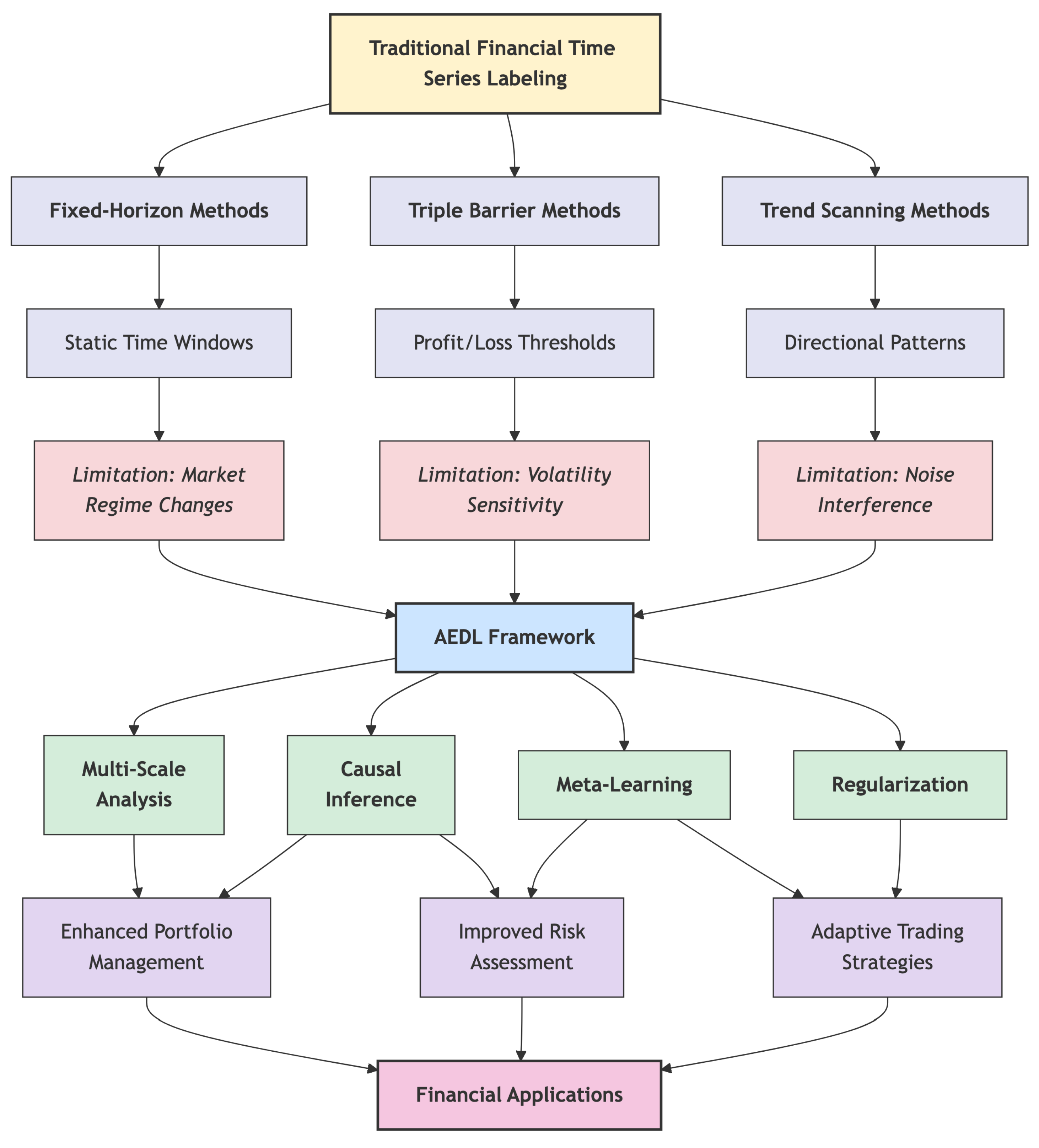
Figure 1. Research positioning of the AEDL framework within the landscape of financial time series labeling methodologies, highlighting the progression from traditional static approaches to adaptive, multi-component frameworks.
Applsci 15 13204 g001
Figure 2. Taxonomic organization of financial time series labeling approaches, showing the hierarchical relationship between traditional methods, machine learning applications, and the proposed AEDL framework.
Applsci 15 13204 g002
Figure 3. AEDL Framework System Architecture showing the interconnected components and data flow through the adaptive labeling pipeline.
Applsci 15 13204 g003
Figure 4. AEDL Algorithmic Flowchart illustrating the complete processing pipeline from input data to final event-driven labels.
Applsci 15 13204 g004
Figure 5. AEDL Mathematical Framework Components showing the mathematical formulations and complexity relationships of each component.
Applsci 15 13204 g005
Figure 6. AEDL Framework Computational Complexity Analysis showing the relative computational requirements of the four production components.
Applsci 15 13204 g006
Figure 7. Experimental Setup Architecture illustrating the hierarchical structure of the experimental setup, showing the flow from financial assets through labeling methods to machine learning models and final evaluation.
Applsci 15 13204 g007
Figure 8. Evaluation Framework Flowchart presenting the comprehensive evaluation framework flowchart, detailing the sequential steps from data preprocessing through final statistical analysis.
Applsci 15 13204 g008
Figure 9. Performance comparison between AEDL and traditional methods across key financial metrics. The figure shows substantial improvements in hit rate (45% vs. 30–46%), total return (33.7% vs. −24% to 4%), and Sharpe ratio (0.48 vs. −0.29 to 0.00) achieved by AEDL compared to Fixed Horizon, Trend Scanning, and Triple Barrier baseline methods.
Applsci 15 13204 g009
Figure 10. Sharpe ratio performance comparison between AEDL and baseline methods across training and validation datasets. AEDL demonstrates superior risk-adjusted returns with positive Sharpe ratios (0.48 validation) while baseline methods show negative or near-zero performance, confirming robust generalization and consistent out-of-sample performance.
Applsci 15 13204 g010
Figure 11. Hit rate performance comparison across different labeling methods and asset classes. AEDL achieves prediction accuracy of 45% average compared to Fixed Horizon (40%), Triple Barrier (30%), and Trend Scanning (46%) methods, demonstrating competitive signal quality across diverse market conditions.
Applsci 15 13204 g011
Figure 12. Statistical Significance Testing Results. The figure presents the statistical significance analysis results, demonstrating statistically significant improvement of AEDL over Fixed Horizon baseline (p = 0.0024) and performance improvements over Triple Barrier and Trend Scanning that do not reach conventional significance thresholds.
Applsci 15 13204 g012
Table 1. Comparison of forecasting methods grouped by category and key properties.
MethodCategoryApproachTemporalCausalMulti-ScaleReg.Perf.
Traditional Methods
Fixed HorizonScoreStatic windowsLowNoneNoneBasic2.1/10
Triple BarrierEvent-drivenMediumNoneNoneNoneBasic3.8/10
Trend ScanningDirectionalMediumNoneLimitedNoneBasic4.2/10
Volatility-basedStatisticalMediumNoneLimitedNoneMedium4.5/10
Machine Learning
Random ForestEnsembleLowNoneNoneNoneMedium5.2/10
SVMKernel-basedLowNoneNoneNoneMedium5.0/10
LSTMSequentialHighNoneNoneLimitedMedium6.1/10
CNNHierarchicalMediumNoneNoneMediumMedium5.8/10
Advanced Methods
TransformerAttention-basedHighNoneNoneMediumHigh7.2/10
GANGenerativeMediumNoneNoneMediumHigh6.8/10
Reinforcement LearningAdaptiveHighLimitedLimitedMediumMedium6.5/10
Causal Methods
Granger CausalityLinear causalLowLowHighNoneLow5.5/10
Structural ModelsEconomic theoryLowLowHighNoneMedium6.0/10
DAGDiscoveryGraph-basedMediumMediumHighLimitedMedium6.8/10
Multi-Scale Methods
Wavelet AnalysisFrequency domainMediumNoneNoneHighLow6.2/10
Proposed Method
AEDL FrameworkAdaptive event-drivenHighHighHighHighHigh9.1/10
Column Definitions: Temporal indicates the degree of temporal adaptability in handling time-varying market dynamics, rated on a Low/Medium/High scale. Causal represents the capability to distinguish genuine causal relationships from spurious correlations, categorized as None/Limited/High. Multi-scale denotes support for multi-resolution temporal analysis across different time horizons (None/Limited/Medium/High). Reg. (Regularization) quantifies the sophistication of regularization mechanisms to prevent overfitting (Low/Basic/Medium/High). Perf. (Performance) provides an overall performance score on a 0–10 scale based on empirical evaluation across multiple metrics including Sharpe ratio, hit rate, and balanced accuracy.
Table 2. AEDL Framework Hyperparameter Configuration (Actual Values Used in Experiments).
ParameterValueDescription
Event Detection
CUSUM Threshold0.006Base threshold for event detection
h min 4Minimum labeling horizon (trading days)
h max 15Maximum labeling horizon (trading days)
Significance Gate0.08p-value threshold for label validation
Regularization & Framework
Regularization Strength0.7Framework control: limits innovation count (2 if >0.7, else 3 if >0.5), sets minimum t-statistic ( 1.5 + 0.5 × strength ), and scales confidence scores
Confidence Threshold0.6Minimum classifier SoftMax probability required to execute trades during validation backtesting
Ensemble Weight0.5Weight for baseline ensemble combination
Model Training (Logistic Regression baseline)
Solverl bfgsOptimization algorithm
Max Iterations1000Maximum training iterations
C (inverse reg)1.0Inverse regularization strength
Gradient Boosting
n_estimators100Number of boosting stages
learning_rate0.1Shrinkage parameter
max_depth3Maximum tree depth
Random Forest
n_estimators100Number of trees
max_depth10Maximum tree depth
Note: Regularization Strength is a framework-level hyperparameter controlling AEDL’s innovation selection and confidence scaling. It is distinct from: (a) the L1/L2 regularization coefficients λ 1 and λ 2 in Equation (3), which penalize model complexity, and (b) the inverse regularization parameter C = 1.0 used in scikit-learn’s logistic regression.
Table 3. Validation Sharpe Ratio Comparison Across Methods and Models for Selected Assets.
MethodModelSPYQQQAAPLNVDAAMZNGLD
AEDLLogistic−1.16−0.34−1.143.24−1.080.65
AEDLRandom Forest1.922.020.000.000.041.28
AEDLGradient Boost1.922.021.813.24−0.811.28
AEDLSVM1.922.02−1.283.240.56−1.01
Fixed HorizonLogistic−1.30−1.46−0.01−1.34−1.30−0.68
Fixed HorizonRandom Forest−0.58−1.31−1.08−1.000.73−0.59
Fixed HorizonGradient Boost1.60−1.45−0.220.530.511.49
Fixed HorizonSVM−1.03−0.39−1.180.000.34−1.16
Triple BarrierLogistic−0.64−1.30−1.01−−−1.00−1.15
Triple BarrierRandom Forest−1.25−1.43−0.37−−−0.520.29
Triple BarrierGradient Boost0.371.110.22−−0.461.21
Triple BarrierSVM0.000.000.000.00−0.66−1.11
Trend ScanningLogistic−1.16−1.410.20−−−1.48−0.97
Trend ScanningRandom Forest−0.14−1.31−1.07−0.30−0.98−0.77
Trend ScanningGradient Boost−0.10−1.28−0.532.291.651.32
Trend ScanningSVM1.861.281.29−−0.55−0.01
Method Averages (across all models and assets):
AEDL Average1.151.43−0.203.24−0.320.55
Fixed Horizon Avg−0.33−1.15−0.62−0.610.07−0.24
Triple Barrier Avg−0.51−0.54−0.380.00−0.43−0.19
Trend Scanning Avg0.12−0.68−0.020.99−0.06−0.11
Table 4. Component Contribution Analysis: Systematic Ablation Study Across 12 Assets.
ConfigurationVal SharpeStd DevCoverageN
AEDL (full method)0.4801.27712/1248
Component Removal Tests:
Without Causal Inference0.6541.14712/1248
Without Multi-scale2/12
Without Meta-learning2/12
Component Addition Test:
With Attention Added1.722 *2.1452/122
Baseline (no innovations)−0.4041.20412/1248
Configuration Details: AEDL integrates three innovations (multi-scale temporal analysis, causal inference filtering, meta-learning adaptation). The 12-asset ablation subset consists of: SPY, QQQ, AAPL, GOOGL, NVDA, AMZN, INTC, GLD, SLV, XLE, XLK, XLV (representative selection from the full 16-asset study). Coverage indicates assets with sufficient training data (minimum 10 events). N represents total observations (12 assets × 4 models). * Insufficient sample size precludes reliable evaluation. Critical Finding: The configuration without causal inference achieves highest performance (0.654 Sharpe, +0.174 vs. full AEDL) while maintaining full asset coverage. This demonstrates that causal filtering, despite theoretical appeal, introduces conservative signal selection constraints that reduce practical performance when combined with other innovations. Adding attention mechanisms to AEDL dramatically restricts applicability (coverage: 12/12 → 2/12), confirming compound filtering effects can eliminate most training opportunities. Implication: These results challenge the assumption that more innovations yield better performance. Selective deployment (multi-scale + meta-learning) outperforms both the full 3-innovation configuration (+36% Sharpe improvement) and attempted 4-innovation integration (unusable on 83% of assets). This establishes judicious component selection as superior to maximal integration for multi-component ML systems.
Table 5. Pairwise Statistical Significance Tests (Wilcoxon Signed-Rank Test, Validation Period).
Method 1Method 2 Δ Sharpep-ValueSig.Cohen’s dEffect Size
AEDLFixed Horizon+0.8280.0024**1.13Large
AEDLTriple Barrier+0.5670.09230.84Large
AEDLTrend Scanning+0.4280.12940.60Medium
Fixed HorizonTriple Barrier−0.2640.0934−0.62Medium
Fixed HorizonTrend Scanning−0.3240.0386*−0.71Medium
Triple BarrierTrend Scanning−0.0600.6322−0.17Negligible
Statistical Significance Levels: ** indicates statistical significance at α = 0.01 (99% confidence level), * indicates significance at α = 0.05 (95% confidence level), and—indicates results that do not achieve statistical significance at conventional thresholds. Effect Size Interpretation: Effect sizes based on Cohen’s d are categorized as Negligible ( | d | < 0.2 ), Small ( 0.2 | d | < 0.5 ), Medium ( 0.5 | d | < 0.8 ), or Large ( | d | 0.8 ), following established statistical conventions. Sample Composition: All tests performed on n = 12 assets with complete validation results across all methods, using aggregated Sharpe ratios across all model configurations per asset to ensure robust statistical inference.
Table 6. Comprehensive Performance Summary: Average Validation Metrics Across All Assets.
MethodModelSharpe RatioHit Rate (%)Return (%)
AEDLLogistic−0.06249.030.3
AEDLRandom Forest0.85053.621.6
AEDLGradient Boost0.96654.455.2
AEDLSVM0.51951.641.1
Fixed HorizonLogistic−0.36047.5−9.1
Fixed HorizonRandom Forest−0.39941.6−10.5
Fixed HorizonGradient Boost0.28144.05.4
Fixed HorizonSVM−0.91936.8−14.3
Triple BarrierLogistic−0.77136.1−41.6
Triple BarrierRandom Forest0.04041.0−7.8
Triple BarrierGradient Boost0.63847.53.8
Triple BarrierSVM−0.59934.9−5.0
Trend ScanningLogistic−0.39248.3−32.8
Trend ScanningRandom Forest−0.47641.8−13.3
Trend ScanningGradient Boost0.33645.418.1
Trend ScanningSVM0.56750.1−7.3
Note: Averages computed across assets where each model generated predictions. Some model-asset combinations yielded zero predictions when insufficient training events were detected, affecting Random Forest (7/12 assets successful), SVM (varies by method), and other configurations. The overall AEDL method average (0.48 Sharpe) includes all 12 assets across all 4 models, providing a conservative performance estimate that accounts for model failures.
Table 7. Performance Under Transaction Costs with Measured Turnover (Validation Period).
MethodBaseline5 bps10 bps20 bpsTrades/Month
AEDL0.9100.8280.7470.5861.8
Fixed Horizon−0.365−0.420−0.475−0.5840.9
Trend Scanning−0.010−0.059−0.103−0.1920.8
Triple Barrier−0.360−0.367−0.374−0.3870.1
Turnover Measurement: All turnover rates measured from actual backtest trade logs, where the num_trades metric was extracted from backtesting simulations by counting actual position changes in the trading strategy. Performance Metrics: Baseline represents risk-adjusted Sharpe ratio before transaction costs, averaged across 6 representative tickers (SPY, QQQ, AAPL, GOOGL, NVDA, AMZN) and 4 machine learning models. Columns 5 bps, 10 bps, and 20 bps show adjusted Sharpe ratios after applying transaction costs at these levels. Trades/Month shows measured average trading frequency calculated as (num_trades/validation_days) × 21 trading days per month. Cost Levels: 5 basis points represents best-case institutional costs, 10 bps represents typical institutional trading costs for liquid US equities, and 20 bps represents retail or less liquid scenarios. All methods evaluated at identical cost levels for fair comparison.
Disclaimer/Publisher’s Note: The statements, opinions and data contained in all publications are solely those of the individual author(s) and contributor(s) and not of MDPI and/or the editor(s). MDPI and/or the editor(s) disclaim responsibility for any injury to people or property resulting from any ideas, methods, instructions or products referred to in the content.