WH-MSDM: A W-Hilbert Curve-Based Multiscale Data Model for Spatial Indexing and Management of 3D Geological Blocks in Digital Earth Applications

Abstract

Multiscale 3D geological characterization and joint analysis are increasingly important topics in spatial information science. However, the non-uniform spatial distribution of objects and scale heterogeneity in geological surveys lead to dispersed storage, long access paths, and limited query performance in managing multiscale 3D geological model data. This study presents a W-Hilbert curve-based multiscale data model (WH-MSDM) that improves data indexing and management through a unified data structure (UDS) for multi-scale blocks and a bidirectional mapping model (BMM) linking spatial coordinates to memory locations. It supports spatial, attribute, hybrid, and cross-scale queries for diverse retrieval tasks. By exploiting the space-filling properties of the W-Hilbert curve to linearize multidimensional geological data into a one-dimensional index, it preserves locality and increases query efficiency across scales. Experimental results on a real 3D geological model demonstrate that WH-MSDM outperforms three mainstream baselines in both unified data organization and diverse query workloads. It thus provides a data-model foundation for Digital Earth-oriented multiscale geological analysis.

1. Introduction

Three-dimensional (3D) geological models integrate structural geometry with physical properties to support the visualization and analysis of subsurface data [1]. They underpin initiatives in Digital Earth [2,3], Smart Cities [4], and Digital Twins [4], and are widely applied to regional resource exploration [5], reservoir characterization [6,7], and tunnel engineering [8,9]. Recent voxel-based geological data models and digital-twin frameworks [10,11] further highlight the importance of unified volumetric representations and efficient voxel storage for large-scale engineering and Earth system applications. In practice, two complementary categories are often distinguished: geological structural models, which express spatial relationships among strata, faults, and rock masses, and geological property models, which consolidate multi-source data into discretized units with attributes such as porosity and mineral composition [12]. Among various representations, block-based models have become mainstream for large-scale 3D geological modeling due to their spatial adaptability and computational efficiency [13]. These models partition the subsurface into 3D cells, each storing geological attributes (e.g., lithology, material properties), typically arranged as structured grids (axis-aligned or stratigraphic-aligned). Such explicit storage enables direct queries and computations (e.g., resource estimation) on the block grid. For instance, Han et al. (2022) [14] developed a three-dimensional engineering geological model for the Xiong’an New Area to support urban planning, and Radwan et al. (2022) [15] employed reservoir modeling to optimize oilfield strategies. However, geological properties vary across scales [16,17], and real-world datasets exhibit uneven spatial density, heterogeneous resolution, and hierarchical block representations, all of which complicate model organization and indexing.

Multiscale partitioning provides a path to reconcile macro-scale navigation with micro-scale analysis. However, effective indexing and management of multiscale blocks are still challenging for three main reasons. First, cross-scale variation is complex, and traditional methods struggle to maintain spatial structure and consistency. This leads to integration issues, information loss, and inefficiency. Second, spatial density is uneven. Uniform partitioning wastes storage in sparse regions and fails to aggregate efficiently in dense regions, which increases access path length. Third, query cost grows with scale dependence because geological features change across scales and require conversion and synchronization steps. Several hierarchical frameworks partially mitigate these issues. Tree-structured indexes and spatial grid coding have been explored [10,18]. Octrees support recursive refinement [19,20] but waste storage in sparse datasets due to empty nodes [21]. VDB variants efficiently manage sparsity [22,23,24], but incur storage overhead in dense regions. Hybrid indexing, such as the TQ-tree-based HiIndex [25], improves visualization but still suffers from high cross-scale mapping cost [26]. Beyond classical octrees and VDB, recent work on hierarchical voxel structures [27] systematically analyzes efficient voxel layouts and access patterns, which further underscores the need for integrated multiscale data models. Space-filling curves transform multi-dimensional data into one-dimensional keys while preserving spatial locality. Among them, Hilbert curves generally provide stronger spatial clustering than Z-order (Morton) codes [28]. From a broader database perspective, WH-MSDM can be viewed as a specialized multidimensional index [29] that leverages W-Hilbert codes to balance locality, storage cost, and query performance in a geological setting. Nevertheless, classical Hilbert curves assume uniform grids and do not encode scale. Consequently, cross-scale clustering is limited, and recursive child-code computation has $O\left(n^2\right)$ complexity [30], which restricts real-time performance in multi-resolution settings.

To alleviate these limitations, Lei et al. (2023) [31] proposed the W-shaped Hilbert curve. The method combines fractal partitioning with optimized child-code computation and maps multi-level n-dimensional blocks into an inverted $2^D$ tree as illustrated in Figure 1. The hierarchical code explicitly embeds scale information and preserves spatial locality. This design enables efficient multiscale operations using bitwise arithmetic. Previous work on the W-Hilbert curve has already provided a systematic comparison against classical Hilbert and Morton curves. Lei et al. (2023) [31] report quantitative locality metrics, visual analyses of clustering patterns, and query benchmarks, and show that W-Hilbert achieves better multiscale spatial clustering and more efficient child-code computation than the classical curves. Building on these results, the present work does not re-evaluate W-Hilbert itself; instead, we treat W-Hilbert as a validated multiscale indexing primitive and focus on designing a unified data structure and bidirectional mapping model that connect these codes to storage layout and application-level queries on 3D geological blocks. Two properties govern the encoding. The initial encoding sets a level-dependent base code given by Equation (1):

$$\begin{array}{cc}\hfill {\mathit{WHcode}}_L^1& =2^{D(L_{max}-L)}-1,\hfill \end{array}$$

(1)

which

ensures distinct base values across levels, where D denotes the spatial dimensionality and $L_{max}$ is the maximum refinement depth. The encoding interval then fixes the intra-level spacing, as given by Equation (2):

$$\begin{array}{cc}\hfill {\delta }_L& =2^{D(L_{max}-L)+1},\hfill \end{array}$$

(2)

which isolates scale levels while allowing for expansion within the same level. In Equation (2), ${\delta }_L$ is the fixed spacing between consecutive W-Hilbert codes at level L, so that all codes at the same level form an evenly spaced sequence. Given block coordinates $C=(x,y,z)$, the standard Hilbert code ${\mathit{Hcode}}_L^i$ at the target level L is first computed. The W-Hilbert code is then obtained as shown in Equation (3), ${\mathit{Hcode}}_L^i$ is the standard Hilbert code at level L, ${\mathit{WHcode}}_L^i$ is the resulting W-Hilbert code, and the two terms respectively encode the intra-level ordering and the level-dependent base code.

$$\begin{array}{c}\hfill {\mathit{WHcode}}_L^i=\underset{\mathrm{Intra}-\mathrm{level}\mathrm{offset}}{\underbrace{{\mathit{Hcode}}_L^i·2^{D(L_{max}-L)+1}}}+\underset{\mathrm{Base}\mathrm{code}}{\underbrace{2^{D(L_{max}-L)}-1}}.\end{array}$$

(3)

In this expression, the first term ${\mathit{Hcode}}_L^i·2^{D(L_{max}-L)+1}$ preserves the spatial ordering of the Hilbert code within level L the second term $2^{D(L_{max}-L)}-1$ anchors the code to the scale hierarchy.

Decoding proceeds in two steps. The scale level L is inferred from the trailing bits of the binary form, which can be written as shown in Equation (4):

$$\begin{array}{c}\hfill {\mathit{WHcode}}_L^i\equiv {\left(\underset{len{\left(i\right)}_2}{\underbrace{**\dots *}}|0\underset{D(L_{max}-L)}{\underbrace{1\dots 1}}\right)}_2.\end{array}$$

(4)

so that counting the consecutive trailing 1s yields

$$\begin{array}{c}\hfill L=L_{max}-{\displaystyle \frac{\mathrm{Trailing}1’\mathrm{s}\mathrm{count}}{D}}.\end{array}$$

(5)

Here the “Trailing 1’s count” denotes the number of consecutive 1 bits at the end of the binary representation of ${\mathit{WHcode}}_L^i$, which uniquely determines the scale level L according to the pattern in Equation (4). The intra-level Hilbert code is then recovered by

$$\begin{array}{c}\hfill {Hcode}_L^i={\displaystyle \frac{{\mathit{WHcode}}_L^i-(2^{D(L_{max}-L)}-1)}{2^{D(L_{max}-L)+1}}},\end{array}$$

(6)

The intra-level Hilbert code is then recovered by  (6), and standard Hilbert decoding maps ${\mathit{Hcode}}_L^i$ back to spatial coordinates [30]. Taken together, Equations (4)–(6) show that level information and the standard Hilbert index can be recovered from a single W-Hilbert code using simple arithmetic and bit operations. In summary, W-Hilbert improves cross-scale spatial locality and the efficiency of encoding and decoding. Given the base and interval in Equations (1) and (2) and the decoding in Equations (4)–(6), W-Hilbert yields a hierarchical code space with explicit scale markers and strong spatial locality, which we adopt as the backbone for coding multi-resolution blocks. What remains unmet in practice is the need for an integrated model to bind these codes to storage for attribute-rich blocks and to provide spatial, attributive, hybrid, and cross-scale query operators with predictable cost, thereby connecting W-Hilbert’s cross-scale locality with end-to-end storage, indexing, and querying on hierarchical block models.

To fill this gap, we propose WH-MSDM, a comprehensive multiscale data model that elevates W-Hilbert encoding into a complete data management solution. WH-MSDM introduces a unified data structure (UDS) that assigns contiguous W-Hilbert codes to blocks at every resolution, enabling single-pass retrieval without redundant storage, and a bidirectional mapping model (BMM) that binds 3D block coordinates to these codes for unified hierarchical indexing. Building on this foundation, we design scalable query algorithms, including spatial, attributive, hybrid, and cross-scale queries, which exploit the WH-MSDM framework to retrieve multi-resolution block data flexibly and precisely. This framework provides an integrated solution that unifies storage, indexing, and querying for multiscale 3D geological data, which provides a data-model foundation for Digital Earth-oriented multiscale 3D geological analysis.

2. Materials and Methods

WH-MSDM provides a practical approach to handling complex, multiscale spatial data through Unified Data Structure (UDS), Bidirectional Mapping Model (BMM), and specialized query algorithms.

2.1. Unified Data Structure

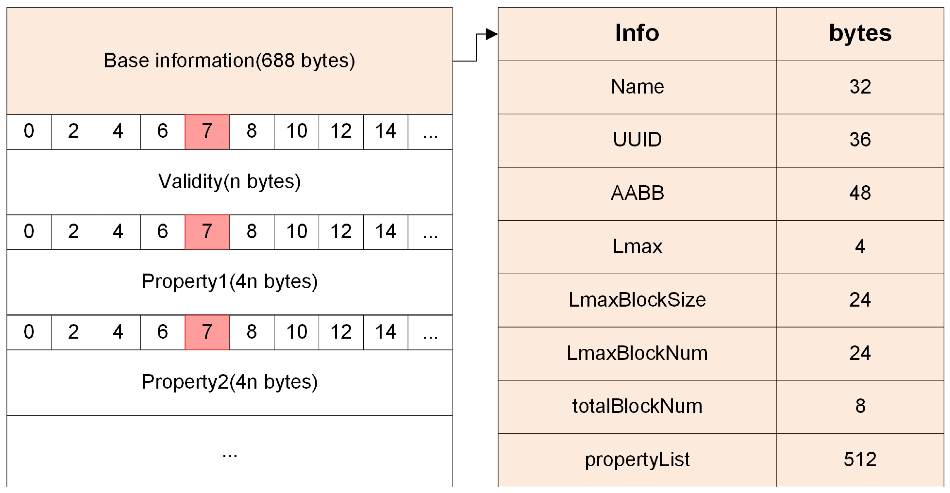
The UDS is a 3D structure that integrates spatial and attribute information of geological objects, as shown in Figure 2. It has three main components: basic information, validity flags, and attribute data. Basic information includes the model’s name (Name), unique ID (UUID), bounding box (AABB), max detail level ($L_{max}$), total block counts $N={\sum }_{l=0}^{L_{max}}{\left(N_L\right)}^D$, and property list. Validity flags (T for valid and F for invalid) indicate whether blocks accurately represent geological structures. The attribute section organizes similar attributes together for efficient data management and retrieval.

2.2. Bidirectional Mapping Model

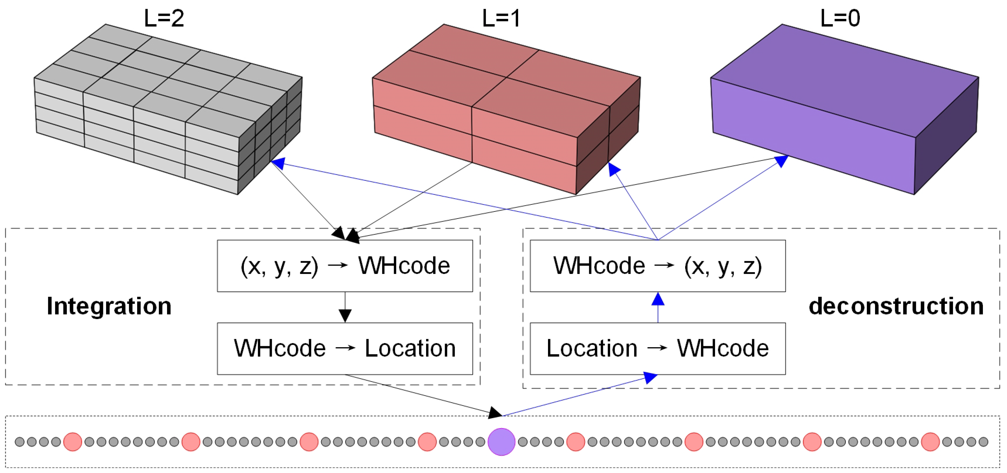
Figure 3 shows the bidirectional mapping model (BMM) of WH-MSDM, which involves integration and deconstruction. The integration process combines 3D coordinates into a unified W-Hilbert code, mapping spatial coordinates and scale levels of blocks to UDS positions, creating a multiscale model. The deconstruction reverses this by mapping UDS positions back to spatial coordinates and scale levels, decoding the W-Hilbert code to retrieve the coordinates.

2.2.1. The Integration Process

The integration process in BMM involves W-Hilbert encoding [31] (Section 1) and memory location mapping so that multiscale blocks are placed contiguously in the UDS.

Memory location mapping. W-Hilbert encoding converts three-dimensional block coordinates into a level-aware linear order that preserves spatial locality. Based on the W-Hilbert curve, coordinate encoding projects multiscale block models to a one-dimensional key space, and location mapping assigns each key to a memory position in the UDS while preserving spatial information and the linear order.

Step 1: Obtain and integrate the basic information of the block models at all scales to construct the UDS.

Step 2: Given the maximum level $L_{max}$, the current level L, and the dimension D, determine the initial block code ${\mathit{WHcode}}_L^1$ and the intra-level spacing ${\delta }_L$ using Equations (1) and (2).

Step 3: For any level L and the $i_{th}$ block at that level, compute the cumulative count of blocks whose encoding values do not exceed ${\mathit{WHcode}}_L^i$. Here, ${\mathit{Num}}_L^i$ denotes the cumulative number of blocks at level L whose W-Hilbert codes are less than or equal to ${\mathit{WHcode}}_L^i$, including the current block, and ${\delta }_L$ is the code interval defined in Equation (2).

$$\begin{array}{c}\hfill {\mathit{Num}}_L^i=({\mathit{WHcode}}_L^i-{\mathit{WHcode}}_L^1)/{\delta }_L+1.\end{array}$$

(7)

Step 4: Accumulate the totals over all levels to determine the global position of the current block in the UDS.

$$\begin{array}{c}\hfill \mathit{loc}=\sum _{L=0}^{L_{max}}{Num}_L^i-1=\sum _{L=0}^{L_{max}}\left(\left({\mathit{WHcode}}_L^i-{\mathit{WHcode}}_L^1\right)/{\delta }_L+1\right)-1.\end{array}$$

(8)

This yields a zero-based linear index for each block and establishes a one-to-one correspondence between hierarchical blocks and memory locations in the UDS, which preserves spatial locality and supports multiscale access. In this formulation, loc is the global index of the block in the UDS obtained by summing the per-level cumulative counts ${\mathit{Num}}_L^i$ over all levels.

2.2.2. The Deconstruction Process

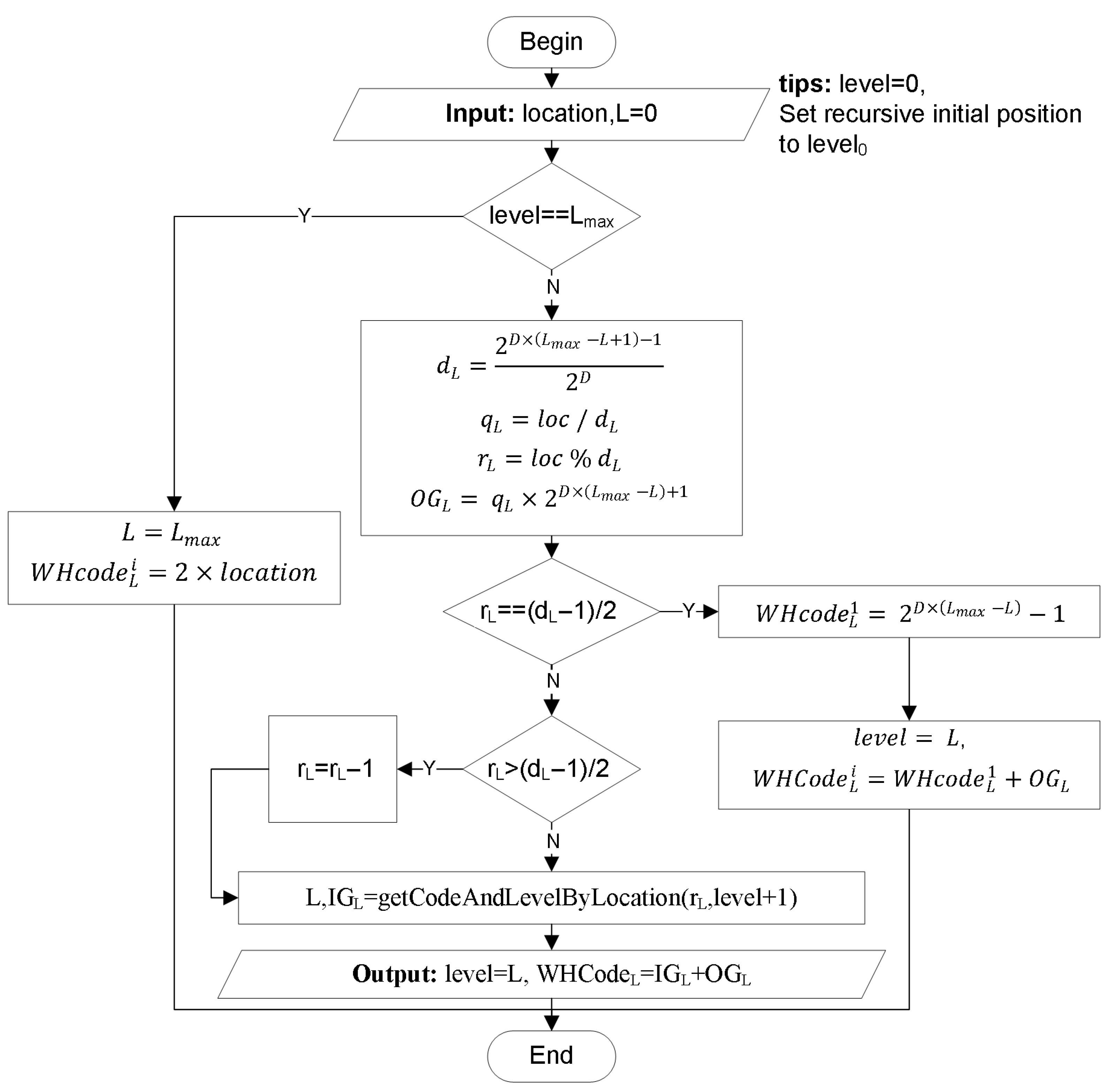
Deconstruction reverses integration by mapping a global UDS position back to the scale level, the W-Hilbert code, and finally the spatial coordinates. Figure 3 and Figure 4 outline this reverse mapping: the scale level is identified, the corresponding W-Hilbert code is recovered, and standard decoding produces the block coordinates. To make the reverse mapping local and efficient, the notion of group is introduced to formalize external offsets and intra-group re-encoding within the BMM.

Definition 1

(Group). At scale level L, a block encoded as ${\mathit{WHcode}}_L^i$ together with all of its descendants at finer levels forms a group, denoted as ${\mathit{Group}}_L^{{\mathit{WHcode}}_L^i}$.

Definition 2

(Current group). A block with encoding ${\mathit{WHcode}}_L^i$ belongs to a unique group at level L. This constituent group is denoted ${\mathit{CGroup}}_L^{{\mathit{WHcode}}_L^i}$.

Definition 3

(Left sibling group). Let ${\mathit{CGroup}}_L^{{\mathit{WHcode}}_L^i}$ be the current group of a block at level L. The left sibling group, denoted as ${\mathit{LBGroup}}_L^{{\mathit{WHcode}}_L^i}$, consists of all groups at level L that share the same parent and lie strictly to its left on the W-Hilbert order. All blocks at level 0 are siblings, whereas those without a common parent are not.

Definition 4

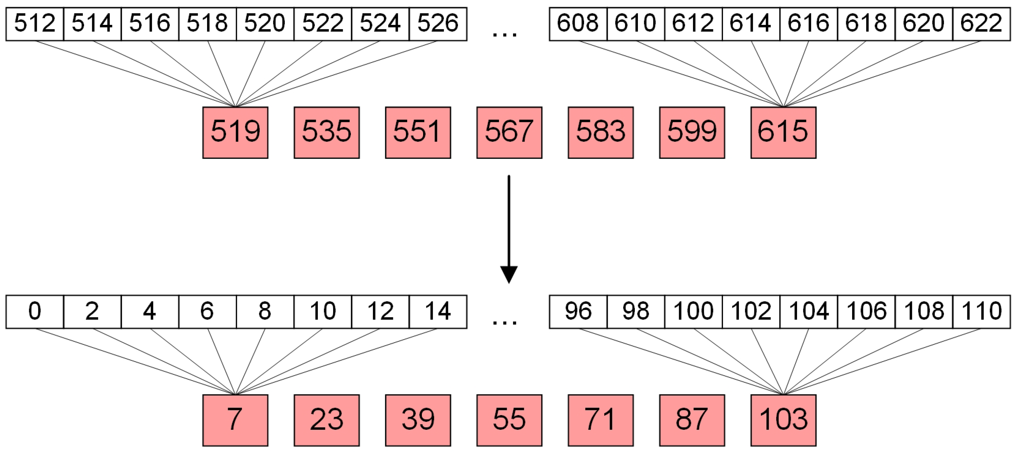
(Current group encoding). Within ${\mathit{CGroup}}_L^{{\mathit{WHcode}}_L^i}$, blocks are re-encoded from 0 after subtracting external offsets. The resulting intra-group code of the current block is called the current group encoding and is denoted ${\mathit{CGCode}}_L^{{\mathit{WHcode}}_L^i}$. An example is shown in Figure 5.

Definition 5

(Left sibling group encoding). For a block with encoding ${\mathit{WHcode}}_L^i$, the left sibling group ${\mathit{LBGroup}}_L^{{\mathit{WHcode}}_L^i}$ is re-encoded from 0. The left sibling group encoding, denoted ${\mathit{LBCode}}_L^{{\mathit{WHcode}}_{L^{\prime }}^i}$, is defined as the maximum intra-group code over ${\mathit{LBGroup}}_L^{{\mathit{WHcode}}_L^i}$ plus 2. An example is shown in Figure 6.

The deconstruction pipeline consists of three parts: group external encoding, group internal encoding, and W-Hilbert decoding (see Section 1). Figure 7 summarizes the end-to-end procedure.

Calculating group external encoding. Group external encoding aggregates the encodings of all completed groups to the left of the current group and yields the external offset on the space-filling curve. The calculation proceeds as follows.

Step 1: Compute the number of blocks per group at level L.

$$\begin{array}{cc}\hfill d_L& =\sum _{l=0}^{L_{max}-L}{2}^{D\times l}\hfill \\ \hfill & ={\displaystyle \frac{2^{D\times (L_{max}-L+1)}-1}{2^D-1}}.\hfill \end{array}$$

(9)

Here $d_L$ is the total number of blocks contained in a single group at level L when all descendant levels from L to $L_{max}$ are included.

Step 2: Determine the number of completed groups preceding the current block by integer division of the global location:

$$\begin{array}{c}\hfill q_L=loc/d_L.\end{array}$$

(10)

The integer $q_L$ counts how many complete groups at level L precede the current block along the W-Hilbert curve; it is obtained by integer division of the global index loc by the group size $d_L$.

Step 3: According to the W-Hilbert rules, the code span occupied by any group equals twice the number of finest-level blocks within that group:

$$\begin{array}{c}\hfill {\mathit{occupy}}_L=2^{D\times (L_{max}-L)+1}.\end{array}$$

(11)

The quantity ${\mathit{occupy}}_L$ is the span, in W-Hilbert code space, occupied by any single group at level L, which is twice the number of finest-level blocks within that group.

Step 4: The maximum external encoding consumed by all preceding groups at level L is then

$$\begin{array}{c}\hfill {\mathit{OG}}_L=q_l\times {\mathit{occupy}}_L.\end{array}$$

(12)

Calculating group internal encoding. Group internal encoding gives the W-Hilbert position of the current block within its own group, independent of external offsets.

Step 1: Compute the position of the current block within its group:

$$\begin{array}{c}\hfill r_L=\mathit{loc}\%d_L.\end{array}$$

(13)

Step 2: Test whether the block coincides with the group root at level L. Let

$$\begin{array}{c}\hfill \mathit{pos}=(d_L-1)/2.\end{array}$$

(14)

In this context, $r_L$ is the position of the current block within its group (0-based), pos denotes the index of the group root at level L, and $I{G}_L$ and $I{G}_{L+1}$ (defined below) denote the intra-group encoding contributions from levels L and $L+1$, respectively. If $r_L$ equals pos, the intra-group encoding equals ${WHcode}_L^1$. If $r_L$ is greater than pos, decrement $r_L$ by one to exclude the parent when descending to the next level.

Step 3: Propagate the intra-group position to the next level via

$$\begin{array}{c}\hfill {\mathit{IG}}_L={\mathit{OG}}_{L+1}+{\mathit{IG}}_{L+1}.\end{array}$$

(15)

Step 4: Continue the recursion until the maximum level $L_{max}$, where the W-Hilbert encoding interval equals 2, yielding

$$\begin{array}{c}\hfill {\mathit{IG}}_{max}=2\times L_{max}.\end{array}$$

(16)

The W-Hilbert code for the current block is obtained by combining the external offset ${\mathit{OG}}_L$ with the intra-group term ${\mathit{IG}}_L$. The spatial coordinates are then recovered by applying W-Hilbert decoding, which completes the reverse mapping from a global UDS position to geometry.

2.2.3. Data Integration Process

WH-MSDM defines a unified spatial grid framework that integrates multiscale data from heterogeneous sources into a single global indexing structure. Data at each scale are first partitioned into spatial blocks. For each block, a block-level index and associated metadata are generated to record its spatial extent, resolution, and data source. A validity flag is then assigned so that blocks identified as empty or redundant can be excluded from the working set, ensuring that only blocks containing valid data participate in subsequent integration. To preserve global coherence, however, the spatial identifiers of all blocks, including those that are filtered out, are retained in order to maintain the overall spatial distribution. In the next stage, the multi-dimensional coordinates of each block are mapped to a one-dimensional sequence using a W-Hilbert space-filling curve, which preserves spatial adjacency. Blocks are then ordered by their Hilbert indices, allowing spatial locality to be exploited and improving access efficiency during integration.

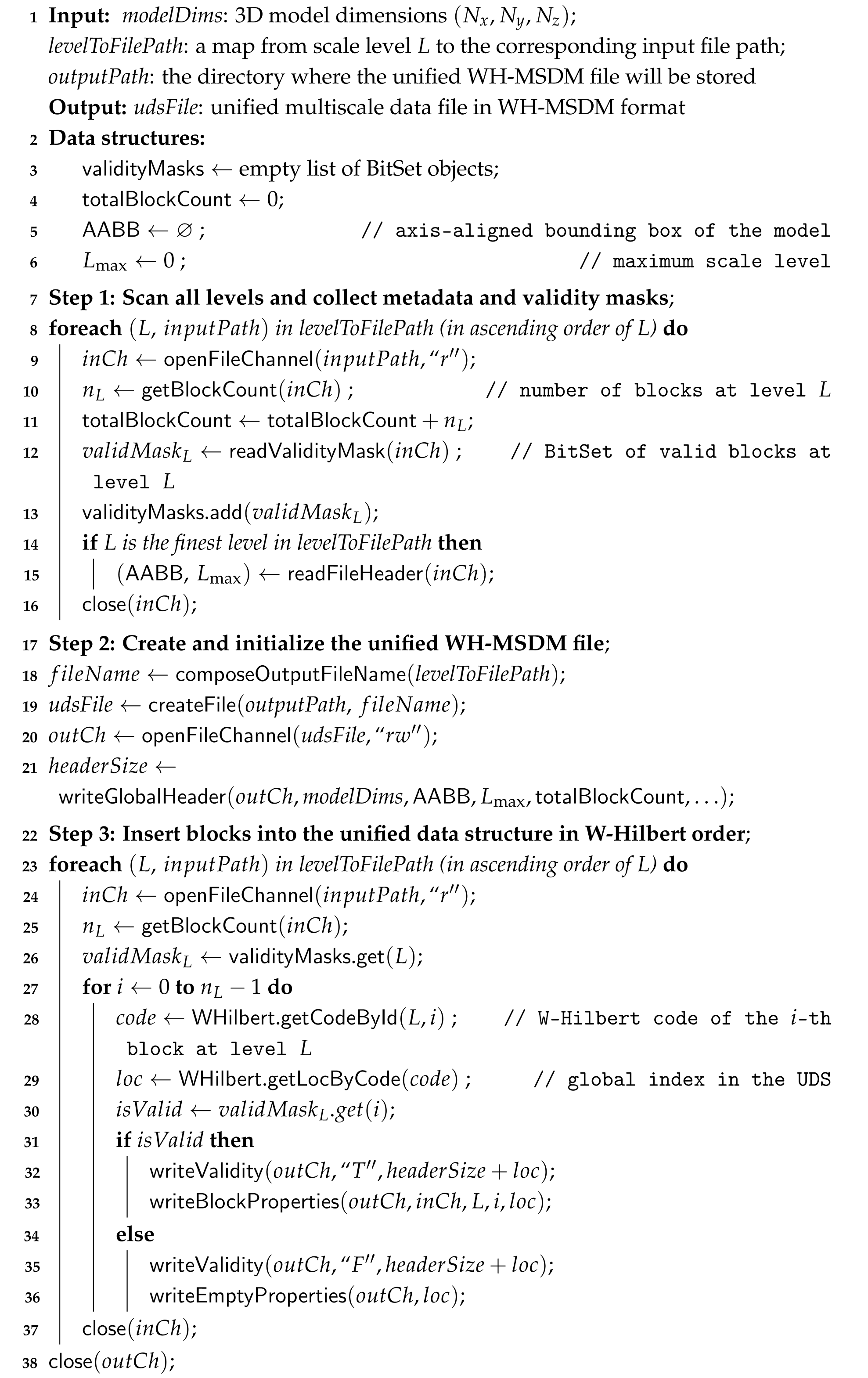
To operationalize this framework, a two-stage W-Hilbert-based coding and mapping procedure is developed to populate the UDS from raw file sources, as summarized in Algorithm 1. The algorithm first initializes the object dimensions, block validity flags, and block counters (lines 3–6), and then traverses the input file paths to update block counts and collect validity information (lines 8–13). At the maximum level, it records the model’s metadata (lines 10–11), creates the target file, and writes the file header (lines 18–21). In the second pass, the algorithm re-traverses the file paths to compute W-Hilbert codes and the corresponding UDS positions for each block (lines 23–30). Valid blocks and their attributes are then written into the target file, while invalid blocks are represented by zero entries (lines 31–36). The resulting file is a compact, globally indexed multiscale block model that is well organized for downstream querying and analysis.

Algorithm 1: Unified organization of multiscale blocks into WH-MSDM

2.3. Diverse Query Algorithms

Given a query condition C, a query operation Q is applied on block data B in the UDS to obtain a block set R that satisfies the specified application requirements. Under this abstraction, Q operates on C to produce the corresponding subset of blocks, which can be written as $R=Q\left(C\right)=\left\{B\right|B\in \mathit{UDS},BsatisfiesC\}$. In this work, Q covers four query types: spatial ($Q_S$), attribute ($Q_A$), hybrid ($Q_H$) and cross-scale ($Q_C$) queries.

2.3.1. Spatial Query ($Q_S$)

Spatial querying within multiscale blocks supports the identification of data based on spatial locations or ranges. The process begins by uniformly partitioning the query region into grid cells at multiple spatial resolution levels, from coarse to fine. Bit-shift operations are then applied to transform the minimum and maximum query coordinates into block index intervals for the current resolution level. For each level, the algorithm iterates over all 3D grid cells within the corresponding interval and generates a one-dimensional spatial code for each cell using a W-Hilbert space-filling curve, thereby preserving spatial locality. These codes are used to locate the corresponding data blocks in the multiscale block management structure (MSBM), where block validity is checked and the attribute values of valid blocks are retrieved under a predefined list of attribute names. The retrieved attributes are finally aggregated across all resolution levels for the spatial region of interest, which enables flexible queries over arbitrary spatial extents.

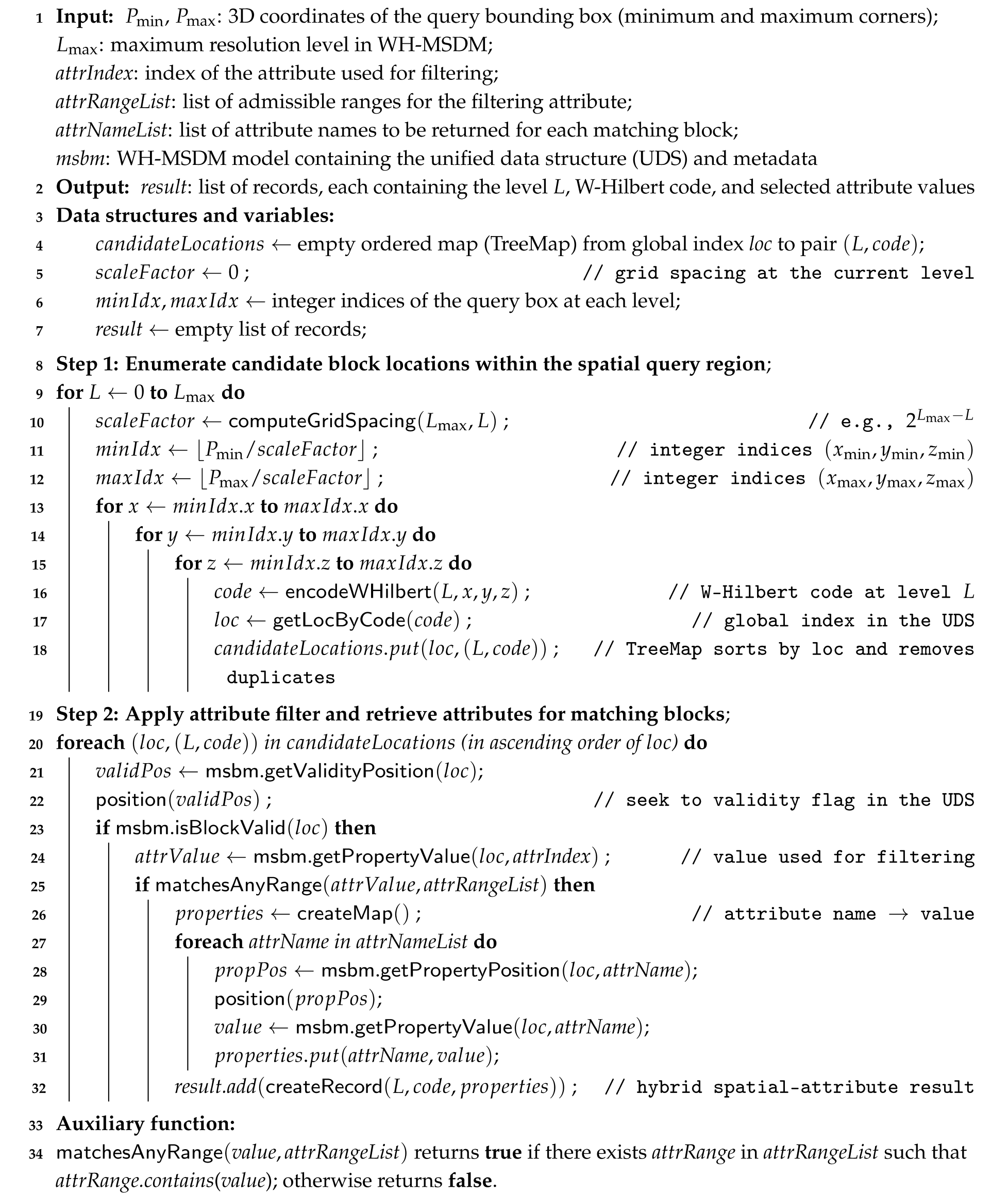
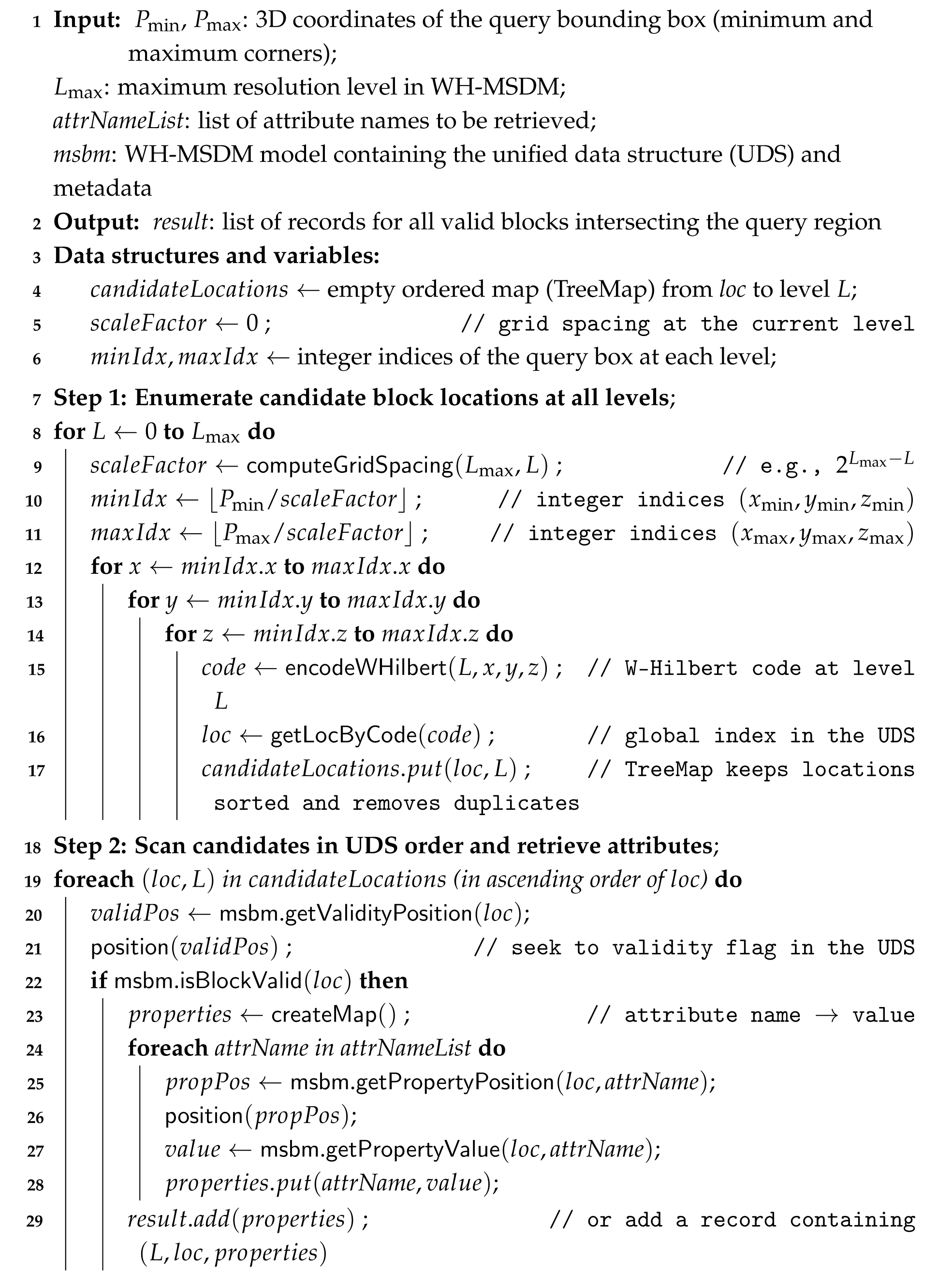
To implement this procedure efficiently on the UDS, we combine W-Hilbert coding with a TreeMap-based index, as summarized in Algorithm 2. Block coordinates are mapped to W-Hilbert codes and converted to UDS positions. The resulting location set is organized in a TreeMap, where the key is the block location and the value stores the W-Hilbert code along with the scale hierarchy L. The underlying red-black tree maintains the entries in sorted order, exploiting the spatial continuity of the W-Hilbert curve to support efficient retrieval and reduce I/O overhead. Given the diagonal endpoints $P_{min}$ and $P_{max}$, the algorithm first instantiates the TreeMap (line 4–6), then iterates over each scale hierarchy to compute the coordinate interval for the current level (lines 8–11). It traverses all combinations of x, y, and z within this interval, generates positional codes with W-Hilbert coding, and inserts them into the TreeMap (lines 12–17). For each stored position, it verifies the existence and validity of the corresponding block in the MSBM (lines 19–21). Valid blocks are then recorded in a HashMap together with their attribute values (lines 22–28), and these attributes are incorporated into the final query result (line 29).

2.3.2. Attribute Query ($Q_A$)

The algorithm operates on the multiscale block management structure (MSBM) to jointly filter target blocks by spatial range and attribute constraints. It first partitions the query region into grid cells at multiple resolution levels, beginning with coarse cells for broad coverage and progressively refining with smaller cells. For each cell, it computes a one-dimensional spatial code from the two- or three-dimensional coordinates in a locality-preserving manner (for example, via W-Hilbert coding), which enables rapid matching against the MSBM index. Each matched candidate is then validated for spatial relevance by discarding empty blocks and blocks outside the target region. Attribute filtering follows: for every block that passes spatial validation, the algorithm retrieves the requested attributes and evaluates them against the specified predicates, such as numeric ranges or text matches. Only blocks that satisfy both spatial validity and attribute conditions are retained. Finally, the algorithm aggregates and outputs the codes of all qualifying blocks by resolution level, listing coarse-level results before fine-level results so that users can inspect outcomes from macro to micro scales in support of subsequent multiscale analysis or visualization.

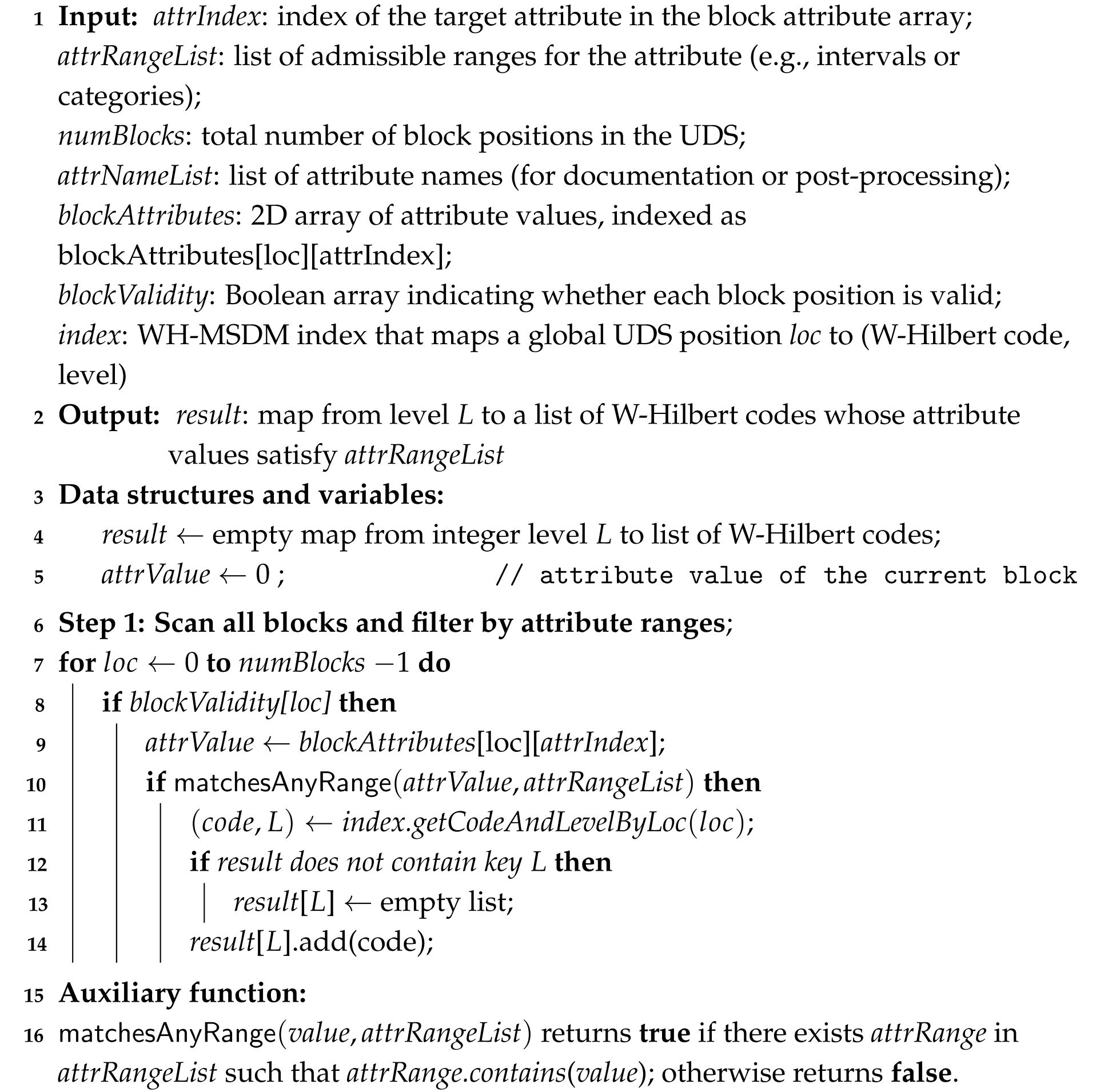
When attribute conditions are the primary driver, the procedure specializes while preserving the same multiscale output format. Attribute queries filter blocks by lithology or mineral grade, first screening attribute values and then locating the corresponding spatial blocks in the MSBM. In Algorithm 3, the result containers are initialized (line 3–5), valid blocks are scanned to evaluate attribute predicates and collect matching blocks’ codes together with their scale hierarchy (lines 7 to 14), and the algorithm outputs a list of block codes sorted by scale level.

Algorithm 2: Multiscale spatial range query based on WH-MSDM ($Q_S$)

Algorithm 3: Multiscale attribute query based on WH-MSDM ($Q_A$)

2.3.3. Hybrid Query (Q_H)

The core of the method is the coordinated use of spatial range filtering and attributebased selection under a multiscale grid encoding. At each resolution level, the input minimum and maximum coordinates are scaled to delineate the three-dimensional gridcell range to be examined. For every grid cell in this range, it then computes a onedimensional W-Hilbert code from the two- or three-dimensional coordinates and records the corresponding position in the global data structure (UDS), together with its scale level, in an ordered map (TreeMap). This structure preserves spatial locality while organizing candidate blocks by their locations and scales. The algorithm next iterates over these candidates and uses the WH-MSDM index to check each block’s validity flag, discarding blocks that are empty or invalid. For every valid block, it retrieves the stored attribute values and compares them with the user-specified attribute ranges. Once an attribute is found to lie within a required range, the block’s code and scale level are added to the resultset, and attribute checking for that block terminates.

To implement this hybrid query strategy in practice, the procedure builds on the spatial query stage and then incorporates attribute filtering, as summarized in Algorithm 4. The algorithm begins by initializing a TreeMap to store valid block positions and their scale levels (lines 3–7), and then traverses each scale hierarchy to compute the coordinate ranges for the current level (lines 9–12). For every block within these ranges, it computes the W-Hilbert encoding, converts it to a UDS position, and inserts the position, code, and scale level into the TreeMap (lines 20–26). In the final stage, it iterates through the TreeMap entries to check block validity in WH-MSDM and to evaluate the corresponding attribute values against the query conditions, adding the encodings of all matching blocks to the result set (lines 27–32). By performing spatial filtering before attribute evaluation, proceeding from coarse to acceptable resolutions, and utilizing Hilbert encoding to maintain data locality, the algorithm enables the rapid retrieval of blocks that satisfy multiple attribute constraints within arbitrary spatial regions of a large three-dimensional grid model.

Algorithm 4: Multiscale hybrid query based on WH-MSDM (QH)

2.3.4. Cross-Scale Query ($Q_C$)

We first introduce two key theorems that characterize the behavior of W-Hilbert codes across scales and form the theoretical basis for the cross-scale query algorithms. Intuitively, cross-scale queries in WH-MSDM treat a block and all of its descendants as a contiguous interval on the W-Hilbert curve. If the encoding has this property, then parent–child queries can be implemented by simple interval computations rather than by traversing an explicit tree. The two theorems below formalize this behavior. Theorem 1 shows that the distance, in code space, between a parent code and the minimum (or maximum) code of its descendants depends only on the scale level and is equal to the first code at that level. Theorem 2 shows that the binary representations of a parent code and any of its descendants share a common prefix and differ only in the lowest bits that correspond to finer scales. Together, these properties guarantee that all descendants of a block form a compact, easy-to-enumerate interval on the W-Hilbert curve.

Theorem 1

(Encoding offset). At scale level L, the coding offset ${\mathit{offset}}_L$ between a block’s W-Hilbert code and the smallest (or largest) W-Hilbert code of its sub-blocks equals the first coding value ${\mathit{WHcode}}_L^1$ of that level.

Proof of Theorem 1 .

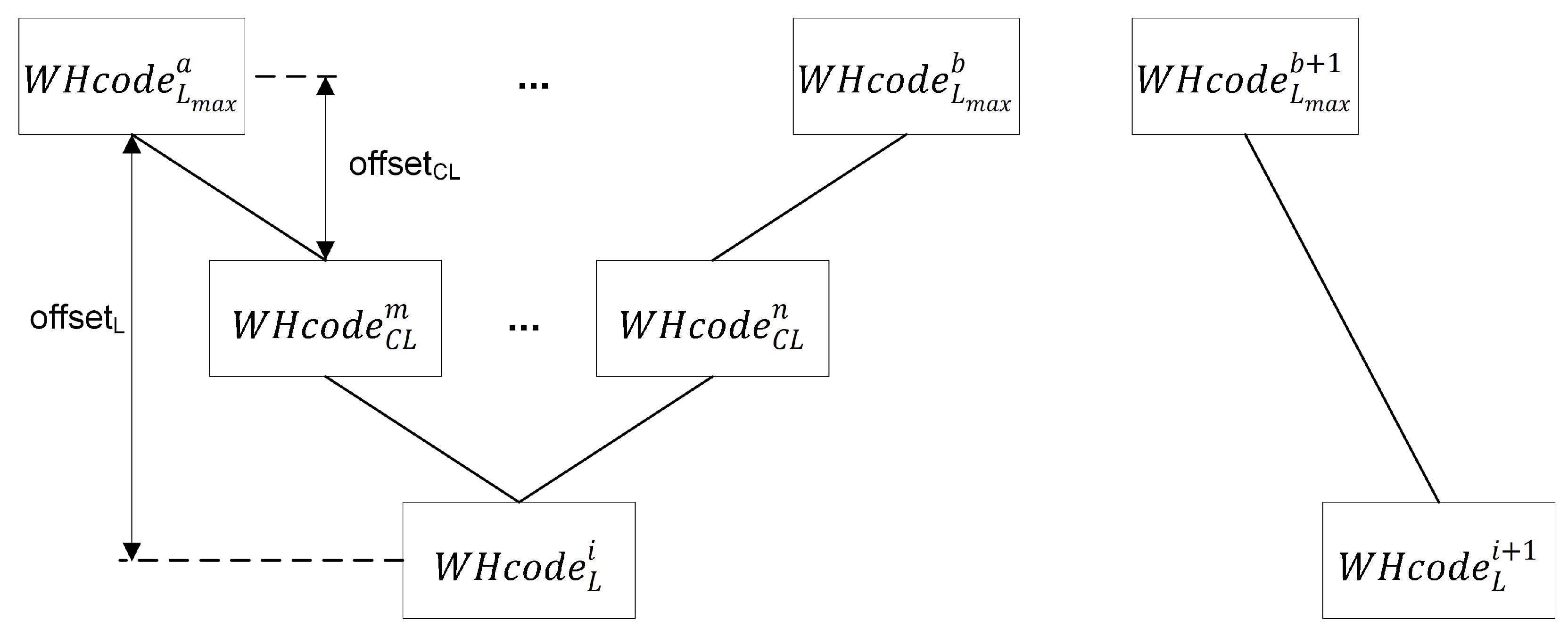
Let ${\mathit{WHcode}}_L^i$ and ${\mathit{WHcode}}_L^{i+1}$ be adjacent blocks at level L. The minimum and maximum block codes of ${\mathit{WHcode}}_L^i$ in the $L_{max}$ are denoted by ${\mathit{WHcode}}_L^a$ and ${\mathit{WHcode}}_L^b$, while the minimum block code of ${\mathit{WHcode}}_L^{i+1}$ are denoted by ${\mathit{WHcode}}_L^{b+1}$. Figure 8 shows the scale hierarchy relationship. The offset between ${\mathit{WHcode}}_L^i$ and its smallest sub-block code ${\mathit{WHcode}}_{L_{max}}^a$ is

$$\begin{array}{c}\hfill {\mathit{offset}}_L={\mathit{WHcode}}_L^i-{\mathit{WHcode}}_{L_{max}}^a.\end{array}$$

(17)

By the even-coding property of the W-Hilbert curve at the maximal level $L_{max}$,

$$\begin{array}{c}\hfill {\mathit{WHcode}}_L^b-{\mathit{WHcode}}_{L_{max}}^a=2\times {\mathit{offset}}_L.\end{array}$$

(18)

Substituting Equations (17) and (18) into Equation (2) gives

$$\begin{array}{cc}\hfill {\delta }_L& ={\mathit{WHcode}}_L^{i+1}-{\mathit{WHcode}}_L^i\hfill \\ \hfill & =2\times {\mathit{offset}}_L+{\delta }_{L_{max}}.\hfill \end{array}$$

(19)

Rearranging Equation (19) yields

$$\begin{array}{cc}\hfill {\mathit{offset}}_L& ={\displaystyle \frac{{\delta }_L-{\delta }_{L_{max}}}{2}}\hfill \\ \hfill & =2^{D\times (L_{max}-L)}-1,\hfill \end{array}$$

(20)

which proves that ${\mathit{offset}}_L={\mathit{WHcode}}_L^1$. In other words, the smallest and largest of all descendants of ${\mathit{WHcode}}_L^i$ are obtained by subtracting and adding ${\mathit{WHcode}}_L^1$, respectively. The value ${\mathit{WHcode}}_L^1$ depends only on the level L and the spatial dimension D, so the offset between a parent block and the block interval spanned by all of its descendants is independent of the particular position of the block on the curve. This level-dependent offset is the key to computing child-code ranges for cross-scale queries without explicit tree traversal.

□

Theorem 2

(Encoding differences). For any block code ${\mathit{WHcode}}_L^i$ with $L<L_{max}$, the binary representation of ${\mathit{WHcode}}_L^i$ and that of any of its W-Hilbert sub-blocks differ only in the lowest $D\times (L_{max}-L)+1$ bits.

Proof of Theorem 2 .

By Equation (4), the first code ${\mathit{WHcode}}_L^1$ at level L occupies $D\times (L_{max}-L)+1$ bits in binary. Theorem 1 indicates that the sub-block code range within ${\mathit{WHcode}}_L^i$ is $[{\mathit{WHcode}}_L^i-{\mathit{WHcode}}_L^1,{\mathit{WHcode}}_L^i+{\mathit{WHcode}}_L^1]$. The binary forms of the range endpoints are

$$\begin{array}{cc}\hfill {\left({\mathit{WHcode}}_L^i-{\mathit{WHcode}}_L^1\right)}_2& ={\left(X\dots X0 \underset{D\times (L_{max}-L)}{\underbrace{111\dots 111}}\right)}_2-{\left(0 \underset{D\times (L_{max}-L)}{\underbrace{111\dots 111}}\right)}_2\hfill \\ \hfill & ={\left(X\dots X\underset{D\times (L_{max}-L)+1}{\underbrace{000\dots 000}}\right)}_2,\hfill \end{array}$$

(21)

$$\begin{array}{cc}\hfill {\left({\mathit{WHcode}}_L^i+{\mathit{WHcode}}_L^1\right)}_2& ={\left(X\dots X0 \underset{D\times (L_{max}-L)}{\underbrace{111\dots 111}}\right)}_2+{\left(0 \underset{D\times (L_{max}-L)}{\underbrace{111\dots 111}}\right)}_2\hfill \\ \hfill & ={\left(X\dots X \underset{D\times (L_{max}-L)}{\underbrace{111\dots 111}} 0\right)}_2.\hfill \end{array}$$

(22)

Equations (21) and (22) show that only the lowest $D\times (L_{max}-L)+1$ bits vary among all sub-blocks encoded under ${\mathit{WHcode}}_L^i$. These low-order bits encode the finer-scale refinements of the block. Therefore, all descendant codes lie inside a contiguous interval in which the upper bits are fixed to the parent code and only the lower bits vary. This structure allows us to express the complete set of descendant codes as a union of arithmetic progressions with stride ${\delta }_{C}L$ at each level $CL$, as used in the child-block query algorithm. From an implementation perspective, Theorem 2 justifies using simple bit masks and additions to enumerate descendants, rather than recursive descent along a tree. □

This property directly supports cross-scale queries. A child-block query for a given ${\mathit{WHcode}}_L^i$ enumerates all descendants at levels CL with $L\le \mathit{CL}\le L_{max}$, while a parent-block query enumerates ancestors at levels PL with $0\le \mathit{PL}\le L$.

Child Blocks Query ($Q_{CC}$)

Given an arbitrary block ${\mathit{WHcode}}_L^i$, the goal of the child-block query is to enumerate all its descendants across finer scale levels. To achieve this, we first determine the child-code boundary range at each target scale level CL. As shown in Figure 8 and implied by Theorem 1, the child block coding interval $[{\mathit{WHcode}}_{CL}^m,{\mathit{WHcode}}_{CL}^n]$ at any scale level CL with $L\le \mathit{CL}\le L_{max}$ can be written as

$$\begin{array}{cc}\hfill {\mathit{WHcode}}_{CL}^m& ={\mathit{WHcode}}_{L_{max}}^a+{\mathit{offset}}_{CL}\hfill \\ \hfill & ={\mathit{WHcode}}_L^i-{\mathit{WHcode}}_L^1+{\mathit{WHcode}}_{CL}^1,\hfill \end{array}$$

(23)

$${\mathit{WHcode}}_{CL}^n={\mathit{WHcode}}_L^i+{\mathit{WHcode}}_L^1-{\mathit{WHcode}}_{CL}^1.$$

(24)

These expressions provide closed-form lower and upper bounds for the child codes of ${\mathit{WHcode}}_L^i$ at level CL. Finally, the code increment ${\delta }_{CL}$ at level CL is obtained from Equation (2), and all child blocks at that level are enumerated by stepping through the interval $[{\mathit{WHcode}}_{CL}^m,{\mathit{WHcode}}_{CL}^n]$ with stride ${\delta }_{CL}$. By merging the code sets collected over all CL from L to $L_{max}$, we obtain the complete set of child blocks for ${\mathit{WHcode}}_L^i$.

Parent Block Query ($Q_{CP}$)

Complementary to the child-block query, the parent-block query lifts a given block to a coarser scale via W-Hilbert decoding. According to Equation (4), the first code at level PL has the binary form

$${\left({\mathit{WHcode}}_{PL}^1\right)}_2={\left(0 \underset{D\times (L_{max}-PL)}{\underbrace{111\dots 111}}\right)}_2,$$

which occupies $D\times (L_{max}-PL)+1$ bits. Theorem 1 states that the sub-block code range associated with a parent code ${\mathit{WHcode}}_{PL}^p$ is $[{\mathit{WHcode}}_{PL}^p-{\mathit{WHcode}}_{PL}^1,{\mathit{WHcode}}_{PL}^p+{\mathit{WHcode}}_{PL}^1]$, whose endpoints can be written in binary as

$$\begin{array}{cc}\hfill {({\mathit{WHcode}}_{PL}^p-{\mathit{WHcode}}_{PL}^1)}_2& ={\left(X\dots X \underset{D\times (L_{max}-PL)}{\underbrace{111\dots 111}}\right)}_2-{\left(0 \underset{D\times (L_{max}-PL)}{\underbrace{111\dots 111}}\right)}_2\hfill \\ \hfill & ={\left(X\dots X \underset{D\times (L_{max}-PL)+1}{\underbrace{000\dots 000}}\right)}_2,\hfill \end{array}$$

(25)

$$\begin{array}{cc}\hfill {({\mathit{WHcode}}_{PL}^p-{\mathit{WHcode}}_{PL}^1)}_2& ={\left(X\dots X \underset{D\times (L_{max}-PL)}{\underbrace{111\dots 111}}\right)}_2-{\left(0 \underset{D\times (L_{max}-PL)}{\underbrace{111\dots 111}}\right)}_2\hfill \\ \hfill & ={\left(X\dots X \underset{D\times (L_{max}-PL)+1}{\underbrace{000\dots 000}}\right)}_2.\hfill \end{array}$$

(26)

Equations (25) and (26) show that ${\mathit{WHcode}}_{PL}^p$ and its sub-blocks differ only in the lowest $D\times (L_{max}-PL)+1$ bits, consistent with Theorem 2. In practice, given a block ${\mathit{WHcode}}_L^i$, we first obtain the minimal descendant code ${\mathit{WHcode}}_{L_{max}}^a$ that falls under its parent at level PL by shifting ${\mathit{WHcode}}_L^i$ right by $D\times (L_{max}-PL)+1$ bits and then shifting left by the same amount. Substituting this value into Equation (17) yields the parent code

$${\mathit{WHcode}}_{PL}^p={\mathit{WHcode}}_{PL}^1+{\mathit{WHcode}}_{L_{max}}^a.$$

This decoding step provides a closed-form mapping from any block to its parent at an arbitrary coarser level.

3. Experiments and Results

3.1. Experimental Settings

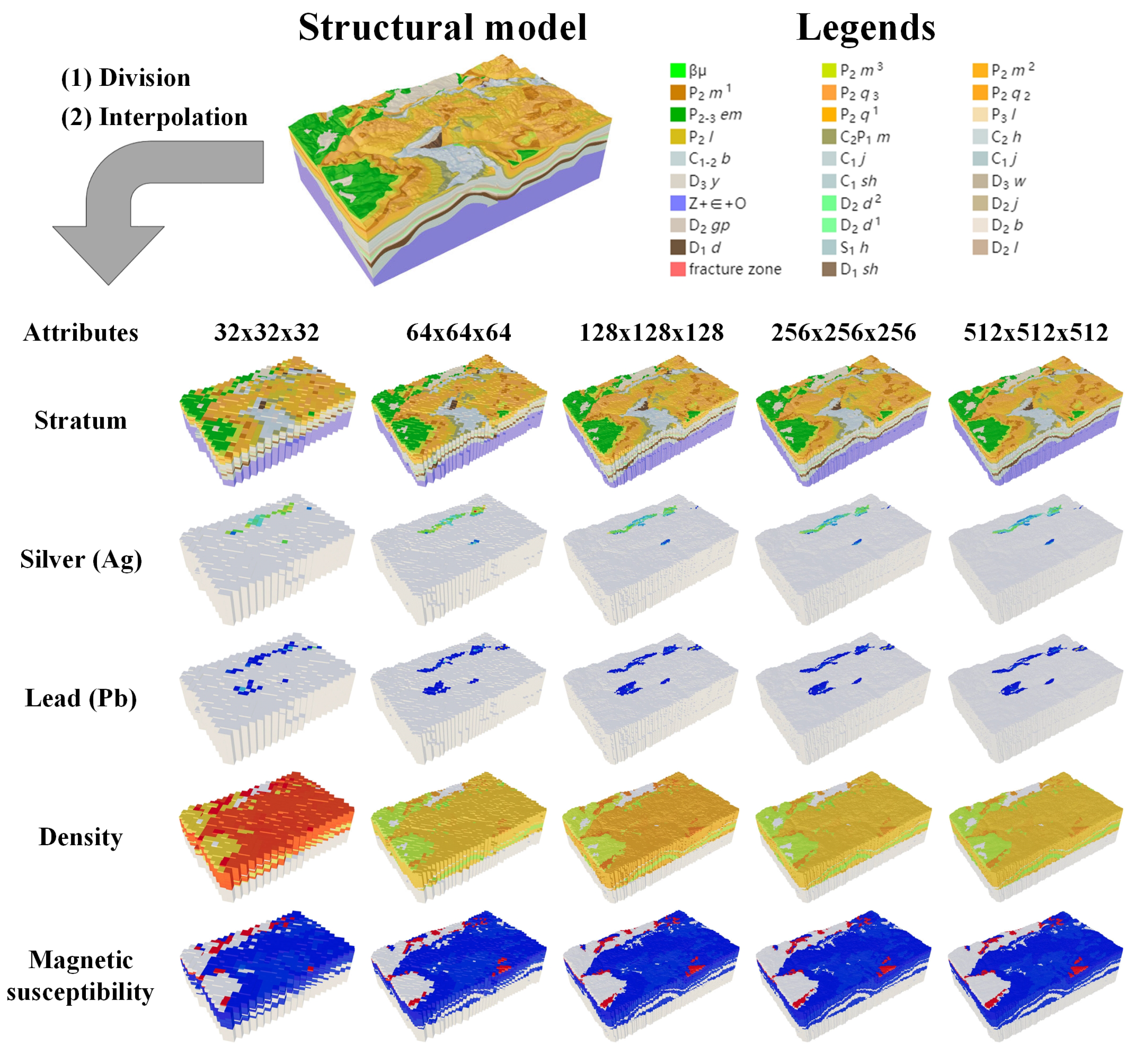
Data description. The experiments use a 1:250,000 3D geological model from the southwestern region of Guizhou Province, constructed from real geological survey data and regional geological interpretations. The model is voxelized and attribute values are interpolated to produce multiscale block datasets at five resolutions, as illustrated in Figure 9.

Table 1. Specifications of the 3D geological block datasets at five resolutions. Valid ratio (%) is the percentage of blocks with a true validity flag in the UDS at each resolution.

Datasets	Num of Blocks	Valid Blocks	Valid Ratio (%)
D32	32 × 32 × 32	16,406	50.06
D64	64 × 64 × 64	126,067	48.09
D128	128 × 128 × 128	983,021	46.87
D256	256 × 256 × 256	7,743,278	46.15
D512	512 × 512 × 512	61,452,258	45.79

reports the block counts and valid ratios at each resolution. The valid ratio at each resolution is defined as the percentage of blocks whose validity flag is true (i.e., blocks that contain geological information within the model extent) relative to the total number of blocks at that resolution. In the available dataset, only a limited number of geological attributes (such as lithology and a few physical properties) are consistently observed across all scales, and the number of tested resolution levels is constrained by the original survey design. As a result, the experiments reflect a realistic but still moderately sized industrial scenario. To enable a fair comparison and reliable assessment of efficiency, accuracy, and resource usage, the x, y, and z axes are partitioned uniformly so that data are evenly distributed across space.

Experimental environment. All experiments were conducted on a workstation equipped with an Intel^® Core™ i7-9700 CPU at 3.00 GHz with 8 cores, 64 GB RAM, and an NVIDIA Quadro P620 GPU, running Windows 10. The implementation is in Java with JDK 1.8.

Performance evaluation. The experiment consists of a benchmark experiment that measures the effect of attribute count, block size, and $L_{max}$ on the efficiency of WH-MSDM relative to VDB, Geohash, and Octree, followed by a comparative experiment on a very large dataset. The worst-performing baseline in the benchmark is omitted from the comparative experiment, which uses a dataset containing hundreds of millions of points. Integration efficiency is measured by time and storage footprint, while access efficiency is measured by query time and disk I/O. The benchmark issues 1000 random queries, and the comparative experiment issues 100 due to the large dataset scale. Query performance is reported as the average time and I/O counts per query after sorting each result set.

To estimate disk I/O under a cache-friendly setting, we assume sufficient memory to keep loaded disk blocks resident throughout execution and set the memory page size to 4 KB. During a query, we maintain an empty set S of disk block identifiers. For each index access at file position P, the block number b is computed as $[P/B]$ with block size B = 4096 bytes. If $b\in S$, no additional I/O is counted; otherwise, one I/O operation is recorded and b is inserted into S. The total I/O operations for the query are then ${IO}_{count}=\left|S\right|$.

3.2. Benchmark Experiments

We evaluate the effects of attribute count (AC), data size (DS), and maximum scale level ($L_{max}$) on WH-MSDM using a controlled variable design, keeping the query workload fixed for fairness and accuracy. The benchmark configurations are summarized in

Table 2. Benchmark settings for attribute count, data size, and maximum scale level.

Factors	Datasets	Attributes	Blocks	${\mathit{L}}_{\mathit{max}}$
AC	D32–128	4	2,392,064	3
	D32–128	5	2,392,064	3
DS	D32–64	5	294,912	2
	D64–128	5	2,359,296	2
$L_{max}$	D64–128	5	2,359,296	2
	D32–128	5	2,392,064	3

.

3.2.1. Effect of Attribute Counts

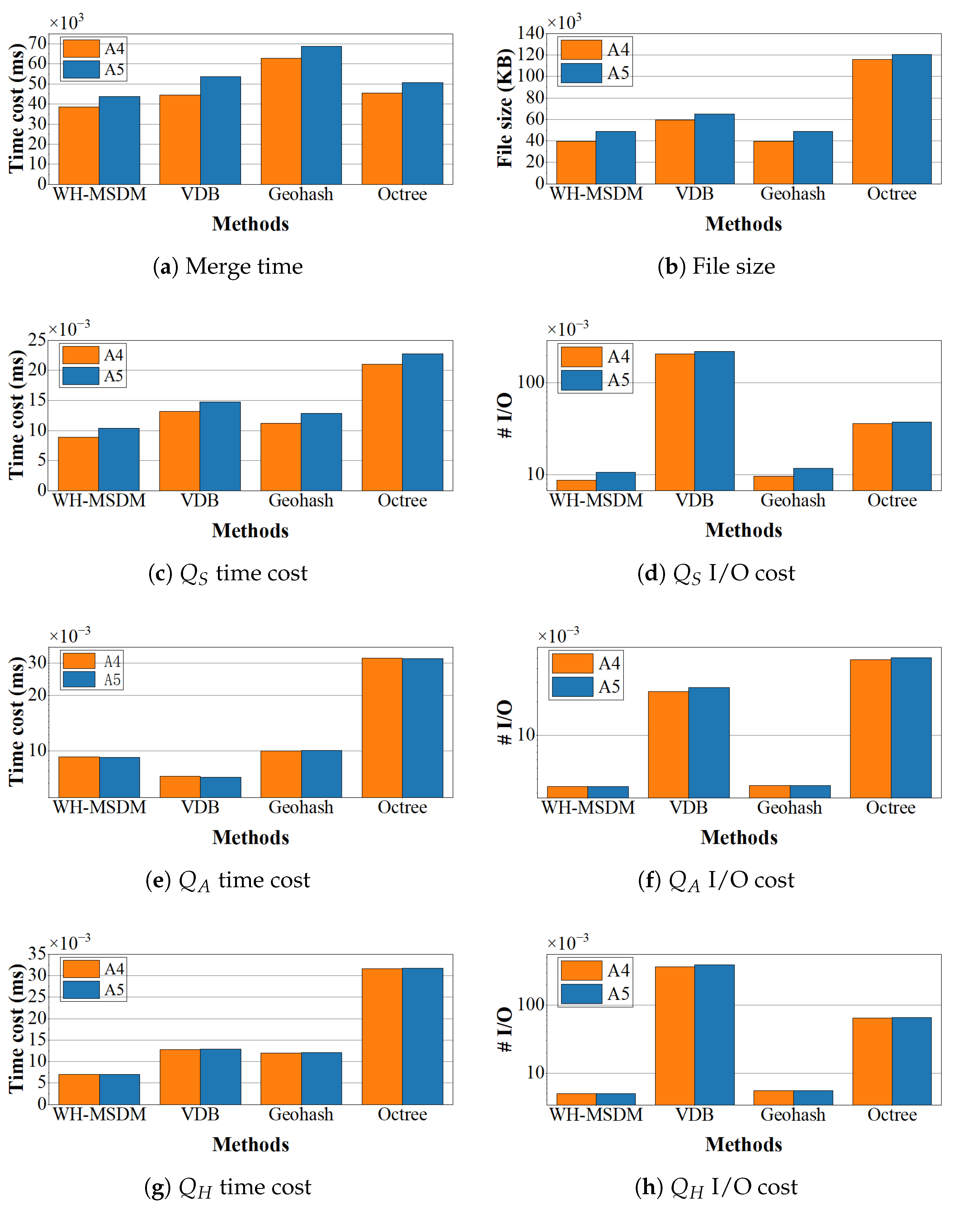
We compare $AC=4$ and $AC=5$ on the D32–128 dataset at level 3 (2,392,064 million blocks). Figure 10 presents organization time, storage footprint, and query performance across the four methods, and

Table 3. Effect of attribute counts on cross-scale queries.

Type	Algorithms	Time Cost (ms)		I/O
		A4	A5	A4	A5
$Q_{CP}$	WH-MSDM	0.14	0.15	5.00	6.00
	VDB	30.27	30.12	19.34	19.44
	GeoHash	0.07	0.07	5.00	6.00
	Octree	1280.71	1278.37	14,795.31	15,360.27
$Q_{CC}$	WH-MSDM	0.02	0.03	0.67	0.80
	VDB	3.98	3.98	2.58	2.58
	GeoHash	0.02	0.02	0.66	0.80
	Octree	21.70	21.88	1388.58	1421.45

summarizes cross-scale results.

Increasing attributes from 4 to 5 raises time and space costs for all methods. VDB shows the largest time increase (20.21%), while Geohash shows the smallest (9.63%). Storage grows by 23.53% for WH-MSDM and Geohash, and by 3.80% for Octree. For spatial queries (Figure 10c,d), WH-MSDM’s time and I/O rise by 17.01% and 22.58%, both lower than the competitors. For attribute queries (Figure 10e,f), WH-MSDM uniquely reduces time (0.76%) with stable I/O, indicating a favorable layout for attribute access. For hybrid queries (Figure 10g,h), WH-MSDM’s time increases by only 0.71% with no I/O change, suggesting strong robustness. By contrast, VDB and Octree exhibit higher I/O growth in spatial queries (6.95% and 3.83%), which can degrade disk I/O performance. These patterns are consistent with the cross-scale results in Table 3.

3.2.2. Effect of Data Size

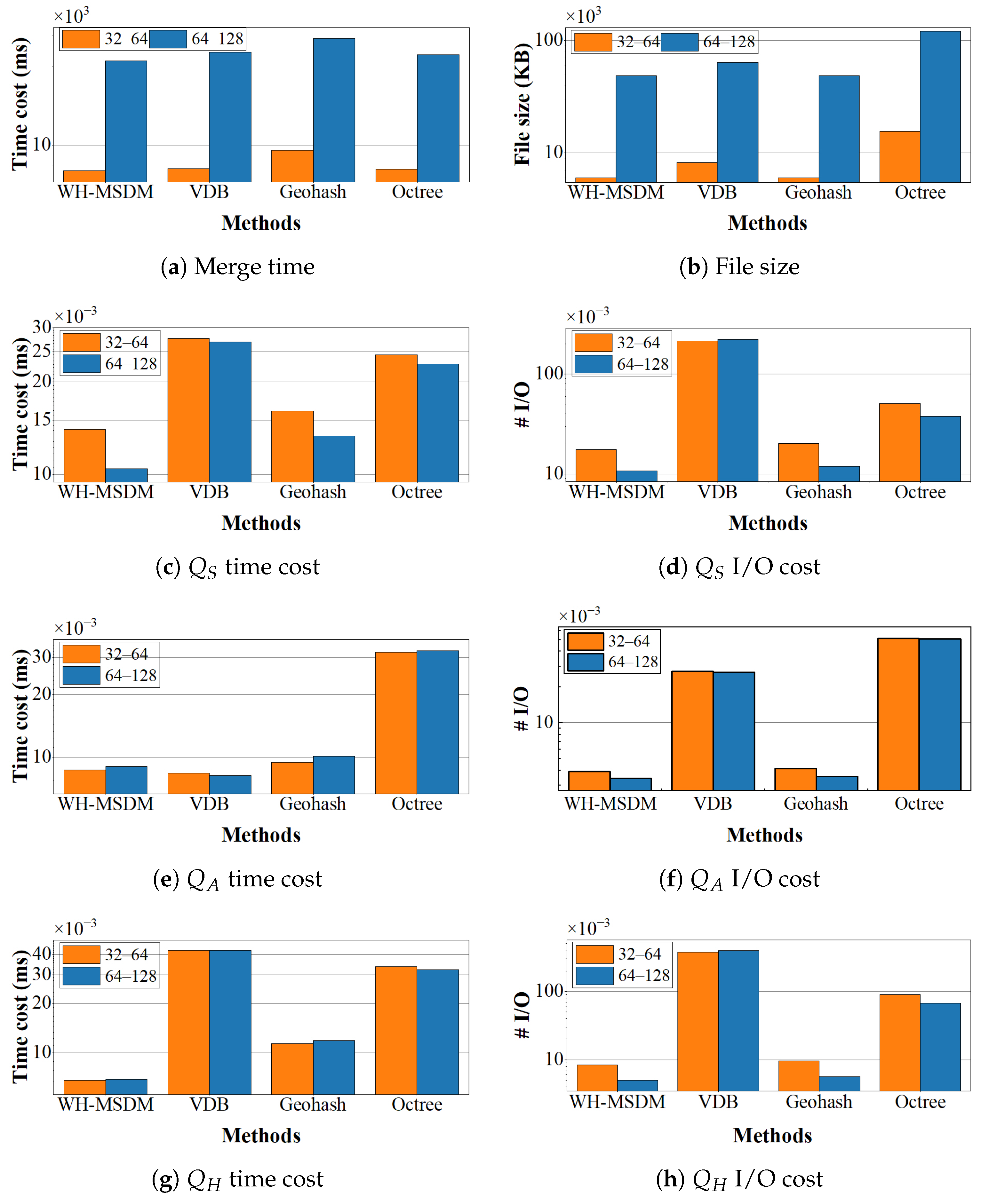
We next study data size by comparing D32–64 (294,912 blocks) and D64–128 (235,929,296 blocks), an eightfold increase with five attributes and $L_{max}=2$. Figure 11 presents organization and query metrics, and

Table 4. Effect of data size on cross-scale queries.

Type	Algorithms	Time Cost (ms)		I/O
		32–64	64–128	32–64	64–128
$Q_{CP}$	WH-MSDM	0.08	0.07	6.00	6.00
	VDB	26.35	187.57	19.25	123.23
	GeoHash	0.07	0.07	6.00	6.00
	Octree	320.55	2382.78	2056.81	14,766.12
$Q_{CC}$	WH-MSDM	0.02	0.02	0.80	0.77
	VDB	3.49	25.26	2.50	17.19
	GeoHash	0.02	0.02	0.80	0.77
	Octree	6.08	44.39	262.70	2059.59

reports cross-scale performance.

As size grows from 32–64 to 64–128, the methods diverge. For organization (Figure 11a,b), WH-MSDM increases by roughly 6 times in time and 7 times in space, while remaining stable. VDB rises by 6.8 times in time and 7.7 times in space, and Octree by 6.5 times and 6.8 times, respectively.

In spatial queries (Figure 11c,d), WH-MSDM’s time grows by 26% and I/O by 3%, whereas VDB increases by 6.8 times and 7.2 times. In attribute queries (Figure 11e,f), WH-MSDM reduces I/O by 13%, while VDB and Octree increase by 98%. During hybrid queries (Figure 11g,h), WH-MSDM decreases I/O by 40%, whereas VDB rises by 4.9%. Overall, data size has a stronger adverse effect on VDB and Octree, particularly in terms of I/O, while WH-MSDM maintains better stability and scalability. Table 4 further shows that WH-MSDM and Geohash remain stable in cross-scale queries, both relying on encoding before location lookup, whereas VDB and Octree incur roughly eightfold increases in time and I/O due to traversal along parent–child links.

3.2.3. Effect of $L_{max}$

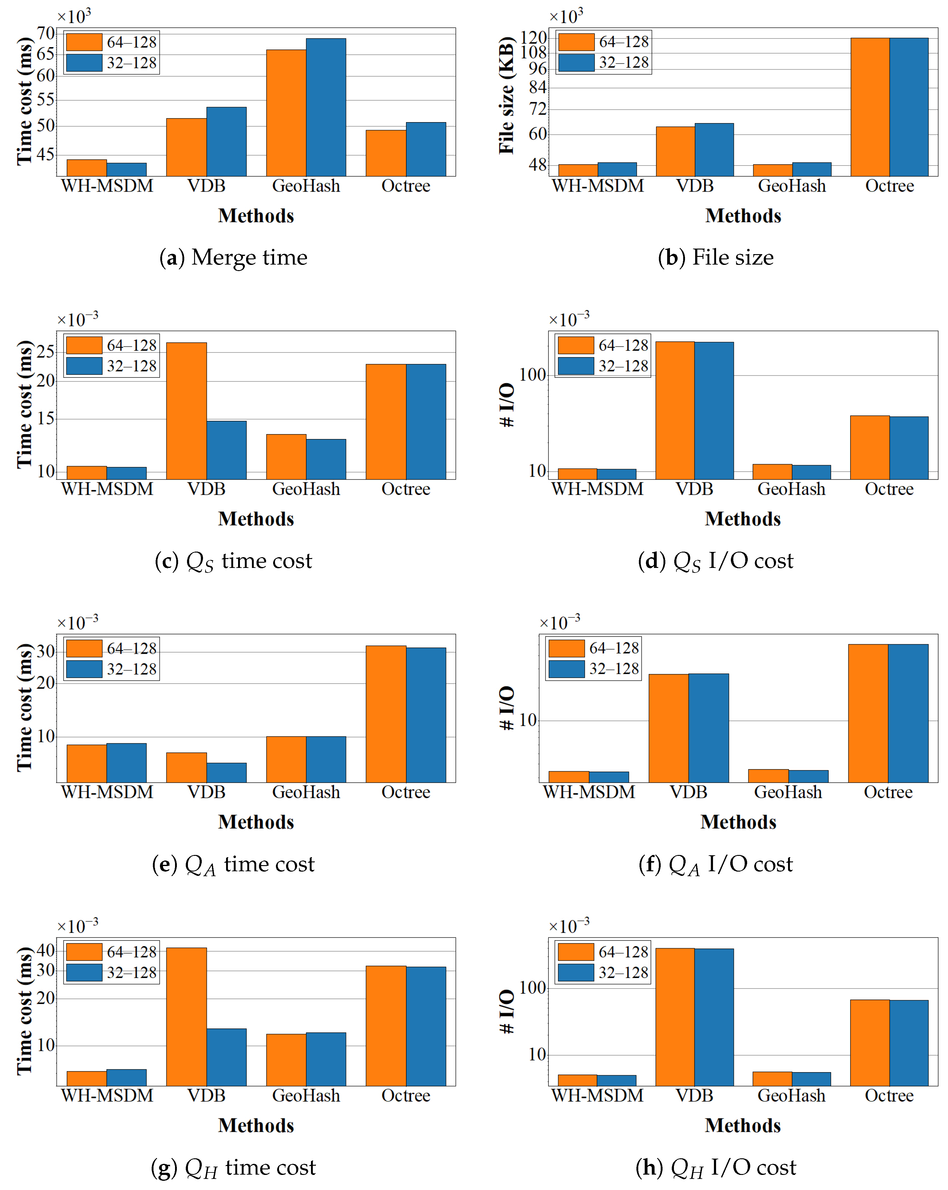
Finally, we examine the effect of the maximum scale level by comparing D64–128 (2,359,296 blocks, $L_{max}=2$) and D32–128 (2,392,064 blocks, $L_{max}=3$). The block difference is 32,768 blocks, corresponding to a 1.37% discrepancy that does not affect conclusions.

For organization (Figure 12a,b), WH-MSDM on D64–128 reduces time by 14.03% and space by 23.87% relative to VDB. On D32–128, the reductions are 18.47% and 24.78%. For spatial queries (Figure 12c,d), WH-MSDM on D64–128 lowers time by 61.32% and I/O by 95.18% versus VDB. On D32–128, it reduces time by 29.66% and I/O by 95.18%. For attribute queries (Figure 12e,f), WH-MSDM’s time on D64–128 is 10.66% higher than VDB but I/O is 87.21% lower. On D32–128, time is 28.36% higher and I/O is 87.37% lower. For hybrid queries (Figure 12g,h), WH-MSDM on D64–128 cuts time by 83.68% and I/O by 98.73%. On D32–128, it reduces time by 45.27% and I/O by 98.73%. As $L_{max}$ increases, WH-MSDM remains stable in both time and space, whereas VDB and Geohash fluctuate. When $L_{max}$ rises from 2 to 3, VDB’s time and space increase by 4.18% and 2.68%, while Geohash increases by 4.18% and 1.37%.

Table 5. Effect of $L_{max}$ on cross-scale queries.

Type	Algorithms	Time Cost (ms)		I/O
		64–128	32–128	64–128	32–128
$Q_{CP}$	WH-MSDM	0.07	0.15	6.00	6.00
	VDB	187.57	30.12	123.23	19.44
	GeoHash	0.07	0.07	6.00	6.00
	Octree	2382.78	1278.37	14,766.12	15,360.27
$Q_{CC}$	WH-MSDM	0.02	0.03	0.77	0.80
	VDB	25.26	3.98	17.19	2.58
	GeoHash	0.02	0.02	0.77	0.80
	Octree	44.39	21.88	2059.56	1421.45

shows that WH-MSDM and Octree improve in cross-scale queries, while VDB declines due to its traversal-based mechanism. Although Octree benefits from deeper hierarchies, its absolute speed remains limited. VDB’s degradation is driven by block-size effect at level 0, and Geohash, while stable, suffers from lower encoding and decoding efficiency, which contains overall performance.

3.3. Comparison with Other Methods

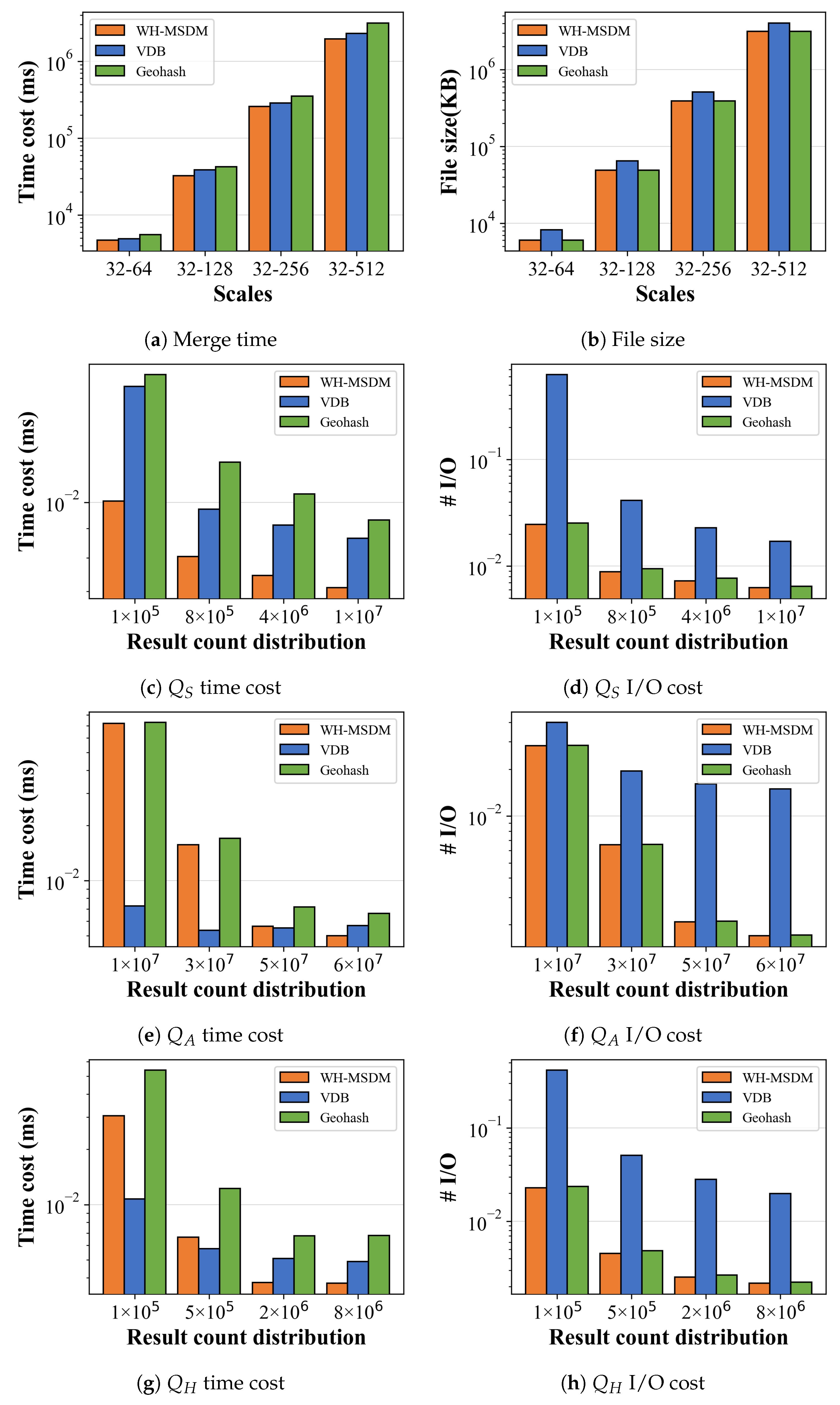
Given the clearly inferior organization and access efficiency of Octree in the benchmark experiments, we exclude it from the large-scale comparison to focus on the more competitive baselines and to reduce overall runtime. This section therefore compares the data organization and access efficiency of WH-MSDM against VDB and Geohash using a dataset containing more than 100 million blocks. As summarized in

Table 6. Comparison in data organization efficiency.

Metrics	Algorithms	32–64	32–128	32–256	32–512
Merge time (ms)	WH-MSDM	6305	40,176	316,716	1,952,573
	VDB	6572	47,878	345,504	2,297,068
	Geohash	6673	68,871	561,118	3,150,473
File size (KB)	WH-MSDM	6049	49,057	393,121	3,145,633
	VDB	8210	65,213	512,768	4,058,911
	Geohash	6049	49,057	393,121	3,145,633

, WH-MSDM reduces processing time by 10.1% relative to VDB and by 25.9% relative to Geohash, while using 32.0% less storage than VDB and matching the storage efficiency of Geohash.

Figure 13a,b compare organization time and file size. For smaller datasets, VDB exhibits organization times comparable to those of WH-MSDM, but its time cost increases significantly as the data size grows, primarily due to more complex partitioning and retrieval structures. Geohash consistently shows higher organization time yet nearly identical storage usage to WH-MSDM, indicating that it is storage-efficient but computationally more expensive. The additional overhead comes from repeated spatial bisection, extended encoding operations, recursive traversal, and boundary effects at grid edges.

Figure 13c,d show that WH-MSDM clearly outperforms VDB and Geohash in spatial queries. For the largest dataset, WH-MSDM reduces spatial query time by 24.9% relative to VDB and by 32.1% relative to Geohash, while lowering I/O counts by 93.4% and 4.2%, respectively. These gains stem from the compact block layout and W-Hilbert encoding, which favor sequential access and minimize redundant disk reads. Although Geohash achieves I/O counts similar to WH-MSDM, its more scattered spatial distribution leads to higher CPU overhead, and VDB’s non-contiguous block accesses become increasingly costly in both time and I/O as the dataset grows.

Figure 13e,f report attribute query performance. WH-MSDM improves over Geohash by 5.0% in time. VDB initially achieves lower time costs on small datasets, but as data grows to $6\times {10}^7$ points, WH-MSDM becomes 10.6% faster than VDB. In terms of I/O, WH-MSDM reduces operations by 56.9% compared with VDB and by 0.9% compared with Geohash, reflecting a more favorable mapping from attribute queries to disk blocks.

Hybrid query results in Figure 13g,h further highlight WH-MSDM’s advantages when spatial and attribute conditions must be combined. For large-scale data, WH-MSDM decreases hybrid query time by 24.8% relative to VDB and by 44.1% relative to Geohash, while reducing I/O by 93.8% and 3.8%, respectively. All methods benefit from spatial locality and caching as the result sets grow, which leads to an overall reduction in time and I/O, but WH-MSDM retains a clear lead across the tested scales.

Table 7. Comparison in cross-scale query performance.

Algorithms	${\mathit{Q}}_{\mathit{CP}}$		${\mathit{Q}}_{\mathit{CC}}$
	Time Cost (ms)	I/O	Time Cost (ms)	I/O
WH-MSDM	0.15	4.96	0.07	2.38
VDB	39.47	22.83	40.94	8.78
GeoHash	0.15	4.96	0.07	2.38

summarizes cross-scale query performance. WH-MSDM achieves the best efficiency for both parent queries ($Q_{CP}$) and child queries ($Q_{CC}$), primarily due to its explicit use of spatial clustering and Hilbert-based indexing. VDB mitigates the cost of cross-scale traversal by reducing the number of child nodes visited, yet remains significantly slower and more I/O-intensive. Geohash exhibits behavior very close to WH-MSDM in this setting, since both methods rely on encoding-based location lookup, though Geohash’s encoding and decoding overhead still limit its overall performance.

Overall, the comparative experiments show that WH-MSDM substantially improves both organization and querying of multiscale three-dimensional geological data, while maintaining stable time and space efficiency as the number of attributes and the data volume increase. In contrast, methods such as VDB and Octree incur higher I/O costs and larger time overheads due to more complex traversal patterns and indexing structures. Under large-scale conditions, WH-MSDM exhibits only modest performance degradation and sustains high efficiency across different maximum scale levels. In contrast, VDB becomes increasingly sensitive to block size and hierarchy depth. The combination of a compact global structure and efficient disk access enables WH-MSDM to deliver consistently strong performance for spatial, attribute, hybrid, and cross-scale queries.

4. Conclusions

This paper proposed WH-MSDM to address the management of geological data with uneven spatial distribution, multidimensional attributes, and multiscale structure. By combining a unified data structure (UDS), a bidirectional mapping model (BMM), and specialized query algorithms, WH-MSDM achieves more efficient and scalable data organization and querying than VDB, Geohash, and Octree. The UDS allows WH-MSDM to organize blocks from all resolutions within a single global framework, thereby accommodating highly non-uniform spatial distributions without duplicating data. In terms of data organization, WH-MSDM reduces organization time by 10.1% compared to VDB and 25.9% compared to Geohash while saving 32.0% of storage space relative to VDB.

On the query side, WH-MSDM provides dedicated procedures for spatial, attribute, hybrid, and cross-scale queries, which together support flexible access to multiscale and multidimensional geological attributes. Benchmark experiments consistently show lower query times and I/O costs compared to the baseline. For spatial queries, WH-MSDM is 24.9% faster than VDB and 32.1% faster than Geohash, while substantially reducing I/O overhead. As data size, attribute count, and maximum scale level $L_{max}$ increase, WH-MSDM maintains stable performance, whereas VDB and Octree exhibit clear degradation. By exploiting the BMM for efficient cross-scale mapping, the framework quickly and accurately retrieves parent and child blocks, thereby supporting seamless integration across levels of detail in multiscale analysis. The main contributions of this work can be summarized as follows: (1) a W-Hilbert-based unified data structure that assigns contiguous codes to blocks at all resolutions, enabling single-pass retrieval without redundant storage. (2) A bidirectional mapping model that dynamically links three-dimensional geological block coordinates to multiscale storage positions, supporting unified hierarchical indexing and efficient joint querying of geometric structure and multiscale attributes. (3) A suite of query algorithms for spatial, attribute, hybrid, and cross-scale access that improves the flexibility, precision, and efficiency of block data storage and retrieval in complex geological settings.

WH-MSDM is well-suited to practical multiscale applications such as regional geological surveys and mineral exploration, where reducing the time and computational resources required for data organization and querying directly improves analytical efficiency and supports resource management and environmental assessment. At the same time, WH-MSDM is complementary to recent multiscale geospatial grid management frameworks [32], which focus on grid design and indexing strategies at global scales. Despite the above advantages, WH-MSDM has several limitations and applicability conditions that should be noted. First, the current experiments are conducted on a real 1:250,000 3D geological model from southwestern Guizhou Province, but the available attribute set is still relatively modest and the number of tested resolution levels is limited. In real industrial deployments, such as large-scale mining or reservoir models, the attribute dimensionality and the range of scales may be substantially higher, which could increase index size and cache pressure. Second, the method assumes that the valid-block ratio is not extremely low. When the proportion of valid blocks becomes very small, storing identifiers for invalid blocks to maintain global spatial coherence can introduce additional overhead, and sparse representations such as VDB may become more favorable in terms of memory. Third, WH-MSDM is currently designed for grids that are locally regular in three dimensions. Highly anisotropic grids or strongly irregular stratigraphic geometries may require a more sophisticated coupling between the geological modeling step and the W-Hilbert-based indexing to avoid inefficiencies. Finally, although our implementation is CPU-based and demonstrates clear performance benefits, mapping the bidirectional mapping model and query operators efficiently to GPUs or other parallel architectures requires careful design of data layouts and memory access patterns, which we leave as future work.

References

1. Liu, H.; Xia, S.; Fan, C.; Zhang, C. 3D Geo-Modeling Framework for Multisource Heterogeneous Data Fusion Based on Multimodal Deep Learning and Multipoint Statistics: A case study in South China Sea. EGUsphere 2024, 2024, 1–44. [Google Scholar] [CrossRef]
2. Guo, H.; Goodchild, M.F.; Annoni, A. Manual of Digital Earth; Springer Nature: Berlin/Heidelberg, Germany, 2020. [Google Scholar]
3. Annoni, A.; Nativi, S.; Çöltekin, A.; Desha, C.; Eremchenko, E.; Gevaert, C.M.; Giuliani, G.; Chen, M.; Perez-Mora, L.; Strobl, J.; et al. Digital earth: Yesterday, today, and tomorrow. Int. J. Digit. Earth 2023, 16, 1022–1072. [Google Scholar] [CrossRef]
4. White, G.; Zink, A.; Codecá, L.; Clarke, S. A digital twin smart city for citizen feedback. Cities 2021, 110, 103064. [Google Scholar] [CrossRef]
5. Pan, D.; Xu, Z.; Lu, X.; Zhou, L.; Li, H. 3D scene and geological modeling using integrated multi-source spatial data: Methodology, challenges, and suggestions. Tunn. Undergr. Space Technol. 2020, 100, 103393. [Google Scholar] [CrossRef]
6. Li, F.; Gao, C.; Liu, Y.; Huang, K.; Pan, M.; Chen, X.; Yuan, Y. Integrated multi-scale reservoir data representation and indexing for reservoir data management and characterization. Comput. Geosci. 2020, 138, 104433. [Google Scholar] [CrossRef]
7. Islam, M.A.; Yunsi, M.; Qadri, S.T.; Shalaby, M.R.; Haque, A.E. Three-dimensional structural and petrophysical modeling for reservoir characterization of the Mangahewa formation, Pohokura Gas-Condensate Field, Taranaki Basin, New Zealand. Nat. Resour. Res. 2021, 30, 371–394. [Google Scholar] [CrossRef]
8. Yang, H.; Xu, X. Structure monitoring and deformation analysis of tunnel structure. Compos. Struct. 2021, 276, 114565. [Google Scholar] [CrossRef]
9. Gong, J.; Bao, T.; Zhu, Z.; Yu, H.; Li, Y. BIM-based framework of automatic tunnel segment assembly and deviation control. Undergr. Space 2024, 16, 59–78. [Google Scholar] [CrossRef]
10. Khan, M.S.; Kim, I.S.; Seo, J. A boundary and voxel-based 3D geological data management system leveraging BIM and GIS. Int. J. Appl. Earth Obs. Geoinf. 2023, 118, 103277. [Google Scholar] [CrossRef]
11. Niu, L.; Wang, Z.; Lin, Z.; Zhang, Y.; Yan, Y.; He, Z. Voxel-Based Navigation: A Systematic Review of Techniques, Applications, and Challenges. ISPRS Int. J. Geo-Inf. 2024, 13, 461. [Google Scholar] [CrossRef]
12. Mariethoz, G.; Caers, J. Multiple-Point Geostatistics: Stochastic Modeling with Training Images; John Wiley & Sons: Hoboken, NJ, USA, 2014. [Google Scholar]
13. Liu, F.; Yang, T.; Deng, W.; Zhou, J.; Li, J. Geostatistics-block-based characterization of heterogeneous rock mass and its application on ultimate pit limit optimization: A case study. Bull. Eng. Geol. Environ. 2021, 80, 1683–1700. [Google Scholar] [CrossRef]
14. Han, B.; Qu, T.; Tong, X.; Jiang, J.; Zlatanova, S.; Wang, H.; Cheng, C. Grid-optimized UAV indoor path planning algorithms in a complex environment. Int. J. Appl. Earth Obs. Geoinf. 2022, 111, 102857. [Google Scholar] [CrossRef]
15. Radwan, A.A.; Abdelwahhab, M.A.; Nabawy, B.S.; Mahfouz, K.H.; Ahmed, M.S. Facies analysis-constrained geophysical 3D-static reservoir modeling of Cenomanian units in the Aghar Oilfield (Western Desert, Egypt): Insights into paleoenvironment and petroleum geology of fluviomarine systems. Mar. Pet. Geol. 2022, 136, 105436. [Google Scholar] [CrossRef]
16. Cui, Z.; Chen, Q.; Liu, G. A two-stage downscaling hydrological modeling approach via convolutional conditional neural process and geostatistical bias correction. J. Hydrol. 2023, 620, 129498. [Google Scholar] [CrossRef]
17. Fan, W.; Liu, G.; Chen, Q.; Cui, Z.; Fang, H.; Chen, G.; Wu, X. Automatic reconstruction of geological reservoir models based on conditioning data constraints and BicycleGAN. Geoenergy Sci. Eng. 2024, 234, 212690. [Google Scholar] [CrossRef]
18. Li, Y.; Bai, M.; Guan, Q.; Ming, Z.; Liang, X.; Liu, G.; Gao, J. CSD-R k NN: Reverse k nearest neighbors queries with conic section discriminances. Int. J. Geogr. Inf. Sci. 2023, 37, 2175–2204. [Google Scholar] [CrossRef]
19. Wang, Y.; Lv, H.; Ma, Y. Geological tetrahedral model-oriented hybrid spatial indexing structure based on Octree and 3D R*-tree. Arab. J. Geosci. 2020, 13, 728. [Google Scholar] [CrossRef]
20. Li, B.; Wang, J.; Zhang, Y.; Sun, Y. Innovative Adaptive Multiscale 3D Simulation Platform for the Yellow River Using Sphere Geodesic Octree Grid Techniques. Water 2024, 16, 1791. [Google Scholar] [CrossRef]
21. Zhao, L.; Li, G.; Yao, X.; Ma, Y.; Cao, Q. An optimized hexagonal quadtree encoding and operation scheme for icosahedral hexagonal discrete global grid systems. Int. J. Digit. Earth 2022, 15, 975–1000. [Google Scholar] [CrossRef]
22. Museth, K. VDB: High-resolution sparse volumes with dynamic topology. ACM Trans. Graph. TOG 2013, 32, 1–22. [Google Scholar] [CrossRef]
23. Aleksandrov, M.; Zlatanova, S.; Heslop, D.J. Voxelisation algorithms and data structures: A review. Sensors 2021, 21, 8241. [Google Scholar] [CrossRef] [PubMed]
24. Yan, H.; Liu, C.; Ma, C.; Mei, X. Plenvdb: Memory efficient vdb-based radiance fields for fast training and rendering. In Proceedings of the IEEE/CVF Conference on Computer Vision and Pattern Recognition, Vancouver, BC, Canada, 17–24 June 2023; pp. 88–96. [Google Scholar]
25. Liu, Z.; Chen, L.; Yang, A.; Ma, M.; Cao, J. Hiindex: An efficient spatial index for rapid visualization of large-scale geographic vector data. ISPRS Int. J. Geo-Inf. 2021, 10, 647. [Google Scholar] [CrossRef]
26. Lei, Y.; Tong, X.; Qu, T.; Qiu, C.; Wang, D.; Sun, Y.; Tang, J. A scale-elastic discrete grid structure for voxel-based modeling and management of 3D data. Int. J. Appl. Earth Obs. Geoinf. 2022, 113, 103009. [Google Scholar] [CrossRef]
27. Rifai, M.; Johnsson, L. VxH: A Systematic Determination of Efficient Hierarchical Voxel Structures. ACM Trans. Spat. Algorithms Syst. 2023, 10, 1–34. [Google Scholar] [CrossRef]
28. Zhang, X.; Wang, L.; Zhou, Z.; Niu, Y. A chaos-based image encryption technique utilizing Hilbert curves and H-fractals. IEEE Access 2019, 7, 74734–74746. [Google Scholar] [CrossRef]
29. Li, M.; Wang, H.; Dai, H.; Li, M.; Chai, C.; Gu, R.; Chen, F.; Chen, Z.; Li, S.; Liu, Q.; et al. A survey of multi-dimensional indexes: Past and future trends. IEEE Trans. Knowl. Data Eng. 2024, 36, 3635–3655. [Google Scholar] [CrossRef]
30. Jia, L.; Chen, M.; Li, M.; You, J.; Ding, J. State view based efficient Hilbert encoding and decoding algorithms. J. Electron. Inf. Technol. 2020, 42, 1494–1501. [Google Scholar]
31. Lei, Y.; Tong, X.; Wang, D.; Qiu, C.; Li, H.; Zhang, Y. W-Hilbert: A W-shaped Hilbert curve and coding method for multiscale geospatial data index. Int. J. Appl. Earth Obs. Geoinf. 2023, 118, 103298. [Google Scholar] [CrossRef]
32. Su, Y.; Zhu, D.; Xiao, B.; Li, S.; Qu, T.; Zhai, W.; Cheng, C. Geospatial grid management: A comprehensive framework and systematic review of subdivision, encoding, indexing and storage. Int. J. Appl. Earth Obs. Geoinf. 2025, 144, 104860. [Google Scholar] [CrossRef]
Figure 1. W-Hilbert code distribution across scales in 3D ( L max = 2 ) [31]. It demonstrates how blocks at levels 0, 1, and 2 receive base codes and intra-level offsets to maintain spatial locality.
Applsci 15 13112 g001
Figure 2. Schematic of the unified data structure (UDS) in WH-MSDM, which depicts metadata, validity bitmask, and packed attributes.
Applsci 15 13112 g002
Figure 3. Workflow of the bidirectional mapping model (BMM) in WH-MSDM. It outlines encoding 3D coordinates into UDS and decoding back to spatial positions.
Applsci 15 13112 g003
Figure 4. Level determination and location mapping from W-Hilbert codes, which illustrates how counting trailing “1” bits in a W-Hilbert code yields its scale level, and how that code maps to a global storage index in UDS.
Applsci 15 13112 g004
Figure 5. Intra-group re-encoding example: after external offsets are applied, the original block number (630) is renumbered to the current group encoding (6) for zero-based local block queries.
Applsci 15 13112 g005
Figure 6. Left-sibling re-encoding: left siblings are collected, external offsets are applied, and blocks are renumbered from zero for range lookups.
Applsci 15 13112 g006
Figure 7. BMM deconstruction steps: external offset computation, intra-group re-encoding, and final spatial reconstruction.
Applsci 15 13112 g007
Figure 8. Cross-scale binary patterns. Parent and child codes differ only in the lowest D × ( L m a x L ) + 1 bits, which supports tight query bounds.
Applsci 15 13112 g008
Figure 9. 3D block layouts at five resolutions, from 32 3 to 512 3 grids, where the superscript ’3’ denotes the N × N × N grid size consistent with the 3D layout.
Applsci 15 13112 g009
Figure 10. Effect of attribute counts ( 4 5 ) on organization and access: (a) Organization time, (b) Storage footprint, (c) Spatial query time, (d) Spatial query I/O, (e) Attribute query time, (f) Attribute query I/O, (g) Hybrid query time, (h) Hybrid query I/O.
Applsci 15 13112 g010
Figure 11. Effect of data size ( 32 3 + 64 3 64 3 + 128 3 ) on organization and access: (a) Organization time, (b) Storage footprint, (c) Spatial query time, (d) Spatial query I/O, (e) Attribute query time, (f) Attribute query I/O, (g) Hybrid query time, (h) Hybrid query I/O.
Applsci 15 13112 g011
Figure 12. Effect of L m a x ( 2 3 ) on organization and access: (a) Organization time, (b) Storage space, (c) Spatial query time, (d) Spatial query I/O, (e) Attribute query time, (f) Attribute query I/O, (g) Hybrid query time, (h) Hybrid query I/O.
Applsci 15 13112 g012
Figure 13. Comparison of WH-MSDM and baseline methods in aggregate build, storage, and query performance. In all panels, the x-axis denotes the total number of blocks in the model. Panel (a) shows the merge time required to build the unified data structure, and panel (b) shows the resulting file size. Panels (c,e,g) show the average time cost per query for spatial queries ( Q S ), attribute queries ( Q A ), and hybrid queries ( Q H ), respectively. Panels (d,f,h) show the corresponding I/O operations per query. The legend distinguishes WH-MSDM from the baseline indexing methods.
Applsci 15 13112 g013