Article

Prediction of Soft Soil Settlement Based on Ensemble Smoother with Multiple Data Assimilation

1
Power China Huadong Engineering Co., Ltd., Hangzhou 310014, China
2
Zhejiang Engineering Research Center of Green Mine Technology and Intelligent Equipment, Hangzhou 310014, China
3
College of Civil Engineering, Zhejiang University of Technology, Hangzhou 310023, China
4
Zhejiang Key Laboratory of Green Construction and Intelligent Operation & Maintenance for Coastal Infrastructure (Zhejiang University of Technology), Hangzhou 310023, China
*
Author to whom correspondence should be addressed.
Appl. Sci. 2025, 15(24), 13074; https://doi.org/10.3390/app152413074
Submission received: 23 October 2025 / Revised: 5 December 2025 / Accepted: 10 December 2025 / Published: 11 December 2025

Abstract

The selection of soil parameters relies heavily on the engineering experience of practitioners and frequently results in settlement predictions that deviate from field monitoring, especially for soft soil foundations. This study proposes a settlement prediction method for soft soil based on the ensemble smoother with multiple data assimilation (ES-MDA), which makes use of monitoring data by updating the preliminarily selected soil parameters for improved settlement predictions. This study investigates the applicability of the ES-MDA for embankment settlement prediction. A real project on the northern coast of Zhejiang, China, is used to illustrate the implementation and practical feasibility of the ES-MDA method. After adaptive parameter updates using the ES-MDA algorithm, the uncertainty of the soil parameters is significantly reduced. Through iterative integration of observational data, the predicted mean settlement gradually approaches the measured values, while the 95% prediction interval becomes narrower, validating the effectiveness of the method. The data assimilation-based settlement prediction method is beneficial for risk management and the long-term maintenance of the embankment.

1. Introduction

Predicting the settlement of embankments constructed on soft soils is important for the design and construction planning of embankments, as well as for ensuring the safety and serviceability of the roadway [1,2]. Embankment settlement prediction is usually conducted by inputting soil parameters into analytical or numerical models [3,4,5]. The required soil parameters may be obtained from in situ tests, laboratory tests, or indirectly inferred from other measurable parameters through transformation models. However, engineering practice has shown that such predictions often diverge significantly from field monitoring results. This discrepancy can be attributed primarily to two factors, including the uncertainty in the selection of soil parameters and imperfections in the predictive models [6,7]. The uncertainty in soil parameter selection arises from several factors. Site investigations typically cover a limited number of locations, while soil properties exhibit spatial variability [8,9,10,11]. As a result, test samples may not be sufficiently representative of the entire site. Furthermore, the test results themselves are subject to uncertainty due to sampling and measurement errors. If soil parameters are derived indirectly through empirical correlations or transformation models, additional uncertainty is introduced through transformation errors [12,13]. Model-related uncertainties stem from simplifications inherent in both analytical and numerical approaches. These include idealizations in geometry, boundary conditions, and the construction process, which are often necessary to make the problem tractable but may compromise accuracy. Kelly et al. [14] summarized the outcomes of an embankment settlement prediction symposium and found that even when identical project information and test data were provided, different predictors produced markedly different settlement predictions. This variation is primarily attributed to subjective judgment in the selection of predictive models and in the interpretation of test results, the latter of which leads to differing estimates of the characteristic values of soil parameters.
With the rapid advancement of monitoring technologies, monitoring sensors are often installed during the construction and operation phases of embankments, providing multi-stage, multi-location, and multi-type monitoring data [15]. To utilize such data for improving settlement or deformation predictions, current research approaches can be broadly classified into data-driven machine learning methods [16,17,18,19,20] and inverse analysis methods [21,22,23,24]. Data-driven approaches typically do not consider the underlying physical mechanisms. Instead, they rely on large volumes of historical monitoring data to train and validate predictive models. As a result, these methods generally require a large amount of past settlement data and are inapplicable in the early stages of embankment construction when limited monitoring data is available. In contrast, inverse analysis methods incorporate physical models and use available monitoring data to back-calculate soil parameters, such as key parameters in constitutive models. As monitoring data accumulates over time, these soil parameter estimates and the corresponding settlement predictions can be continuously updated. Compared to machine learning approaches that typically require large volumes of historical data for model training, inverse analysis methods demand significantly less data. This is primarily because inverse analysis focuses on calibrating the parameters of a forward physical model using available measurements. With a physics-based model as the foundation, the method reduces dependency on data quantity while retaining strong extrapolation capabilities. In practical engineering applications, such as during the early stages of embankment construction, settlement progresses rapidly, and monitoring is conducted at high frequencies, potentially on a daily basis. As the settlement stabilizes, the monitoring frequency decreases, often to intervals of several days or even a week. In other words, the amount of data collected from embankment settlement monitoring is relatively limited compared to the data requirements for training machine learning models, making inverse analysis a more suitable approach in such contexts.
Among the inverse analysis approaches, probabilistic inverse analysis based on Bayes’ theorem has gained popularity for updating the distribution of poorly known parameters for better predictions. It provides a rational framework to incorporate different sources of information with quantified uncertainties, where the probability distributions of soil parameters are initially assumed according to existing knowledge (e.g., in situ and laboratory tests) and subsequently updated based on new observations. A popular probabilistic inverse analysis method in predicting settlement is the Bayesian method derived by Markov Chain Monte Carlo sampling (MCMC) [25,26,27,28]. MCMC provides rigorous sampling; however, it is computationally expensive due to the large number of forward model evaluations required, and this computational cost will further increase if the Bayesian updating needs to be performed repeatedly as new observation data become available.
Recently, ensemble-based data assimilation methods have been introduced to geotechnical engineering. The ensemble methods applied in geotechnical problems include the extended Kalman filter (EKF) and the ensemble Kalman filter (EnKF) [29,30,31,32,33,34,35]. For example, Hommels et al. [35] improved the settlement predictions by assimilating the sequentially observed settlements based on EnKF. EnKF is a Monte Carlo approximation of the standard Kalman filter (KF), as the mean and covariance matrix of the state (or target parameters) are directly evaluated by ensemble members. Hence, EnKF is easy to implement in the nonlinear and high-dimensional forward model. It is also computationally efficient as the required number of samples is significantly smaller than that of MCMC. However, the derivation of EnKF adopts the assumptions of linearization and Gaussian distributions of priors and measurement error. The update step in the EnKF is performed through a linear “shift” between the prior estimate and the observations, constituting a fundamentally linear update step. For nonlinear problems, the EnKF does not draw samples from the true posterior distribution but instead yields an approximation. When the discrepancy between predictions and measurements becomes large at a given time step, the EnKF may produce a significant overcorrection.
Another ensemble method that is closely related to EnKF but further reduces the computational cost is the ensemble Kalman smoother (ES). Unlike EnKF, which assimilates the sequential observations one by one, ES makes a single update using all past observations as a whole. Previous studies have shown that ES is inferior to EnKF in nonlinear problems [36,37]. This is because the sequential EnKF performs recursive and small updates over time, which can be regarded as multiple local linear approximations, while ES adopts a single linear update, resulting in deviations from the truth in the highly nonlinear forward model. Thus, Emerick and Reynolds [38] introduced an iterative procedure into ES to better preserve the original nonlinearity. This is achieved by recursion of the likelihood with inflated measurement errors, which means the standard ES using all past observations needs to be rerun several times and is thus called the ensemble smoother with multiple data assimilation (ES-MDA). The consolidation analysis and settlement prediction of soft ground improved with prefabricated vertical drains are inherently nonlinear problems. ES-MDA can convert the single large update required when incorporating monitoring data into multiple smaller updates, thereby preserving the original nonlinear behavior of the numerical model.
This study aims to enhance embankment settlement prediction by incorporating field monitoring data through the ensemble smoother with multiple data assimilation (ES-MDA). The contributions of this work are threefold. First, an ES-MDA-based probabilistic settlement prediction method is established for embankments with prefabricated vertical drains, in which the compression index and the equivalent vertical permeability of multiple soil layers are jointly updated using limited monitoring data. The posterior distributions of these parameters are characterized rather than calibrated as single best-fit values. Second, coupled consolidation analysis of PVD-improved soft ground is embedded into the ES-MDA procedure by introducing a long short-term memory surrogate model trained on finite element simulations, which reduces the computational cost of iterative updating and enables field-scale applications. Third, the effects of the amount and timing of monitoring data on prediction accuracy and uncertainty are evaluated using a real embankment. This study provides a data-informed pathway for improving settlement prediction and risk management in embankments constructed on soft ground.

2. Bayesian Updating Framework

Let x denote the soil parameters, and y denote the calculated system response. The forward model can then be written as y = (x). The measurement d of the system response y is available, with associated observation error. Our problem is to estimate and update the parameters x based on the available measurements d. This is an inverse problem and can be solved by Bayesian inference. The posterior distribution of the parameters p ( x | d ) can be written as
p ( x | d ) p ( d | x ) p ( x )
where p ( x ) is the prior distribution determined by the existing information of x, and p ( d | x ) refers to the likelihood function of measurements d given the forward model H ( x ) . Due to the nonlinear forward model in geotechnical problems, MCMC methods are usually used to derive the posterior distribution [39], which conduct rigorous sampling and are called the gold standard of Bayesian inference [40]. MCMC methods are capable of deriving complex posteriors involving any type of prior and likelihood, although the soil parameters and the observation errors are usually assumed to follow lognormal and normal distributions, respectively [28,41].
Soil settlement is a time-series problem, and the observations are obtained sequentially, as shown in Figure 1. As mentioned in the introduction, when performing MCMC-based Bayesian updating for soil settlement, it is more common to use all past observations as a whole (i.e., observations 1~nob) rather than to incorporate every individual observation as soon as it becomes available (the ith observation). EnKF assimilates observations one by one and makes an update once a new observation is obtained. In contrast, ES-MDA makes Nmda updates, and each update uses all historical data.
ES-MDA uses all available observations simultaneously. To alleviate the impacts of nonlinearity, ES-MDA performs a sequence of small linear updates by using a recursive form of the likelihood function:
p ( d | x ) = p ( d | x ) k = 1 N mda 1 / α k = k = 1 N mda p ( d | x ) 1 / α k
where k = 1 N mda 1 / α k = 1 , Nmda denotes the total number of iterations, and αk is the inflated coefficient for the covariance matrix of observation errors. The value of αk can be set as αk = Nmda. By substituting the recursive likelihood function into Equation (1), the posterior distribution is rewritten as
p ( x | d ) p ( x ) k = 1 N mda p ( d | H ( x k 1 ) ) 1 / α k
The cost function can be expressed as
J ( x k , i ) = 1 2 x k , i x k , i f P k 1 2 + 1 2 d + α k ε H ( x k , i ) ( α k R ) 1 2
where i represents the ith ensemble member, and k denotes the kth iteration. For each ensemble member, the observation vector d is perturbed by adding an inflated observation error α k ε , where ε ~ N 0 , R . This recursive form does not introduce any approximation, and ES-MDA and ES are equivalent in linear problems [38,42]. After some rearrangements, the update step in ES-MDA is written as
x k , i a = x k , i f + P k H T ( α k R + HP k H T ) 1 ( d + α k ε H x k , i f )
The implementation steps of ES-MDA are similar to those of EnKF, except that all the observations are used simultaneously in the update step in Equation (5) with inflated observation errors. The total number of iterations is determined by the prespecified value of Nmda instead of the number of observations.

3. Case Study

3.1. Project Overview

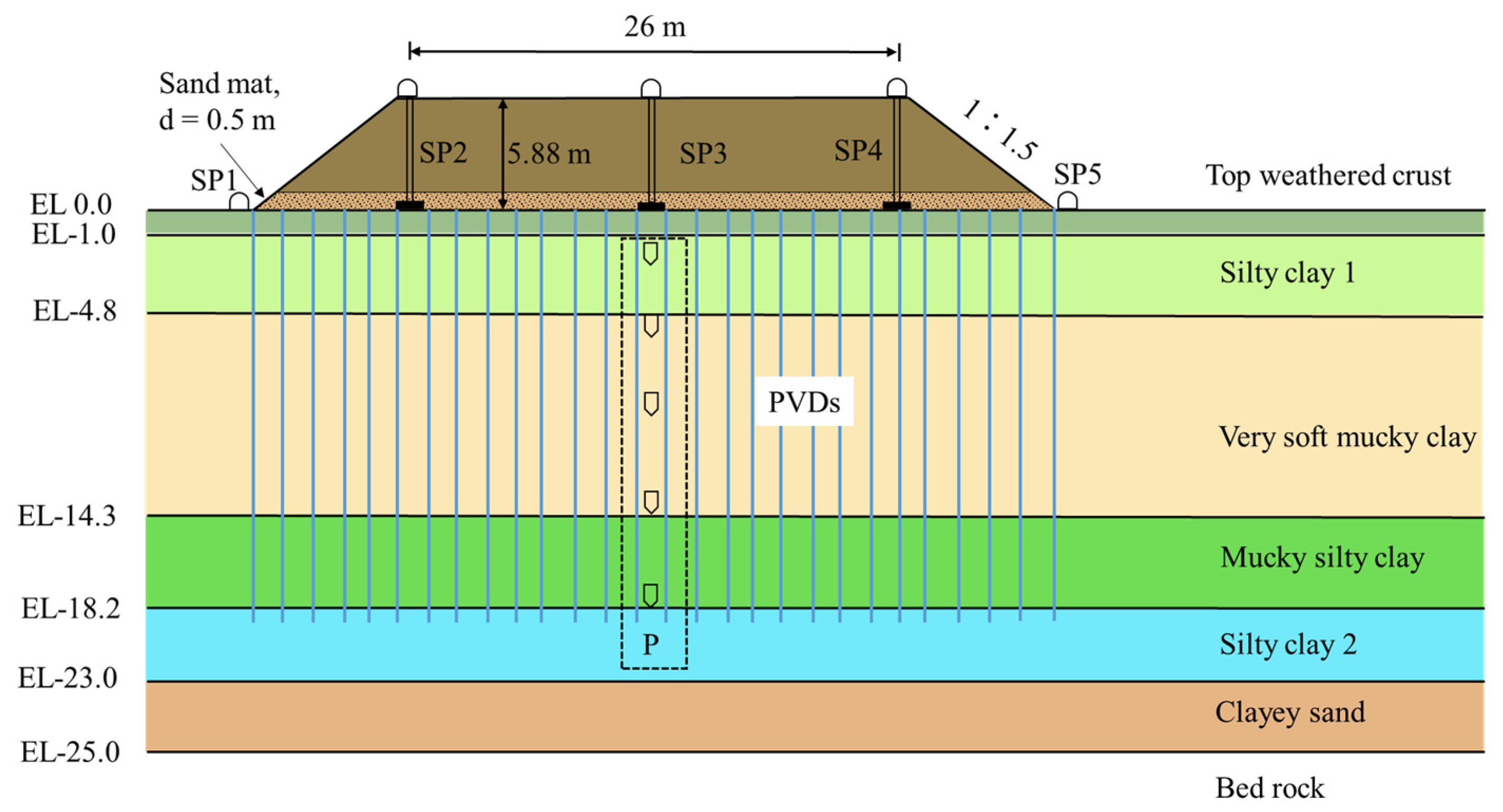
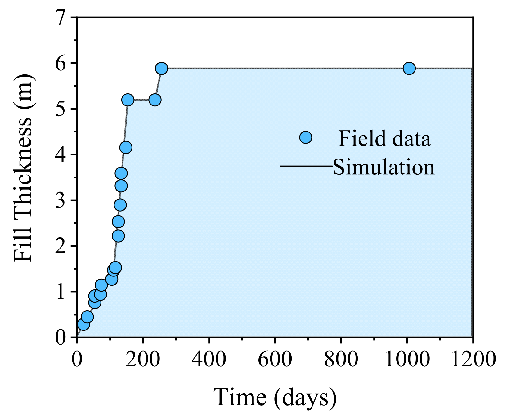
A real project is used to illustrate and evaluate the settlement prediction method based on ES-MDA. The project is located in Hangzhou, China. Based on the borehole and cone penetration test (CPT), the soil profile can be divided into six soil layers overlying the bedrock, composed of weathered rock. The specific layers include a 1 m thick top weathered crust (TC), a 3.8 m thick silty clay layer (SC1), a 9.5 m thick very soft mucky clay layer (MC), a 3.9 m thick mucky silty clay layer (MSC), a 4.8 m thick silty clay layer (SC2), and a 2 m thick clayey sand layer (CS). Above the ground surface, there is a 0.5 m thick sand cushion and a 5.38 m thick fill layer. Settlement plates (SPs) are installed at the center of the embankment surface, on both shoulders, and at the toes of the slopes on both sides. Piezometers (P) are placed at different depths along the centerline of the embankment, while inclinometers (Inclo) are positioned on both sides of the slopes and at the toe regions. The spacing (SL) of prefabricated vertical drains (PVDs) is 1.5 m, with a depth of 19 m. The problem geometry and embankment construction sequence are shown in Figure 2 and Figure 3, respectively.

3.2. Numerical Simulation

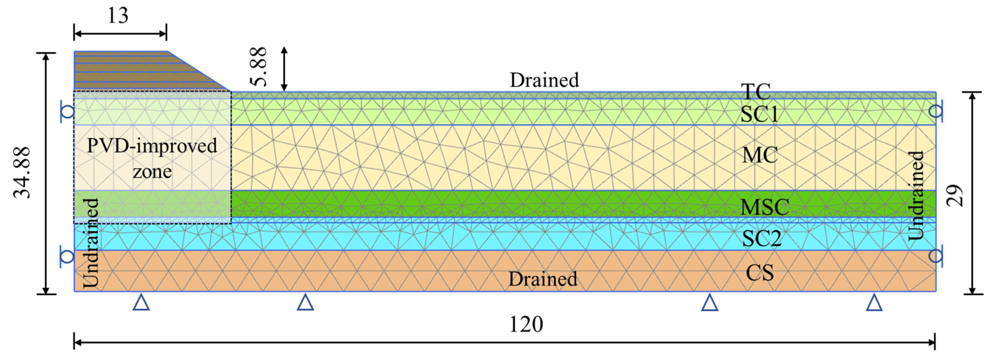
A finite element simulation is performed to model half of the embankment using PLAXIS 2D V20. The horizontal displacements are zero for the left and right boundaries, and the horizontal and vertical displacements are zero for the bottom boundary. The ground surface and bottom boundaries are permeable. The left and right boundaries are impermeable. The finite element mesh is generated using PLAXIS’s built-in fine mesh setting, and additional manual refinement is applied to the soft soil layers beneath the fill. A diagram of the finite element model is shown in Figure 4. The Modified Cam-clay (MCC) model is adopted to model the five clay layers, and the Mohr–Coulomb (MC) model is adopted for the fill and the clayey sand layer. Table 1 summarizes the soil parameters, which are either obtained directly from laboratory tests or indirectly transformed from other measured soil properties [43]. Specifically, the unit weight γ is calculated from the density test results, while the initial void ratio e0 is determined using the outcomes of the density, specific gravity, and water content tests. The compression index Cc and permeability coefficients (kh, kv) are obtained from specialized oedometer tests, with kh and kv measured from horizontally and vertically oriented soil specimens, respectively. The MCC parameter λ is transformed from the compression index using λ = Cc/2.3, and the parameter κ is set to 0.1λ [44]. The remaining parameters are adopted from the numerical analysis of Chai et al. [43].
To reflect the vertical drainage effect of natural subsoil as well as the radial drainage effect induced by the installation of PVDs, an equivalent vertical hydraulic conductivity kve is used in the finite element model, which simplifies the behavior of PVD-improved subsoil into a form analogous to that of unimproved subsoil. The equivalent vertical hydraulic conductivity kve is calculated as follows [43]:
k ve = 1 + 2.5 l 2 μ D e 2 k h k v k v
where kh and kv are the hydraulic conductivity in the horizontal and vertical directions, respectively; l is the drainage length; De represents the diameter of the unit cell, which is equal to 1.05SL; and the value of the PVD geometry factor μ can be expressed as
μ = ln n s + k h k s ln ( s ) 3 4 + π 2 l 2 k h 3 q w
where n = De/dw; the diameter of the vertical drain dw = (w + d)/2; w is the width of a band-shaped PVD; d is the thickness of the PVD; s = ds/dw, and ds represents the diameter of the smear zone; ks is the horizontal conductivity in the smear zone; and qw is the discharge capacity of the PVD in the field. The parameters related to the PVDs are summarized in Table 2.
The soil parameters to be updated are the compression index λ of the five soil layers under the fill layer and the equivalent vertical hydraulic conductivity kve of the four soil layers under the fill layer. This selection is made because the compression index λ directly reflects the soil compressibility and strongly affects the consolidation settlement [45], and the soil modulus is deemed to have high uncertainties [11]. The permeability parameter is also sensitive to consolidation calculation and is considered to have a higher degree of variation [46,47,48]. Considering that the total thickness of the SC2 layer is 4.8 m, while the installation depth of the PVDs is only 0.8 m, the drainage paths do not fully penetrate the layer. Therefore, the influence of the PVDs on the equivalent permeability coefficient of the SC2 layer is neglected. The prior distributions of λ and k are listed in Table 3, of which the mean values are set to the values estimated from the oedometer tests, with a coefficient of variation (COV) of 0.5 for λ and a COV of 1 for kve. The soil parameters are assumed to follow lognormal distributions so that they remain strictly positive throughout the updating process, given that the soil compression index and hydraulic conductivity cannot be zero or negative from a physical standpoint [31,49]. Settlement monitoring data are collected along the centerline at the base of the embankment. The monitoring time points 1 to 28 correspond to days 131, 148, 154, 155, 162, 173, 181, 196, 212, 228, 237, 257, 265, 281, 301, 314, 344, 381, 412, 461, 496, 537, 580, 629, 693, 782, 860, and 1013, respectively. The monitoring frequency is relatively high during the initial stage and is gradually reduced as the deformation rate stabilizes. The observation error of settlement is assumed to be white Gaussian noise with a standard deviation of 0.02 m [28]. The ensemble size in ES-MDA is set to 500. The total iteration number Nmda of ES-MDA is set to 8.

3.3. Surrogate Model

To accelerate the repeated settlement calculations required during the data assimilation process, a surrogate model is developed to replace the original finite element model for embankment settlement analysis. In this study, a long short-term memory (LSTM) neural network is constructed as the surrogate model. The model inputs are soil parameters in Table 3, and the outputs are settlements at measurement moments. The LSTM model is trained and tested using 2000 and 400 numerical simulations of the embankment, respectively. All simulations are performed with the same finite element consolidation model described in Section 3.2 (Figure 4), including the embankment geometry, construction sequence, and boundary and drainage conditions. The variability among these simulations arises from the soil parameters. For each run, the parameters in Table 3 are randomly sampled within the range of the mean ± three standard deviations using Latin hypercube sampling. The mean squared error (MSE) serves as the loss function, and the Adam optimizer with a default learning rate of 0.001 is employed to ensure both convergence stability and training efficiency. The model adopts a two-hidden-layer architecture, with each layer consisting of 128 neurons to effectively capture temporal features. Hyperparameters are primarily determined through grid search. Specifically, by comparing different combinations of the number of hidden layers (1, 2, and 3) and the number of neurons (64, 128, and 256), we find that the two-hidden-layer structure with 128 neurons per layer achieves the highest coefficient of determination (R2) on the validation set. Furthermore, grid search is used to optimize the batch size and the number of training epochs, leading to the final selection of a batch size of 16 and 100 training epochs. The hyperparameters of the LSTM model are summarized in Table 4.
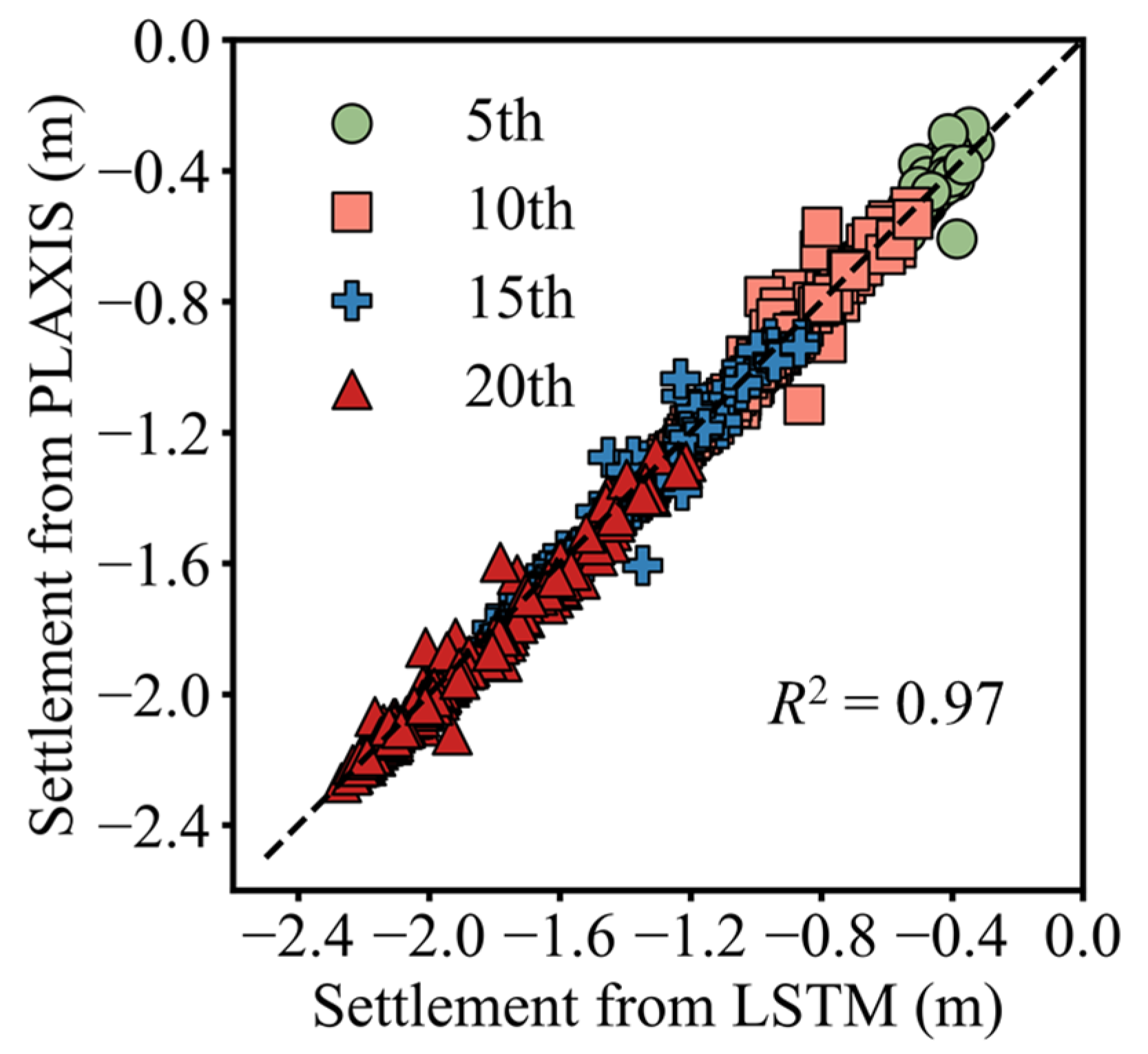
Figure 5 shows the comparison of the settlements calculated from the finite element model and the surrogate LSTM at the 5th, 10th, 15th, and 20th measurement time points. The LSTM model achieves an average coefficient of determination (R2) of 0.97, with most data points closely aligned along the diagonal, indicating high predictive accuracy. This suggests that the model can serve as a surrogate for finite element analysis as the forward model in ES-MDA.

4. Results and Discussion

4.1. Updated Soil Parameters

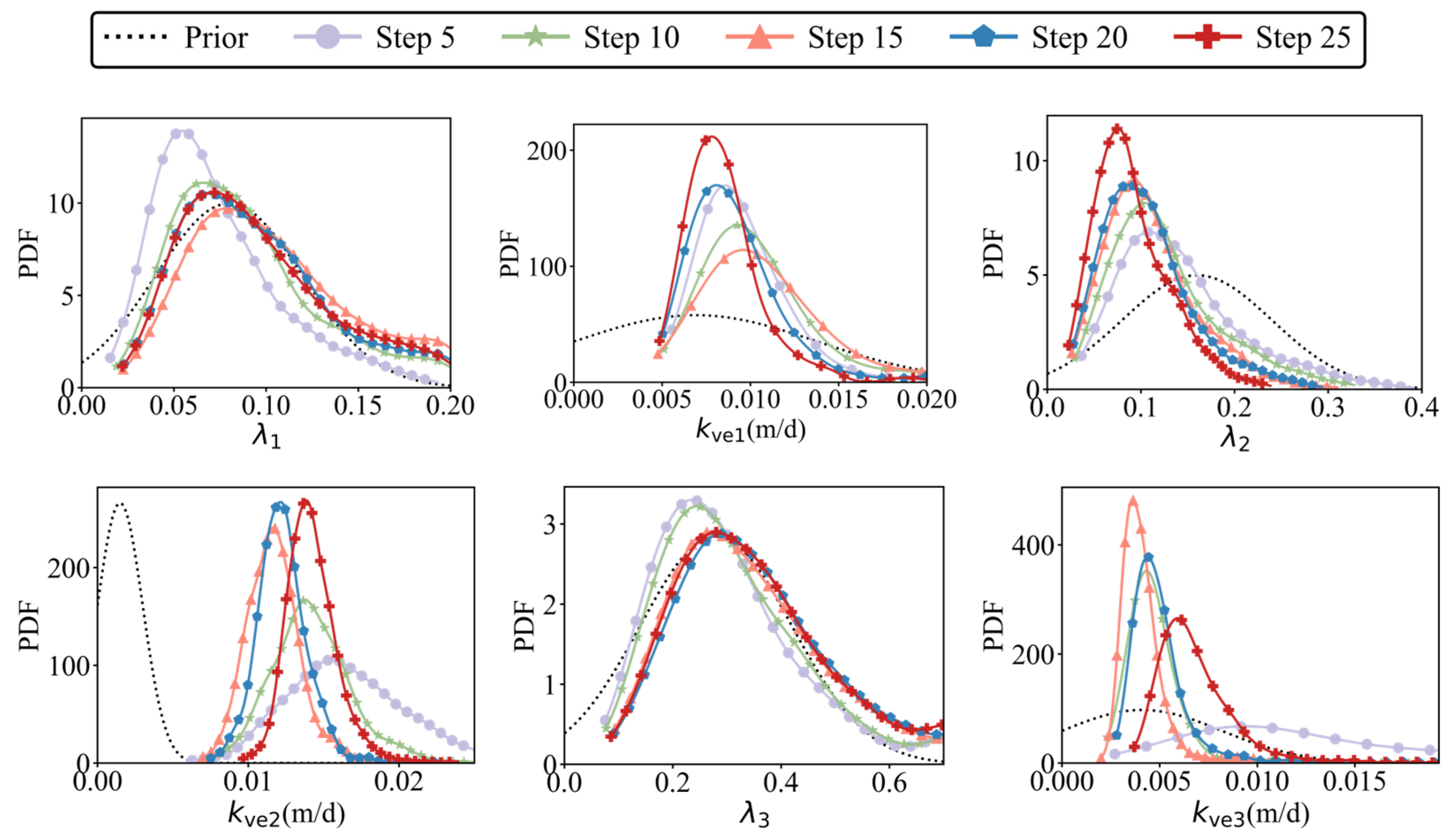
This subsection shows the results of updated soil parameters, which are used as the updated quantities for settlement prediction in the next Section 4.2. Figure 6 shows the updating process of the probability density functions (PDFs) for the compression parameters (λ1 ~ λ5) and the equivalent vertical permeability coefficients (kve1 ~ kve4) over a time sequence (Steps = 0, 5, 10, 15, 20, and 25). By comparing the characteristics of the prior distribution (Step 0) with those of the posterior distributions, it is observed that the posterior PDF curves are generally more concentrated and narrower in range than the prior ones. The posterior distributions of λ2, λ4, and λ5 exhibit a noticeable leftward shift, suggesting that the mean values of their prior distributions are overestimated, indicating that the use of the compression index Cc divided by 2.3 is overly large in this case. The PDFs of the equivalent vertical permeability coefficients (kve) show significant changes. The mean values of the prior distributions for kve are generally smaller than those of the posterior distributions, indicating that the equivalent vertical permeability coefficients (kve) derived from laboratory test data are generally underestimated, i.e., the drainage capacity is underestimated. This discrepancy is mainly attributed to the relatively small size of oedometer specimens and the inevitable sampling disturbance. These factors make it difficult to capture macro-structural features of in situ soils (such as fissures, root channels, and local sand lenses), which in turn leads to an underestimation of the effective drainage capacity. In addition, the prior equivalent permeability coefficients (kve) are usually determined using simplified transformation equations and averaging assumptions, which overlook the complex real effects of PVD spacing, smear zones, construction disturbance, and the spatial heterogeneity of the site. This is particularly evident for kve2, whose posterior PDF curve shifts markedly to larger values compared to the prior, indicating that a higher vertical permeability must be adopted for the corresponding soil layer in the equivalent modeling in order to reasonably reproduce the consolidation rate reflected by the measured settlements. The evolution of the equivalent vertical permeability coefficients varies among soil layers. The top weathered crust (TC) is a relatively dense and low compressibility layer; for this layer, the updated kve1 mainly shows a reduction in uncertainty after data assimilation, while the change in the mean value is limited. The silty clay (SC1) layer overlies the thick soft soil and exerts a certain control on the overall drainage path and deformation. The corresponding kve2 increases significantly during the assimilation process, indicating that the prior conditions underestimated the effective drainage capacity of this layer in the actual project. The mucky clay (MC) layer is the main highly compressible soft clay layer, where excess pore water pressure is dissipated through additional drainage paths after PVD improvement. Although the corresponding kve3 does not exhibit a mean shift as pronounced as that of kve2, its posterior distribution becomes significantly more concentrated. The permeability coefficient kve4 of the lower mucky silty clay (MSC) layer also shows a progressively narrowed distribution, indicating that the uncertainty is reduced by incorporating more data. The updated profile of the equivalent vertical permeability is more consistent with the soil stratification characteristics and the drainage conditions under PVD improvement.

4.2. Settlement Prediction

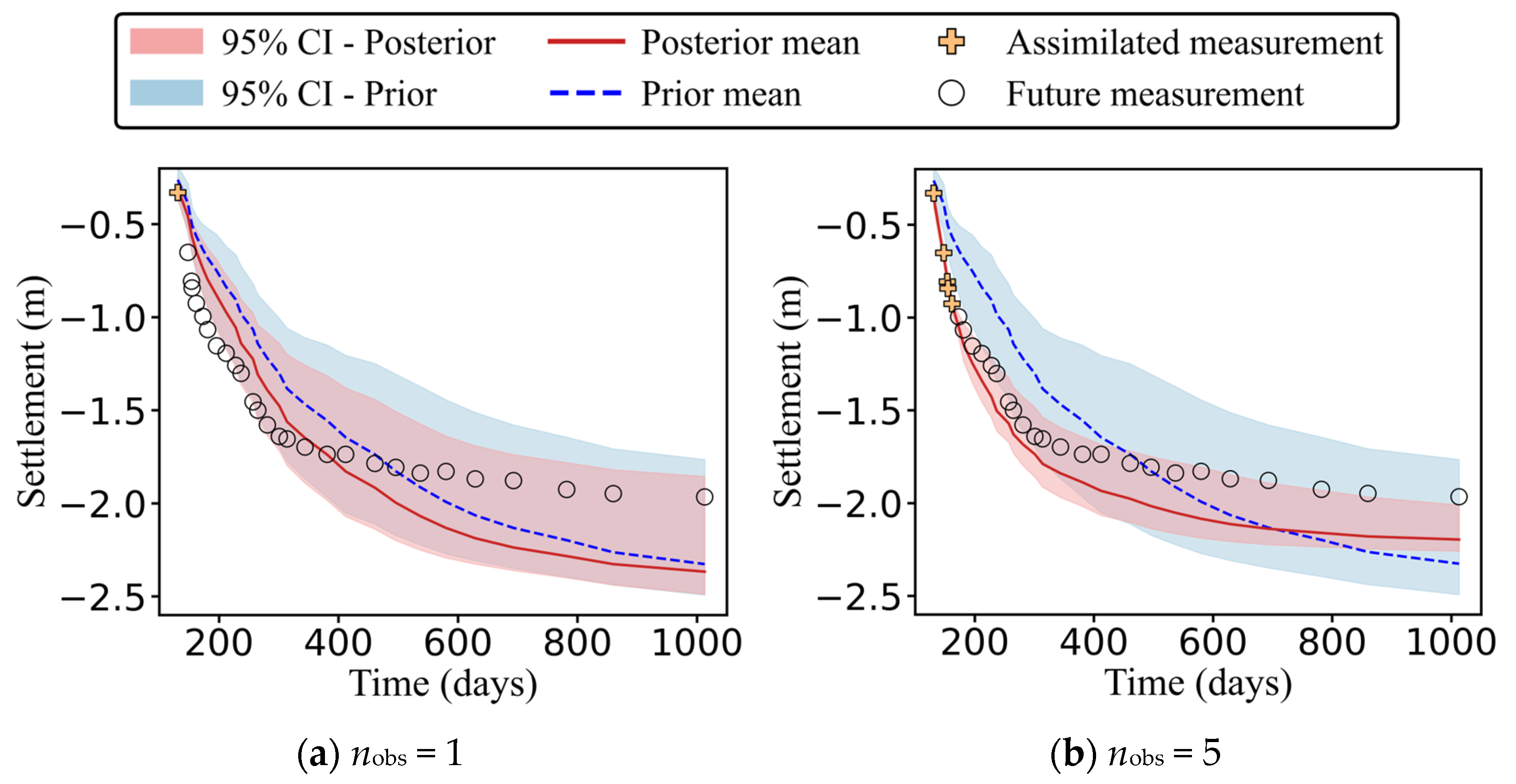
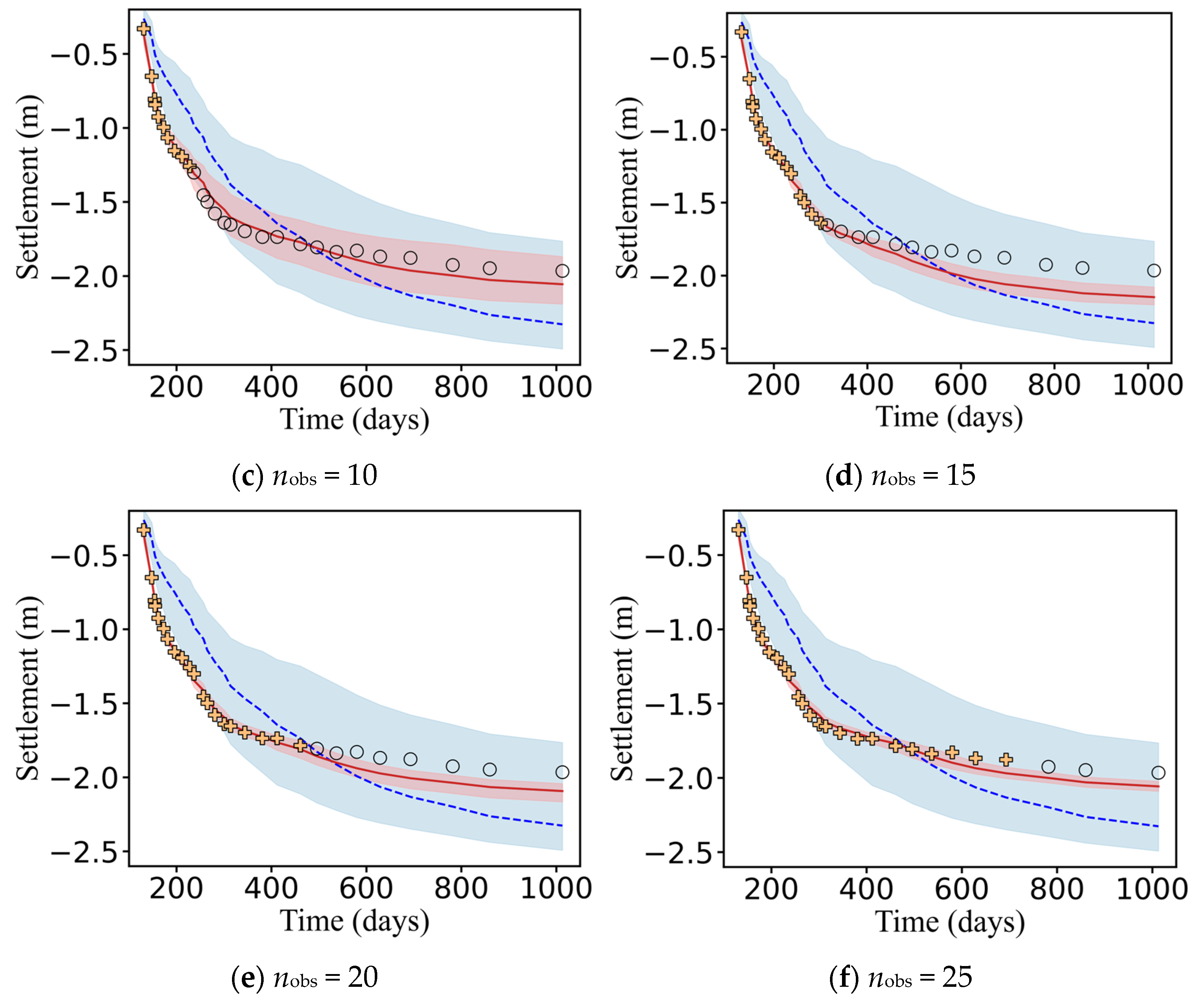
Figure 7 illustrates the updating process of settlement predictions as the number of observations increases. Figure 7a–f present the settlement predictions using posterior samples of soil parameters after progressively assimilating 1, 5, 10, 15, 20, and 25 observation data points, respectively, and compare them with predictions based on the prior distribution of soil parameters. The results indicate that settlement predictions based on the prior distribution exhibit a wide 95% credible interval (CI). For instance, when predicting long-term settlement on the 1000th day, the 95% CI ranges from 1.7 m to 2.5 m, reflecting substantial uncertainty. Moreover, there is a significant deviation between the prior predictive mean (represented by the blue dashed line) and the measurements (represented by circles). As observation data are progressively assimilated, the deviation between the posterior predictive mean (red solid line) and the measurements decreases, and the 95% CI gradually narrows. Specifically, after incorporating 5 observations, the deviation between the predicted mean and the measurements is notably reduced. When the number of observations increases to 10, the predicted mean closely aligns with the measurements. However, with 15 observations, the deviation increases slightly due to a sudden rise in settlement rate at the 11th observation point, which leads to an overestimation in subsequent predictions. As more observations are incorporated (e.g., 20 and 25 points), the deviation again decreases, and the credible interval becomes narrower.
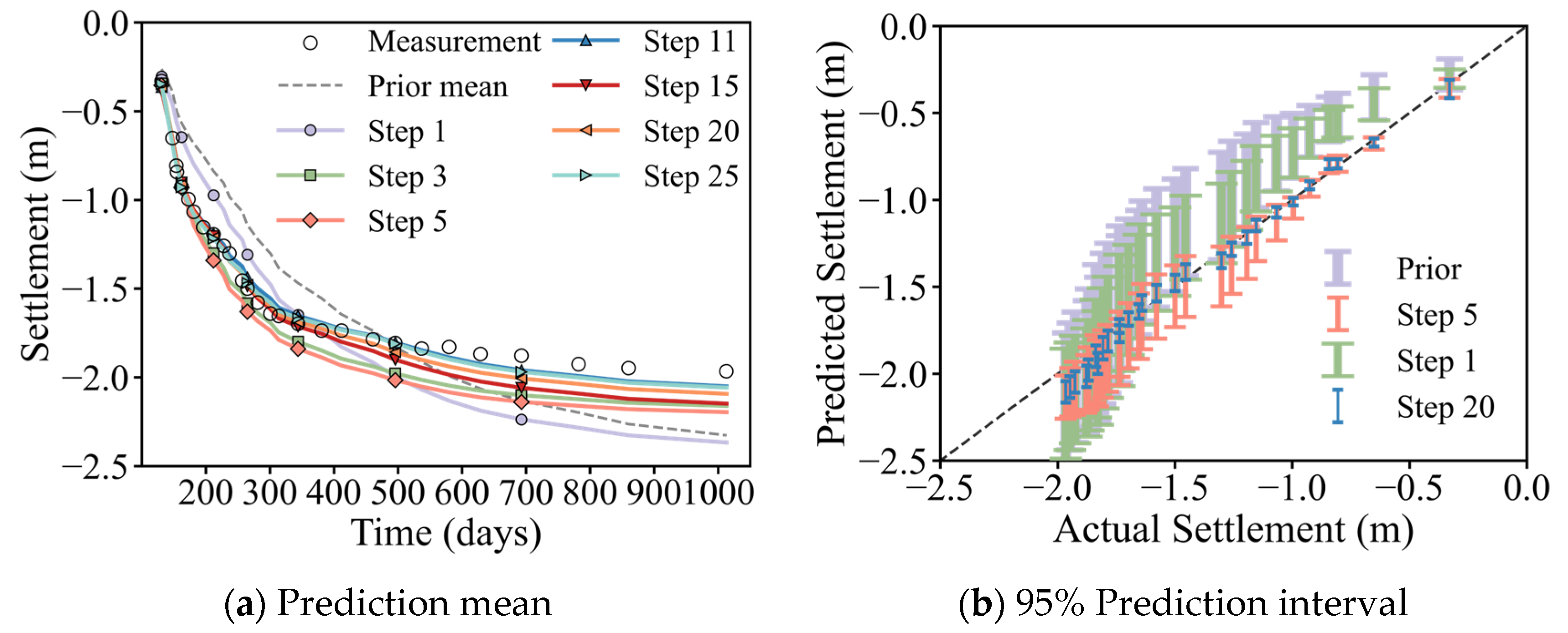
Figure 8 illustrates the influence of the amount of monitoring data on settlement prediction. Figure 8a presents the mean predicted settlements corresponding to different levels of data assimilation. The mean predictions based on the prior distribution and the posterior distribution from Step 1 both show significant deviations from the observed values. In general, as more monitoring data are assimilated, the agreement between the predicted mean and the measured settlements progressively improves, with the most noticeable enhancement occurring during the assimilation of the initial few monitoring points. Notably, the prediction error at the 15th stage is increased compared to the 11th stage. This is due to a sudden variation in the settlement rate after the 11th stage. Figure 8b displays the 95% prediction intervals under varying quantities of monitoring data. When only the prior distribution of soil parameters or a small number of initial measurements are used, the prediction intervals are primarily located in the upper-left region of the diagonal line, indicating a general underestimation of actual settlements. As additional monitoring data are assimilated, the prediction intervals shift closer to the diagonal line, and their width narrows considerably, reflecting a substantial reduction in both prediction bias and uncertainty.
Figure 9 quantitatively analyzes the convergence behavior of the predicted settlement at the 28th monitoring time (Day 1013) throughout the data assimilation process, showing the posterior mean and its 95% CI. In the early stages of assimilation (up to 11 monitoring points), the posterior mean gradually approaches the observed value, although the confidence intervals remain relatively wide. As more data are assimilated (≥11 monitoring points), the width of the confidence interval tends to stabilize; however, the posterior mean begins to deviate from the measured value. After the 15th monitoring point, the posterior mean progressively converges toward the observation once again. Notably, the deviation in the posterior mean between the 11th and 15th monitoring times coincides with the spike in prediction error observed in the corresponding steps in Figure 7a.
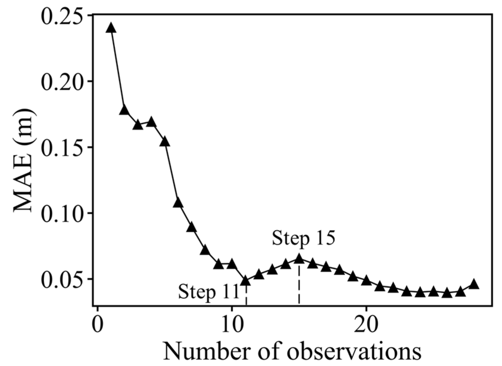
Figure 10 illustrates the influence of the number of observations on the settlement prediction error. The mean absolute error (MAE) is adopted as the evaluation metric, defined as MAE = 1 m n i = 1 m t = 1 n ( y i , t d t ) , where m (m = 500) is the total number of samples, n is the number of observations, yi,j denotes the predicted value, and dj is the measured value. The results indicate that at the initial stage (i.e., upon assimilation of the first observation), the settlement prediction error decreases markedly, confirming the preliminary effectiveness of data assimilation. As the number of observations increases, the prediction error generally shows a decreasing trend and reaches a local minimum after the assimilation of 11 observations. Subsequently, a temporary increase in MAE is observed between the 11th and 15th observations, and a local peak occurs at Step 15. This local increase is consistent with the behaviour shown in Figure 7, where the actual settlement rate exhibits an abrupt rise at the 11th monitoring point. When 11~15 observations are assimilated, the ES-MDA updating learns from this short high-rate stage, so that the updated parameters reproduce this transient behaviour but slightly overestimate the settlements at other times, leading to a larger mean absolute error at these steps. Following the assimilation of 15 observations, the error decreases again as the settlement rate gradually stabilizes.

4.3. Discussion

The results of this study show that the proposed ES-MDA-based settlement prediction method can effectively incorporate field monitoring data to update the probability distributions of soil properties, leading to improved settlement predictions for the embankment. Compared with the prior parameters derived from laboratory tests and empirical formulas, the posterior distributions of the compression index λ and the equivalent vertical hydraulic conductivity kve become noticeably narrower, and their mean values also shift. By assimilating monitoring data within a probabilistic framework, the proposed method corrects the biases in soil parameters and quantifies the associated uncertainties.
From an engineering perspective, the uncertainty bounds of long-term settlement predictions are significantly reduced after data assimilation, and the agreement between the predicted mean settlement and the measured settlement is improved. This improvement becomes evident even when only a limited amount of early monitoring data has been assimilated. Such reliable predictions can support engineering decisions such as adjusting the crest elevation, optimizing the height and duration of preloading, and assessing long-term settlement control and safety margins. The LSTM surrogate model produces settlement predictions that approximate those of the finite element model while substantially reducing computational cost. Integrating the LSTM surrogate model into ES-MDA accelerates the data assimilation process and makes multiple parameter updates and even real-time prediction corrections feasible in practical applications.
The proposed method has several limitations that require further investigation. First, the current framework only assimilates settlement data from the embankment and does not incorporate other monitoring information, such as pore water pressure or lateral displacement. Future work may explore the effects of integrating multi-source observations. Second, from the numerical modeling perspective, the present study employs a two-dimensional model, which is only appropriate for embankments that satisfy the plane strain assumption; three-dimensional modeling would be required for more general geometries. In addition, the Modified Cam Clay model is adopted to represent the behaviour of soft clay, whereas more advanced constitutive models specifically developed for soft soils, such as the soft-clay creep (SCC) model, could be considered in future studies.

5. Conclusions

This study proposes a probabilistic prediction method for embankment settlements based on the ensemble smoother with multiple data assimilation (ES-MDA). The soil properties are updated by incorporating the field monitoring data, and their associated uncertainties are also quantified. An LSTM surrogate model is integrated to enhance the computational efficiency of the assimilation process. The applicability of the proposed method for parameter updating and settlement prediction is evaluated using an embankment constructed on PVD-improved soft ground in Zhejiang, China. The core of this work lies in integrating engineering experience, laboratory test results, and field monitoring data within a Bayesian framework to develop a settlement prediction approach that simultaneously emphasizes accuracy and uncertainty quantification. The main conclusions are as follows:
(1)
In terms of parameter updating, ES-MDA can adaptively refine key consolidation parameters, including the compression index λ and the equivalent vertical permeability kve of each soil layer, by progressively assimilating field monitoring data. Compared with the prior parameters derived from limited oedometer tests and empirical estimates, the posterior probability density functions become more concentrated, and their means exhibit significant shifts, indicating biases in the initial parameter values. The prior mean compression index λ obtained from laboratory tests tends to be overestimated, whereas the prior mean vertical permeability tends to be underestimated. After ES-MDA updating, both compressibility and drainage capacity are adjusted in a manner more consistent with the observed settlement response, and the uncertainty in the parameters is significantly reduced, providing a more reliable basis for subsequent settlement prediction.
(2)
Regarding settlement prediction and uncertainty characterization, ES-MDA effectively exploits early-stage monitoring data to substantially improve long-term settlement prediction performance. Predictions based on prior parameters exhibit a wide 95% prediction interval and a pronounced bias between the predicted mean settlements and the measured values. After assimilating a limited number of observations, the agreement between the predicted mean and the monitoring history improves markedly, and the prediction interval narrows significantly, leading to reduced bias and uncertainty. As more observations are assimilated, prediction errors may exhibit slight and localized increases at certain stages; however, the overall prediction accuracy and stability are considerably superior to those based on the prior parameters. This indicates that, while preserving physical interpretability, the proposed method can provide robust long-term settlement predictions for embankments on soft soil.
(3)
The influence of monitoring data volume and the sensitivity of the method are studied. As the number of assimilated observations increases, the settlement prediction error generally decreases and gradually stabilizes, although a local error peak appears when the number of assimilated monitoring points lies between 11 and 15. This behavior is closely related to the abrupt increase in the settlement rate at the 11th monitoring time. To reproduce this short-term high settlement rate, ES-MDA updates the soil properties accordingly, resulting in an overestimation of settlements at other stages. As subsequent observations are assimilated, the settlement rate returns to a more moderate level, the predicted mean settlements move back towards the measured values, the errors decrease again, and the width of the prediction intervals remains stable. This behavior demonstrates that ES-MDA is sensitive to abrupt changes in ground response, which is beneficial for identifying changes in loading or boundary conditions, but also implies that short-term anomalous monitoring data should be interpreted and used for parameter updating with careful consideration of field conditions.

Author Contributions

P.Z.: Methodology, Writing—Review and editing. Z.Z.: Conceptualization, Writing—Review and editing. D.M.: Formal analysis. X.P.: Methodology, Software, Writing—original draft. F.W.: Methodology, Writing—Review and editing. M.W.: Validation, Supervision. All authors have read and agreed to the published version of the manuscript.

Funding

This work was supported by the Major Science and Technology Program of the Zhejiang Provincial Department of Water Resources (Grant No. RA2211).

Institutional Review Board Statement

Not applicable.

Informed Consent Statement

Not applicable.

Data Availability Statement

The original contributions presented in this study are included in the article. Further inquiries can be directed to the corresponding author.

Conflicts of Interest

Authors Pan Zhao, Delian Ma, Fan Wu and Mingyuan Wang were employed by the company Power China Huadong Engineering Co., Ltd. The remaining authors declare that the research was conducted in the absence of any commercial or financial relationships that could be construed as a potential conflict of interest.

References

  1. Li, C. A simplified method for prediction of embankment settlement in clays. J. Rock Mech. Geotech. Eng. 2014, 6, 61–66. [Google Scholar] [CrossRef]
  2. Park, H.I.; Kim, K.S.; Kim, H.Y. Field performance of a genetic algorithm in the settlement prediction of a thick soft clay deposit in the southern part of the Korean peninsula. Eng. Geol. 2015, 196, 150–157. [Google Scholar] [CrossRef]
  3. Ghosh, B.; Fatahi, B.; Khabbaz, H.; Nguyen, H.H.; Kelly, R. Field study and numerical modelling for a road embankment built on soft soil improved with concrete injected columns and geosynthetics reinforced platform. Geotext. Geomembr. 2021, 49, 804–824. [Google Scholar] [CrossRef]
  4. Venda Oliveira, P.J.; Araújo Santos, L.M.; Almeida e Sousa, J.N.V.; Lemos, L.J.L. Effect of initial stiffness on the behaviour of two geotechnical structures: An embankment and a tunnel. Comput. Geotech. 2021, 136, 104181. [Google Scholar] [CrossRef]
  5. Müthing, N.; Zhao, C.; Hölter, R.; Schanz, T. Settlement prediction for an embankment on soft clay. Comput. Geotech. 2018, 93, 87–103. [Google Scholar] [CrossRef]
  6. Tang, C.; Phoon, K.-K.; Yuan, J.; Tao, Y.; Sun, H. Variability in Geostructural Performance Predictions. ASCE-ASME J. Risk Uncertain. Eng. Syst. Part A Civ. Eng. 2025, 11, 03124003. [Google Scholar] [CrossRef]
  7. Tang, C.; Phoon, K.-K. Model Uncertainties in Foundation Design; Taylor & Francis Group: Abingdon, UK, 2021. [Google Scholar]
  8. Tao, Y.; Zeng, S.; Ying, T.; Sun, H.; Pan, S.; Cai, Y. A deep transfer learning model for the deformation of braced excavations with limited monitoring data. J. Rock Mech. Geotech. Eng. 2025, 17, 1555–1568. [Google Scholar] [CrossRef]
  9. Tao, Y.; Phoon, K.-K.; Sun, H.; Ching, J. Variance reduction function for a potential inclined slip line in a spatially variable soil. Struct. Saf. 2024, 106, 102395. [Google Scholar] [CrossRef]
  10. Cami, B.; Javankhoshdel, S.; Phoon, K.-K.; Ching, J. Scale of Fluctuation for Spatially Varying Soils: Estimation Methods and Values. ASCE-ASME J. Risk Uncertain. Eng. Syst. Part A Civ. Eng. 2020, 6, 03120002. [Google Scholar] [CrossRef]
  11. Phoon, K.-K.; Kulhawy, F.H. Evaluation of geotechnical property variability. Can. Geotech. J. 1999, 36, 625–639. [Google Scholar] [CrossRef]
  12. Ching, J.; Wu, T.-J. Probabilistic transformation models for preconsolidation stress based on clay index properties. Eng. Geol. 2017, 226, 33–43. [Google Scholar] [CrossRef]
  13. Ching, J.Y.; Lin, G.H.; Chen, J.R.; Phoon, K.K. Transformation models for effective friction angle and relative density calibrated based on generic database of coarse-grained soils. Can. Geotech. J. 2017, 54, 481–501. [Google Scholar] [CrossRef]
  14. Kelly, R.B.; Sloan, S.W.; Pineda, J.A.; Kouretzis, G.; Huang, J. Outcomes of the Newcastle symposium for the prediction of embankment behaviour on soft soil. Comput. Geotech. 2018, 93, 9–41. [Google Scholar] [CrossRef]
  15. Doherty, J.P.; Gourvenec, S.; Gaone, F.M.; Pineda, J.A.; Kelly, R.; O’Loughlin, C.D.; Cassidy, M.J.; Sloan, S.W. A novel web based application for storing, managing and sharing geotechnical data, illustrated using the national soft soil field testing facility in Ballina, Australia. Comput. Geotech. 2018, 93, 3–8. [Google Scholar] [CrossRef]
  16. Zeng, S.; Wang, G.; Sun, H.; Tao, Y.; Pan, X. A semi-supervised dual-path model for underground defect detection. Eng. Appl. Artif. Intell. 2025, 158, 111493. [Google Scholar] [CrossRef]
  17. Tao, Y.; Zeng, S.; Sun, H.; Cai, Y.; Zhang, J.; Pan, X. A spatiotemporal deep learning method for excavation-induced wall deflections. J. Rock Mech. Geotech. Eng. 2024, 16, 3327–3338. [Google Scholar] [CrossRef]
  18. Lo, M.K.; Loh, D.R.D.; Chian, S.C.; Ku, T. Probabilistic Prediction of Consolidation Settlement and Pore Water Pressure Using Variational Autoencoder Neural Network. J. Geotech. Geoenviron. Eng. 2023, 149, 04022119. [Google Scholar] [CrossRef]
  19. Lin, S.-S.; Zhang, N.; Zhou, A.; Shen, S.-L. Time-series prediction of shield movement performance during tunneling based on hybrid model. Tunn. Undergr. Space Technol. 2022, 119, 104245. [Google Scholar] [CrossRef]
  20. Siddiqui, F.; Sargent, P.; Montague, G. The use of PCA and signal processing techniques for processing time-based construction settlement data of road embankments. Adv. Eng. Inform. 2020, 46, 101181. [Google Scholar] [CrossRef]
  21. Lo, M.K.; Leung, Y.F. Bayesian updating of subsurface spatial variability for improved prediction of braced excavation response. Can. Geotech. J. 2019, 56, 1169–1183. [Google Scholar] [CrossRef]
  22. Huang, J.; Zeng, C.; Kelly, R. Back analysis of settlement of Teven Road trial embankment using Bayesian updating. Georisk Assess. Manag. Risk Eng. Syst. Geohazards 2019, 13, 320–325. [Google Scholar] [CrossRef]
  23. Qi, X.-H.; Zhou, W.-H. An efficient probabilistic back-analysis method for braced excavations using wall deflection data at multiple points. Comput. Geotech. 2017, 85, 186–198. [Google Scholar] [CrossRef]
  24. Murakami, A.; Shinmura, H.; Ohno, S.; Fujisawa, K. Model identification and parameter estimation of elastoplastic constitutive model by data assimilation using the particle filter. Int. J. Numer. Anal. Methods Geomech. 2017, 42, 110–131. [Google Scholar] [CrossRef]
  25. Huang, S.; Huang, J.; Kelly, R.; Jones, M.; Kamruzzaman, A.H.M. Predicting settlement of embankments built on PVD-improved soil using Bayesian back analysis and elasto-viscoplastic modelling. Comput. Geotech. 2023, 157, 105323. [Google Scholar] [CrossRef]
  26. Tao, Y.; Sun, H.; Cai, Y. Predictions of Deep Excavation Responses Considering Model Uncertainty: Integrating BiLSTM Neural Networks with Bayesian Updating. Int. J. Geomech. 2022, 22, 04021250. [Google Scholar] [CrossRef]
  27. Tian, H.; Cao, Z.; Li, D.; Du, W.; Zhang, F. Efficient and flexible Bayesian updating of embankment settlement on soft soils based on different monitoring datasets. Acta Geotech. 2021, 17, 1273–1294. [Google Scholar] [CrossRef]
  28. Kelly, R.; Huang, J. Bayesian updating for one-dimensional consolidation measurements. Can. Geotech. J. 2015, 52, 1318–1330. [Google Scholar] [CrossRef]
  29. Amavasai, A.; Tahershamsi, H.; Wood, T.; Dijkstra, J. Data assimilation for Bayesian updating of predicted embankment response using monitoring data. Comput. Geotech. 2024, 165, 105936. [Google Scholar] [CrossRef]
  30. Tao, Y.; Pan, S.; Sun, H.; Cai, Y.; Zhang, G.; Sun, M. A bi-fidelity inverse analysis method for deep excavations considering three-dimensional effects. Int. J. Numer. Anal. Methods Geomech. 2024, 48, 2471–2492. [Google Scholar] [CrossRef]
  31. Tao, Y.; Sun, H.; Cai, Y. Bayesian inference of spatially varying parameters in soil constitutive models by using deformation observation data. Int. J. Numer. Anal. Methods Geomech. 2021, 45, 1647–1663. [Google Scholar] [CrossRef]
  32. Tao, Y.; Sun, H.; Cai, Y. Predicting soil settlement with quantified uncertainties by using ensemble Kalman filtering. Eng. Geol. 2020, 276, 105753. [Google Scholar] [CrossRef]
  33. Liu, K.; Vardon, P.J.; Hicks, M.A. Sequential reduction of slope stability uncertainty based on temporal hydraulic measurements via the ensemble Kalman filter. Comput. Geotech. 2018, 95, 147–161. [Google Scholar] [CrossRef]
  34. Vardon, P.J.; Liu, K.; Hicks, M.A. Reduction of slope stability uncertainty based on hydraulic measurement via inverse analysis. Georisk Assess. Manag. Risk Eng. Syst. Geohazards 2016, 10, 223–240. [Google Scholar] [CrossRef]
  35. Hommels, A.; Murakami, A.; Nishimura, S.-I. Comparison of the Ensemble Kalman filter with the Unscented Kalman filter: Application to the construction of a road embankment. In Proceedings of the 19th European Young Geotechnical Engineers Conference, Gyor, Hungary, 3–6 September 2008; pp. 52–54. [Google Scholar]
  36. Evensen, G.; van Leeuwen, P.J. An Ensemble Kalman Smoother for Nonlinear Dynamics. Mon. Weather Rev. 2000, 128, 1852–1867. [Google Scholar] [CrossRef]
  37. van Leeuwen, P.J.; Evensen, G. Data Assimilation and Inverse Methods in Terms of a Probabilistic Formulation. Mon. Weather Rev. 1996, 124, 2898–2913. [Google Scholar] [CrossRef]
  38. Emerick, A.A.; Reynolds, A.C. Ensemble smoother with multiple data assimilation. Comput. Geosci. 2013, 55, 3–15. [Google Scholar] [CrossRef]
  39. Juang, C.H.; Luo, Z.; Atamturktur, S.; Huang, H.W. Bayesian Updating of Soil Parameters for Braced Excavations Using Field Observations. J. Geotech. Geoenviron. Eng. 2013, 139, 395–406. [Google Scholar] [CrossRef]
  40. Iglesias, M.A.; Law, K.J.H.; Stuart, A.M. Evaluation of Gaussian approximations for data assimilation in reservoir models. Comput. Geosci. 2013, 17, 851–885. [Google Scholar] [CrossRef]
  41. Zheng, D.; Huang, J.S.; Li, D.Q.; Kelly, R.; Sloan, S.W. Embankment prediction using testing data and monitored behaviour: A Bayesian updating approach. Comput. Geotech. 2018, 93, 150–162. [Google Scholar] [CrossRef]
  42. Emerick, A.A.; Reynolds, A.C. History matching time-lapse seismic data using the ensemble Kalman filter with multiple data assimilations. Comput. Geosci. 2012, 16, 639–659. [Google Scholar] [CrossRef]
  43. Chai, J.-C.; Shen, S.-L.; Miura, N.; Bergado, D.T. Simple Method of Modeling PVD-Improved Subsoil. J. Geotech. Geoenviron. Eng. 2001, 127, 965–972. [Google Scholar] [CrossRef]
  44. Chai, J.; Shrestha, S.; Hino, T.; Ding, W.; Kamo, Y.; Carter, J. 2D and 3D analyses of an embankment on clay improved by soil–cement columns. Comput. Geotech. 2015, 68, 28–37. [Google Scholar] [CrossRef]
  45. Shuku, T.; Murakami, A.; Nishimura S-i Fujisawa, K.; Nakamura, K. Parameter identification for Cam-clay model in partial loading model tests using the particle filter. Soils Found. 2012, 52, 279–298. [Google Scholar] [CrossRef]
  46. Yildiz, A.; Uysal, F. Modelling of anisotropy and consolidation effect on behaviour of sunshine embankment: Australia. Int. J. Civ. Eng. 2016, 14, 83–95. [Google Scholar] [CrossRef]
  47. Muhammed, J.J.; Jayawickrama, P.W.; Ekwaro-Osire, S. Uncertainty Analysis in Prediction of Settlements for Spatial Prefabricated Vertical Drains Improved Soft Soil Sites. Geosciences 2020, 10, 42. [Google Scholar] [CrossRef]
  48. Huang, W.; Fityus, S.; Bishop, D.; Smith, D.; Sheng, D. Finite-Element Parametric Study of the Consolidation Behavior of a Trial Embankment on Soft Clay. Int. J. Geomech. 2006, 6, 328–341. [Google Scholar] [CrossRef]
  49. Ricciardi, K.L.; Pinder, G.F.; Belitz, K. Comparison of the lognormal and beta distribution functions to describe the uncertainty in permeability. J. Hydrol. 2005, 313, 248–256. [Google Scholar] [CrossRef]
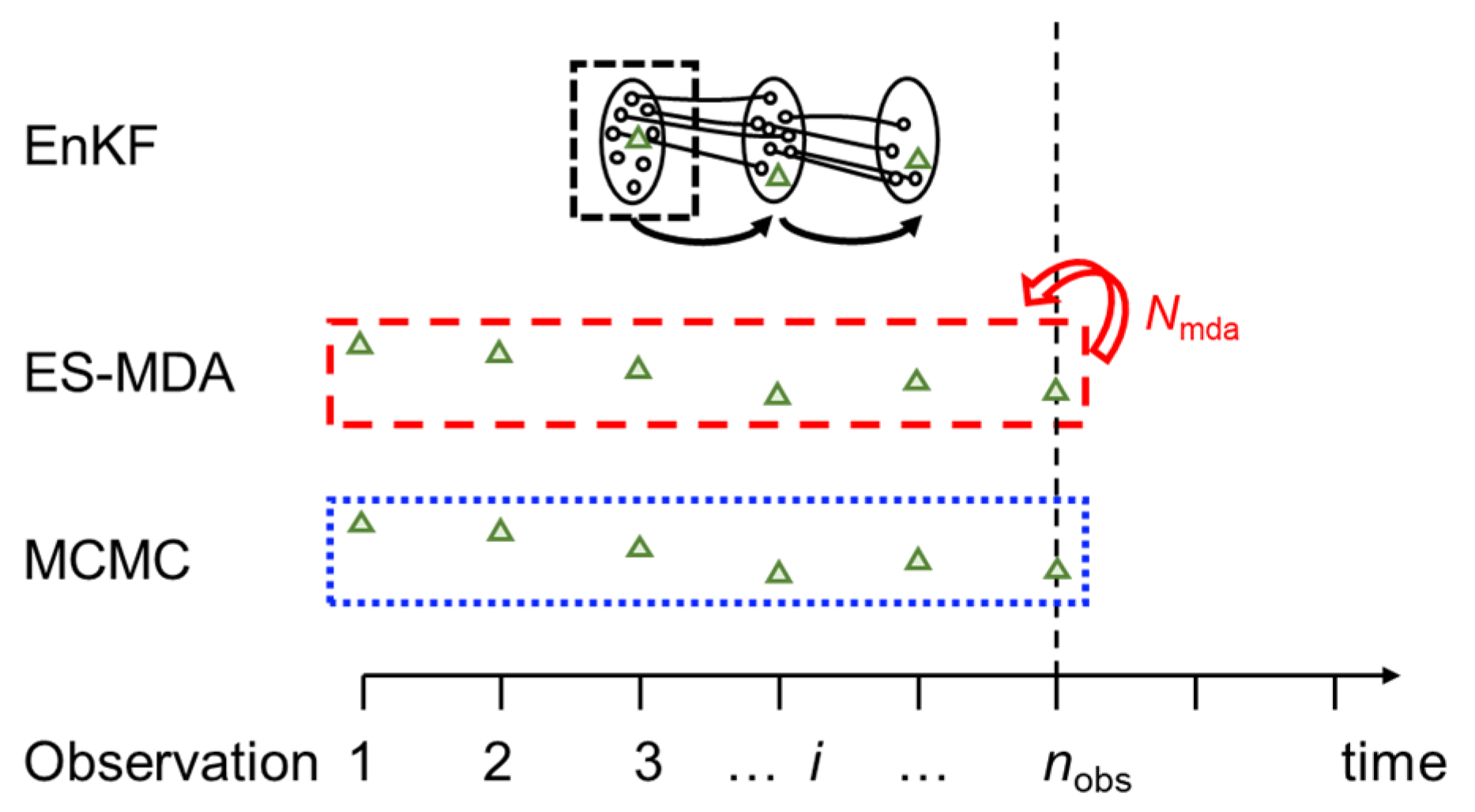
Figure 1. Bayesian updating schemes based on EnKF, ES-MDA, and MCMC.
Applsci 15 13074 g001
Figure 2. Geometry of the trial embankment.
Applsci 15 13074 g002
Figure 3. Embankment construction procedure.
Applsci 15 13074 g003
Figure 4. Diagram of the finite element model (unit: m).
Applsci 15 13074 g004
Figure 5. Comparison of settlements calculated from LSTM and PLAXIS.
Applsci 15 13074 g005
Figure 6. Prior and posterior distributions of random variables.
Applsci 15 13074 g006aApplsci 15 13074 g006b
Figure 7. Settlement predictions using different numbers of observations.
Applsci 15 13074 g007aApplsci 15 13074 g007b
Figure 8. Impact of monitoring data on settlement predictions.
Applsci 15 13074 g008
Figure 9. Settlement predictions at the 1013th day with different amounts of monitoring data.
Applsci 15 13074 g009
Figure 10. Error between all predicted values and observations.
Applsci 15 13074 g010
Table 1. Soil parameters of the project.
Layerγ
(kN/m3)
e0E′
(kPa)
νλκMkh
(10−3 m/d)
kv
(10−3 m/d)
Fill20.0 30,0000.25 32.332.3
TC19.30.81 0.300.080.0081.00.450.54
SC118.51.07 0.350.160.0161.00.090.04
MC17.31.36 0.350.280.0280.80.420.24
MSC17.91.10 0.350.180.0180.80.340.17
SC219.30.81 0.300.10.0101.00.070.03
CS19.5 25,0000.25 4.324.32
Note: TC = top weathered crust; SC = silty clay; MC = very soft mucky clay; MSC = mucky silty clay; CS = clayey sand. Unit weight γ, initial void ratio e0, elastic modulus E′, Poisson’s ratio v, slope of the normal consolidation line λ, slope of the swelling line κ, slope of the critical state line M, horizontal permeability coefficient kh, and vertical permeability coefficient kv.
Table 2. Parameters related to the behavior of PVDs.
ItemSymbolValue
Width (mm)w100
Thickness (mm)t6
Drain spacing (m)SL1.5
Drainage length (m)l19
Drain diameter (mm)dw53
Smear zone diameter (mm)ds355
Ratio of kh over ks in field(kh/ks)f13.5
ds/dws6.7
Diameter of influential zone (m)De1.575
De/dwn29.72
Discharge capacity (m3/a)qw100
Table 3. Prior distribution of random variables.
LayerVariableMeanCoefficient of Variance (COV)Distribution Type
TCλ1 (kPa)0.080.5Lognormal distribution
kve1 (m/d)6.9 × 10−31
SC1λ20.160.5
kve2 (m/d)1.5 × 10−31
MCλ30.280.5
kve3 (m/d)4.1 × 10−31
MSCλ40.180.5
kve4 (m/d)4 × 10−31
SC2λ50.10.5
Table 4. LSTM model settings.
TermValue
Loss functionMSE
Optimization algorithmAdam
Hidden layer2
Hidden dimension128
Learning rate0.001
Batch size16
Epoch100
Disclaimer/Publisher’s Note: The statements, opinions and data contained in all publications are solely those of the individual author(s) and contributor(s) and not of MDPI and/or the editor(s). MDPI and/or the editor(s) disclaim responsibility for any injury to people or property resulting from any ideas, methods, instructions or products referred to in the content.