Featured Application
Deep learning applied to dose distributions with engineered features enables accurate identification of radiotherapy plans requiring patient-specific quality assurance (PSQA). This approach allows more efficient allocation of medical physics staff and linear accelerator time, supporting safer, faster, and more streamlined PSQA workflows.
Abstract
Background: Radiotherapy (RT) is a cornerstone of cancer treatment, with patient-specific quality assurance (PSQA) being essential for patient safety. However, PSQA can be time-consuming, particularly in high-throughput centers. Machine learning and deep learning (DL) offer tools to efficiently analyze large datasets and support data-driven workflows. Methods: DL was applied to predict PSQA outcomes for clinical RT plans delivered with 6 MV and 6 FFF MV. A retrospective dataset of 839 VMAT plans was used to extract 4470 dosiomic features from five automatic isodose contours. The dataset was split into training and test subsets. Two hybrid models were developed to identify plans with γ-passing rates below the median QA value (97%). A prospective dataset of 201 PSQA measurements was used for validation. Results: Both models demonstrated strong predictive performance. In the test set, Hybrid-1 achieved 0.74 specificity and 0.64 sensitivity, while Hybrid-2 reached 0.72 specificity and 0.52 sensitivity. Similar results were observed in the prospective validation cohort. Conclusion: Applying deep learning to dose distributions with carefully engineered features allows accurate identification of RT plans that require PSQA. This approach facilitates more efficient allocation of both personnel and linear accelerator time, thereby supporting safer and more streamlined PSQA workflows.
1. Introduction
As evidenced by the World Health Organization (WHO) [1] the burden due to cancer has been expanding over the years and is predicted to increase by 77% from 2022 to 2050. It was estimated that about 1 in 5 people would develop cancer leading to death, over their entire lifespan: approximately 1 in 9 men and 1 in 12 women. Radiotherapy (RT) has been recognized as an essential element of an effective cancer care program worldwide [2], irrespective of palliative and curative intent, as it can lead to no recurrence in the treated area or symptom relief when lesions have metastasized or grown out of control [3]. Cancer treatment often requires a multidisciplinary approach, leading to the use of RT in combination with surgical intervention and chemotherapy [4].
The need for patient-specific quality assurance (PSQA), driven by technological advancements in RT, has long been central to the allocation of departmental resources. However, in high-throughput centers, the increasing number of patients, as well as the increase in usage of Volumetric Modulated Arc Therapy (VMAT) over simpler techniques, further amplifies the impact of PSQA on the routine workflow of RT departments.
In recent years, artificial intelligence, machine learning, and deep learning have been widely employed to manage and analyze large quantities of data to improve efficacy of procedures using a more comprehensive data-informed approach. Deep neural networks (DNN) and convolutional neural networks (CNN) have been used to predict various aspects of treatment, from diagnosis and the intermediate steps necessary to describe images, to prediction of treatment response and prognosis.
Having algorithms dedicated to the processing of large amounts of features has led to the development of methods that can generate descriptors from all kinds of data. In the field of medical imaging, big data techniques to generate features fall under the umbrella term of radiomics [5] which, when applied to dose distributions, are called dosiomic. The features described in [5] are used to describe first order statistics, as well as the more complex texture properties, of the images from which they are originated. Using a shared set of descriptors aims to standardize and harmonize reporting and investigation of the same kind of images, while having a more straightforward interpretation than the deep features that each DNN builds in the training phase.
The use of dosiomic features in training DNNs and CNNs may lead the deep features to look at different properties of the images, possibly leading to a more complete understanding of the training data.
In this work we have developed a data driven approach based on Deep Learning (DL) algorithms to aid in the identification of the VMAT RT plans which should be checked, to optimize the use of resources by reducing the number of unnecessary PSQA measurements.
To the best of our knowledge, as of writing of this article, this is the first work using an approach based on a 3D convolutional network on absorbed dose distribution in conjunction with dosiomic features that evaluated differences in performance based on the use of flattening filter.
In the following sections, after having briefly described the data available and the neural networks used for the analysis, the results will be presented using confusion matrices and decision curves with increasing levels of pragmatism. Finally, the results will be discussed and compared with the available literature.
2. Materials and Methods
2.1. Input Dataset
The LINACs available to the department are all from Elekta, two VersaHD and one Synergy (Elekta AB, Stockholm, Sweden). The emission spectra of the three LINACs are energy-matched, so they can be considered interchangeable from a treatment delivery standpoint.
VMAT treatment plans were generated in the Pinnacle (version 3) Treatment Planning System (TPS) using the auto-planning engine, employing both flattening filter (FF) and flattening filter-free (FFF) photon beams. Dose calculation was performed in Pinnacle 16.4.3 with a collapsed cone convolution (CCC) algorithm, on a dose grid with isotropic voxel with, most frequently, a side of 3 mm and, occasionally, a side of 2 mm. The instrument used for dosimetry was PTW Octavius 1500 Matrix (PTW-Freiburg, Freiburg, Germany) described in [6].
A total of 1802 dose distributions computed inside the PSQA phantom, acquired from 2021 to 2024 at IRCSS Azienda Ospedaliero-Universitaria di Bologna, were available for this study. All of them had an associated report with the results of the PSQA in terms of γPassingRate and Γ-Index.
The distribution of the γPassingRate over the entire dataset, which is shown in Figure 1, presented a median γPassingRate of 97.6%, an average of 97.2%, and a minimum of 84.7%.
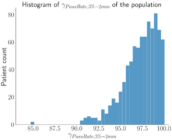
Figure 1.
Distribution of γPassingRate over the entire database.
The threshold to identify safe deliverability of the treatment plans was chosen according to [7] which, in the absence of center-specific values, suggests using γPassingRate > 95% when the Γ-Index is computed with Distance To Agreement (DTA) = 2 mm and a Dose Difference (DD) = 3%, which will be indicated as γ3%,2 mm.
A combined Matlab and R-script was developed to collect the γPassingRate for each patient and plan.
2.2. Model Development and Validation
A general overview of the analysis performed in the study can be seen in Figure 2.

Figure 2.
Flowchart of the analysis.
The input data available to the models was:
- I.
- All the 4470 dosiomic features,
- II.
- The normalized and thresholded 3D dose distribution, originally computed by the Pinnacle3 TPS in the geometry used during the PSQA measurement (i.e., Octavius phantom).
Before developing the model, the dataset was split to use 80% of the data in the training phase, and the remaining 20% for final validation. During the training phase, the dataset has been further randomly subdivided at each epoch to obtain a training dataset (80%) and a testing dataset (20%), which was used to monitor the performance during each epoch.
Two models were developed and investigated, which were called hybrid because both architectures were composed of a fully connected branch, dedicated to the analysis of dosiomic features, and a CNN branch, devoted to the analysis of the 3D dose distributions.
The single branches, with their respective input data, were trained and tested separately to verify that simultaneous usage of both inputs led to an improvement in performance. To ease the presentation of the best results obtained in our research, the results of this analysis are shown in Supplementary Material.
A Python script was developed to automatically pair the γPassingRate from the report to the dose distribution, including only cases in which Γ-Index was computed with DTA = 2 mm and DD = 3% and in which there were no ambiguities in the plan- > report association, such as in cases of second treatments or re-planning. This process reduced the number of available dose distributions to 839, which were stored as couples of DICOM files made up of both RTDose and RTPlan.
Since only dose distributions were used as input, and in order to reduce the time necessary to access these files in memory, all RTDose files have been converted to NRRD format using a bash script for plastimatch [8].
In the conversion phase, to have a homogeneous dataset, all dose distributions have been normalized to the maximum dose and have been thresholded to include only the values > 25% of DMax. This was performed to obtain input images similar to the conditions used in the computation of Γ-Index, which was obtained with global normalization and a 20% dose threshold.
Since the extraction of dosiomic features requires the definition of regions of interest (ROIs), after the conversion, 5 isodose curves were chosen and automatically segmented to prepare for feature extraction. The chosen isodoses were 25%, 50%, 75%, 90% and 95%. These levels were chosen to engineer texture features that describe different regions. Indeed, isodoses of up to 75% are expected to give a general overview of the entire plan while, on the other hand, isodose 90% and 95% were chosen because they contain the steepest gradients, have shapes similar to the actual target and are the regions in which planning objectives are most active giving a large contribution to plan modulation.
The absorbed dose distributions have been further preprocessed during the feature extraction to obtain a wavelet decomposition and the gradient features of the image, using pyradiomics version 3.0.1 [9] on Python 3.11.5 [10].
Overall, each isodose contour was used to extract 894 radiomic features leading to a total of 4470 (=894 × 5) dosiomic features for a single dose distribution. Regardless of the architecture, which are reported in Figure 3, the models were trained to output pass/fail criteria using γPassingRate ≤ 97% as benchmark. This threshold was deliberately selected to prompt the algorithm to detect treatment plans deviating from the median behavior, rather than exclusively flagging those that unequivocally require replanning. An additional advantage of this choice is the creation of a more balanced dataset, albeit at the cost of occasionally recommending PSQA procedures that may ultimately prove unnecessary.
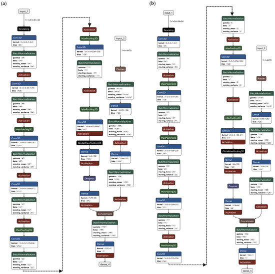
Figure 3.
Architecture of the two main developed models, named (a) Hybrid-1 and (b) Hybrid-2. Left hand branch of architecture is the convolutional neural networks (CNN) trained on computed 3D absorbed dose distribution, right hand branch is the fully connected neural network dedicated to the analysis of radiomic features extracted from the 3D absorbed dose distributions converted from .dcm to .nrrd.
Both models were called hybrid because both architectures are composed of a fully connected branch, dedicated to the analysis of dosiomic features, and a CNN branch, devoted to the analysis of the 3D dose distributions.
The first model, identified as Hybrid-1, had a pooling layer after each convolutional layer and the architecture, which is reported in Figure 3a, had L2 regularization weight set to 0.08, a dropout fraction of 25% and a total of 9.9 million trainable parameters.
The second model, identified as Hybrid-2, had roughly the same number of trainable parameters but two convolutional layers before each pooling, the structure is reported in Figure 3b, with L2 regularization weight left as default and dropout fraction set to 33%.
All the convolutional networks were trained from scratch, instead of using pre-trained network weights, because most of the available networks were trained on 2D images either for object detection or on medical images which were deemed too distant from dose distributions.
Overfitting has been pre-emptively addressed, in all networks, using dropout layers and L2 regularization of both weights and biases, while the risk of exploding and vanishing gradients, as well as stabilization and speed up of training, was addressed with batch normalization layers [11]. All dropout layers have been set to have a 0.3 dropout fraction, all kernels in the convolutional layers were sized as 3 × 3 × 3 tensors with default unitary stride and “same” padding to leave unchanged the dimensions of the distribution before and after a convolution.
Finally, during the training phase, the learning rates of all models have been modified following a policy of reduction on plateaus to give the models the possibility to make finer adjustments along the optimization curve around local minima. The learning rate has been reduced by a factor 0.25, during the training sessions, after 35 successive epochs without improvement in the monitored performance metric. To allow for the changes in the learning rate to have effect, an early stopping policy was defined so that all models stopped once the performance remained on a plateau for more than 75 successive epochs, hence it allowed for at least two reductions in learning rate.
The training process was very time-consuming, mostly due to the lack of ad hoc computational resources. Both hybrid models required from 30 min to 4 h for each training epoch and reached convergence to a suitable performance on the validation dataset after about 150 epochs. For this reason, a more in-depth search for optimal architecture and hyper-parameters was not possible and will be the object of future works.
To reduce the memory space required for the loading dose distributions, while maximizing the amount of information in the volumes, some preprocessing steps have been implemented when loading the data in memory using the tensorflow dataset API [12].
Starting with the normalized and thresholded absorbed dose distributions, the following preprocessing steps were applied:
- Each distribution was cropped to fit within a cube of side length 27 cm, centered on the 25% isodose. The cube size was determined according to the maximum measurable field of the phantom, under standard conditions.
- All distributions were subsequently resampled to matrices of size 94 × 94 × 94. This resolution was selected to minimize the number of resampling operations required across the training set, thereby limiting the introduction of noise arising from artificial alterations of the original dose distributions. These choices, however, limited the range of possible absorbed dose distributions that could be evaluated by the network to those that could be contained by the described cube. There may also be variations in performance of the network when the dimension of pixels in the dose grid used in the TPS differs from 3 mm (e.g., 2 mm).
- The dosiomic features were extracted from the normalized images as well as from their elaboration with a wavelet filter and with a gradient filter, as defined in [9], to emphasize texture and gradients in the dose distributions. The bin width for discretization of the images, prior to feature extraction, was set to 5% to observe variations in dose with that same order of magnitude.
- Finally, before being fed to the networks, all dosiomic features were normalized by subtracting the mean and dividing by the standard deviation across training samples.
The investigated models have been developed in Python using TensorFlow version 2.10 [12].
The performance of the models was evaluated, on the testing dataset, using confusion matrices as well as decision curves [13,14] which conveniently summarized the performances plotting either net benefit or net reduction in interventions for each strategy.
To properly use these curves, it is necessary to decide what an acceptable range of workload, named threshold probability, as the maximum number of QAs the medical physics unit is reasonably willing to perform. A cautious physicist may feel that performing 15–20 QAs to find one error in the machine may be an acceptable use of resources. On the other hand, a physicist with great confidence in the machines available, due to other QA procedures in place, may feel that each PSQA has a large impact on the clinical practice by absorbing too many resources from those required for patients, hence they may deem that even performing 5–10 QAs to find one error may be an acceptable compromise. The first physicist would have a threshold probability of 5–6% (1/20–1/15) while the second would have a threshold probability of 10–20% (1/4–1/3), for this reason the interesting range in which our models had to be evaluated was from roughly 5% to roughly 20% threshold probability.
2.3. Independent Validation of Models
Once trained and tested the entire pipeline was validated prospectively on data acquired routinely in the clinical practice. An additional 201 PSQAs were measured, and the performance was with the same criteria used in the validation phase.
3. Results
3.1. Performance of Models
The training performance with respect to epoch can be seen in Figure 4, in which it can be seen that the Hybrid-1 model took one day and a half to complete 110 epochs, whereas the Hybrid-2 model took, for the same data and number of epochs, 13.5 days.
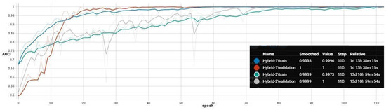
Figure 4.
Training and validation ROC-AUC for both hybrid structures. Plot obtained with Tensorboard.
In Figure 5 and Figure 6, to ease in comparison, other than the confusion matrix for the classifier, a second matrix with actions based on random sampling with a 28.7% frequency was reported.
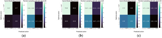
Figure 5.
Hybrid-2 model structure (a) confusion matrix normalized to the total number of plans, i.e., all frequencies sum up to 100%, (b) confusion matrix without normalization, and (c) confusion matrix normalized with respect to the true label. Diagonal elements are true positive and negative rates, while on the anti-diagonal are false positive and negative rates.
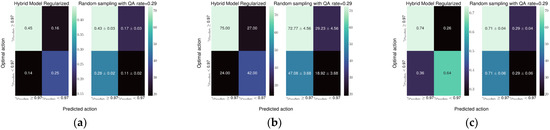
Figure 6.
Hybrid-1 model structure (a) confusion matrix normalized to the total number of plans, i.e., all frequencies sum up to 100%, (b) confusion matrix without normalization, and (c) confusion matrix normalized with respect to the true label. Diagonal elements are true positive and negative rates, while on the anti-diagonal are false positive and negative rates.
By comparing Figure 5 and Figure 6, a slight advantage for the Hybrid-1 structure emerges. With the aid of the matrices obtained with random sampling, which reproduce the current method to choose the PSQA, the hybrid models provide, when used without information about the flattening filter, almost a doubling in the true positive rate and a small reduction in the false negative rate.
Up to this point, the comparison was made with γPassingRate < 97% because that was the benchmark in the training phase, which was chosen to identify plans worse than the median output of the service.
However, from a practical standpoint, another interesting benchmark is the rates in identifying the plans that will obtain a γPassingRate < 95% simultaneously accounting for the use of the flattening filter in the beam.
For this reason, the same testing dataset, made up of 168 plans, was divided according to the use of FF and the performance was assessed on the two sub-groups comparing them against a QA rate of 100% for the FFF plans (103 plans) and 11% for the plans with flattening filter (65 plans). The results of this analysis are reported in Figure 7 and Figure 8.
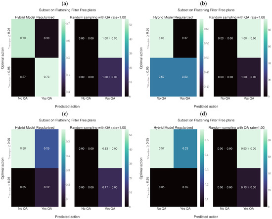
Figure 7.
Performance of the Hybrid-2 architecture. (a) FFF plans, confusion matrix normalized with respect to the true label. Diagonal elements are true positive and negative rates, while on the anti-diagonal are false positive and negative rates. (b) Plans with FF, confusion matrix normalized with respect to the true label. (c) FFF plans, confusion matrix normalized to the total number of plans, i.e., all frequencies sum up to 100%. (d) Plans with FF, confusion matrix normalized to the total number of plans.
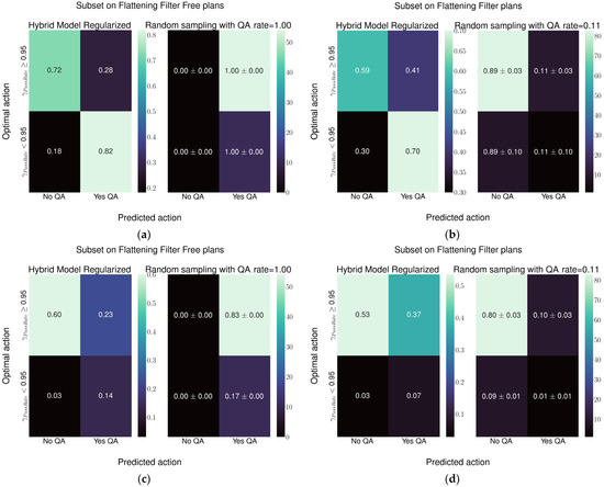
Figure 8.
Results of the Hybrid-1 structure (a) FFF plans, confusion matrix normalized with respect to the true label. Diagonal elements are true positive and negative rates, while on the anti-diagonal are false positive and negative rates. (b) Plans with FF, confusion matrix normalized with respect to the true label. (c) FFF plans, confusion matrix normalized to the total number of plans, i.e., all frequencies sum up to 100%. (d) Plans with FF, confusion matrix normalized to the total number of plans.
Finally, to summarize the performance and highlight in which conditions the networks can be meaningfully used, the decision curves for both classifiers are reported in Figure 9, both as net benefit and net reduction in interventions evaluated regardless of flattening filter using Gamma < 95% as decision limit.
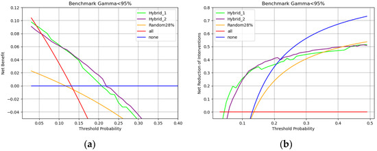
Figure 9.
Decision curves obtained with both hybrid models, evaluated on the testing dataset regardless of flattening filter. (a) Net benefit curve and (b) Net reduction in interventions.
As in the previous figures, when evaluating the models without considering the use of flattening filters, the current practice in our center is to randomly perform 28% of PSQAs, this strategy was included to be compared against both models and against the two extreme strategies of performing all PSQAs and performing none.
The decision curves in Figure 10 are obtained by evaluating the plans when considering the use of the flattening filter. For Figure 10a,b, the competing strategy is performing all PSQAs, whereas the competing strategy for FF plans is a random sampling with frequency 11%, see Figure 10c,d.
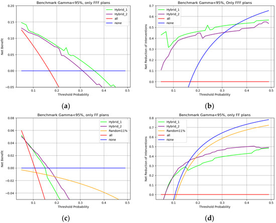
Figure 10.
Decision curves obtained with both hybrid models, developed on the testing dataset without distinguishing between the use or non-use of a flattening filter. Net benefit curves are shown for (a) FFF plans and (c) FF plans. The corresponding net reduction in interventions is shown for (b) FFF plans and (d) FF plans.
3.2. Independent Validation of Models
Once trained and tested the entire pipeline was validated prospectively on newly acquired data. An additional 201 Patient Specific QAs was measured, and the performance was evaluated with the same criteria used in the validation phase. The results, shown in Figures S1 and S2, highlight that performance was in line with those obtained with the retrospectively collected database, leading us to believe that the approach can generally be applied to the plans generated in the center which generated the data used in the training phase.
3.3. Evaluation of Routine Applicability
To evaluate the impact of the model in the routine of the physics department, an ad hoc pipeline was built to perform all the processing necessary from a folder of suitable RTDose files to a report with the final model output.
A summary of the steps performed by the pipeline can be made as follows, considering that these steps are necessary for each patient:
- Conversion from “.dcm” to “.nrrd” to speed up reading the data before inputting it in the model.
- Normalization and threshold of the dose distribution.
- Automatic contouring of the five isodose levels 25%, 50%, 75%, 90%,95%.
- Dosiomic extraction from all five contours.
- Loading model in memory.
- Loading data into memory, preparation of batches and final evaluation.
- Creation of an excel report with the suggested action according to the model.
When tested on a laptop pc with 8 GB of RAM, without GPU and an intel core i7 processor, the hybrid-2 model took 19 min and 36 s for the evaluation of 50 patients, meaning less than 30 s per patient. Out of the entire computation time, 12 min were dedicated to the preprocessing and feature engineering while the remaining 7.5 min were used by the model to produce the final predictions.
In the evaluation of the same 50 patients on the same laptop, the hybrid-1 model took a total 13 min and 42 s meaning 16.5 s per patient. Out of the entire computation time, 12 min and 56 s were dedicated to the preprocessing and feature engineering, while the remaining 46 s were used by the model to produce the final predictions.
Since the times for the preprocessing steps were almost identical, differences in model deployment times are aligned with the performances seen in the training phase and can be attributed to the differences in model architecture.
4. Discussion
This work shows the applicability of the DL approaches on absorbed doses saved in the RTDose files to predict the need to perform the QA procedure of VMAT plans generated using FFF or FF beams.
The best model performance was obtained with the Hybrid-1 model, which reached a specificity of 0.74 and a sensitivity of 0.64 followed by the Hybrid-2 model with a specificity and sensitivity of 0.72 and 0.52, respectively. Both models represent a relevant improvement in the current detection ability of the random sampling used at our institute.
Regarding Hybrid-2 architecture, considering plans employing the 6 MV FFF beam, and in reference to Figure 7c, the current practice of performing the QA for all plans leads to performing 83% of QAs unnecessarily to identify the 17% of plans that need checking. The model would reduce the total QA workload for FFF plans from 100% to 37%, of which 12% would be needed and 25% unnecessary. Considering the plans with the flattening filter, in reference to Figure 7d, the current practice leads to checking, on average, 11% of plans. Over the total number of FF plans, this leads to performing unnecessary QAs in 10% of cases while just 1% of QAs would lead to identification of challenging plans. Using this model would mean performing 38% of QAs, of which 5% would be necessary and 33% unnecessary. This would mean improving the detection of plans needing attention by a factor of five, while increasing the number of unnecessary QAs by a factor of three.
Regarding Hybrid-1 architecture, considering plans employing the 6 MV FFF beam, and in reference to Figure 8c, the current practice of performing the QA for all plans leads to performing 83% of QAs unnecessarily to identify the 17% of plans that need checking. The model would reduce the total QA workload for FFF plans from 100% to 37%, of which 14% would be needed and 23% would be unnecessary. Considering the plans with the flattening filter, in reference to Figure 8d, the current practice leads to checking, on average, 11% of plans. Over the total number of FF plans, this leads to performing unnecessary QAs in 10% of cases while just 1% of QAs would lead to identification of challenging plans. Using the model would mean performing 44% of QAs, of which 7% would be necessary and 37% unnecessary. This would mean improving the detection of plans needing attention by a factor of seven, while increasing the number of unnecessary QAs by a factor three.
Both hybrid models would lead to an increase in total number of QA performed; however, the increase in performed QAs would be exclusively made up of plans under the attention limit suggested by [7].
When considering Figure 9 and Figure 10, net benefit is the percentage of true positives added without increasing true negatives, i.e., the percentage of overall QAs that each model would correctly identify as in need of measurement without adding unnecessary workload. Threshold probability represents a sliding scale that starts, on the left, from feeling that performing all QAs is necessary because missing an error is too dangerous and ends, on the right, with being willing to perform fewer QAs because they are too demanding on clinical routine.
With these considerations in mind Figure 9a shows that a team that is really concerned with possible errors would choose all PSQAs strategy. As the weight of QAs on the routine increases, a team willing to perform no more than 20 PSQAs to find a single error (0.05 threshold probability) would choose the hybrid-1 model. For a team that would perform no more than 10 PSQAs to find a single error (0.1 threshold probability), hybrid-2 would be the preferred model. Finally, for cases in which PSQAs are too expensive and performing more than 5–4 QAs (0.2–0.25% threshold probability) to find a single error becomes unacceptable, the winning strategy becomes performing no PSQA at all. Both hybrid models, when employed in their respective regions of relevance, would lead to a net benefit of 10% to 5%.
On the other hand, Figure 9b shows how many unnecessary PSQAs would be avoided by using each strategy. The Hybrid-1 model is preferred up to threshold probabilities of around 10% and would lead to a reduction in unnecessary workload of 30%. When PSQAs are more demanding, i.e., up to a threshold probability of around 20%, using the Hybrid-2 model would lead to a 40% reduction in unnecessary procedures. If performing five PSQAs to find one error is an unacceptable workload (threshold probability > 0.25%) then the winning strategy to reduce workload is to simply perform no PSQAs (blue line).
In all cases randomly choosing QAs, i.e., yellow lines of Figure 9a,b is the worst available strategy both in the attempt to reduce the workload and with the intention of improving correct identification.
In the case of FFF plans, i.e., Figure 10a,b, the Hybrid-1 structure is always the optimal choice leading to around 10% improvement in net benefit and around a 40% reduction in unnecessary workload.
On the other hand, when considering FF plans, i.e., Figure 10c,d, up to 10% threshold probability Hybrid-1 and Hybrid-2 lead to an equivalent net benefit and reduction in interventions. In cases in which the unnecessary workload of PSQAs is more relevant (thresholds > 10%) Figure 10c,d shows that the Hybrid-2 model would be better both in benefit and for reduction in interventions. In all cases in which QAs are too demanding, the winning strategy is clearly to perform no PSQAs at all. Finally, a random sampling strategy is confirmed to be the worst option available in all cases.
To the authors knowledge, this is the first study that created a model based on the 3D absorbed dose distribution and that evaluated the performance in differentiating between plans with and without flattening filter. It is worth mentioning that all the architectures presented in this work, apart from retraining the weights and changing the activation of the last layer, can be converted to predicting γ3%,2 mm as a raw number. The regression task was initially explored, however, it is not shown in this work because it produced a model with a mean absolute error of 1.5–2% which, given the width of the distributions observed in the available data, would be a performance equivalent to always predicting the average γPassingRate and would lead to an underestimation of risk of failure for the PSQA.
Miao et al. [15] used a similar CNN structure to perform a regression analysis on 2D dose distributions computed in the reference PSQA geometry with different phantom and dose calculation algorithms. The mean absolute errors reported are 1.1%, 1.9%, 1.7%, 2.3% for γ3%,3 mm γ3%,2 mm γ2%,3 mm γ2%,2 mm respectively, which are in line with our initial results on a regression task. Unfortunately, the true and false positive rates are not reported, hence no direct comparison can be made.
Lambri et al. [13] trained a DL model based only on complexity features from 5622 VMAT plans, which was evaluated with an action limit of 95%, in a multicentric setting, obtaining a specificity of 0.90, 0.90 and 0.68, and a sensitivity of 0.61, 0.25, and 0.55, respectively, in the three institutions where it was tested. A direct comparison with their results can be made using the same action limit as [13], Hybrid-1 reaches a sensitivity and specificity of 0.65 and 0.76 while the Hybrid-2 model reaches a sensitivity and specificity of 0.66 and 0.62, respectively.
Huang et al. [14] reported a CNN trained on a dataset of planar dose distributions extracted with the Pylinac library from 556 single fields of intensity-modulated radiation therapy (IMRT) treatments. In predicting γ3%,2 mm they obtained a mean absolute error of 2% whereas, in the classification of plans with γPassingRate < 85%, they reported a 57% sensitivity and a 100% specificity. In their testing set they had less than 9% of plans below their defined action limits, which complicates the comparison and could reduce the robustness of the estimated specificity and sensitivity. It should also be noted that, according to [15], plans with γPassingRate < 0.90 are unfit for clinical delivery, hence rarely seen in our routine measurements.
Li et al. [16] processed the multileaf aperture images of 761 VMAT using 3D-MResNet to predict the γPassingRate at 3%/2 mm and 2%/2 mm. The mean absolute errors of the model for the test set were 1.63% and 2.38% at 3%/2 mm and 2%/2 mm, respectively.
In a classification task with the benchmark chosen with the aid of a cost-sensitive error rate, Li et al. [15] reported, for γ3%,2 mm, a sensitivity of 13/78 ≃ 17%.
Yang et al. [17] and Cui et al. [18] commissioned and deployed a hybrid StarGAN architecture in a multicentric setting involving eight different institutions. Limited to the γ3%,2 mm criteria, they report specificities of 70–75% and sensitivities of 90–92%, with a 2.45% RMSE in the regression task. However, their input was limited to plan complexity features, making direct comparison of performances rather difficult.
As noted in [13], the results are inherently dependent on the specific linear accelerator and detector, which limits the possibility of deriving universally valid conclusions in a single-center setting. Although the model was trained on dose distributions generated by a single TPS, with a specific machine model and detector, its structure and learned representations provide a solid foundation. With appropriate adaptation or fine-tuning, the model could be extended to centers employing different machines, TPSs, or detectors. This aspect will be the focus of future studies aimed at assessing the model’s generalizability and clinical applicability in multicenter scenarios.
There are various possible pathways for future developments. One of the interesting prospects for this approach could be to add a third branch in the network to analyze the RTPlan files. Despite the complexities in properly unpacking the information in RTPlan files, and in designing a network able to analyze said information, it is reasonable to expect an improvement in performance. Given the differences in distributions of γ3%,2 mm due to the district, a further improvement could be obtained by adding clinical information on the plan in the input for the model. Another interesting direction would be to implement a network that produces multiple outputs for various DD and DTA criteria in the Γ-Index computation. This structure would have the advantage of providing a more comprehensive overview of the plan; however, the implementation of this kind of structure would require a large effort in data collection and storage as well as multiple routinary testing in each PSQA event.
A limitation of this study lies in the data partitioning strategy, which relied on per-epoch random 80/20 splits. This approach may introduce generalization bias if multiple plans from the same patient, or plans with nearly identical parameters, are distributed across training and test sets. Future implementations employing fixed patient- or course-level partitions, together with a temporal (year-wise) hold-out informed by PSQA device characteristics and linac performance data, are expected to better assess robustness against potential machine variations or workflow drift, thereby improving the model’s external validity and reproducibility.
Moreover, all the preprocessing steps were aimed at harmonizing the dose distributions and to make them comparable regardless of dose shape, prescription dose, and grid shape for the computation inside the TPS. However, these choices limit the possible sizes of absorbed dose distributions acceptable by the models and are strictly dependent on the maximum sensitive volume of the detector used which, in this work, was dictated by the OCTAVIUS 1500 matrix to be a cylinder of 27 cm in diameter and height. A first example of absorbed dose distributions unseen in training due to available devices, would be those in which a single target extends more than 27 cm, or when more lesions treated simultaneously are separated by more than 27 cm. Another possible limitation could be encountered in analyzing doses computed on a grid with pixel size different from 3 mm (e.g., 1 or 5 mm). Upon implementation each center should choose how to handle these limit cases according to the typical cohorts encountered in the clinical practice.
Finally, the analysis pipeline has not been yet optimized hence the speed and performance in training can still be improved, both by employing ad hoc computational resources and by optimizing the code. Reducing the training times would make re-training the network less expensive, therefore mitigating the risk of not being able to describe slow drifts in the machine performance due to aging or sharp changes after maintenance, which are otherwise guaranteed by the other facets of the QA program.
5. Conclusions
In conclusion, the integration of DL with absorbed dose distributions and optimally engineered features substantially improves the sensitivity in detecting treatment plans that require quality assurance, without a concomitant rise in false positive findings. This approach has the potential to optimize quality assurance workflows and promote a more efficient allocation of resources within the medical physics department.
Supplementary Materials
The following supporting information can be downloaded at: https://www.mdpi.com/article/10.3390/app152312747/s1, Figure S1: Confusion matrix of the top performing model in the a posteriori validation. The frequencies are normalized with respect to the true label which, in this case, is GPR < 95%. Diagonal elements are true positive and negative rates, while on the anti-diagonal are false positive and negative rates. Figure S2: Confusion matrix of the top performing model in the a posteriori validation. The frequencies are normalized with respect to the true label which, in this case, is GPR < 97%. Diagonal elements are true positive and negative rates, while on the anti-diagonal are false positive and negative rates. Figure S3: Confusion matrix for the performance of the fully connected network used with only dosiomic features as input. The frequencies are normalized with respect to the true label which, in this case, is GPR < 97% Figure S4: Confusion matrix for the performance of 3D Convolutional NeuralNetwork using 3D dose distribution as input. The frequencies are normalized with respect to the true label which, in this case, is GPR < 97%.
Author Contributions
Conceptualization, L.S. (Lorenzo Spagnoli) and L.S. (Lidia Strigari); methodology, L.S. (Lorenzo Spagnoli) and L.S. (Lidia Strigari); validation, L.S. (Lorenzo Spagnoli), G.D.G. and S.S.; formal analysis, L.S. (Lorenzo Spagnoli) and M.S.; investigation, L.S. (Lorenzo Spagnoli), M.S., S.S., F.B., I.G., C.M., G.D.G., S.T. and L.S. (Lidia Strigari); data curation, M.S., C.M., I.G., S.S. and L.S. (Lidia Strigari); writing—original draft preparation, L.S. (Lorenzo Spagnoli), M.S., F.B., C.M., S.T., I.G., G.D.G. and S.S.; writing—review and editing, L.S. (Lorenzo Spagnoli) and L.S. (Lidia Strigari); visualization, L.S. (Lorenzo Spagnoli) and L.S. (Lidia Strigari); supervision, L.S. (Lidia Strigari). All authors have read and agreed to the published version of the manuscript.
Funding
This research received no external funding.
Data Availability Statement
The datasets used during the current study are available from the corresponding author on reasonable request.
Conflicts of Interest
The authors declare no conflicts of interest.
Abbreviations
The following abbreviations are used in this manuscript:
| CCC | Collapsed cone convolution |
| CNN | Convolutional neural networks |
| DL | Deep Learning |
| DNN | Deep neural networks |
| DD | Dose Difference |
| DTA | Distance To Agreement |
| FF | Flattening filter |
| FFF | Flattening Filter-Free |
| IMRT | Intensity-modulated radiation therapy |
| PSQA | Patient-specific quality assurance |
| RT | Radiotherapy |
| ROIs | Regions of interest |
| TPS | Treatment planning system |
| VMAT | Volumetric Modulated Arc Therapy |
References
- World Health Organization. Global cancer burden growing, amidst mounting need for services. Saudi Med. J. 2024, 45, 326–327. [Google Scholar]
- Abshire, D.; Lang, M.K. The Evolution of Radiation Therapy in Treating Cancer. Semin. Oncol. Nurs. 2018, 34, 151–157. [Google Scholar] [CrossRef] [PubMed]
- Russell, A.H. Clinical Radiation Oncology. Gynecol. Oncol. 2001, 81, 335. [Google Scholar] [CrossRef]
- Barton, M.B.; Jacob, S.; Shafiq, J.; Wong, K.; Thompson, S.R.; Hanna, T.P.; Delaney, G.P. Estimating the demand for radiotherapy from the evidence: A review of changes from 2003 to 2012. Radiother. Oncol. 2014, 112, 140–144. [Google Scholar] [CrossRef] [PubMed]
- Zwanenburg, A.; Leger, S.; Vallières, M.; Löck, S. Image biomarker standardisation initiative. arXiv 2016, arXiv:1612.07003. [Google Scholar]
- Stelljes, T.S.; Harmeyer, A.; Reuter, J.; Looe, H.K.; Chofor, N.; Harder, D.; Poppe, B. Dosimetric characteristics of the novel 2D ionization chamber array OCTAVIUS Detector 1500. Med. Phys. 2015, 42, 1528–1537. [Google Scholar] [CrossRef] [PubMed]
- Miften, M.; Olch, A.; Mihailidis, D.; Moran, J.; Pawlicki, T.; Molineu, A.; Li, H.; Wijesooriya, K.; Shi, J.; Xia, P.; et al. Tolerance limits and methodologies for IMRT measurement-based verification QA: Recommendations of AAPM Task Group No. 218. Med. Phys. 2018, 45, e53–e83. [Google Scholar] [CrossRef] [PubMed]
- Zaffino, P.; Raudaschl, P.; Fritscher, K.; Sharp, G.C.; Spadea, M.F. Technical Note: Plastimatch mabs, an open source tool for automatic image segmentation. Med. Phys. 2016, 43, 5155. [Google Scholar] [CrossRef] [PubMed]
- Van Griethuysen, J.J.M.; Fedorov, A.; Parmar, C.; Hosny, A.; Aucoin, N.; Narayan, V.; Beets-Tan, R.G.H.; Fillion-Robin, J.C.; Pieper, S.; Aerts, H. Computational Radiomics System to Decode the Radiographic Phenotype. Cancer Res. 2017, 77, e104–e107. [Google Scholar] [CrossRef] [PubMed]
- Van Rossum, G.; Drake, F.L. Python 3 Reference Manual; CreateSpace: Scotts Valley, CA, USA, 2009. [Google Scholar]
- Ioffe, S.; Szegedy, C. Batch normalization: Accelerating deep network training by reducing internal covariate shift. In Proceedings of the 32nd International Conference on Machine Learning, Lille, France, 6–11 July 2015; Volume 37, pp. 448–456. [Google Scholar]
- Abadi, M.; Barham, P.; Chen, J.; Chen, Z.; Davis, A.; Dean, J.; Devin, M.; Ghemawat, S.; Irving, G.; Isard, M.; et al. TensorFlow: A system for large-scale machine learning. In Proceedings of the 12th USENIX Symposium on Operating Systems Design and Implementation, Savannah, GA, USA, 2–4 November 2016. [Google Scholar]
- Lambri, N.; Hernandez, V.; Sáez, J.; Pelizzoli, M.; Parabicoli, S.; Tomatis, S.; Loiacono, D.; Scorsetti, M.; Mancosu, P. Multicentric evaluation of a machine learning model to streamline the radiotherapy patient specific quality assurance process. Phys. Med. 2023, 110, 102593. [Google Scholar] [CrossRef] [PubMed]
- Huang, Y.; Pi, Y.; Ma, K.; Miao, X.; Fu, S.; Chen, H.; Wang, H.; Gu, H.; Shao, Y.; Duan, Y.; et al. Virtual Patient-Specific Quality Assurance of IMRT Using UNet++: Classification, Gamma Passing Rates Prediction, and Dose Difference Prediction. Front. Oncol. 2021, 11, 700343. [Google Scholar] [CrossRef] [PubMed]
- Miao, J.; Xu, Y.; Men, K.; Dai, J. A feasibility study of deep learning prediction model for VMAT patient-specific QA. Front. Oncol. 2025, 15, 1509449. [Google Scholar] [CrossRef] [PubMed]
- Li, G.; Duan, L.; Xie, L.; Hu, T.; Wei, W.; Bai, L.; Xiao, Q.; Liu, W.; Zhang, L.; Bai, S.; et al. Deep learning for patient-specific quality assurance of volumetric modulated arc therapy: Prediction accuracy and cost-sensitive classification performance. Phys. Medica 2024, 125, 104500. [Google Scholar] [CrossRef] [PubMed]
- Yang, R.; Yang, X.; Wang, L.; Li, D.; Guo, Y.; Li, Y.; Guan, Y.; Wu, X.; Xu, S.; Zhang, S.; et al. Commissioning and clinical implementation of an Autoencoder based Classification-Regression model for VMAT patient-specific QA in a multi-institution scenario. Radiother. Oncol. 2021, 161, 230–240. [Google Scholar] [CrossRef] [PubMed]
- Cui, X.; Yang, X.; Li, D.; Dai, X.; Guo, Y.; Zhang, W.; Li, Y.; Wu, X.; Zhu, L.; Xu, S.; et al. A StarGAN and transformer-based hybrid classification-regression model for multi-institution VMAT patient-specific quality assurance. Med. Phys. 2025, 52, 685–702. [Google Scholar] [CrossRef] [PubMed]


Disclaimer/Publisher’s Note: The statements, opinions and data contained in all publications are solely those of the individual author(s) and contributor(s) and not of MDPI and/or the editor(s). MDPI and/or the editor(s) disclaim responsibility for any injury to people or property resulting from any ideas, methods, instructions or products referred to in the content. |
© 2025 by the authors. Licensee MDPI, Basel, Switzerland. This article is an open access article distributed under the terms and conditions of the Creative Commons Attribution (CC BY) license (https://creativecommons.org/licenses/by/4.0/).