A Comparative Study of Different Multi-Fidelity Kriging Models for Reliability Analysis

Abstract

The integration of active learning methods and multi-fidelity (MF) Kriging models has been demonstrated to effectively reduce the number of high-fidelity (HF) samples required for reliability analysis. However, there is a lack of comparative research on different MF Kriging models in this context. In this work, the performances of the hierarchical Kriging model, dis-Kriging model, and Co-Kriging model are compared within one-stage and two-stage active learning frameworks through five numerical examples. The total cost, the number of HF samples required, and the stability of estimated failure probability are utilized to facilitate a comparative analysis of different MF Kriging models. The results from the five examples indicate the following: the hierarchical Kriging model demonstrates a satisfactory performance in both one-stage and two-stage frameworks; the dis-Kriging model is not adequately equipped to handle complex, highly nonlinear problems; and the Co-Kriging model exhibits a lack of robustness, though it performs well in certain cases.

1. Introduction

Engineering problems are inherently uncertain, and conducting reliability studies is an essential method for addressing these uncertainties [1,2]. The modelling of engineering systems has become increasingly precise with the advent of greater computational power, but this has also led to a significant increase in the time required and the associated costs [3]. The surrogate model is a widely utilised approach in reliability analysis, as it can significantly reduce the number of required calculations [4,5,6].

A number of surrogate models have been proposed and employed in reliability analysis [7,8,9,10,11,12]. Among the various models, the Kriging model is prominently used because it includes a built-in error measure for the predicted values, which facilitates active learning methods [13]. Two representative works are the active Kriging Monte Carlo simulation (AK-MCS) [14] and the efficient global reliability analysis (EGRA) [15]. A considerable number of active learning methods have been proposed based on the AK-MCS method, collectively referred to as AK methods [4]. These methods have been widely applied in various engineering fields, including aerospace [16], marine [17], machinery [18], and civil engineering [19].

Surrogate models are generally trained with single-fidelity data, predominantly high-fidelity samples. The term “fidelity” refers to a model’s accuracy in capturing the essential state and behavioral traits of a real-world target (e.g., object, feature, or condition) [5]. In general, detailed simulations and physical experiments yield HF samples, and simple simulations produce low-fidelity (LF) samples. Nevertheless, the process of obtaining HF samples is frequently time-consuming and costly. The MF surrogate model is a promising approach that integrates HF samples and LF samples to reduce the number of HF samples [20,21,22]. NASA indicated that the MF surrogate model required substantial research and would offer a powerful methodology for mitigating overall risk in the design of aerospace systems [23].

The MF method is widely employed in reliability analysis, with the MF Kriging method being a particularly prevalent approach. Yi et al. [24] proposed an active learning method for MF reliability analysis called AMK-MCS+AEFF. The MF model embedded within AMK-MCS+AEFF was a dis-Kriging model. The dis-Kriging model was constituted of two principal components, the LF Kriging model and the discrepancy Kriging model, which served to connect the HF model and the LF model. Yi et al. [25] put forth an active learning-based MF Kriging method called MF-BSC-Believer. The dis-Kriging model was also employed as the MF model. In a manner analogous to the AMK-MCS+AEFF approach, the MF-BSC-Believer method chose HF and LF samples during one step. Feng et al. [26] developed a two-stage active learning approach (AHK-MCS), wherein the LF and HF models were constructed one after another, and the hierarchical Kriging model was employed as the MF model. Using the hierarchical Kriging model, Che et al. [27] developed the MF model by combining HF data with a fused LF model derived from non-hierarchical LF samples. With the Co-Kriging model, Lima et al. [28] performed a reliability evaluation on the ultimate strength of stiffened panels. By integrating the Co-Kriging model with fast Fourier transform filtering, Dong et al. [29] put forward a conditional random field strategy to enable slope reliability evaluation.

While MF Kriging surrogate modeling has emerged as a powerful tool for accelerating computationally expensive engineering analyses, systematic comparative studies of different MF Kriging models within MF active learning frameworks remain relatively scarce. This gap in comparative research is particularly noteworthy, given the critical role that model selection plays in determining the efficiency and accuracy of reliability analysis applications. By systematically evaluating the performance of different MF Kriging models in reliability analysis, researchers can establish guidelines for model selection, ultimately contributing to more efficient and reliable reliability methods.

In this work, a comparative analysis of the performance of the hierarchical Kriging, dis-Kriging, and Co-Kriging models in the context of active learning MF reliability is presented. Two frameworks are adopted for different multi-fidelity (MF) Kriging models: the one-stage AMK-MCS+AEFF method and the two-stage AHK-MCS method. The subsequent sections are structured as outlined below. Section 2 offers a concise review of the core principles underlying the key models and methods, including the Kriging model, hierarchical Kriging model, dis-Kriging model, Co-Kriging model, the AMK-MCS+AEFF method, and the AHK-MCS method. Section 3 delivers a comparative analysis of the performance of different MF Kriging models in two distinct MF reliability frameworks. Some discussions and conclusions are presented in Section 4 and Section 5, respectively.

2. Concise Review of Related Models and Methods

2.1. Kriging Model

Proposed by Krige [8], the Kriging model is a statistical interpolation model. Its prediction based on training samples $({\mathbf{x}}_{\mathrm{S}},{\mathbf{y}}_{\mathrm{S}})$ is given by the expression below.

$$\begin{array}{cc}\hfill & \widehat{y}\left(\mathbf{x}\right)={\beta }_0+{\mathbf{r}}^{\mathrm{T}}\left(\mathbf{x}\right){\mathbf{R}}^{-1}({\mathbf{y}}_{\mathrm{S}}-{\beta }_0\mathbf{F})\hfill \end{array}$$

(1)

where ${\beta }_0={\left({\mathbf{1}}^{\mathrm{T}}{\mathrm{R}}^{-1}\mathbf{1}\right)}^{-1}{\mathbf{1}}^{\mathrm{T}}{\mathrm{R}}^{-1}{\mathbf{y}}_{\mathrm{S}}$, $\mathbf{r}$ represents the correlation matrix between the training samples and samples to be predicted, and $\mathbf{F}={\left[1,1\dots 1\right]}^{\mathrm{T}}$ corresponds to the basis function of the training samples. The mean squared error (MSE) associated with the prediction is given by

$$\begin{array}{cc}\hfill & \mathrm{MSE}\left(\widehat{y}\left(\mathbf{x}\right)\right)={\sigma }^2[1-{\mathbf{r}}^{\mathrm{T}}{\mathbf{R}}^{-1}\mathbf{r}+{(1-{\mathbf{F}}^{\mathrm{T}}{\mathbf{R}}^{-1}\mathbf{r})}^2/\left({\mathbf{F}}^{\mathrm{T}}{\mathbf{R}}^{-1}\mathbf{F}\right)]\hfill \end{array}$$

(2)

The parameters of the Kriging model are derived using maximum likelihood estimation. The Kriging model code employed in this study is based on the DACE toolbox [30]. Further implementation details can be found in [30].

2.2. Hierarchical Kriging Model

The hierarchical Kriging model was introduced by Han and Görtz [31]. Given that it is built from HF samples $({\mathbf{x}}_{\mathrm{hf}},y_{\mathrm{S},\mathrm{hf}})$ and LF samples $({\mathbf{x}}_{\mathrm{lf}},y_{\mathrm{S},\mathrm{lf}})$, its prediction takes the form described below.

$$\begin{array}{cc}\hfill & {\widehat{y}}_{\mathrm{hf}}\left(\mathbf{x}\right)={\beta }_0{\widehat{y}}_{\mathrm{lf}}\left(\mathbf{x}\right)+{\mathbf{r}}^{\mathrm{T}}\left(\mathbf{x}\right){\mathbf{R}}^{-1}({\mathbf{y}}_{\mathrm{S},\mathrm{hf}}-{\beta }_0\mathbf{F})\hfill \end{array}$$

(3)

where ${\beta }_0={\left({\mathbf{F}}^{\mathrm{T}}{\mathrm{R}}^{-1}\mathbf{F}\right)}^{-1}{\mathbf{F}}^{\mathrm{T}}{\mathrm{R}}^{-1}{\mathbf{y}}_{\mathrm{S},\mathrm{hf}}$, ${\widehat{y}}_{\mathrm{lf}}\left(\mathbf{x}\right)$ is the predicted values of the LF model, $\mathbf{F}=\left[{\widehat{y}}_{\mathrm{lf}}\left({\mathbf{x}}_{\mathrm{hf},1}\right),\right.{\left.{\widehat{y}}_{\mathrm{lf}}\left({\mathbf{x}}_{\mathrm{hf},2}\right),\dots ,{\widehat{y}}_{\mathrm{lf}}\left({\mathbf{x}}_{\mathrm{hf},n}\right)\right]}^{\mathrm{T}}$ serves as the basis function of the observed samples, indicating that the predicted value of the LF Kriging model on ${\mathbf{x}}_{\mathrm{hf}}$ act as the basis function of the hierarchical Kriging model, and $\mathbf{R}$ is correlation matrix. For the samples to be predicted, the MSE is given by

$$\begin{array}{c}\hfill \begin{array}{cc}\hfill \mathrm{MSE}\left(\widehat{y}\left(\mathbf{x}\right)\right)=& {\sigma }^2\{(1-{\mathbf{r}}^{\mathrm{T}}{\mathbf{R}}^{-1}\mathbf{r}+[{\mathbf{r}}^{\mathrm{T}}{\mathbf{R}}^{-1}\mathbf{F}-{\widehat{y}}_{\mathrm{lf}}\left(\mathbf{x}\right)]{\left({\mathbf{F}}^{\mathrm{T}}{\mathbf{R}}^{-\mathbf{1}}\mathbf{F}{)}^{-1}[{\mathbf{r}}^{\mathrm{T}}{\mathbf{R}}^{-1}\mathbf{F}-{\widehat{y}}_{\mathrm{lf}}\left(\mathbf{x}\right)\right]}^{\mathrm{T}}\}\hfill \end{array}\end{array}$$

(4)

where ${\delta }^2$ is the process variance. The hierarchical Kriging model has been shown to be efficient, accurate, and robust [31]. The hierarchical Kriging model code employed in this work is based on the DACE toolbox [30]. The detailed implementation can be found in [31].

2.3. Co-Kriging Model

The Co-Kriging model is a geostatistical interpolation model, and Kennedy and O’Hagan [32] extended the Co-Kriging model to engineering and scientific fields. Assuming the Co-Kriging model is constructed by HF samples $({\mathbf{x}}_{\mathrm{hf}},y_{\mathrm{S},\mathrm{hf}})$ and LF samples $({\mathbf{x}}_{\mathrm{lf}},y_{\mathrm{S},\mathrm{lf}})$. The predicted value of the Co-Kriging model is given by

$$\begin{array}{cc}\hfill & {\widehat{y}}_{\mathrm{hf}}\left(\mathbf{x}\right)=\widehat{\mu }+{\mathbf{c}}^{\mathrm{T}}{\mathbf{C}}^{-1}(\mathbf{y}-\mathbf{1}\widehat{\mu })\hfill \end{array}$$

(5)

where

$$\begin{array}{cc}\hfill & \begin{array}{c}\begin{array}{cc}\hfill & \mathbf{C}=\left[\begin{array}{cc}{\sigma }_{\mathrm{lf}}^2{\mathbf{R}}_{\mathrm{lf}}\left({\mathbf{X}}_{\mathrm{lf}},{\mathbf{X}}_{\mathrm{lf}}\right)& \rho {\sigma }_{\mathrm{lf}}^2{\mathbf{R}}_{\mathrm{lf}}\left({\mathbf{X}}_{\mathrm{lf}},{\mathbf{X}}_{\mathrm{hf}}\right)\\ \rho {\sigma }_{\mathrm{lf}}^2{\mathbf{R}}_{\mathrm{lf}}\left({\mathbf{X}}_{\mathrm{hf}},{\mathbf{X}}_{\mathrm{lf}}\right)& \rho {\sigma }_{\mathrm{lf}}^2{\mathbf{R}}_{\mathrm{lf}}\left({\mathbf{X}}_{\mathrm{hf}},{\mathbf{X}}_{\mathrm{hf}}\right)+{\sigma }_{\mathrm{d}}^2{\mathbf{R}}_{\mathrm{d}}\left({\mathbf{X}}_{\mathrm{hf}},{\mathbf{X}}_{\mathrm{hf}}\right)\end{array}\right]\hfill \\ \hfill & \mathbf{c}=\left\{\begin{array}{c}\rho {\sigma }_{\mathrm{lf}}^2{\mathbf{R}}_{\mathrm{lf}}\left({\mathbf{X}}_{\mathrm{lf}},\mathbf{x}\right)\\ \rho {\sigma }_{\mathrm{lf}}^2{\mathbf{R}}_{\mathrm{lf}}\left({\mathbf{X}}_{\mathrm{hf}},\mathbf{x}\right)+{\sigma }_{\mathrm{d}}^2{\mathbf{R}}_{\mathrm{d}}\left({\mathbf{X}}_{\mathrm{hf}},\mathbf{x}\right)\end{array}\right\}\hfill \\ \hfill & \widehat{\mu }={\mathbf{1}}^{\mathrm{T}}{\mathbf{C}}^{-1}\mathbf{y}/{\mathbf{1}}^{\mathrm{T}}{\mathbf{C}}^{-1}\mathbf{1}\hfill \end{array}\end{array}\hfill \end{array}$$

(6)

where ${\delta }^2$ corresponds to the process variance, and $\mathbf{R}$ serves as the correlation matrix connecting observed HF samples with LF samples. Compared with the hierarchical Kriging model, the Co-Kriging model requires a larger correlation matrix and more parameters to be calculated. This may lead to reduced robustness.

The MSE of the samples to be predicted is given by

$$\begin{array}{cc}\hfill & \mathrm{MSE}\left({\widehat{y}}_{\mathrm{hf}}\left(\mathbf{x}\right)\right)={\rho }^2{\widehat{\sigma }}_{\mathrm{lf}}^2+{\widehat{\sigma }}_d^2-{\mathbf{c}}^{\mathrm{T}}{\mathbf{C}}^{-1}\mathbf{c}+{\displaystyle \frac{1-{\mathbf{1}}^{\mathrm{T}}{\mathbf{C}}^{-1}\mathbf{c}}{{\mathbf{1}}^{\mathrm{T}}{\mathbf{C}}^{-1}\mathbf{1}}}\hfill \end{array}$$

(7)

The Co-Kriging model code is derived from the ooDACE toolbox [33]. The detailed implementation of the Co-Kriging model is comprehensively documented in the work by Ulaganathan et al. [33].

2.4. Dis-Kriging Model

The dis-Kiging model is an MF Kriging model composed of an LF Kriging model and a discrepancy Kriging model [24,25], which is given by

$$\begin{array}{cc}\hfill & {\widehat{y}}_{\mathrm{hf}}\left(\mathbf{x}\right)={\widehat{y}}_{\mathrm{lf}}\left(\mathbf{x}\right)+{\widehat{y}}_{\mathrm{dis}}\left(\mathbf{x}\right)\hfill \end{array}$$

(8)

where ${\widehat{y}}_{\mathrm{lf}}\left(\mathbf{x}\right)$ is the LF Kriging model and ${\widehat{y}}_{\mathrm{dis}}\left(\mathbf{x}\right)$ is the discrepancy Kriging model. The training sample for the discrepancy Kriging model is $\left({\mathbf{x}}_{\mathrm{hf}},{\mathbf{y}}_{\mathrm{hf}}\left({\mathbf{x}}_{\mathrm{hf}}\right)-{\widehat{\mathbf{y}}}_{\mathrm{lf}}\left({\mathbf{x}}_{\mathrm{hf}}\right)\right)$, where ${\widehat{\mathbf{y}}}_{\mathrm{lf}}\left({\mathbf{x}}_{\mathrm{hf}}\right)$ is the estimated value of the LF Kriging model ${\widehat{y}}_{\mathrm{lf}}\left(\mathbf{x}\right)$ at ${\mathbf{x}}_{\mathrm{hf}}$. The MSE of the samples to be predicted is given by

$$\begin{array}{cc}\hfill & \mathrm{MSE}\left({\widehat{y}}_{\mathrm{hf}}\left(\mathbf{x}\right)\right)=\mathrm{MSE}\left({\widehat{y}}_{\mathrm{lf}}\left(\mathbf{x}\right)\right)+\mathrm{MSE}\left({\widehat{y}}_{\mathrm{dis}}\left(\mathbf{x}\right)\right)\hfill \end{array}$$

(9)

The dis-Kriging model is a concise form of an MF Kriging model. However, its MSE calculation only sums the MSE from the LF Kriging model and the discrepancy Kriging model. This approach may not fully characterize the uncertainty in the predicted values.

2.5. AMK-MCS+AEFF Method

The AMK-MCS+AEFF method proposed by Yi et al. [24] is a one-stage active learning method. An augmented expected feasibility function (AEFF) is formulated by integrating the cross-correlation, the sampling density, the cost function between HF and LF models, and the EFF learning function. For the AEFF active learning function, the expression can be formulated as

$$\begin{array}{cc}\hfill & AEFF(\mathbf{x},t)={\displaystyle \frac{EFF\left(\widehat{G}\left(\mathbf{x}\right)\right)r(\mathbf{x},t)\rho (\mathbf{x},t)}{c\left(t\right)}},t=lf,hf\hfill \end{array}$$

(10)

where $EFF\left(\widehat{G}\left(\mathbf{x}\right)\right)$ is a well-known learning function initially proposed Bichon et al. [15], and $r(\mathbf{x},t)$, $\rho (\mathbf{x},t)$, and $c\left(t\right)$ are the cross-correlation, sampling density, and cost function, respectively.

The AMK-MCS+AEFF method determines the location and fidelity of updated samples during the active learning process via the AEFF maximization. Within this method, the dis-Kriging model serves as the MF model, complemented by a new stopping threshold for estimating relative error. A flowchart depicting the method’s procedure is shown in Figure 1.

2.6. AHK-MCS Method

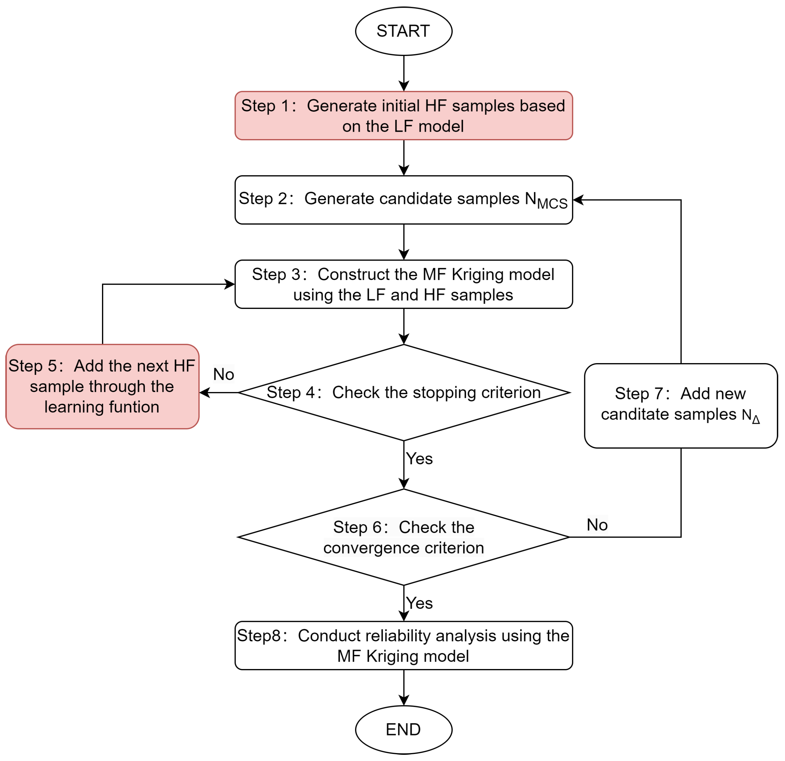
Characterized by a two-stage active learning structure, the AHK-MCS method was put forward by Feng et al. [26]. It involves the sequential construction of the LF and HF models. The HF model’s active learning process shares similarities with the LF model’s, except for employing a hierarchical Kriging model in its development. Notably, this method adopts an experimental design approach based on the LF model. Also integrated is the ESC stopping criterion [34]. Figure 2 presents the active learning process for the HF model in the second stage.

3. Comparative Results of Different MF Kriging Models

In this section, five numerical examples are employed to compare the performance of different MF Kriging models in two reliability analysis frameworks. The hierarchical Kriging model, dis-Kriging model, and Co-Kriging model are employed in the frameworks of the AHK-MCS and AMK-MCS+AEFF methods. This work thus sets out to compare six different methods. To provide a concise representation of the six methods, they are designated as AHK-MCS, ADK-MCS, ACK-MCS, AHK-MCS+AEFF, ADK-MCS+AEFF, and ACK-MCS+AEFF. The second letter of the six methods is congruent with the first letter of the MF Kriging model. The initial number of the candidate samples for the six methods is ${10}^5$. The number of initial HF samples for the six methods is five. The stopping threshold can be taken as the percentage of wrong sign estimations of the limit state function. An excessive threshold value may result in incorrect failure probability estimation [34]. In this study, the stopping threshold is set to $[0.01,0.02,0.03]$ to evaluate the performance of different MF Kriging models under varying threshold conditions [25]. If a method requires more than 100 HF samples while still failing to meet the stopping threshold, it is deemed to have failed the reliability analysis. All MF surrogate models are calculated 30 times to assess the stability of failure probability estimation.

3.1. Multimodal Function

The first example involves a two-dimensional, highly nonlinear function. Referenced from [15,35], the limit state function is expressed as

$$\begin{array}{cc}\hfill & \begin{array}{cc}\hfill G_{\mathrm{h}}\left(\mathbf{x}\right)=& 2-{\displaystyle \frac{\left(x_1^2+4\right)\left(x_2-1\right)}{20}}-sin\left({\displaystyle \frac{5x_1}{2}}\right)\hfill \\ \hfill G_{\mathrm{l}}\left(\mathbf{x}\right)=& 2-{\displaystyle \frac{\left(x_1^2+4\right)\left(x_2-1\right)}{20}}-sin\left({\displaystyle \frac{5x_1}{2}}\right)-sin\left({\displaystyle \frac{5}{22}}\left(x_1+{\displaystyle \frac{x_2}{2}}\right)+{\displaystyle \frac{5}{4}}\right)\hfill \end{array}\hfill \end{array}$$

(11)

where the parameters of the normally distributed $\mathbf{x}$ take a mean of [1.5, 2.5] and a variance of [1, 1]. The multimodal function has a cost ratio $c\left(\mathrm{h}\right)/c\left(\mathrm{l}\right)$ of 5.

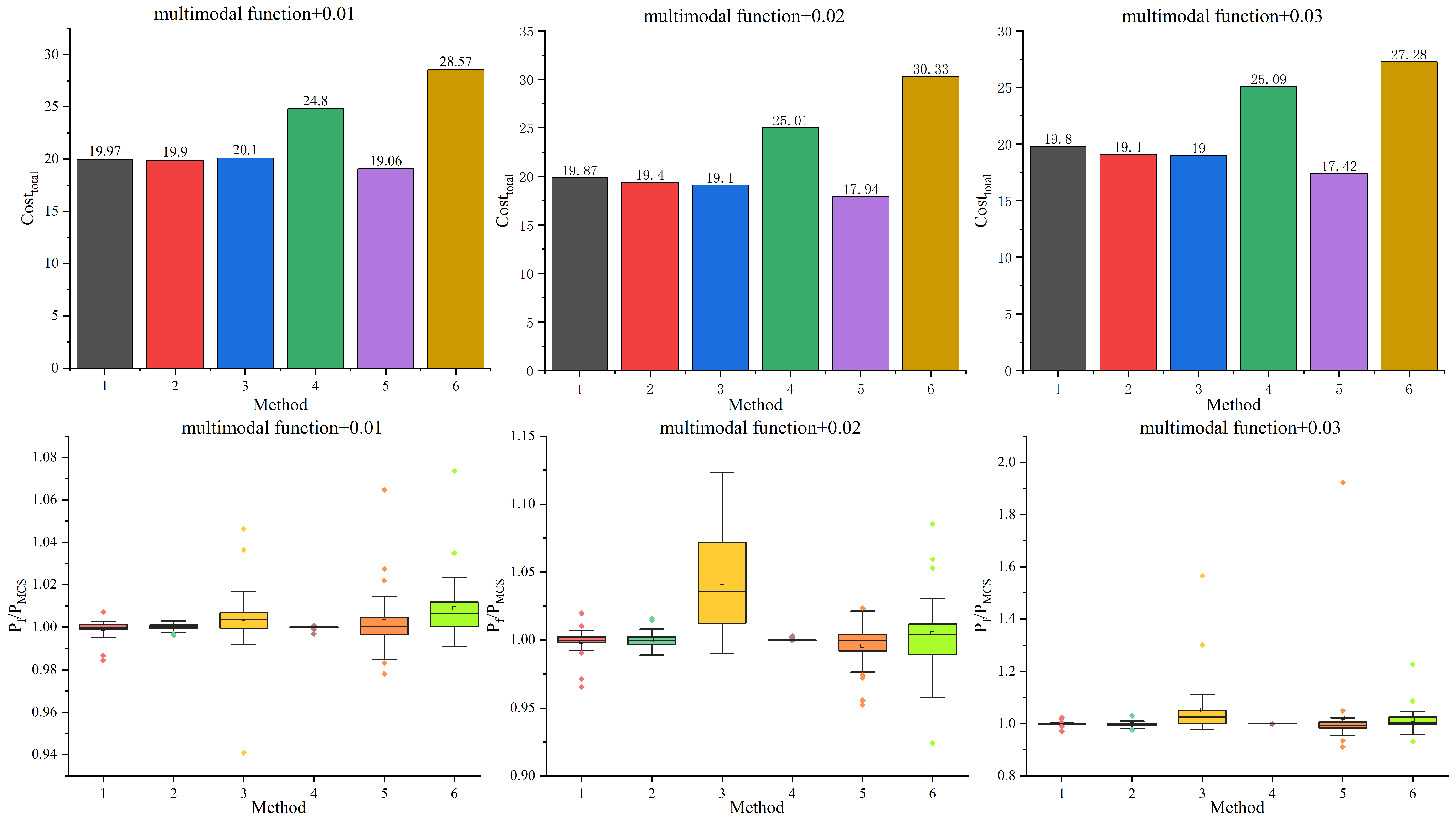
The comparative results are presented in

Table 1. Results of the multimodal function with different MF Kriging models.

Methods	Stopping Threshold	${\mathbf{N}}_{\mathbf{hf}}$	${\mathbf{N}}_{\mathbf{lf}}$	${\mathbf{Cost}}_{\mathbf{total}}$	${\mathbf{P}}_{\mathbf{f}}$ (×10−2)	Cov (%)	${\mathit{\sigma }}_{{\mathbf{P}}_{\mathbf{f}}/{\mathbf{P}}_{\mathbf{MCS}}}$
MCS	/	${10}^5$	/	${10}^5$	3.13	1.76	/
AHK-MCS	0.01	8.17	59.00	19.97	3.13	1.76	0.00431
	0.02	8.07	59.00	19.87	3.13	1.76	0.00976
	0.03	8.00	59.00	19.80	3.13	1.76	0.00825
ADK-MCS	0.01	8.10	59.00	19.90	3.13	1.76	0.00153
	0.02	7.60	59.00	19.40	3.13	1.76	0.00586
	0.03	7.30	59.00	19.10	3.13	1.76	0.00985
ACK-MCS	0.01	8.30	59.00	20.10	3.14	1.76	0.0163
	0.02	7.30	59.00	19.10	3.26	1.72	0.0396
	0.03	7.20	59.00	19.00	3.30	1.72	0.114
AHK-MCS+AEFF	0.01	14.07	53.67	24.80	3.14	1.76	0.000639
	0.02	14.03	54.90	25.01	3.13	1.76	0.000546
	0.03	14.03	55.30	25.09	3.14	1.76	0.000346
ADK-MCS+AEFF	0.01	9.47	48.00	19.06	3.14	1.76	0.0154
	0.02	8.67	46.37	17.94	3.12	1.76	0.0185
	0.03	8.33	45.43	17.42	3.20	1.75	0.172
ACK-MCS+AEFF	0.01	21.57	35.03	28.57	3.16	1.75	0.0153
	0.02	23.53	33.97	30.33	3.15	1.75	0.0296
	0.03	20.87	32.07	27.28	3.20	1.74	0.0488

. The $N_{\mathrm{hf}}$ is the number of HF samples and the $N_{\mathrm{lf}}$ is the number of LF samples. The $Cos{t}_{\mathrm{total}}$ is the total cost which equals $N_{\mathrm{hf}}+N_{\mathrm{lf}}\times c\left(\mathrm{l}\right)/c\left(\mathrm{h}\right)$. The $P_{\mathrm{f}}$ is the failure probability. In this work, ${\sigma }_{{\mathrm{P}}_{\mathrm{f}}/{\mathrm{P}}_{\mathrm{MCS}}}$ is employed to denote the standard deviation of $P_{\mathrm{f}}/P_{\mathrm{MCS}}$, with ${\sigma }_{{\mathrm{P}}_{\mathrm{f}}/{\mathrm{P}}_{\mathrm{MCS}}}$ being utilised to ascertain the stability of the MF Kriging models in predicting failure probability. A smaller ${\sigma }_{{\mathrm{P}}_{\mathrm{f}}/{\mathrm{P}}_{\mathrm{MCS}}}$ value indicates that the estimated failure probability is closer to the real failure probability. In other words, the MF Kriging model can predict the failure probability more stably. Furthermore, this paper presents the distribution of $P_{\mathrm{f}}/P_{\mathrm{MCS}}$.

As demonstrated in Table 1 and Figure 3, it is evident that all methods provide an accurate estimation of the failure probability, with the exception of the ACK-MCS method when the stopping threshold is set to be 0.02 and 0.03. The two-stage methods have overall demonstrated higher efficiencies than the one-stage methods when using the same MF Kriging model. The $N_{\mathrm{hf}}$ and the ${Cost}_{\mathrm{total}}$ of the ACK-MCS+AEFF method are maximal, while its accuracy is moderate. It should be noted that the $N_{\mathrm{hf}}$ of ACK-MCS+AEFF with a stopping threshold of 0.02 is higher than that of 0.01, since a prohibitive number of HF samples is sometimes required. This also indicates that the active learning process is unstable. Despite the fact that the ${\sigma }_{{\mathrm{P}}_{\mathrm{f}}/{\mathrm{P}}_{\mathrm{MCS}}}$ of the AHK-MCS+AEFF method is minimal, the ${Cost}_{\mathrm{total}}$ is excessive, thereby resulting in a low level of efficiency. Overall, the dis-Kriging and hierarchical Kriging models perform well in both one-stage and two-stage frameworks.

3.2. Four-Boundary Series System

The second example involves a two-dimensional, four-boundary series system. Referenced from [14,25], the limit state function is expressed as

$$\begin{array}{cc}\hfill & \begin{array}{c}\hfill G_{\mathrm{h}}\left(\mathbf{x}\right)=min\left\{\begin{array}{c}3+0.1{\left(x_1-x_2\right)}^2-\left(x_1+x_2\right)/\sqrt{2}\\ 3+0.1{\left(x_1-x_2\right)}^2+\left(x_1+x_2\right)/\sqrt{2}\\ \left(x_1-x_2\right)+7/\sqrt{2}\\ \left(x_2-x_1\right)+7/\sqrt{2}\end{array}\right.\\ \hfill G_{\mathrm{l}}\left(\mathbf{x}\right)=min\left\{\begin{array}{c}3+0.1{\left(x_1-x_2\right)}^2-\left(x_1+x_2\right)/\sqrt{2}\\ 3+0.1{\left(x_1-x_2\right)}^2+\left(x_1+x_2\right)/\sqrt{2}\\ \left(x_1-0.9x_2\right)+7/\sqrt{2}\\ \left(x_2-0.9x_1\right)+7/\sqrt{2}\end{array}\right.\end{array}\hfill \end{array}$$

(12)

where $x_1$ and $x_2$ follow a standard normal distribution. The four-boundary series system has a cost ratio $c\left(\mathrm{h}\right)/c\left(\mathrm{l}\right)$ of 5.

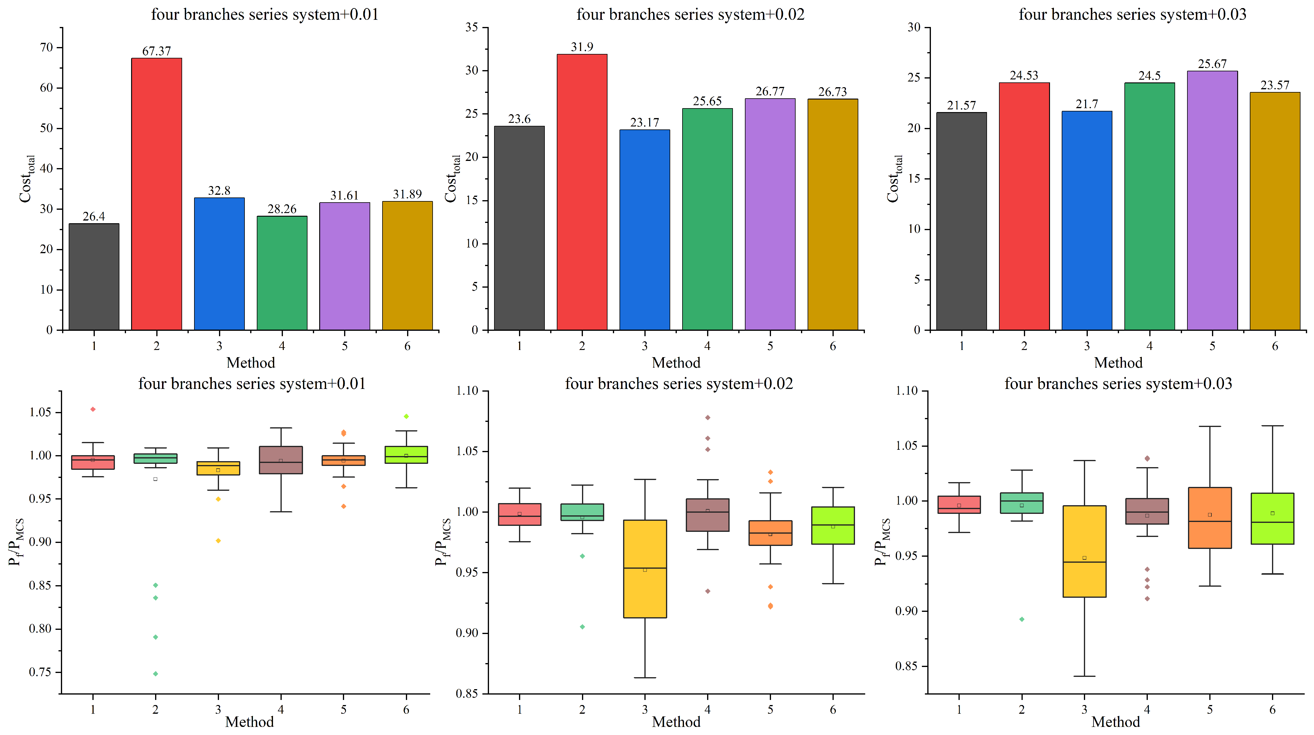
For the four-boundary series system, the results obtained with different MF Kriging models are reported in

Table 2. Results of the four-boundary series system with different MF Kriging models.

Methods	Stopping Threshold	${\mathbf{N}}_{\mathbf{hf}}$	${\mathbf{N}}_{\mathbf{lf}}$	${\mathbf{Cost}}_{\mathbf{total}}$	${\mathbf{P}}_{\mathbf{f}}$ (×10−2)	Cov (%)	${\mathit{\sigma }}_{{\mathbf{P}}_{\mathbf{f}}/{\mathbf{P}}_{\mathbf{MCS}}}$
MCS	/	$2\times {10}^5$	/	$2\times {10}^5$	2.23	4.73	/
AHK-MCS	0.01	15.00	57.00	26.40	2.22	4.74	0.0145
	0.02	12.20	57.00	23.60	2.23	4.73	0.0122
	0.03	10.17	57.00	21.57	2.23	4.74	0.0114
ADK-MCS	0.01	55.97	57.00	67.37	2.18	4.84	0.0683
	0.02	20.50	57.00	31.90	2.23	4.73	0.0210
	0.03	13.13	57.00	24.53	2.23	4.73	0.0225
ACK-MCS	0.01	21.40	57.00	32.80	2.20	4.63	0.0199
	0.02	11.77	57.00	23.17	2.13	4.49	0.0455
	0.03	10.30	57.00	21.70	2.12	4.49	0.0549
AHK-MCS+AEFF	0.01	17.00	56.30	28.26	2.21	4.72	0.0217
	0.02	15.17	52.43	25.65	2.22	4.74	0.0281
	0.03	14.33	50.83	24.50	2.20	4.77	0.0301
ADK-MCS+AEFF	0.01	29.80	65.23	31.61	2.20	4.76	0.0163
	0.02	14.97	59.00	26.77	2.16	4.75	0.0254
	0.03	13.83	59.16	25.67	2.20	4.65	0.0365
ACK-MCS+AEFF	0.01	19.53	61.77	31.89	2.23	4.70	0.0165
	0.02	15.47	56.30	26.73	2.18	4.73	0.0199
	0.03	13.10	52.37	23.57	2.23	4.74	0.0393

and Figure 4. The two-stage method demonstrates a superior efficiency and stability compared with the one-stage approach when employing the hierarchical Kriging model. The dispersion of the failure probability of the ACK-MCS method remains high at stopping thresholds of 0.02 and 0.03, while $N_{\mathrm{hf}}$ shows a substantial increase at 0.01, demonstrating that the ACK-MCS method exhibits excessive sensitivity to the stopping threshold. The $N_{\mathrm{hf}}$ and ${\sigma }_{{\mathrm{P}}_{\mathrm{f}}/{\mathrm{P}}_{\mathrm{MCS}}}$ of the ADK-MCS method when the stopping threshold is set to 0.01 are excessively high, indicating that an excessively low stopping threshold is unnecessary. The results of the four-boundary series system show that both the Co-Kriging and dis-Kriging models perform poorly in the two-stage framework, and they offer no significant advantage over hierarchical Kriging in the one-stage framework. The hierarchical Kriging method demonstrates a superior efficiency and stability for this example.

3.3. Four-Dimensional Park Function

The third example involves a four-dimensional park function, a test case for high-dimensional problems [36]. The limit state function of the four-dimensional park function is expressed by

$$\begin{array}{cc}\hfill & \begin{array}{cc}\hfill G_{\mathrm{h}}\left(\mathbf{x}\right)=& {\displaystyle \frac{x_1}{2}}\left(\sqrt{\left(\left(x_2+x_3^2\right){\displaystyle \frac{x_4}{x_1^2}}\right)}+1\right)+\left(x_1+3x_4\right)\exp \left(\sin \left(x_3\right)+1\right)-2\hfill \\ \hfill G_{\mathrm{l}}\left(\mathbf{x}\right)=& \left({\displaystyle \frac{\sin \left(x_1\right)}{10}}+1\right)G_{\mathrm{h}}\left(\mathbf{x}\right)+x_2^2+x_3^2-2x_1+0.5\hfill \end{array}\hfill \end{array}$$

(13)

where the variables are uniformly distributed in $[0,1]$. The four-dimensional park function has a cost ratio $c\left(\mathrm{h}\right)/c\left(\mathrm{l}\right)$ of 10.

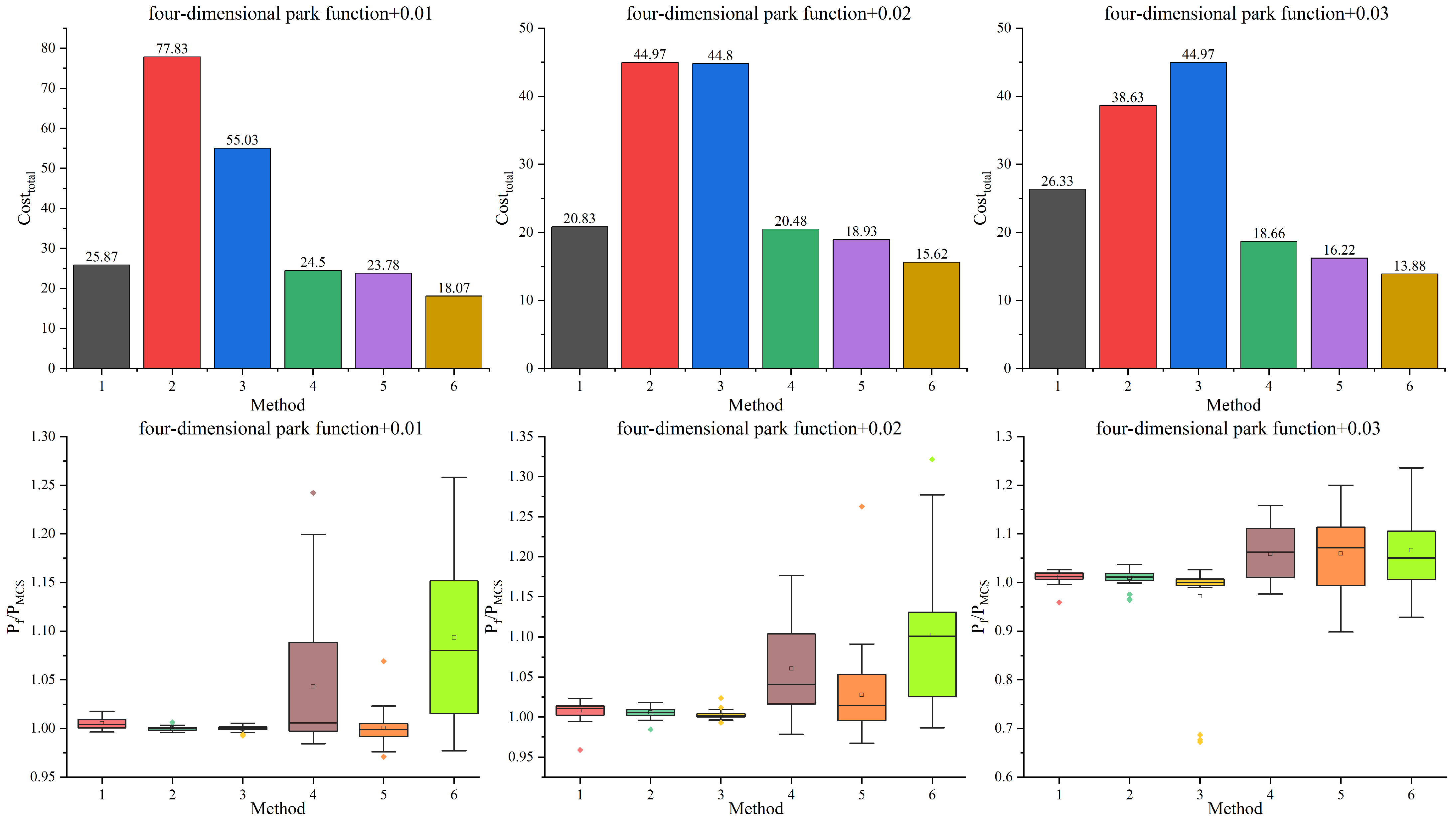
For the four-dimensional park function, the results obtained with different MF Kriging models are reported in

Table 3. Results of the four-dimensional park function with different MF Kriging models.

Methods	Stopping Threshold	${\mathbf{N}}_{\mathbf{hf}}$	${\mathbf{N}}_{\mathbf{lf}}$	${\mathbf{Cost}}_{\mathbf{total}}$	${\mathbf{P}}_{\mathbf{f}}$ (×10−2)	Cov (%)	${\mathit{\sigma }}_{{\mathbf{P}}_{\mathbf{f}}/{\mathbf{P}}_{\mathbf{MCS}}}$
MCS	/	$1\times {10}^5$	/	$1\times {10}^5$	3.85	1.58	/
AHK-MCS	0.01	18.77	71.00	25.87	3.86	1.58	0.0061
	0.02	13.73	71.00	20.83	3.88	1.57	0.0119
	0.03	12.13	71.00	19.23	3.89	1.57	0.0125
ADK-MCS	0.01	70.73	71.00	77.83	3.85	1.58	0.0022
	0.02	37.87	71.00	44.97	3.87	1.58	0.0067
	0.03	24.43	71.00	31.53	3.88	1.58	0.0167
ACK-MCS	0.01	47.93	71.00	55.03	3.84	1.58	0.0029
	0.02	37.70	71.00	44.80	3.86	1.58	0.0055
	0.03	30.77	71.00	37.87	3.73	1.61	0.0997
AHK-MCS+AEFF	0.01	19.07	54.37	24.50	4.00	1.55	0.0718
	0.02	15.33	51.47	20.48	4.07	1.54	0.0558
	0.03	14.40	42.60	18.66	4.06	1.54	0.0521
ADK-MCS+AEFF	0.01	18.77	50.13	23.78	3.84	1.58	0.0170
	0.02	14.60	43.30	18.93	3.95	1.56	0.0550
	0.03	12.30	39.17	16.22	4.08	1.54	0.0800
ACK-MCS+AEFF	0.01	12.93	51.40	18.07	4.20	1.51	0.0833
	0.02	11.17	44.50	15.62	4.25	1.51	0.0939
	0.03	9.73	41.43	13.88	4.09	1.53	0.0805

and Figure 5. In terms of precision, the two-stage methods demonstrate a superior performance compared with the one-stage methods. The stability of the one-stage methods is also unsatisfactory. Notably, the two-stage methods utilise 71 LF samples, whereas the one-stage methods employ fewer than 55 LF samples. An insufficient number of LF samples might account for the inferior performance of the one-stage methods, particularly for the hierarchical Kriging model [26]. The ADK-MCS and ACK-MCS methods show a significant increase in ${\sigma }_{{\mathrm{P}}_{\mathrm{f}}/{\mathrm{P}}_{\mathrm{MCS}}}$ when the stopping threshold is set to 0.03. The hierarchical Kriging model outperforms the other MF Kriging models within the two-stage framework by requiring the fewest HF samples to correctly construct the HF model.

3.4. Nonlinear Oscillator System

The fourth example considers a six-dimensional nonlinear oscillator system [25,37], depicted in Figure 6, whose limit state function is given by

$$\begin{array}{cc}\hfill & \begin{array}{cc}\hfill & G_{\mathrm{h}}\left(c_1,c_2,m,r,t_1,F_1\right)=3r-\left|{\displaystyle \frac{2F_1}{m{\omega }_0^2}}sin\left({\displaystyle \frac{{\omega }_0{t}_1}{2}}\right)\right|\hfill \\ \hfill & G_{\mathrm{l}}\left(c_1,c_2,m,r,t_1,F_1\right)=3r-\left|{\displaystyle \frac{2F_1}{m{\omega }_0^2}}sin\left({\displaystyle \frac{{\omega }_0{t}_1}{2}}-0.1\right)\right|\hfill \end{array}\hfill \end{array}$$

(14)

where ${\omega }_0=\sqrt{\left(c_1+c_1\right)/m}$. The statistics of the variables are summarized in

Table 4. Statistics of the variables of the nonlinear oscillator system.

Variables	Mean	Standard Deviation	Distribution
$m\left(\mathrm{kg}\right)$	1	0.05	Normal
$c_1(\mathrm{N}/\mathrm{mm})$	1	0.1	Normal
$c_2(\mathrm{N}/\mathrm{mm})$	0.1	0.01	Normal
$r\left(\mathrm{mm}\right)$	0.5	0.05	Normal
$f_1\left(\mathrm{N}\right)$	1	0.1	Normal
$t_1\left(\mathrm{s}\right)$	1	0.1	Normal

. The nonlinear oscillator system has a cost ratio $c\left(\mathrm{h}\right)/c\left(\mathrm{l}\right)$ of 10.

Table 5. Results of the nonlinear oscillator system with different MF Kriging models.

Methods	Stopping Threshold	${\mathbf{N}}_{\mathbf{hf}}$	${\mathbf{N}}_{\mathbf{lf}}$	${\mathbf{Cost}}_{\mathbf{total}}$	${\mathbf{P}}_{\mathbf{f}}$ (×10−2)	Cov (%)	${\mathit{\sigma }}_{{\mathbf{P}}_{\mathbf{f}}/{\mathbf{P}}_{\mathbf{MCS}}}$
MCS	/	$2\times {10}^5$	/	$2\times {10}^5$	2.42	4.54	/
AHK-MCS	0.01	47.33	47.00	52.03	2.43	4.54	0.00562
	0.02	17.07	47.00	21.77	2.43	4.43	0.0193
	0.03	11.07	47.00	15.77	2.38	4.58	0.0416
ADK-MCS	0.01	failed	/	/	/	/	/
	0.02	68.03	47.00	72.73	2.43	4.54	0.00445
	0.03	26.50	47.00	31.20	2.43	4.54	0.0120
ACK-MCS	0.01	82.23	47.00	86.93	2.43	4.59	0.00682
	0.02	41.90	47.00	46.60	2.43	4.54	0.0178
	0.03	33.77	47.00	38.47	2.42	4.54	0.0178
AHK-MCS+AEFF	0.01	21.03	80.17	29.05	2.44	4.53	0.0126
	0.02	16.56	71.73	23.74	2.43	4.54	0.0359
	0.03	14.97	69.87	21.95	2.49	4.48	0.0414
ADK-MCS+AEFF	0.01	29.80	94.53	39.25	2.39	4.57	0.0110
	0.02	20.17	83.63	28.53	2.47	4.50	0.0168
	0.03	15.40	71.93	22.59	2.42	4.54	0.0282
ACK-MCS+AEFF	0.01	13.37	88.73	22.24	2.41	4.56	0.0152
	0.02	9.83	75.57	17.39	2.52	4.46	0.0456
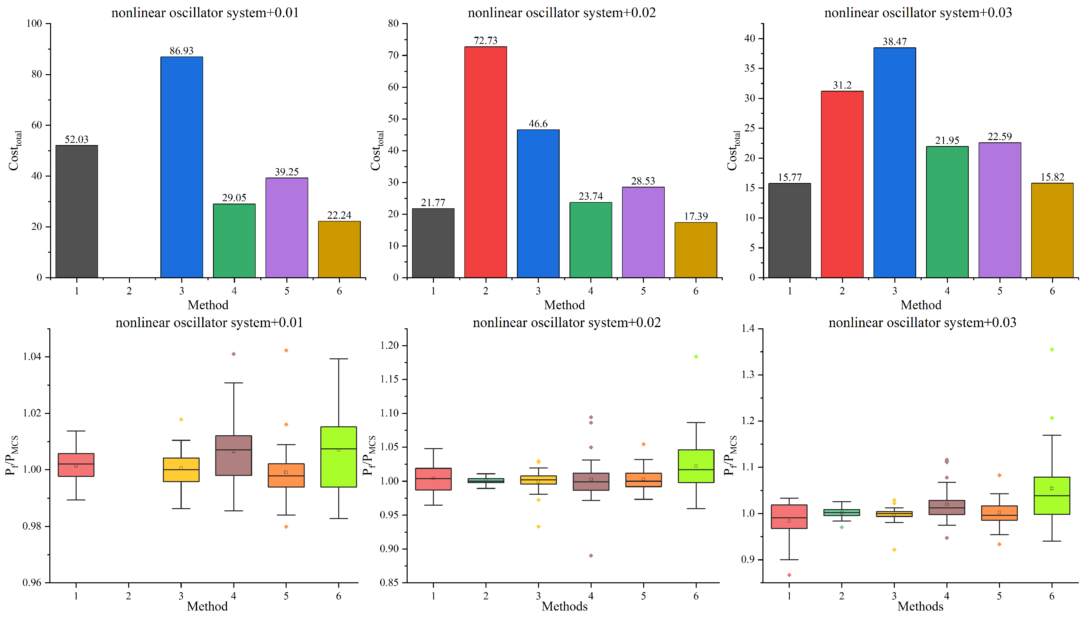
	0.03	8.87	69.53	15.82	2.56	4.43	0.0872

and Figure 7 show the results of the nonlinear oscillator system with different MF Kriging models. With the stopping threshold configured at 0.01, the AHK-MCS and ACK-MCS methods demonstrate excessively high $N_{\mathrm{hf}}$ values, although they maintain low ${\sigma }_{{\mathrm{P}}_{\mathrm{f}}/{\mathrm{P}}_{\mathrm{MCS}}}$ values. The ADK-MCS method fails to reach the stopping threshold when it is set to 0.01. This indicates that employing a stringent stopping threshold may be unnecessary for the nonlinear oscillator system. The ADK-MCS method underperforms among the one-stage methods and the ${Cost}_{\mathrm{total}}$ of the ADK-MCS+AEFF method is the highest among the two-stage framework methods, which indicates that the dis-Kriging method has limited capabilities in handling complex problems. Co-Kriging yields a relatively low ${Cost}_{\mathrm{total}}$ in the one-stage framework, whereas its performance deteriorates in the two-stage framework, resulting in a substantially higher cost. It is evident that the ${Cost}_{\mathrm{total}}$ of the ACK-MCS+AEFF method is less in the one-stage methods, whilst the ${Cost}_{\mathrm{total}}$ of the ACK-MCS method is more in the two-stage methods. Moreover, the stability of the ACK-MCS+AEFF method remains unsatisfactory. It should be noted that when applying the ACK-MCS+AEFF method to the four-dimensional park function and the nonlinear oscillator system, premature reaching of the stopping threshold frequently occurs, consequently leading to inaccurate failure probability estimation. The hierarchical Kriging model performs well in both one-stage and two-stage frameworks.

3.5. Vehicle Side Impact Problem

The fifth example involves a seven-dimensional vehicle side impact problem. Referenced from [24,38], the problem is expressed as

$$\begin{array}{cc}\hfill & \begin{array}{cc}\hfill G_{\mathrm{hf}}\left(\mathbf{x}\right)=& 0.489x_1{x}_4+0.843x_2{x}_3-0.0432x_5{x}_6+0.0556x_5{x}_7+0.00078x_7^2-0.75\hfill \\ \hfill G_{\mathrm{lf}}\left(\mathbf{x}\right)=& G_{\mathrm{hf}}\left(\mathbf{x}\right)-{\displaystyle \frac{1}{10}}\left(\right(0.489\left(x_1-0.1\right)\left(x_4-0.1\right)+0.843\left(x_2-0.1\right)\left(x_3-0.1\right)\hfill \\ \hfill & +0.0432\left(x_5-0.1\right)\left(x_6-0.1\right)+0.0556\left(x_5-0.1\right)\left(x_7-0.1\right)+0.00078\left(x_7-1\right))\hfill \end{array}\hfill \end{array}$$

(15)

In the vehicle side impact problem, the statistical parameters of the variables have been adjusted compared to those in [38]. This modification aims to increase the failure probability, thereby reducing the number of candidate samples required. The statistics of the variables are summarized in

Table 6. Statistics of the variables of the vehicle side impact problem.

Variables	Mean	Standard Deviation	Distribution
$x_1$	1.15	0.3	Normal
$x_2$	1.15	0.3	Normal
$x_3$	1.15	0.3	Normal
$x_4$	1.15	0.3	Normal
$x_5$	0.3	0.06	Normal
$x_6$	0	10	Normal
$x_7$	0	10	Normal

. The cost ratio $c\left(\mathrm{h}\right)/c\left(\mathrm{l}\right)$ of this problem is changed from 20 to 5 to avoid too many LF samples.

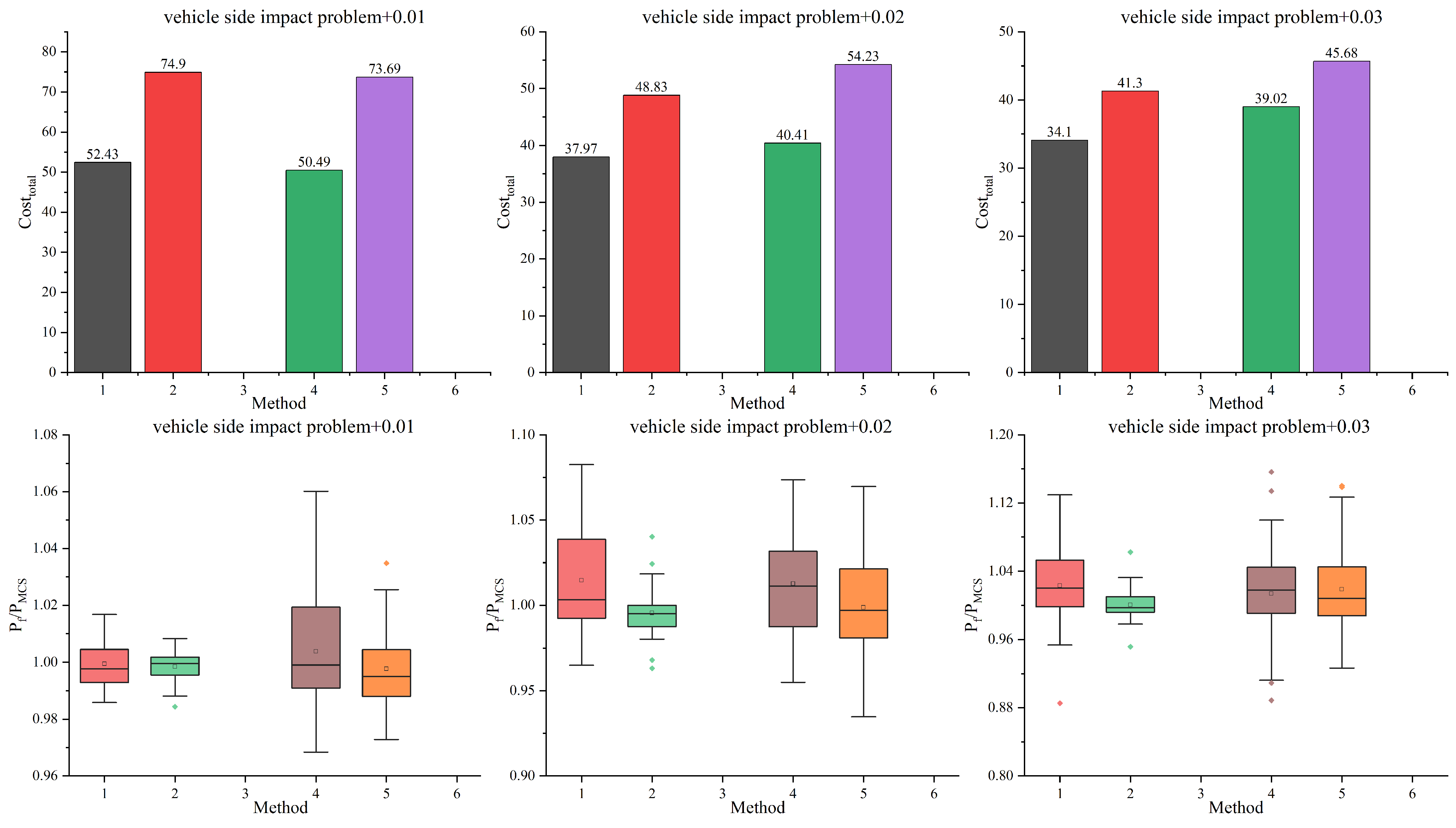
The results of the vehicle side impact problem are set out in

Table 7. Results of the vehicle side impact problem with different MF Kriging models.

Methods	Stopping Threshold	${\mathbf{N}}_{\mathbf{hf}}$	${\mathbf{N}}_{\mathbf{lf}}$	${\mathbf{Cost}}_{\mathbf{total}}$	${\mathbf{P}}_{\mathbf{f}}$ (×10−2)	Cov (%)	${\mathit{\sigma }}_{{\mathbf{P}}_{\mathbf{f}}/{\mathbf{P}}_{\mathbf{MCS}}}$
MCS	/	${10}^5$	/	${10}^5$	1.10	3.00	/
AHK-MCS	0.01	27.23	126.00	52.43	1.10	2.99	0.0081
	0.02	12.77	126.00	37.97	1.12	2.97	0.0320
	0.03	8.90	126.00	34.10	1.13	2.96	0.0502
ADK-MCS	0.01	49.70	126.00	74.90	1.10	3.00	0.0053
	0.02	23.63	126.00	48.83	1.10	3.00	0.0148
	0.03	16.10	126.00	41.30	1.10	2.99	0.0191
ACK-MCS	0.01	failed	/	/	/	/	/
	0.02	failed	/	/	/	/	/
	0.03	failed	/	/	/	/	/
AHK-MCS+AEFF	0.01	24.77	128.60	50.49	1.10	2.99	0.0196
	0.02	16.33	120.40	40.41	1.11	2.99	0.0353
	0.03	15.27	118.77	39.02	1.12	2.98	0.0613
ADK-MCS+AEFF	0.01	39.30	171.93	73.69	1.10	3.00	0.0158
	0.02	30.00	144.50	54.23	1.10	2.99	0.0318
	0.03	19.80	129.40	45.68	1.12	2.97	0.0556
ACK-MCS+AEFF	0.01	failed	/	/	/	/	/
	0.02	failed	/	/	/	/	/
	0.03	failed	/	/	/	/	/

and Figure 8. The ACK-MCS and ACK-MCS+AEFF methods are not capable of satisfying the stopping thresholds. This indicates that the Co-Kriging model performs poorly in handling complex and multivariable problems. In general, the two-stage methods demonstrate superior performances in comparison to the one-stage methods. Although the ${\sigma }_{{\mathrm{P}}_{\mathrm{f}}/{\mathrm{P}}_{\mathrm{MCS}}}$ index when using the dis-Kriging model is lower than when using the hierarchical Kriging model, the ${Cost}_{\mathrm{total}}$ and the $N_{\mathrm{hf}}$ for the dis-Kriging model are significantly greater than those for the hierarchical Kriging model. This indicates that the dis-Kriging model is deficient in its ability to address complex problems. The hierarchical Kriging model has been shown to exhibit a superior performance in both one-stage and two-stage frameworks when compared with the dis-Kriging model.

4. Discussion

In this work, three MF Kriging models are compared in two types of MF active learning frameworks, i.e., six active learning MF methods are employed. The performances of the hierarchical Kriging model, the dis-Kriging model, and the Co-Kriging model are explored through five numerical examples. In general, the three MF Kriging models have been demonstrated to possess the capacity to predict failure probability except for the vehicle side impact problem. It has been shown that two-stage methods overall outperform one-stage methods for the estimation of failure probability, both in terms of efficiency and stability. The primary rationale for this phenomenon lies in the two-stage methods’ full utilization of the LF model to reduce the required number of HF samples [26]. The influence of the stopping threshold is also studied in this work. As the stopping threshold decreases, the number of required HF samples and the stability of failure probability generally increase. Nevertheless, an excessively low stopping threshold is not necessary. In some cases, setting an excessively low stopping threshold may prevent the threshold from being met. It should be noted that extreme values of $P_{\mathrm{f}}/P_{\mathrm{MCS}}$ appear rarely. These cases mainly occur when thresholds are set at 0.01 or 0.03, indicating overfitting or underfitting. This highlights the need for a more robust stopping criterion.

To summarise the results of the five numerical examples, it can be concluded that the hierarchical Kriging model performs relatively well in both the one-stage and two-stage frameworks. The advantages of the hierarchical Kriging model in the two-stage framework are more readily apparent because the constructed high-precision LF model is used to predict the basis function of the observed samples. Consequently, the trend of the LF function is effectively mapped to the sampled HF data, thereby yielding a more accurate surrogate model for the HF function. Furthermore, the hierarchical Kriging model demonstrates a superior performance in estimating the MSE compared with both the dis-Kriging and Co-Kriging methods. It has been posited that the hierarchical Kriging model is an efficient, accurate, and robust model [31]. The dis-Kriging model demonstrates a strong performance in the multimodal function and four-boundary series system examples. Nevertheless, its efficacy is less pronounced in the four-dimensional park function, nonlinear oscillator systems, and vehicle side impact problem. This indicates that the dis-Kriging model lacks sufficient capacity to address intricate, high-degree nonlinear problems. The dis-Kriging model is a concise form of the MF Kriging model. However, its MSE is simply the sum of the MSE of the LF Kriging model and the discrepancy Kriging model, which fails to fully capture the uncertainty of the predicted values. The Co-Kriging model demonstrates an unstable performance when handling five numerical examples, especially for multi-dimensional nonlinear problems. Furthermore, the ACK-MCS and ACK-MCS+AEFF methods do not reach the stopping threshold in the vehicle side impact problem. Studies of the five examples demonstrate the limited robustness of the Co-Kriging model. A plausible explanation for this phenomenon is that the Co-Kriging model incorporates a significantly larger correlation matrix than both hierarchical Kriging and dis-Kriging. As the dimensionality of the problem increases, the complexity of the correlation matrix grows proportionally. This poses greater challenges to obtain the model parameters through optimization methods, consequently leading to diminished robustness.

Based on the results of the five examples, it is suggested that the hierarchical Kriging model could be employed for MF reliability analysis. The dis-Kriging model is recommended for simple situations. Considering that the robustness of the Co-Kriging model is not satisfactory, it is not currently recommended to use the Co-Kriging model for MF reliability analysis. It should be pointed out that the Co-Kriging model utilized is derived from the ooDACE toolbox [33]. It is reasonable to expect that improved optimization methods for the Co-Kriging model could enhance its robustness in MF active learning methods.

It is important to note that the examples employed in this study are primarily numerical simulations, although the last two examples actually originate from engineering backgrounds. However, real-world scenarios typically involve greater uncertainty and noise within samples. To achieve a more comprehensive evaluation of the performance of different Kriging-based metamodels, it is imperative to incorporate authentic engineering problems into subsequent comparative analyses. It should be noted that several new Kriging-based models have also been proposed [9,39]. It is suggested to conduct further comparative research on a broader range of Kriging models.

5. Conclusions

In this study, the performance of three MF Kriging models is compared in two active learning frameworks. The five examples demonstrate the following: the hierarchical Kriging model performs relatively well in both the one-stage and two-stage frameworks; the dis-Kriging model is not adequately equipped to address complex, highly nonlinear problems; and the Co-Kriging model is limited in terms of robustness, though it performs well in some instances. Based on the results from the five examples, guidance for selecting appropriate MF Kriging models is proposed. These findings will inform the development of future MF active learning methods.

References

1. Song, C.; Kawai, R. Monte Carlo and variance reduction methods for structural reliability analysis: A comprehensive review. Probabilist. Eng. Mech. 2023, 73, 103479. [Google Scholar] [CrossRef]
2. Liu, J.; Shi, Y.; Ding, C.; Beer, M. Hybrid uncertainty propagation based on multi-fidelity surrogate model. Comput. Struct. 2024, 293, 107267. [Google Scholar] [CrossRef]
3. Teixeira, R.; Nogal, M.; O’Connor, A. Adaptive approaches in metamodel-based reliability analysis: A review. Struct. Saf. 2021, 89, 102019. [Google Scholar] [CrossRef]
4. Moustapha, M.; Marelli, S.; Sudret, B. Active learning for structural reliability: Survey, general framework and benchmark. Struct. Saf. 2022, 96, 102174. [Google Scholar] [CrossRef]
5. Lu, N.; Li, Y.F.; Mi, J.; Huang, H.Z. AMFGP: An active learning reliability analysis method based on multi-fidelity Gaussian process surrogate model. Reliab. Eng. Syst. Saf. 2024, 246, 110020. [Google Scholar] [CrossRef]
6. Chun, J. Active Learning-Based Kriging Model with Noise Responses and Its Application to Reliability Analysis of Structures. Appl. Sci. 2024, 14, 882. [Google Scholar] [CrossRef]
7. Faravelli, L. Response-surface approach for reliability analysis. J. Eng. Mech. 1989, 115, 2763–2781. [Google Scholar] [CrossRef]
8. Krige, D.G. A statistical approach to some basic mine valuation problems on the Witwatersrand. J. South Afr. Inst. Min. Metall. 1951, 52, 119–139. [Google Scholar]
9. Schöbi, R.; Sudret, B.; Wiart, J. Polynomial-Chaos-Based Kriging. Int. J. Uncertain. Quantif. 2015, 5, 171–193. [Google Scholar] [CrossRef]
10. Park, J.; Sandberg, I. Approximation and Radial-Basis-Function Networks. Neural Comput. 1993, 5, 305–316. [Google Scholar] [CrossRef]
11. Rocco, C.M.; Moreno, J.A. Fast Monte Carlo reliability evaluation using support vector machine. Reliab. Eng. Syst. Saf. 2002, 76, 237–243. [Google Scholar] [CrossRef]
12. Sobol’, I.M. Theorems and examples on high dimensional model representation. Reliab. Eng. Syst. Saf. 2003, 79, 187–193. [Google Scholar] [CrossRef]
13. Gaspar, B.; Teixeira, A.; Soares, C.G. Assessment of the efficiency of Kriging surrogate models for structural reliability analysis. Probabilist. Eng. Mech. 2014, 37, 24–34. [Google Scholar] [CrossRef]
14. Echard, B.; Gayton, N.; Lemaire, M. AK-MCS: An active learning reliability method combining Kriging and Monte Carlo Simulation. Struct. Saf. 2011, 33, 145–154. [Google Scholar] [CrossRef]
15. Bichon, B.J.; Eldred, M.S.; Swiler, L.P.; Mahadevan, S.; McFarland, J.M. Efficient Global Reliability Analysis for Nonlinear Implicit Performance Functions. AIAA J. 2008, 46, 2459–2468. [Google Scholar] [CrossRef]
16. Zhao, Z.; Xie, L.; Zhao, B.; Song, J.; Wang, L. Reliability evaluation of folding wing mechanism deployment performance based on improved active learning Kriging method. Probabilist. Eng. Mech. 2023, 74, 103547. [Google Scholar] [CrossRef]
17. Okoro, A.; Khan, F.; Ahmed, S. An Active Learning Polynomial Chaos Kriging metamodel for reliability assessment of marine structures. Ocean Eng. 2021, 235, 109399. [Google Scholar] [CrossRef]
18. Qian, H.M.; Huang, T.; Wei, J.; Huang, H.Z. Active learning strategy-based reliability assessment on the wear of spur gears. J. Mech. Sci. Technol. 2023, 37, 6467–6476. [Google Scholar] [CrossRef]
19. Allahvirdizadeh, R.; Andersson, A.; Karoumi, R. Improved dynamic design method of ballasted high-speed railway bridges using surrogate-assisted reliability-based design optimization of dependent variables. Reliab. Eng. Syst. Saf. 2023, 238, 109406. [Google Scholar] [CrossRef]
20. Toal, D.J.J. Some considerations regarding the use of multi-fidelity Kriging in the construction of surrogate models. Struct. Multidiscip. Optim. 2014, 51, 1223–1245. [Google Scholar] [CrossRef]
21. Forrester, A.I.; Sóbester, A.; Keane, A.J. Multi-fidelity optimization via surrogate modelling. Proc. R. Soc. A Math. Phys. Eng. Sci. 2007, 463, 3251–3269. [Google Scholar] [CrossRef]
22. Lin, W.; Zou, M.; Zhao, M.; Chang, J.; Xie, X. Multi-Fidelity Machine Learning for Identifying Thermal Insulation Integrity of Liquefied Natural Gas Storage Tanks. Appl. Sci. 2024, 15, 33. [Google Scholar] [CrossRef]
23. Slotnick, J.P.; Khodadoust, A.; Alonso, J.J.; Darmofal, D.L.; Gropp, W.D.; Lurie, E.A.; Mavriplis, D.J.; Venkatakrishnan, V. Enabling the environmentally clean air transportation of the future: A vision of computational fluid dynamics in 2030. Philos. Trans. R. Soc. Math. Phys. Eng. Sci. 2014, 372, 20130317. [Google Scholar] [CrossRef]
24. Yi, J.; Wu, F.; Zhou, Q.; Cheng, Y.; Ling, H.; Liu, J. An active-learning method based on multi-fidelity Kriging model for structural reliability analysis. Struct. Multidiscip. Optim. 2020, 63, 173–195. [Google Scholar] [CrossRef]
25. Yi, J.; Cheng, Y.; Liu, J. A novel fidelity selection strategy-guided multifidelity kriging algorithm for structural reliability analysis. Reliab. Eng. Syst. Saf. 2022, 219, 108247. [Google Scholar] [CrossRef]
26. Feng, S.; Wang, L.; Dong, H.; Li, Y.; Wan, Z.; Guedes Soares, C. An active-learning method based on hierarchical kriging model for multi-fidelity reliability analysis. Reliab. Eng. Syst. Saf. 2026, 266, 111759. [Google Scholar] [CrossRef]
27. Che, Y.; Ma, Y.; Chen, H.; Ma, Y. Multi-fidelity kriging structural reliability analysis with the fusion of non-hierarchical low-fidelity models. Reliab. Eng. Syst. Saf. 2026, 266, 111662. [Google Scholar] [CrossRef]
28. Lima, J.P.; Evangelista, F.; Guedes Soares, C. Bi-fidelity Kriging model for reliability analysis of the ultimate strength of stiffened panels. Mar. Struct. 2023, 91, 103464. [Google Scholar] [CrossRef]
29. Dong, X.; Yang, T.; Gao, Y.; Deng, W.; Liu, Y.; Niu, P.; Jiao, S.; Zhao, Y. Conditional random field approach combining FFT filtering and Co-kriging for reliability assessment of slopes. Appl. Sci. 2025, 15, 8858. [Google Scholar] [CrossRef]
30. Lophaven, S.N.; Nielsen, H.B.; Sondergaard, J.; Dace, A. DACE: A Matlab Kriging Toolbox; Technical Report No. IMM-TR-2002-12; Technical University of Denmark: Kongens Lyngby, Denmark, 2002. [Google Scholar]
31. Han, Z.H.; Görtz, S. Hierarchical Kriging Model for Variable-Fidelity Surrogate Modeling. AIAA J. 2012, 50, 1885–1896. [Google Scholar] [CrossRef]
32. Kennedy, M.; O’Hagan, A. Predicting the output from a complex computer code when fast approximations are available. Biometrika 2000, 87, 1–13. [Google Scholar] [CrossRef]
33. Ulaganathan, S.; Couckuyt, I.; Deschrijver, D.; Laermans, E.; Dhaene, T. A Matlab Toolbox for Kriging Metamodelling. Procedia Comput. Sci. 2015, 51, 2708–2713. [Google Scholar] [CrossRef]
34. Wang, Z.; Shafieezadeh, A. ESC: An efficient error-based stopping criterion for kriging-based reliability analysis methods. Struct. Multidiscip. Optim. 2018, 59, 1621–1637. [Google Scholar] [CrossRef]
35. Chaudhuri, A.; Marques, A.N.; Willcox, K. mfEGRA: Multifidelity efficient global reliability analysis through active learning for failure boundary location. Struct. Multidiscip. Optim. 2021, 64, 797–811. [Google Scholar] [CrossRef]
36. Palar, P.S.; Tsuchiya, T.; Parks, G.T. Multi-fidelity non-intrusive polynomial chaos based on regression. Comput. Methods Appl. Mech. Eng. 2016, 305, 579–606. [Google Scholar] [CrossRef]
37. Rajashekhar, M.R.; Ellingwood, B.R. A new look at the response surface approach for reliability analysis. Struct. Saf. 1993, 12, 205–220. [Google Scholar] [CrossRef]
38. Youn, B.D.; Choi, K.K.; Yang, R.J.; Gu, L. Reliability-based design optimization for crashworthiness of vehicle side impact. Struct. Multidiscip. Optim. 2004, 26, 272–283. [Google Scholar] [CrossRef]
39. Zhang, W.; Wang, Z.; Wang, H.; Li, Z.; Wang, Y.; Zhao, Z. AEK-MFIS: An adaptive ensemble of Kriging models based on multi-fidelity simulations and importance sampling for small failure probabilities. Comput. Methods Appl. Mech. Eng. 2025, 441, 117952. [Google Scholar] [CrossRef]
Figure 1. Flowchart of the AMK-MCS+AEFF method.
Applsci 15 12607 g001
Figure 2. Flowchart of the active learning process of the HF model within AHK-MCS method.
Applsci 15 12607 g002
Figure 3. C o s t total and P f / P MCS of the multimodal function with different MF Kriging models (1: AHK-MCS, 2: ADK-MCS, 3: ACK-MCS, 4: AHK-MCS+AEFF, 5: ADK-MCS+AEFF, 6: ACK-MCS+AEFF).
Applsci 15 12607 g003
Figure 4. C o s t total and P f / P MCS of the four-boundary series system with different MF Kriging models (1: AHK-MCS, 2: ADK-MCS, 3: ACK-MCS, 4: AHK-MCS+AEFF, 5: ADK-MCS+AEFF, 6: ACK-MCS+AEFF).
Applsci 15 12607 g004
Figure 5. C o s t total and P f / P MCS of the four-dimensional park function with different MF Kriging models (1: AHK-MCS, 2: ADK-MCS, 3: ACK-MCS, 4: AHK-MCS+AEFF, 5: ADK-MCS+AEFF, 6: ACK-MCS+AEFF).
Applsci 15 12607 g005
Figure 6. Schematic diagram of the nonlinear oscillator system.
Applsci 15 12607 g006
Figure 7. C o s t total and P f / P MCS of the nonlinear oscillator system with different MF Kriging models (1: AHK-MCS, 2: ADK-MCS, 3: ACK-MCS, 4: AHK-MCS+AEFF, 5: ADK-MCS+AEFF, 6: ACK-MCS+AEFF).
Applsci 15 12607 g007
Figure 8. C o s t total and P f / P MCS of the vehicle side impact problem with different MF Kriging models (1: AHK-MCS, 2: ADK-MCS, 3: ACK-MCS, 4: AHK-MCS+AEFF, 5: ADK-MCS+AEFF, 6: ACK-MCS+AEFF).
Applsci 15 12607 g008