Article

Explainable Machine Learning for Bubble Leakage Detection at Tube Array Surfaces in Pool

Cooperative Major in Nuclear Energy, Graduate School of Advanced Science and Engineering, Waseda University, Tokyo 169-8555, Japan
*
Author to whom correspondence should be addressed.
Appl. Sci. 2025, 15(23), 12587; https://doi.org/10.3390/app152312587
Submission received: 31 October 2025 / Revised: 22 November 2025 / Accepted: 25 November 2025 / Published: 27 November 2025
(This article belongs to the Section Energy Science and Technology)

Abstract

Early detection of bubble generation from tube arrays in systems such as fast reactor steam generators, Pressurized Water Reactor (PWR) cores, and Liquefied Natural Gas (LNG) regasification units is critical for safety. While various methods have been proposed, they face challenges such as high spatial resolution requirements, rapid response times, and varying strengths and weaknesses, suggesting the need for a combined approach. This study integrates ultrasonic testing (UT) with Machine Learning (ML) to identify the presence, location, and direction of bubbles within a complex tube array that cause signal attenuation. A Convolutional Neural Network (CNN) successfully achieved 100% identification accuracy. Furthermore, a method was developed that uses an autoencoder as a feature extractor, combined with a One-Class Support Vector Machine (SVM) and k-means. This approach achieved high accuracy and a correct decision basis. It also demonstrated strong generalization, successfully detecting anomalies without requiring labels for anomalous data, enabling robust bubble identification.

1. Introduction

The detection of bubbles within complex fluidic systems is a critical challenge in the maintenance and integrity management of industrial plants. The generation of bubbles is often a primary indicator of an anomalous event, such as a piping rupture, and robust detection capabilities are required within intricate piping structures.
This challenge is particularly acute in fast-reactor steam generators, which facilitate heat transfer between water flowing through heat-transfer tubes and liquid sodium on the outside. A heat transfer tube rupture can trigger a rapid Sodium-Water Reaction (SWR), requiring immediate detection to ensure plant safety. While various methods, such as acoustic emission and electrochemical hydrogen sensors, have been proposed, detecting bubbles, especially at low flow rates and small diameters, in a high-noise environment and in the presence of multiple scattering, remains difficult [1,2,3]. Passive acoustic methods, though suited for continuous online monitoring, are prone to false positives and identification challenges due to environmental fluctuations [4,5,6,7]. Similarly, while electrochemical hydrogen sensors have demonstrated ppb-level sensitivity, they face the significant challenge of discriminating between reaction-generated hydrogen (bubbles) and background hydrogen (e.g., dissolved H or NaH) [8,9]. These limitations suggest the need to combine multiple techniques for bubble detection, rather than relying on a single method [5]. The ultrasonic method is a promising candidate, as it can acquire high-resolution spatial and geometric information [2,10]. Direct imaging in liquid metals, as a visual alternative, is also theoretically possible [11]. However, current ultrasonic testing (UT) applications in this field primarily focus on internal flaw inspection within structures [12,13]. Consequently, research on the direct imaging of bubbles in sodium remains limited.
Although core boiling is suppressed in a Pressurized Water Reactor (PWR) during regular operation, bubble generation can occur during abnormal transients and accidents. This phenomenon is a significant concern, as it can compromise core safety by reducing cooling capacity and altering reactivity. Therefore, early detection is critical, particularly for characterizing changes in the boiling state before the onset of Critical Heat Flux (CHF). At present, neutron noise analysis is the primary method utilized for anomaly detection. Neutron detectors typically reflect the core’s global behavior, making it challenging to precisely localize boiling within a specific fuel assembly [14].
An underwater LNG leak from a piping rupture in a regasification unit at an LNG terminal is highly hazardous, as it triggers explosive boiling known as Rapid Phase Transition (RPT). For complex process equipment such as the Open Rack Vaporizer (ORV), which contains numerous heat transfer tubes, identifying the specific tube where the anomaly is occurring is crucial. However, the piping array structure, with its densely packed heat transfer tubes, obstructs and reflects acoustic propagation, making precise localization difficult [15]. Furthermore, sensor directional properties can also impede accurate location identification [16].
UT can be leveraged across all the aforementioned bubble detection scenarios. It offers three primary advantages. First, it can separate and manipulate frequency ranges. Background noise is typically concentrated in the low-frequency spectrum. It can potentially be filtered out because the ultrasonic method operates at high frequencies [17]. Furthermore, applying an incident wave tuned to the bubble generation resonant frequency amplifies the bubble signal, significantly enhancing detection [18]. This might enable the extraction of clear signals even in high-noise environments. The second advantage is its high spatial resolution [19]. The third is its rapid response time, which enables instantaneous anomaly detection [18,20].
UT can often make anomaly detection difficult in complex structures. Signal attenuation during propagation through the media and reflections from multiple interfaces between different media can result in only weak signals being received from the target object [21]. Furthermore, distinguishing whether a received signal originates from an anomaly or is simply a valid reflection from the structure itself can be problematic, especially when their characteristics are similar [22]. An additional challenge arises specifically in detecting bubbles within a fluid; unlike the sharp, distinct echoes produced by a single crack, bubble signals often manifest as a diffuse collection of small reflection sources, which can be difficult to discern [23]. To address these limitations, combining the UT with Machine Learning (ML) offers a promising approach. By learning subtle differences in signal shape and patterns associated with anomalies, as well as characterizing the complex patterns inherent in normal data, ML models may enable the detection of anomalies that are difficult for human operators to identify through visual inspection alone [24,25]. While several effective methods for anomaly detection exist, this study proposes a complementary approach to further enhance detection accuracy. Our method combines UT and ML to overcome the challenge of precisely localizing bubble-generation points within complex structures, where detection is hindered by signal complexity and attenuation. This approach, demonstrated using intentionally generated bubbles in a tube array submerged in water to simulate events such as gas production, is designed for applications in systems such as fast reactor steam generators, PWRs, and LNG regasification units.

2. Materials and Methods

2.1. Ultrasonic Testing

The proposed methodology, combining UT and ML, is intended for broad application in detecting bubbles within a complex tube array. The ability to precisely locate such anomalies is critical across various industrial applications, including PWR cores, LNG regasification units, and the steam generators of fast reactors, where internal tube arrays often hinder UT detection by attenuation. Among these applications, the fast reactor steam generator presents a special case because it is filled with high-temperature liquid sodium. This unique acoustic medium necessitates careful consideration of the validity of using water-based experiments to simulate its behavior, which serves as a key methodological foundation for this study.
The vessel and heat transfer tubes in the Monju prototype fast reactor are both made of 2.25Cr-1Mo steel; the medium is liquid sodium, and the bubbles generated by the SWR are hydrogen in the Monju reactor’s steam generator [26,27]. The amplitude of an ultrasonic wave reflected from an interface is determined by the difference in acoustic impedance between the two media. Since establishing signal similarity through consistent ultrasonic amplitude is essential for validating our experimental approach, we proceed to calculate the difference in acoustic impedance between the fast reactor’s steam generator and our experimental setup. Acoustic impedance can be calculated using the following formula [28]:
Z = ρ × υ,
where Z is the acoustic impedance, ρ is the density, and υ is the sound velocity. The current experiment simulates this configuration using a Type-304 stainless steel vessel, copper piping to simulate the heat transfer tubes, and water at room temperature as the solvent. Under the current experimental conditions, the acoustic impedances of stainless steel, copper, water, and air were calculated according to Equation (1) using their respective values for density and sound velocity [28]. For the vessel and heat transfer tubes under actual plant conditions, the acoustic impedance was calculated using the following equation, which accounts for the temperature-dependent rate of change in steel’s physical properties relative to a 25 °C baseline.
ρ(t) = ρ25 × {1 − 0.0001 × (t − 25)},
υ(t) = υ25 × {1 − 0.0001 × (t − 25)},
where t is the temperature. The density of liquid sodium under actual plant conditions is calculated from its density at the melting point and a corresponding coefficient of change, as shown in the equation below:
ρ(t) = ρm × 0.23 × (t − tm)
The sound velocity is calculated using linear interpolation, and the acoustic impedance is determined with Equation (1). For hydrogen under actual plant conditions, the density was calculated using the ideal gas law, and the sound velocity was determined from the temperature-dependent equation [28]. The calculation was performed using the following parameters: a pressure of 12 kg/cm2G in the secondary system [26], a molar mass of 2.016 g/mol for hydrogen, a gas constant of 8.314 J/(mol·K), and a reference sound velocity for hydrogen of 1270 m/s [28]. The resulting values are presented in Table 1. To determine the maximum and minimum temperatures in the region containing liquid sodium within the Monju steam generator, calculations were performed for two conditions: the sodium inlet temperature (469 °C) and the outlet temperature (325 °C) [26].
Table 1 shows that the acoustic impedances of the respective structural materials are similar. Consequently, their acoustic reflectivity is also expected to be nearly identical. This suggests that the data obtained under our experimental conditions can effectively simulate data from an actual plant, thereby supporting the validity of our approach.
However, beyond acoustic impedance, successful real-world applications must account for factors such as wettability and ultrasonic wave propagation characteristics. An oxide film may form on the inner wall of the steam generator, which could inhibit wettability and prevent the transmission of the ultrasonic wave [11]. Furthermore, a temperature gradient may cause ultrasonic wave refraction, leading to a deviation in propagation direction [12]. While the current study uses water-based experiments aimed at broad applicability (PWRs, LNG terminals, etc.), adaptation to fast reactors will require subsequent experiments conducted at high temperatures with liquid sodium as the acoustic medium.
Figure 1 illustrates the lateral view and overhead view of the experimental setup. To simulate the attenuation of ultrasonic waves caused by the numerous structures in an actual plant, seven copper pipes were arranged in a water-filled tank. The piping has an outer diameter of 10 mm and an inner diameter of 9 mm. They were fixed using an additive-manufactured stage with a 3D printer (Bambu Lab A1, Shenzhen, China) and PolyTerra PLA filament (PolyTerra PLA, Shanghai, China). This stage was designed with seven 10 mm holes spaced 30 mm apart to hold the copper piping in place. This experimental setup, which effectively replicates the ultrasonic attenuation observed in a tube array, applies to bubble detection in various systems, such as PWRs and LNG plants.
For the normal pattern, representing conditions without a heat transfer tube rupture, data were acquired from the apparatus configured as shown in Figure 1 using an ultrasonic flaw detector (EPOCH 1000i, Evident Corporation, Tokyo, Japan). To create the anomalous pattern, a tube rupture was simulated by drilling a 3.7 mm hole in one of the copper pipes. Bubbles were generated within the copper piping’s interior using a bubble generator (BL12PP-12-SC4, Nitta Corporation, Osaka, Japan), connected to a self-priming pump (HP-100, Terada Pump Manufacturing Co., Ltd., Nara, Japan), and installed at the top of the copper piping. Figure 2 illustrates four patterns of bubble generation from the copper piping. To simulate the various modes of tube rupture that could occur in an actual plant, these four patterns were tested by varying the hole location on a single pipe. This process was repeated for each of the seven pipes, yielding 28 distinct anomalous patterns in total.

2.2. Machine Learning

In this study, ML was performed using ultrasonic image data acquired using the S-scan technique of the phased-array method. The acquired S-scan images contain strong artifacts inherent to the imaging equipment, which appear at the boundary between the signal and background regions. Furthermore, the background itself may contain brightness gradients that are unrelated to the actual ultrasonic signals from bubbles. These irrelevant features pose a risk of overfitting for the ML model. To mitigate these issues, a morphological operation was applied to the images. As a specific morphological operation step, the color image is first converted to grayscale. Subsequently, two distinct masks are generated based on luminance: a signal mask for pixels with luminance greater than 10 and a background mask for those with luminance less than 10. To eliminate any remaining black pixels within the signal mask, the entire signal mask was converted to solid white. Finally, the original experimental image is modified by dilating the background mask by one pixel into the signal region and setting this entire expanded area to black [0, 0, 0]. Subsequently, the dataset was partitioned into training, validation, and test sets using stratified sampling to ensure an unbiased distribution of labels. Except for the conventional autoencoder-based anomaly detection—which uses only normal data for training—all other methods were evaluated using the same dataset configuration to ensure a consistent comparison.

2.2.1. Transfer Learning for Convolutional Neural Network

In this study, transfer learning is implemented by using a pre-trained EfficientNet-b0 as the backbone for our Convolutional Neural Network (CNN). Since this approach leverages an existing network architecture rather than building one from scratch, it significantly reduces both training time and computational cost, enabling high accuracy [29]. Among various models, EfficientNet-b0 is particularly well-suited for this, as it achieves high accuracy despite having a relatively small number of parameters [30]. To adapt the model to 29 classifications, the Fully Connected (FC) and classification layers of the EfficientNet-b0 model were modified to match the number of labels. Input images are resized to 224 × 224 × 3 to meet the model’s input requirements, and the output is the predicted probability for each class. During each training iteration, cross-entropy is used as the objective function, and optimization is performed using the Adam optimizer. The data for each class—consisting of 2800 normal images and 200 images per anomalous label—was split into 80% for training, 10% for validation, and 10% for testing. To improve learning efficiency, the learning rates for the modified FC and classification layers are set to 10 times those of the other layers. The CNN’s key hyperparameters were determined using 50 Bayesian optimization trials. Bayesian optimization was selected for its ability to efficiently explore optimal values with minimal computational cost by effectively leveraging the history of past evaluations [31]. Fifty trials were conducted to ensure robustness surpassing that of previous studies [31]. The search space included the learning rate (1 × 10⁻⁶ to 1 × 10⁻⁴), the number of epochs (5 to 40), and the mini-batch size (8, 16, or 32) [29]. The optimal values were selected using classification error rate as the objective function in the optimization process.

2.2.2. Autoencoder

In a real plant, the number of possible anomalous data patterns is effectively infinite, making it unfeasible to collect a comprehensive dataset of all failure modes in an experiment. Therefore, it is crucial to develop a model that can generalize to detect previously unseen anomalies. This is achieved by training the model exclusively on normal data and verifying its ability to identify anomalous patterns. For this reason, an unsupervised learning approach is employed. The autoencoder was adopted for its capacity to perform effective dimensionality reduction. Its neural network architecture captures not only linear but also complex correlations within the data, compressing them into a low-dimensional latent space [32,33].
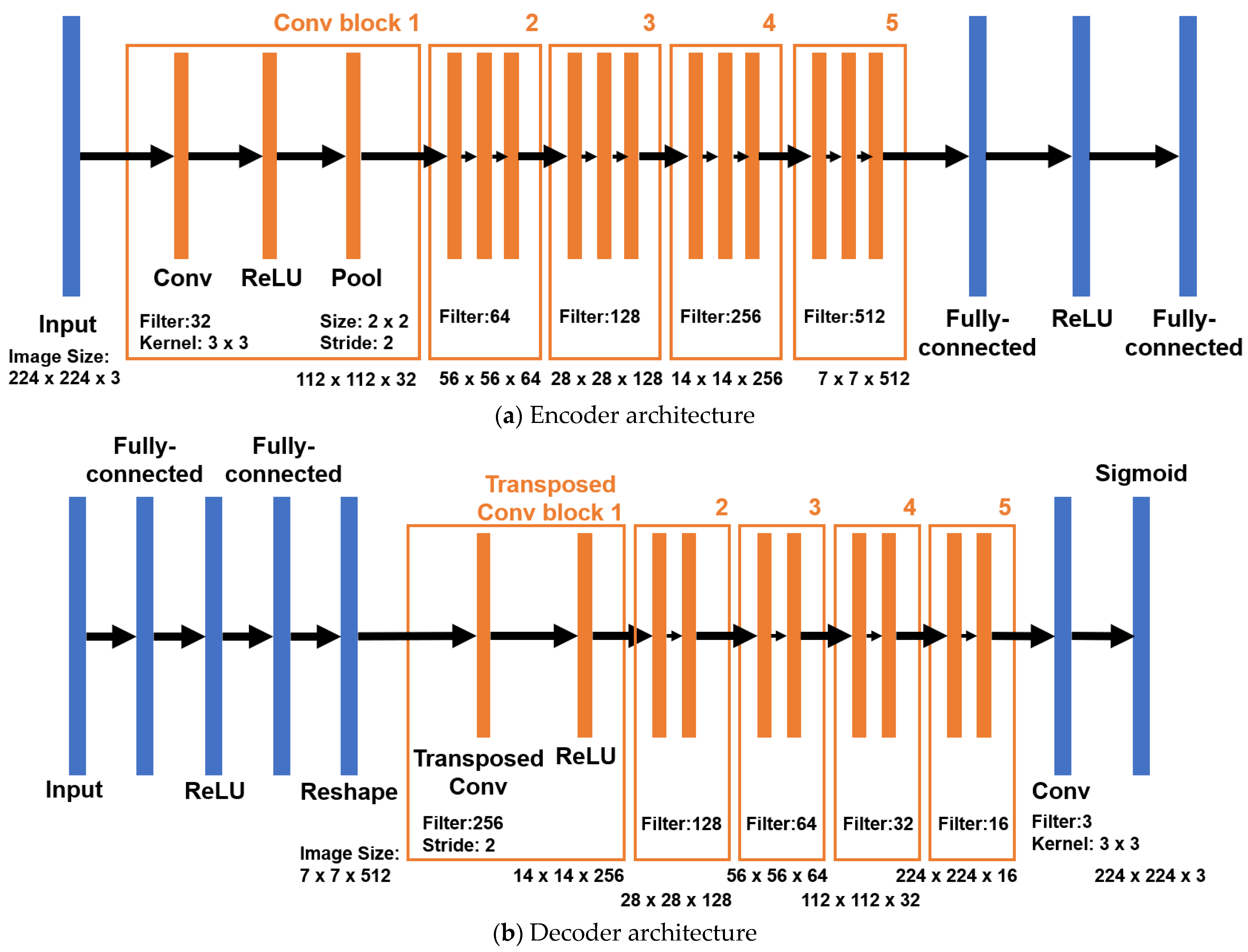
Figure 3 shows the architecture of the autoencoder used in this study. The number of convolutional blocks is set to 5, resulting in a relatively shallow configuration. This design choice was made to encourage the model to capture global spatial features rather than extracting local features, as the characteristics of a normal pattern can vary due to factors such as internal convection conditions [34]. Moreover, prior studies have demonstrated that applying k-means clustering to the latent space generated by the encoder is an effective method for unsupervised classification [35,36]. Accordingly, this established methodology was adopted in this study. The objective function for the autoencoder is to minimize the Root-Mean-Square Error (RMSE) on the validation data. To achieve this objective, hyperparameter optimization was performed using 50 Bayesian optimization trials with the Adam optimizer. The optimization focused on key parameters known to influence performance significantly: the dimensionality of the latent space, the number of nodes in the FC layer following the convolutional blocks, the learning rate, the mini-batch size, and the number of epochs [31,37,38]. The threshold for anomaly detection was determined using the three-sigma method, which relies solely on the statistical properties of the normal data. This approach not only enhances generalization but also ensures reliability by theoretically constraining the false positive rate to approximately 0.3% or less. For the autoencoder, the total normal dataset (2800 images) was partitioned, utilizing 80% for training and 10% for validation. Its performance was subsequently evaluated on a test set comprising the remaining 10% of normal data (280 images) and the entire anomalous dataset (5600 images). In contrast, for K-Means classification, both the standard dataset (2800 images) and the anomalous datasets (200 images for each of the 28 patterns) were partitioned into training (80%), validation (10%), and testing (10%) sets, consistent with the data split used for the CNN.

3. Results and Discussion

3.1. Phased-Array Ultrasonic Testing Image Results

The dataset used in this study consisted of 2800 images representing normal patterns and 200 images for each of the 28 distinct anomalous patterns. Consequently, the total anomalous dataset comprises 5600 images. A representative example of an acquired phased array ultrasonic image is shown in Figure 4.
Under all tested conditions, some strong signals are observed near the first copper piping proximal to the probe. However, due to attenuation of the ultrasonic wave, this signal diminishes significantly in the subsequent copper piping, becoming almost indiscernible to human eyes near the seventh piping. In the “No Hole” case, faint signals are visible to the right of the center and in the left area of the image. These are hypothesized to be caused by side lobes. Side lobes are secondary radiation lobes that spread in lateral or oblique directions relative to the main beam. Several observations support this hypothesis. First, these signals are eliminated when a 100 mm wide stainless steel plate is placed between the copper piping. Given its width, this plate not only obstructs direct signal transmission between the piping but also attenuates ultrasonic waves propagating through the surrounding water. This suggests that the side lobe path is not a direct reflection between adjacent piping; instead, the ultrasonic waves appear to travel through the wider surrounding area, curve along the way, and then reflect off a piece of piping before returning to the probe. Second, the position of the signals does not change when the probe’s height is adjusted, making it unlikely that they are reflections from the bottom or wall surfaces. These findings collectively suggest that the observed faint signals are attributable to side lobes. In the “West” image, the bubble signal is readily identifiable in the lower left section. Similarly, in the “East” image, the bubble signal is clearly visible in the lower right. For the “North” condition, bubbles are emitted from the seventh copper piping and flow toward the top of the image. Although the emission point from the hole is not directly visible due to the attenuation of the ultrasonic wave, it is evident that the bubbles collide with the sixth copper piping and disperse across the upper region of the image. In the “South” case, a flow of bubbles is present toward the lower part of the image from the seventh copper piping. However, the ultrasonic wave is significantly attenuated, making direct signal identification difficult. Furthermore, for north or south emissions, visual identification of the source pipe is exceptionally difficult because the bubbles collide with adjacent pipes and disperse, resulting in only a marginal spatial shift. These results indicate that there are conditions in which it is difficult for human eyes to distinguish between normal and anomalous data. Therefore, it is necessary to apply ML for effective anomaly detection.

3.2. Bubble Detection Using a CNN with EfficientNet-b0

3.2.1. CNN Training Results

Based on Bayesian optimization, the model was trained with the following hyperparameters: a mini-batch size of 16, an epoch of 31, and a learning rate of 8.9 × 10⁻⁵. At the fourth iteration of Bayesian optimization, the classification error rate reached zero, confirming sufficient convergence. The learning curves in Figure 5 confirm that the CNN model was effectively trained. This is evidenced by the increase in accuracy and decrease in loss as the number of iterations increases. The model achieved a test accuracy of 100%, indicating a perfect classification with no errors. While identifying the specific type of anomaly can be difficult with ultrasonic testing alone, this CNN model enables precise characterization. It detects not only the presence or absence of bubbles but also identifies the specific copper piping from which they originated and the direction from which they are emitted. Such precise information would enable a more rapid and effective response to operational issues in an actual plant.

3.2.2. CNN Model Explainability

Significant progress has been made in detecting sodium-water reactions in fast reactor steam generators using ML. For instance, Mikami et al. demonstrated that deep learning can classify normal piping acoustics and bubble-jet noise under simulated anomalous conditions with an extremely high accuracy of 99.76% [1]. Furthermore, Marklund et al. applied Hidden Markov Models (HMMs) to demonstrate that leak signals can be detected even in low signal-to-noise ratio (SNR) environments using actual plant data [6]. The CNN developed in this study also demonstrated high detection performance, consistent with prior work. However, these high-performance models share a common challenge across the nuclear field, AI research, and other sectors. This challenge is the lack of explainability in their internal decision-making processes, which function as “black boxes” [39,40]. This lack of transparency in the prediction process is a significant barrier to operators’ trust in and use of AI outputs in practical operations, especially in the nuclear field, where safety is paramount. This lack of “Explainability” is recognized as a cross-disciplinary challenge in the application of ML to critical societal infrastructure. Therefore, this study aims not only to improve detection performance but also to fundamentally enhance system reliability. Specifically, to visualize the basis for the CNN’s judgments, the Gradient-weighted Class Activation Mapping (Grad-CAM) method is applied to the CNN model. Furthermore, using t-distributed Stochastic Neighbor Embedding (t-SNE), the model’s classification features were visualized. This visualization will verify whether the model successfully captures distinct acoustic features corresponding to each anomalous pattern [41,42]. In this study, the Grad-CAM method was applied to data for which the predicted label matched the actual label. As shown in the following equation, the importance weights for each feature map are calculated by first differentiating the raw output score for the target class y c (before the softmax function) with respect to the feature maps of the final convolutional layer A i j k , and applying global average pooling to these gradients [40].
α k c = 1 Z i j y c A i j k
A heatmap L G r a d C A M c is generated by computing a weighted linear combination with feature maps A k using these calculated weights α k c .
L G r a d C A M c = R e L U k α k c A k
This process is performed for each data point. To visualize the areas of importance for each class, the resulting heatmaps are averaged pixel-wise for each respective label.
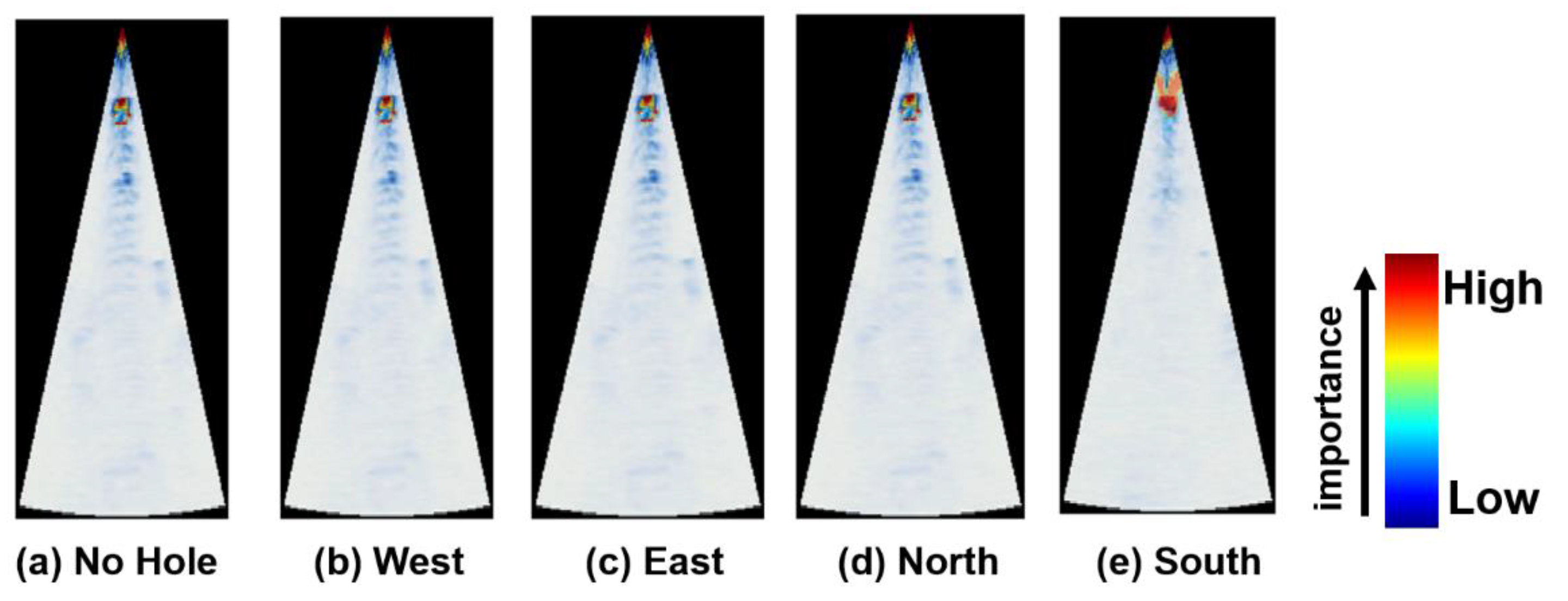
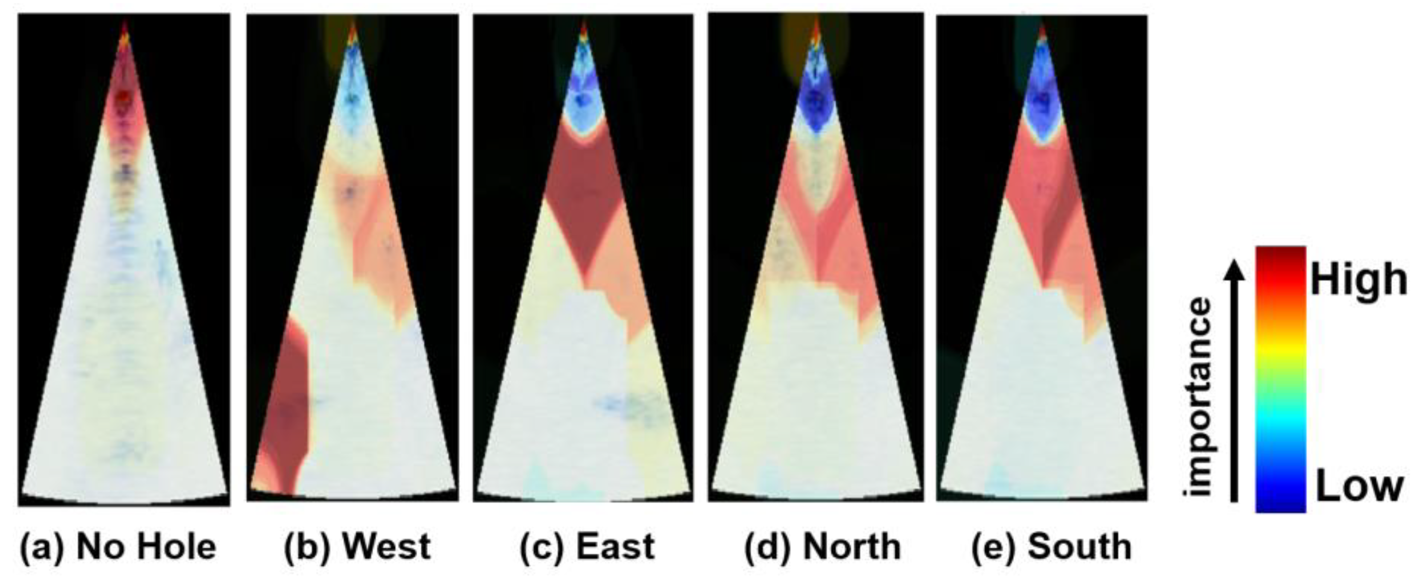
Figure 6 shows the average Grad-CAM results for the one normal pattern and four anomalous patterns in the seventh copper piping. In the “No Hole” condition, the central region of the sector-shaped ultrasonic image is identified as an important area. This observation suggests two hypotheses. The first is that the model is monitoring the region where bubbles would typically appear, thereby confirming their absence. The second hypothesis is that the model is tracking for the presence of a side lobe. If bubbles were to exist in an area superior to the side lobe’s propagation path, they would cause attenuation of the ultrasonic signal and eliminate the side lobe. Consequently, the model may be using the presence or attenuation of these side lobes as an indirect feature. The “West” condition accurately localizes the bubble region in the lower-left of the ultrasonic image, and the “East” condition correctly identifies the bubbles in the lower-right. In the “7-North” condition, excessive ultrasonic attenuation prevents direct observation of the bubble emission point; however, the model clearly captures the faint signals from bubbles that have collided with the sixth copper piping and dispersed into the upper region of the image. Similarly, for the “South” condition, the bubbles emitted from the seventh copper piping are not captured directly. Instead, it appears to identify the fluid flow toward the lower part of the image caused by the bubble emission, which explains the localization of the critical region in the upper area. These results demonstrate that the CNN model successfully determines the presence and location of bubble generation. It accomplishes this by using a diverse set of indicators, including direct bubble signals, signals from migrated bubbles, and even subtle signals associated with internal fluid flow.
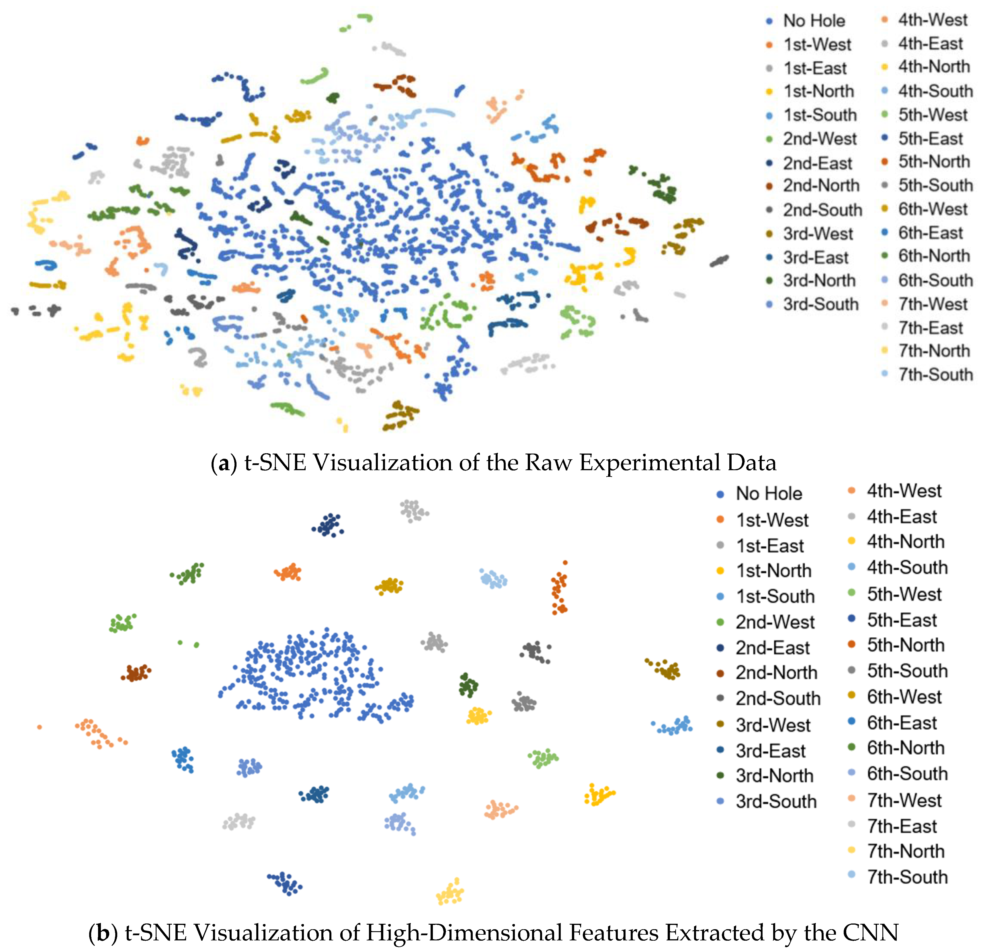
t-SNE is used to visualize whether the model successfully extracted distinct features for each class during training [41]. t-SNE method computes the similarity between images in a high-dimensional space and attempts to find a low-dimensional space embedding that preserves these similarities. Specifically, to evaluate similarities in the high-dimensional space, a degree of similarity is defined as follows [41].
p j | i = e x p x i x j 2 2 σ i 2 k i e x p x i x k 2 2 σ i 2 ,
where p j | i is the conditional probability of point j given point i in high-dimensional space, x is the data points in high-dimensional space, and σ i is the variance of the Gaussian kernel centered on point x . The bandwidth of the Gaussian kernel is determined by finding a value that makes the perplexity of the distribution equal to a user-specified value. This process creates a similarity matrix of high-dimensional space. Subsequently, to reproduce these similarities for visualization, the data features for each image are embedded at random positions in a low-dimensional space. The similarity between these points is then evaluated using a Student’s t-distribution, as shown in the equation below [41].
q i j = 1 + y i y j 2 1 k i 1 + y k y l 2 1 ,
where q i j is the joint probability between points i and j in low-dimensional space and y is the data points in low-dimensional space. The final t-SNE embedding is found by minimizing the Kullback–Leibler divergence between these two distributions using gradient descent. While this exact method is computationally intensive, the Barnes-Hut algorithm, which uses a tree-based structure to accelerate computation [42], is effective for larger datasets.
Perplexity was set to 15 consistently to ensure a uniform basis for comparing models. This value was selected because the influence on performance is negligible across the typical operating range of 5 to 50 [41]. A comparison of the visualizations in Figure 7 reveals a stark contrast. In the raw experimental data, the feature-space distinctions are ambiguous, with the normal and anomalous patterns, as well as the differences among the various anomalous classes, essentially indistinguishable. Conversely, it is evident that during feature extraction, the CNN successfully isolates and extracts salient class-specific features. This results in distinct, well-separated clusters in the t-SNE plot. This result confirms not only that the model’s classification basis is effective but also that it can identify and extract distinct, meaningful features for each class.

3.3. Bubble Detection Using Autoencoder

3.3.1. Detection of Unseen Anomalies

While the CNN, as mentioned above, can classify not only the presence of bubbles but also their specific emission locations and directions, it would struggle to identify anomalous conditions that were not simulated in this experiment. Therefore, to develop a system that can adapt to unknown anomalous patterns, an autoencoder is employed. This model is trained exclusively on normal data, aiming to classify any deviation from this learned normality as an anomaly.
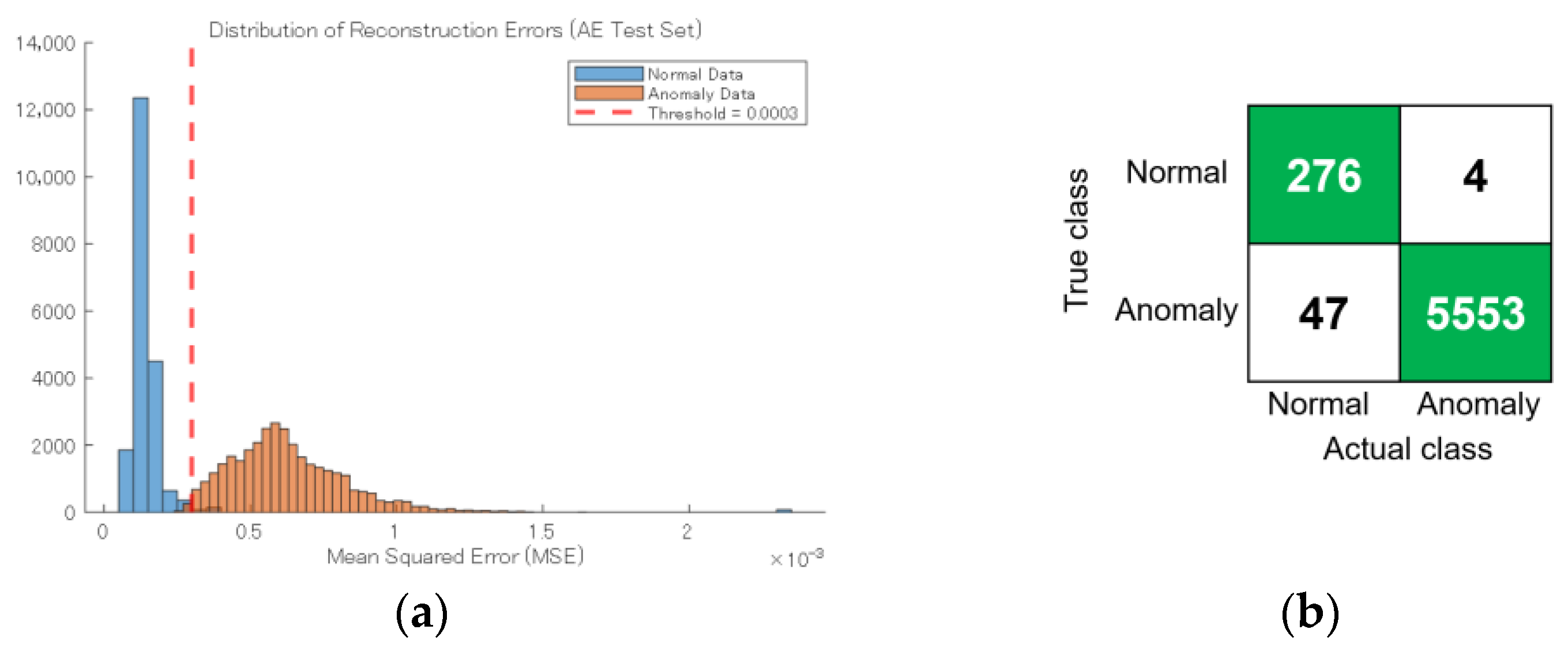
After 50 Bayesian optimization trials, with the objective function set to minimize reconstruction error, the optimal hyperparameters were determined: a Latent dimension of 15, 59 epochs, a batch size of 8, a learning rate of 8.8 × 10⁻⁴, and 131 units in the FC. At the 39th iteration of Bayesian optimization, the validation RMSE reached a minimum of 4.57, confirming sufficient convergence. The reconstruction error threshold for distinguishing between normal and anomalous data was calculated to be 3.0 × 10⁻⁴, using the three-sigma method on the normal validation set, as shown in Figure 8. A sensitivity analysis (σ = 0 and 10) demonstrated the setting’s validity, as recall and anomaly counts remained stable between σ = 0 and 3. The final anomaly detection accuracy was 99.1%. The model’s successful detection of 28 unseen anomalous patterns suggests its capacity for generalization to anomalous conditions not reproduced in the experiment. Furthermore, since the image pixel values were normalized to the [0, 1] range, the validation RMSE of 0.01191 indicates that the model reconstructed the normal validation data with an error of approximately 1.2%. The overall test RMSE, which included both normal and anomalous data, was 0.02454. This higher value is attributable to significantly larger reconstruction errors for the anomalous data, thereby validating the model’s ability to differentiate between the two classes effectively.

3.3.2. Autoencoder Explainability and Feature Extraction

The Grad-CAM method can be applied by calculating gradients with respect to a specific class score [40]. An autoencoder, however, does not output class-specific scores; instead, it outputs the reconstruction error, a global metric rather than a class-specific one. Therefore, to visualize the model’s decision-making basis, the Local Interpretable Model-agnostic Explanations (LIME) method is employed in this study. LIME is a model-agnostic technique that can be applied regardless of the model’s internal architecture, as it approximates the model’s predictions with a linear function [39]. When determining the linear approximation, fidelity loss is calculated as shown in the equation below. This metric quantifies the extent to which the simple linear model fails to replicate the original, complex autoencoder.
L f ,   g ,   π x = z Z π x z f z g ( z ) 2 ,
where L ( f ,   g ,   π x ) is the fidelity loss, π x z is the proximity measures relative to instance x , f z is the prediction of the original model for instance z and g z is the Prediction of the simple model for instance z .
The LIME method is sensitive to several hyperparameters, necessitating careful selection [43]. In this study, the optimal values were determined for the kernel width (0.25, 0.50, or 0.75), segmentation method, and its associated parameters. When using Simple Linear Iterative Clustering (SLIC), the number of superpixels was tested at 25, 50, and 100. When using the Watershed Algorithm, the gradient minima suppression level was attempted at 0.1, 0.08, and 0.05. The number of perturbation samples generated was held at 1000. To determine the optimal parameters, an exhaustive search was performed over the defined hyperparameter range. This process was applied to correctly classified images for five labels to ultimately output an averaged LIME importance map. The evaluation flow proceeded in three stages. First, a stability check was used as a cut-off. LIME was executed seven times on the same image, and the average standard deviation of the superpixel importance was calculated [43,44]. If this average exceeded 0.05, the set was discarded. Second, the remaining sets were ranked by fidelity, which was evaluated by calculating the infidelity (the discrepancy between the original model’s predictions and the surrogate model’s predictions by LIME on the perturbation samples) [43,44]. Finally, the top-ranked, high-fidelity combinations were qualitatively reviewed by a human eye to select the set that provided the most plausible and interpretable explanations. Following this evaluation, the optimal hyperparameter was determined to be SLIC as the segmentation method, a kernel width of 0.75, and a superpixel count of 50.
Figure 9 reveals that the region identified as necessary for anomaly detection is consistently a narrow area at the top of the image across all classes, including the normal pattern and the anomalous ones. Furthermore, when employing the SLIC segmentation method, the decision basis exhibited no significant sensitivity to variations in the kernel width or the number of superpixels. This is a critical finding, as each label corresponds to a unique experimental condition with a different anomaly location and direction. Consequently, the crucial regions were expected to differ across classes, but they did not. This discrepancy suggests that the autoencoder may be capturing a subtle fluid flow near the probe rather than identifying the bubbles.

3.3.3. Identifying Anomaly Location and Direction Using an Autoencoder and K-Means

While an autoencoder is effective for anomaly detection, it struggles with multi-class classification. However, by applying k-means to the latent space generated by the encoder, which captures the most salient features of the data, accurate classification can be achieved [35,45]. The k-means assigns data to clusters and aims to minimize the sum of squared distances between each data point and its assigned cluster centroid, as defined by the objective function below:
I = l = 1 K h C l h   μ l 2 ,
where K is the total number of clusters, l is the cluster index, h is a data point, μ l is the centroid of cluster l and C l is the set of all data points in cluster l . In this study, both the standard and anomalous datasets were partitioned into training (80%), validation (10%), and testing (10%) subsets. To mitigate the risk of falling into local minima and minimize the risk of initialization dependency, the best result was selected from 5 k-means++ trials.
Table 2 shows the performance of k-means applied to the features extracted from the encoder. The overall test accuracy was 46.3%, and the macro F1-score was 0.164, indicating that this model struggled with multi-class classification. In contrast, the normal (“No Hole”) class achieved high precision and recall, resulting in a high F1-score. However, for specific anomalous patterns, such as “1-East,” zero correct predictions were made. These results suggest that while the model can effectively detect the presence or absence of bubbles, it struggles to identify the specific mechanism of bubble generation.

3.4. Anomaly Detection and Multi-Class Classification by Autoencoder-Based Feature Extraction

3.4.1. Autoencoder Limitations in Rationale and Classification and Proposed Method

Figure 10 shows examples of input images to the autoencoder and their corresponding reconstructed output images. Because the model was trained to reconstruct normal data, the reconstructed normal images are visually identical to the experimental ones. However, focusing on the anomalous data reveals that the signals corresponding to bubbles have been removed or suppressed during reconstruction. This implies that the latent features—the encoder’s output—also lack the critical features associated with bubble signals. This would explain the previously observed issues: the poor performance of k-means and the inappropriate decision rationale identified by LIME. This failure is likely because the autoencoder, which optimizes for whole reconstruction error, failed to adequately learn these small anomalous features, as the bubble region is extremely small relative to the entire image. Prior research indicates that clustering using latent features extracted by an autoencoder can yield superior performance compared to methods that rely solely on reconstruction error [46,47,48,49,50,51].
Therefore, the objective of this study is to enhance the classification accuracy of anomaly location and direction, while simultaneously ensuring that anomaly detection is grounded in a sound, interpretable decision-making basis [50]. To achieve our objective, an autoencoder was leveraged as a feature extractor, and its encoder latent features will be used for both anomaly detection (One Class Support Vector Machine (SVM)) and classification of anomaly types (k-means). Furthermore, in this approach, both normal and anomalous data are intentionally input into the autoencoder without labels. The goal is to leverage the learning process by allowing the model to extract common, underlying features from both data types. The point of this proposed method lies in its simultaneous integration of three specific components. First, this architecture employs Bayesian optimization to tune the autoencoder’s hyperparameters by maximizing the validation Area Under the Curve (AUC) of a subsequent One-Class SVM trained on the autoencoder’s latent features. Second, the latent features extracted from this encoder are subsequently input into k-means to classify the specific types of anomalies. Third, both normal and anomalous data are intentionally fed into the autoencoder without labels, allowing the model to learn the underlying standard features. The autoencoder architecture itself remains the same as previously described. For the feature extraction phase, 80% of the normal data (2240 images) and 80% of the anomalous data (40 images per pattern) were used. For the anomaly detection phase, 80% of the normal data (2240 images) was employed. Finally, validation and testing were evaluated using 10% of the normal data (280 images) and 10% of the anomalous data (560 images), respectively.
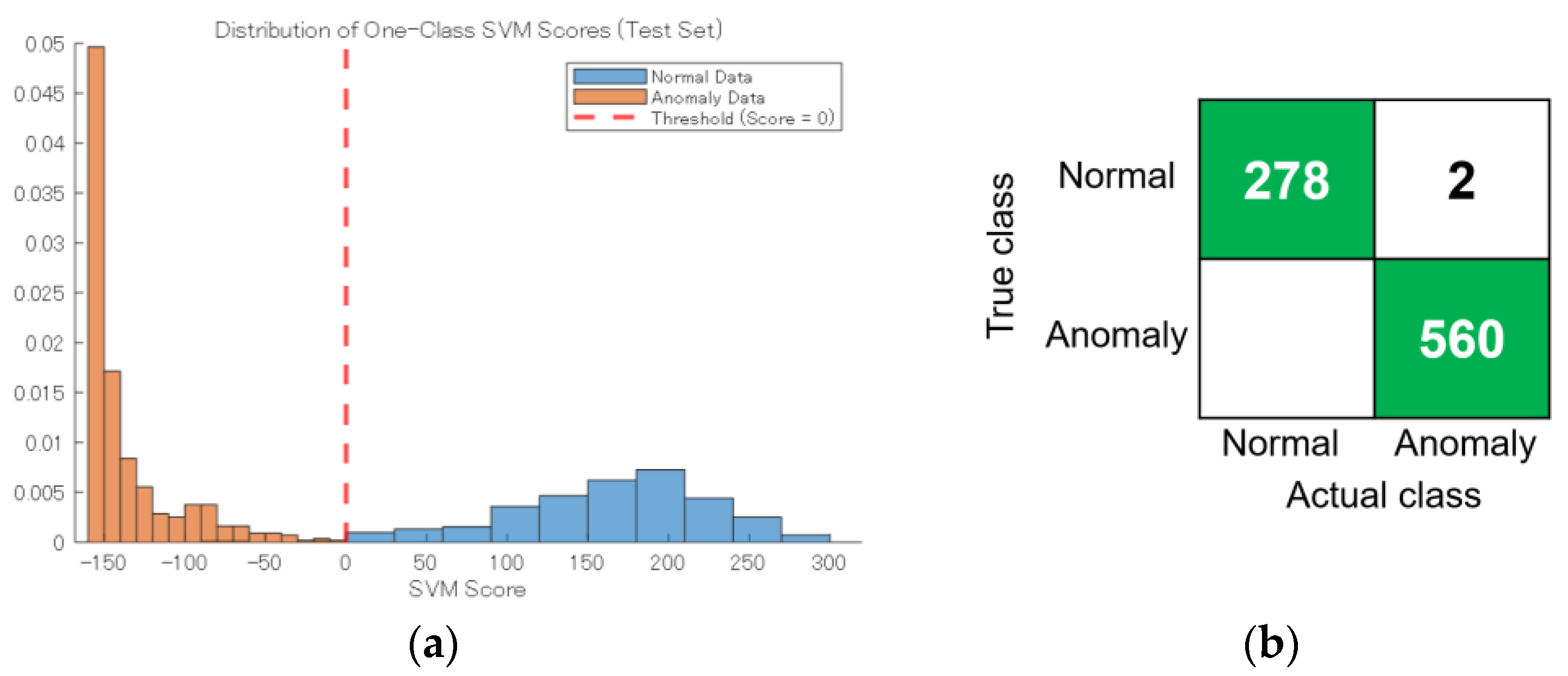
Figure 11 shows the anomaly score distribution for the test data and the resulting confusion matrix for the One Class SVM anomaly detection. To establish non-linear boundaries by mapping data into a high-dimensional space, a Gaussian kernel was utilized to define the decision boundary for the normal data [52]. The Outlier Fraction was set to 0.01, and the Kernel Scale was determined automatically using the ‘auto’ setting in MATLAB (versions R2025b) [52,53]. A grid-based approach was employed to conduct a sensitivity analysis and evaluate the impact of these hyperparameters. A total of 54 combinations were tested, varying the Outlier Fraction from 0.001 to 0.1 and the Kernel Scale from 0.25 to 4. The resulting standard deviation of the AUC was 2.18 × 10⁻⁴, indicating that hyperparameter sensitivity was negligible. This model’s hyperparameters were determined via 50 Bayesian optimization trials, with the validation set AUC maximized as the objective function. At the 20th iteration, the validation AUC reached 0.999, confirming sufficient convergence. The optimal values were found to be a latent dimension of 5 (from a range of 4 to 128), 222 units in the FC (from 128 to 384), a learn rate of 5.29 × 10⁻⁴ (from 1.0 × 10⁻⁵ to 1.0 × 10⁻²), a batch size of 8 (4, 8, 16, 32, 64), 40 epochs (from 5 to 60). The score distribution clearly illustrates that nearly all data points are correctly classified using a threshold of 0 as the decision boundary. The model achieved a test accuracy of 99.8%, representing a significant improvement over the previous autoencoder-only method.

3.4.2. Identifying Anomaly Location and Direction by Autoencoder and One Class SVM

To visualize the decision-making basis, the LIME method was employed. The hyperparameters for LIME were selected using the same methodology as for the autoencoder, with identical hyperparameter types, search ranges, and selection criteria based on stability and fidelity. In this trial, the LIME objective function was set to the One Class SVM score. This optimization process resulted in the following optimal parameters: SLIC as the segmentation method, a kernel width of 0.75, and a superpixel count of 50.
Figure 12 illustrates the criteria for the anomaly detection performed by the One-Class SVM, which used features extracted from the autoencoder. The visualization shows the average classification accuracy for correctly classified data (i.e., when the prediction matched the true label) for each class. In the normal (“No Hole”) condition, the critical regions are localized around the probe and the periphery of the copper piping array, suggesting the model is actively monitoring these areas to confirm the absence of bubbles. For the West pattern, a high degree of importance is correctly placed on the bubble signal. Similarly, East also shows the bubble location as the critical region. In the North condition, the model identifies the upper area of the image where bubbles have dispersed after colliding with the sixth pipe. For South, consistent with the previous CNN results (Figure 6), the model appears to capture the fluid flow associated with bubble emission rather than the bubbles themselves. Considering these results comprehensively, while some challenges with the decision criteria persist, this represents an improvement compared to the decision criteria of the autoencoder-only method shown in Figure 9. Furthermore, when employing the SLIC segmentation method, the decision basis exhibited no significant sensitivity to variations in the kernel width or the number of superpixels.

3.4.3. K-Means Multi-Class Classification by Autoencoder-Based Feature Extraction

Table 3 shows the results of the K-means classification applied to the latent features extracted by the autoencoder to classify bubble generation location and direction. The analysis conditions were consistent with the previous autoencoder, specifying 29 classes for K-means. In this study, both the normal (2800 images) and anomalous datasets (200 images for each of the 28 patterns) were partitioned into training (80%), validation (10%), and testing (10%) subsets, consistent with the data split used for the CNN. The overall test accuracy was 74.5%, and the macro F1-score improved dramatically from 0.164 to 0.559. Furthermore, recall was generally higher than precision. This is a favorable outcome for adaptation to an actual plant, as it indicates a lower probability of false negatives. Additionally, classes that previously had an F1-score of 0.00, such as “1-East,” “3-East,” and “6-West,” showed significant improvement, with their scores increasing to 0.884, 1.00, and 1.00, respectively. Nevertheless, challenges persist, as the F1-scores for “3-West” and “4-East” remained at 0.00.

3.4.4. Comparison with the Autoencoder Using Per-Class Feature Visualization

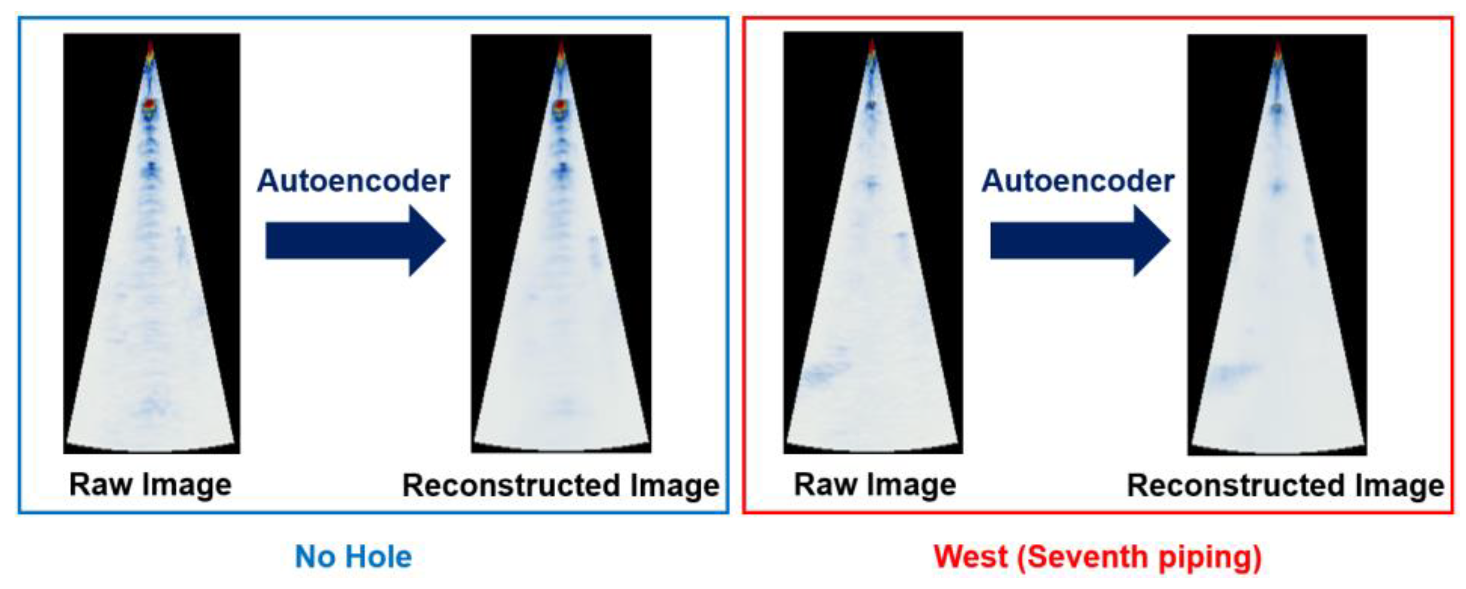
Figure 13 shows an example comparison between the input experimental images and the corresponding reconstructed images from this model’s autoencoder decoder. In sharp contrast to the previous autoencoder trained only on normal data (Figure 10), it is evident that the signals corresponding to the bubbles are not removed; instead, they are adequately reconstructed. This indicates that the crucial features of the bubbles are preserved within the latent features at the encoder’s output. This preservation of features enables subsequent One Class SVM and k-means models to effectively leverage this information for classification, resulting in a dramatic increase in accuracy.
Figure 14 contrasts the feature separation capabilities of two different models. (a) and (c) show the results for anomaly detection and anomaly type identification, using the autoencoder-only method. In contrast, (b) and (d) show the results for the proposed method, which utilizes the autoencoder as a feature extractor. The t-SNE results were computed using the encoder’s latent features as input. A comparison of (a) and (b) reveals that while the autoencoder-only method shows significant overlap between normal and anomalous data, the proposed method reduces this overlap. This indicates that, by intentionally feeding both normal and anomalous data to the encoder without labels, the model learns common, essential features that must be preserved. The latter approach is more effective at extracting features unique to each class. A similar comparison between (c) and (d) confirms that the proposed method is also superior at extracting specific features for each distinct anomaly type. These results validate the proposed methodology, which combines input from both normal and anomalous data using a hybrid objective function (minimizing reconstruction error while maximizing the One Class SVM’s AUC). Furthermore, this approach demonstrates strong generalization, comparable to or exceeding that of the CNN. This is because the feature extraction during autoencoder training is trained on unlabeled data. Moreover, the One Class SVM anomaly detector is trained only on the latent features of normal data. Consequently, the proposed method achieves both high test accuracy and strong generalization. This demonstrates that the model not only enables the identification of anomaly types—which is difficult with conventional ultrasonic methods—but also possesses a higher generalization capability than the CNN.

4. Conclusions

In this study, we successfully confirmed the presence of bubbles. We accurately identified their generation location and direction using a CNN, with the bubbles themselves as the basis for decision-making. Furthermore, we demonstrated successful anomaly detection for previously unseen anomalies by training an autoencoder solely on normal data. However, this autoencoder method revealed issues with a flawed decision basis and the use of inappropriate features. To address this, we proposed a technique in which the autoencoder was leveraged as a feature extractor, trained on both normal and anomalous data to learn their common underlying features. By combining this with a One-Class SVM and k-means clustering, we identified the location and direction of bubble generation without requiring labeled anomaly data. This methodology shows significant potential for application in the anomaly-detection systems of fast-reactor steam generators, PWR cores, and LNG regasification units. To further assess its viability for practical implementation in an actual plant, future work must validate the model’s performance across various noise environments, turbulence conditions, and different types of fluids.

Author Contributions

Conceptualization, Y.O., S.N., Y.K. and M.F.; methodology, Y.O.; formal analysis, Y.O.; investigation, Y.O.; visualization, Y.O.; writing—original draft preparation, Y.O.; writing—review and editing, S.N. and M.F. All authors have read and agreed to the published version of the manuscript.

Funding

This research received no external funding.

Institutional Review Board Statement

Not applicable.

Informed Consent Statement

Not applicable.

Data Availability Statement

The original data presented in this study are contained in this manuscript. Further inquiries may be directed to the corresponding author.

Acknowledgments

We are grateful to Kunihiko Nabeshima and Hiroki Yada of Japan Atomic Energy Agency (JAEA) and Keisuke Uchida of Tohkou Machine Industry Co., Ltd. for their advice. Generative AI (Gemini 2.5 Pro and Gemini 3 Pro, Google LLC) was used to aid in the translation and refinement of the manuscript’s language.

Conflicts of Interest

The authors declare no conflicts of interest.

Nomenclatures

AUCArea Under the Curve
CHFCritical Heat Flux
CNNConvolutional Neural Network
FCFully Connected (layer)
Grad-CAMGradient-weighted Class Activation Mapping
HMMHidden Markov Model
LIMELocal Interpretable Model-agnostic Explanations
LNGLiquefied Natural Gas
MLMachine Learning
ORVOverpressure Relief Valve
PWRPressurized Water Reactor
RMSERoot Mean Square Error
RPTReactor Pressure Test
SLICSimple Linear Iterative Clustering
SNRSignal-to-Noise Ratio
SVMSupport Vector Machine
t-SNEt-distributed Stochastic Neighbor Embedding
UTUltrasonic Testing
Roman symbols
A i j k Value at position of the k-th feature map
C l Set of all data points in cluster l
f z Prediction of the original model for instance z
g z Prediction of the simple model for instance z
hA data point
KTotal number of clusters
L ( f ,   g ,   π x ) Fidelity loss
L G r a d C A M c Grad-CAM heatmap for class c
l Cluster index
p j | i Conditional probability of point j given point i in high-dimensional space
q i j Joint probability between points i and j in low-dimensional space
tTemperature
xData points in high-dimensional space
yData points in low-dimensional space
y c Score for class c
ZAcoustic impedance
Greek symbols
α k c Weight of the k-th feature map for class c
μ l Centroid of cluster l
π x ( z ) Proximity measures relative to instance x
ρDensity
σ i Variance of the Gaussian kernel centered on point i
υSound velocity

References

  1. Mikami, N.; Ueki, Y.; Shibahara, M.; Aizawa, K.; Ara, K. State Sensing of Bubble Jet Flow Based on Acoustic Recognition and Deep Learning. Int. J. Multiph. Flow 2023, 159, 104340. [Google Scholar] [CrossRef]
  2. Korolev, I.; Aliev, T.; Orlova, T.; Ulasevich, S.A.; Nosonovsky, M.; Skorb, E.V. When Bubbles Are Not Spherical: Artificial Intelligence Analysis of Ultrasonic Cavitation Bubbles in Solutions of Varying Concentrations. J. Phys. Chem. B 2022, 126, 3161–3169. [Google Scholar] [CrossRef]
  3. Sun, S.; Xu, F.; Cai, L.; Salvato, D.; Dilemma, F.; Capriotti, L.; Xian, M.; Yao, T. An Efficient Instance Segmentation Approach for Studying Fission Gas Bubbles in Irradiated Metallic Nuclear Fuel. Sci. Rep. 2023, 13, 22275. [Google Scholar] [CrossRef] [PubMed]
  4. Liu, Z.; Niu, X.; Guo, X.; Mu, G.; Pang, Y. Method for Acoustic Leak Detection of Fast Reactor Steam Generator Based on Wavelet Noise Elimination. In Proceedings of the 2006 International Conference on Machine Learning and Cybernetics, Dalian, China, 13–16 August 2006; pp. 957–961. [Google Scholar]
  5. Brunet, M.; Garnaud, P.; Ghaleb, D.; Kong, N. Water Leak Detection in Steam Generator of Super Phenix. Prog. Nucl. Energy 1988, 21, 537–544. [Google Scholar] [CrossRef]
  6. Riber Marklund, A.; Michel, F.; Anglart, H. Demonstration of an Improved Passive Acoustic Fault Detection Method on Recordings from the Phénix Steam Generator Operating at Full Power. Ann. Nucl. Energy 2017, 101, 1–14. [Google Scholar] [CrossRef]
  7. Yoshitaka, C. Acoustic Leak Detection System for Sodium-Cooled Reactor Steam Generators Using Delay-and-Sum Beamformer. J. Nucl. Sci. Technol. 2010, 47, 103–110. [Google Scholar] [CrossRef]
  8. Yamamoto, T.; Kato, A.; Hayakawa, M.; Shimoyama, K.; Ara, K.; Hatakeyama, N.; Yamauchi, K.; Eda, Y.; Yui, M. Fundamental Evaluation of Hydrogen Behavior in Sodium for Sodium-Water Reaction Detection of Sodium-Cooled Fast Reactor. Nucl. Eng. Technol. 2024, 56, 893–899. [Google Scholar] [CrossRef]
  9. Mathews, C.K. Liquid Sodium—The Heat Transport Medium in Fast Breeder Reactors. Bull. Mater. Sci. 1993, 16, 477–489. [Google Scholar] [CrossRef]
  10. Mingyu, H.; Tao, W.; Jinbing, C.; Xiaoran, W. Study on Ultrasonic Location Based on Sound Pressure and TDOA Switching. In Proceedings of the 2020 Chinese Control and Decision Conference (CCDC), Hefei, China, 22–24 August 2020; IEEE: New York, NY, USA, 2020; pp. 3153–3158. [Google Scholar]
  11. Griffin, J.W.; Peters, T.J.; Posakony, G.J.; Chien, H.-T.; Bond, L.J.; Denslow, K.M.; Sheen, S.-H.; Raptis, P. Under-Sodium Viewing: A Review of Ultrasonic Imaging Technology for Liquid Metal Fast Reactors; Pacific Northwest National Laboratory (PNNL): Richland, WA, USA, 2009.
  12. Massacret, N.; Ploix, M.A.; Corneloup, G.; Jeannot, J.P. Modelling of Ultrasonic Propagation in Turbulent Liquid Sodium with Temperature Gradient. J. Appl. Phys. 2014, 115, 204905. [Google Scholar] [CrossRef]
  13. Barathula, S.; Srinivasan, K. Review on Research Progress in Boiling Acoustics. Int. Commun. Heat Mass Transf. 2022, 139, 106465. [Google Scholar] [CrossRef]
  14. Shumskii, B.E.; Vorob’eva, D.V.; Mil’to, V.A.; Semchenkov, Y.M. Investigation of Spatial Effects Accompanying Local Boiling of Coolant in VVER Core on the Basis of Neutron Flux Noise Analysis. Energy 2019, 126, 345–350. [Google Scholar] [CrossRef]
  15. Shu, L.; Zhu, X.; Huang, X.; Zhou, Z.; Zhang, Y.; Wang, X. A Review of Research on Acoustic Detection of Heat Exchanger Tube. EAI Endorsed Trans. Ind. Netw. Intell. Syst. 2015, 2, e5. [Google Scholar] [CrossRef]
  16. Hu, Z.; Xu, L.; Chien, C.-Y.; Yang, Y.; Gong, Y.; Ye, D.; Pacia, C.P.; Chen, H. Three-Dimensional Transcranial Microbubble Cavitation Localization by Four Sensors. IEEE Trans. Ultrason. Ferroelectr. Freq. Control 2021, 68, 3336–3346. [Google Scholar] [CrossRef] [PubMed]
  17. Hans, R.; Dumm, K. Leak Detection of Steam or Water into Sodium in Steam Generators of Liquid-Metal Fast Breeder Reactors. At. Energy Rev. 1977, 15, 611–699. [Google Scholar]
  18. Desai, P.D.; Ng, W.C.; Hines, M.J.; Riaz, Y.; Tesar, V.; Zimmerman, W.B. Comparison of Bubble Size Distributions Inferred from Acoustic, Optical Visualisation, and Laser Diffraction. Colloids Interfaces 2019, 3, 65. [Google Scholar] [CrossRef]
  19. Shung, K.K. High Frequency Ultrasonic Imaging. J. Med. Ultrasound 2009, 17, 25–30. [Google Scholar] [CrossRef] [PubMed]
  20. Wajman, R. Computer Methods for Non-Invasive Measurement and Control of Two-Phase Flows: A Review Study. Inf. Technol. Control 2019, 48, 464–486. [Google Scholar] [CrossRef]
  21. Boháčik, M.; Mičian, M.; Sládek, A. Evaluating the Attenuation in Ultrasonic Testing of Castings. Arch. Foundry Eng. 2018, 18, 151–156. [Google Scholar] [CrossRef]
  22. Matz, V.; Kreidl, M.; Smid, R. Classification of Ultrasonic Signals. Int. J. Mater. Prod. Technol. 2006, 27, 145–155. [Google Scholar] [CrossRef]
  23. Guichou, R.; Tordjeman, P.; Bergez, W.; Zamansky, R. Experimental Study of Bubble Detection in Liquid Metal. In Proceedings of the VIII International Scientific Colloquium “Modelling for Materials Processing”, Riga, Latvia, 21–22 September 2017; Volume 53, p. 667. [Google Scholar]
  24. Sun, H.; Ramuhalli, P.; Meyer, R. An Assessment of Machine Learning Applied to Ultrasonic Nondestructive Evaluation; Oak Ridge National Laboratory (ORNL): Oak Ridge, TN, USA, 2023.
  25. Zhang, X.; Yu, Y.; Yu, Z.; Qiao, F.; Du, J.; Yao, H. A Scoping Review: Applications of Deep Learning in Non-Destructive Building Tests. Electronics 2025, 14, 1124. [Google Scholar] [CrossRef]
  26. Matsuura, M.; Ikeda, M. Modification of Steam Generator System to Prevent Overheating Tube Rapture Accidents at MONJU. In Proceedings of the 18th International Conference on Structural Mechanics in Reactor Technology, Beijing, China, 7–12 August 2005. [Google Scholar]
  27. Chetal, S.C. Evolution of Design of Steam Generator for Sodium Cooled Reactors; International Atomic Energy Agency: Vienna, Austria, 1997. [Google Scholar]
  28. Haynes, W.M. (Ed.) CRC Handbook of Chemistry and Physics; CRC Press: Boca Raton, FL, USA, 2016. [Google Scholar]
  29. Rusman, J. Klasifikasi Cacat Biji Kopi Menggunakan Metode Transfer Learning dengan Hyperparameter Tuning Gridsearch. J. Teknol. Dan Manaj. Inform. 2023, 9, 37–45. [Google Scholar] [CrossRef]
  30. Tan, M.; Le, Q. EfficientNetV2: Smaller Models and Faster Training. In Proceedings of the 38th International Conference on Machine Learning Research, Online, 18–24 July 2021; pp. 10096–10106. [Google Scholar]
  31. Chang, D.T. Bayesian Hyperparameter Optimization with BoTorch, GPyTorch, and Ax. arXiv 2019, arXiv:1912.05686. [Google Scholar]
  32. Ando, K.; Onishi, K.; Bale, R.; Tsubokura, M.; Kuroda, A.; Minami, K. Nonlinear Mode Decomposition and Reduced-Order Modeling for Three-Dimensional Cylinder Flow by Distributed Learning on Fugaku. In High Performance Computing, Proceedings of the ISC High Performance Digital 2021 International Workshops; Jagode, H., Anzt, H., Ltaief, H., Luszczek, P., Eds.; Springer International Publishing: Cham, Switzerland, 2021; Volume 12761, pp. 122–137. [Google Scholar]
  33. Ma, H.; Zhang, Y.; Haidn, O.J.; Thuerey, N.; Hu, X. Supervised Learning Mixing Characteristics of Film Cooling in a Rocket Combustor Using Convolutional Neural Networks. Acta Astronaut. 2020, 175, 11–18. [Google Scholar] [CrossRef]
  34. Serafim Rodrigues, T.; Rogério Pinheiro, P. Hyperparameter Optimization in Generative Adversarial Networks (GANs) Using Gaussian AHP. IEEE Access 2024, 13, 770–788. [Google Scholar] [CrossRef]
  35. Huang, P.; Yan, H.; Song, Z.; Xu, Y.; Hu, Z.; Dai, J. Combining Autoencoder with Clustering Analysis for Anomaly Detection in Radiotherapy Plans. Quant. Imaging Med. Surg. 2023, 13, 2328–2338. [Google Scholar] [CrossRef]
  36. Aktar, S.; Nur, A.Y. Advancing Network Anomaly Detection: An Ensemble Approach Combining Optimized Contractive Autoencoders and k-Means Clustering. In Proceedings of the 2024 IEEE 3rd International Conference on Computing and Machine Intelligence (ICMI), Mt Pleasant, MI, USA, 11 July 2024; IEEE: New York, NY, USA, 2024; pp. 1–5. [Google Scholar]
  37. Dumont, V.; Ju, X.; Mueller, J. Hyperparameter Optimization of Generative Adversarial Network Models for High-Energy Physics Simulations. arXiv 2022, arXiv:2208.07715. [Google Scholar] [CrossRef]
  38. Alarsan, F.I.; Younes, M. Best Selection of Generative Adversarial Networks Hyper-Parameters Using Genetic Algorithm. SN Comput. Sci. 2021, 2, 283. [Google Scholar] [CrossRef]
  39. Ribeiro, M.T.; Singh, S.; Guestrin, C. “Why Should I Trust You?”: Explaining the Predictions of Any Classifier. In Proceedings of the 22nd ACM SIGKDD International Conference on Knowledge Discovery and Data Mining, San Francisco, CA, USA, 13–17 August 2016; Association for Computing Machinery: New York, NY, USA, 2016; pp. 1135–1144. [Google Scholar]
  40. Selvaraju, R.R.; Cogswell, M.; Das, A.; Vedantam, R.; Parikh, D.; Batra, D. Grad-CAM: Visual Explanations from Deep Networks via Gradient-Based Localization. In Proceedings of the IEEE International Conference on Computer Vision, Venice, Italy, 22–29 October 2017; pp. 618–626. [Google Scholar]
  41. van der Maaten, L.; Hinton, G. Visualizing Data Using T-SNE. J. Mach. Learn. Res. 2008, 9, 2579–2605. [Google Scholar]
  42. Maaten, L. van der Accelerating T-SNE Using Tree-Based Algorithms. J. Mach. Learn. Res. 2014, 15, 3221–3245. [Google Scholar]
  43. Laguna, S.; Heidenreich, J.N.; Sun, J.; Cetin, N.; Al-Hazwani, I.; Schlegel, U.; Cheng, F.; El-Assady, M. ExpLIMEable: A Visual Analytics Approach for Exploring LIME. In Proceedings of the 2023 Workshop on Visual Analytics in Healthcare (VAHC), Melbourne, Australia, 22 October 2023; pp. 27–33. [Google Scholar] [CrossRef]
  44. Anwar, S.; Griffiths, N.; Bhalerao, A.; Popham, T.J. MASALA: Model-Agnostic Surrogate Explanations by Locality Adaptation. In Proceedings of the 1st KDD Workshop on Human-Interpretable AI, Barcelona, Spain, 26 August 2024. [Google Scholar]
  45. Marquina-Araujo, J.J.; Cotrina-Teatino, M.A.; Cruz-Galvez, J.A.; Noriega-Vidal, E.M.; Vega-Gonzalez, J.A. Application of Autoencoders Neural Network and K-Means Clustering for the Definition of Geostatistical Estimation Domains|IIETA. Math. Model. Eng. Probl. 2024, 11, 1207. [Google Scholar] [CrossRef]
  46. Nguyen, V.; Viet Hung, N.; Le-Khac, N.-A.; Cao, V.L. Clustering-Based Deep Autoencoders for Network Anomaly Detection; Springer International Publishing: Berlin/Heidelberg, Germany, 2020; pp. 290–303. [Google Scholar]
  47. Akbarian, H.; Mahgoub, I.; Williams, A. Autoencoder-K-Means Algorithm for Efficient Anomaly Detection to Improve Space Operations. In Proceedings of the 2024 International Conference on Smart Applications, Communications and Networking (SmartNets), Harrisonburg, VA, USA, 28–30 May 2024; IEEE: New York, NY, USA, 2024; pp. 1–6. [Google Scholar]
  48. Chang, L.-K.; Wang, S.-H.; Tsai, M.-C. Demagnetization Fault Diagnosis of a PMSM Using Auto-Encoder and K-Means Clustering. Energies 2020, 13, 4467. [Google Scholar] [CrossRef]
  49. Xie, J.; Girshick, R.; Farhadi, A. Unsupervised Deep Embedding for Clustering Analysis. Proc. Mach. Learn. Res. 2016, 48, 478–487. [Google Scholar]
  50. Aytekin, C.; Ni, X.; Cricri, F.; Aksu, E. Clustering and Unsupervised Anomaly Detection with L2 Normalized Deep Auto-Encoder Representations. In Proceedings of the 2018 International Joint Conference on Neural Networks (IJCNN), Rio de Janeiro, Brazil, 8–13 July 2018; IEEE: New York, NY, USA, 2018; pp. 1–6. [Google Scholar]
  51. Islam, M.M.; Faruque, M.O.; Butterfield, J.; Singh, G.; Cooke, T.A. Unsupervised Clustering of Disturbances in Power Systems via Deep Convolutional Autoencoders. In Proceedings of the 2023 IEEE Power & Energy Society General Meeting (PESGM), Orlando, FL, USA, 16–20 July 2023; IEEE: New York, NY, USA, 2023; pp. 1–5. [Google Scholar]
  52. Schölkopf, B.; Platt, J.C.; Shawe-Taylor, J.; Smola, A.J.; Williamson, R.C. Estimating the Support of a High-Dimensional Distribution. Neural Comput. 2001, 13, 1443–1471. [Google Scholar] [CrossRef] [PubMed]
  53. Tax, D.M.; Duin, R.P. Support vector data description. Mach. Learn. 2004, 54, 45–66. [Google Scholar] [CrossRef]
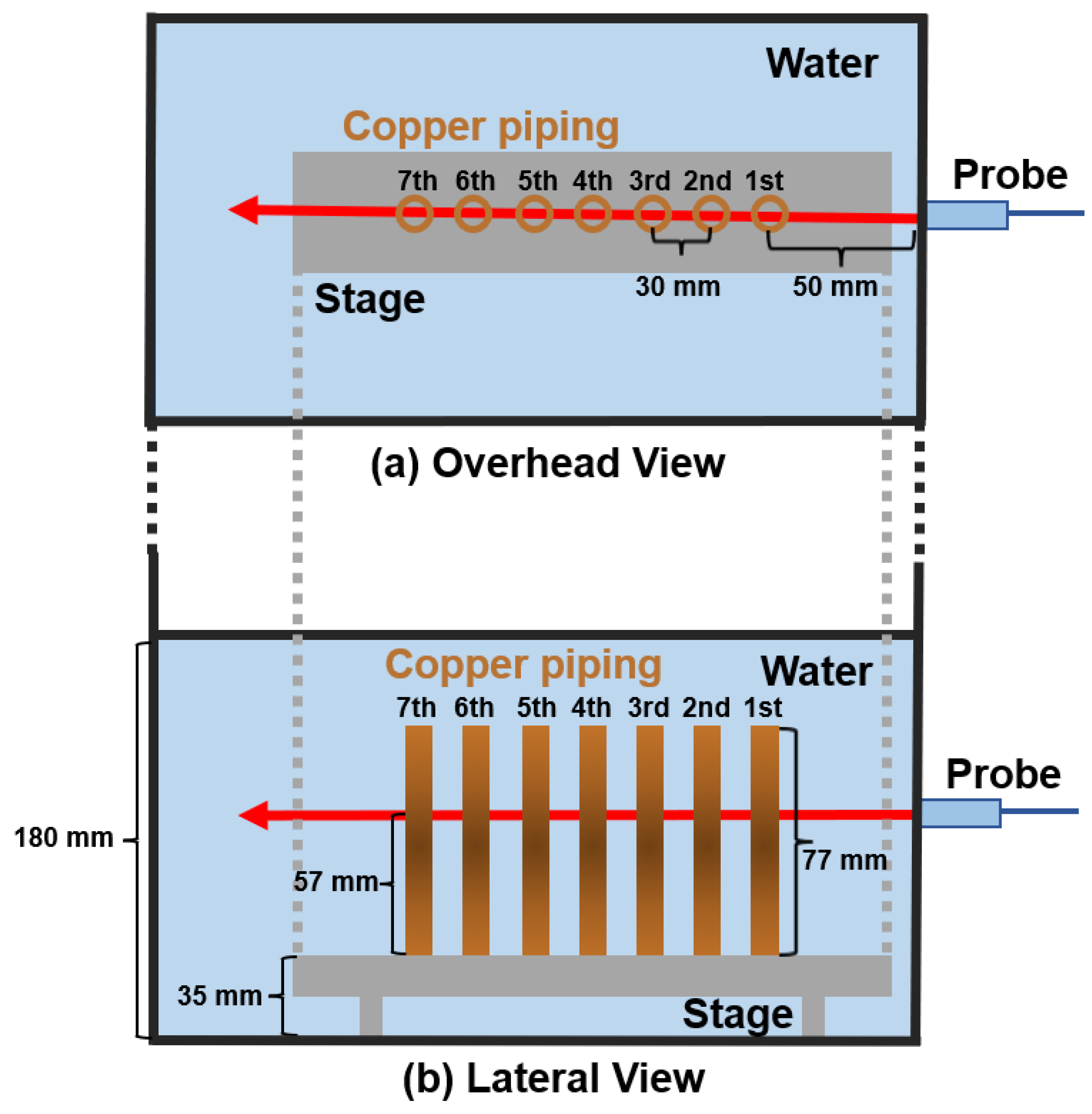
Figure 1. Schematic diagram of the experimental apparatus for bubble detection in water.
Applsci 15 12587 g001
Figure 2. The leakage direction of bubbles from each copper piping.
Applsci 15 12587 g002
Figure 3. Autoencoder model architecture.
Applsci 15 12587 g003
Figure 4. Phased-Array Images for Underwater Visualization. The “No Hole” label denotes the baseline condition, in which only the copper piping is present. The cardinal directions indicate the emission direction of the bubbles, all of which originate from the seventh copper pipe.
Applsci 15 12587 g004
Figure 5. Learning curve of CNN with EfficientNet-b0. Accuracy is defined as the ratio of correct predictions to the total number of samples. Loss is calculated using Cross-Entropy Loss.
Applsci 15 12587 g005
Figure 6. Visualization of the basis for classification using the Grad-CAM method. The results are averaged pixel-wise for individual heatmaps, calculated only from test data where the predicted label matched the actual label. The heatmap pixels align with those of the phased-array image, and the red regions correspond to the area most important to the CNN classification decision.
Applsci 15 12587 g006
Figure 7. t-SNE visualization of features for each class. (a) shows the result of applying t-SNE to the raw data of all 8400 experimental images. (b) shows the t-SNE visualization of the high-dimensional features. These features were obtained by feeding the output of the CNN model’s final fully connected layer.
Applsci 15 12587 g007
Figure 8. Reconstruction Error and Confusion Matrix in Autoencoder. (a) Reconstruction Error Distribution and Anomaly Detection Threshold. (b) Confusion Matrix for Anomaly Detection.
Applsci 15 12587 g008
Figure 9. LIME Visualization of Feature Importance for the seventh piping by the Autoencoder. The visualization was generated by analyzing only the data that the autoencoder correctly classified during anomaly detection, and averaging the feature importance maps from those individual results.
Applsci 15 12587 g009
Figure 10. Comparison of Original Experimental Images and Decoder-Reconstructed Images.
Applsci 15 12587 g010
Figure 11. Performance Evaluation of the One-Class SVM for Anomaly Detection. (a) Separation of Normal and Anomalous Data by Anomaly Scores. (b) Confusion Matrix for One Class SVM.
Applsci 15 12587 g011
Figure 12. LIME Visualization of criteria of classification for the “No Hole” Condition and 7th Copper Piping Bubble Generation.
Applsci 15 12587 g012
Figure 13. Comparison of Original and Reconstructed Images for Normal and 7th Pipe Anomalies.
Applsci 15 12587 g013
Figure 14. t-SNE visualization of per-class features. (a) t-SNE Visualization for the Autoencoder. (b) t-SNE Visualization for the OC-SVM utilizing latent features extracted by the Autoencoders. (c) t-SNE Visualization for the k-means utilizing latent features extracted by the Autoencoders. (d) t-SNE Visualization for the k-means utilizing latent features extracted by the Autoencoders trained with One Class SVM.
Applsci 15 12587 g014
Table 1. Acoustic Impedance Values for the Respective Materials [26,27,28].
Monju (325 °C) [MRayl]Monju (469 °C) [MRayl]This Study (25 °C) [MRayl]
Vessel44 (2.25Cr-1Mo steel)42 (2.25Cr-1Mo steel)46.32 (Type-304 Stainless steel)
Heat transfer tube44 (2.25Cr-1Mo steel)42 (2.25Cr-1Mo steel)42.65 (Copper)
Solvent2.1 (Sodium)1.9 (Sodium)1.49 (Water)
bubbles9.3 × 10−4 (Hydrogen)8.3 × 10⁻⁴ (Hydrogen)4.08 × 10⁻⁴ (Air)
Table 2. K-means Metrics Using Encoder Latent Features (Precision, Recall, F1-Score) per Class.
Copper Piping OrderBubbles DirectionPrecisionRecallF1-Score
-No Hole0.9560.9290.942
1stWest0.2150.7000.329
East0.000.000.00
North0.2560.5500.349
South0.000.000.00
2ndWest0.000.000.00
East0.1550.7500.256
North0.6820.7500.714
South0.2670.6000.369
3rdWest0.000.000.00
East0.09890.4500.162
North0.5630.4500.500
South0.000.000.00
4thWest0.4550.5000.476
East0.000.000.00
North0.000.000.00
South0.000.000.00
5thWest0.000.000.00
East0.000.000.00
North0.000.000.00
South0.000.000.00
6thWest0.000.000.00
East0.000.000.00
North0.000.000.00
South0.000.000.00
7thWest0.2350.9500.376
East0.000.000.00
North0.1740.7500.283
South0.000.000.00
Average0.1400.2540.164
Table 3. K-means Metrics (Precision, Recall, F1-Score) per Class on One Class SVM-Optimized Autoencoder Features.
Copper Piping OrderBubbles DirectionPrecisionRecallF1-Score
-No Hole0.9960.9680.982
1stWest0.5760.9500.717
East0.8260.9500.884
North1.000.9000.947
South0.6790.9500.792
2ndWest0.7830.9000.837
East0.3490.7500.476
North1.000.7500.857
South0.3140.5500.40
3rdWest0.000.000.00
East1.001.001.00
North0.9500.9500.950
South0.3870.600.471
4thWest0.9290.6500.765
East0.000.000.00
North0.5411.000.702
South0.000.000.00
5thWest0.6671.000.80
East0.4360.8500.576
North0.000.000.00
South0.000.000.00
6thWest1.001.001.00
East0.8701.000.930
North0.000.000.00
South0.000.000.00
7thWest0.8331.000.909
East0.000.000.00
North0.5131.000.678
South0.3771.000.548
Average0.5180.6450.559
Disclaimer/Publisher’s Note: The statements, opinions and data contained in all publications are solely those of the individual author(s) and contributor(s) and not of MDPI and/or the editor(s). MDPI and/or the editor(s) disclaim responsibility for any injury to people or property resulting from any ideas, methods, instructions or products referred to in the content.