Numerical Investigation of the Phase Change Behavior of Liquefied CO₂ in a Type-C Cryogenic Tank

Abstract

As global warming accelerates, the Paris Agreement has emphasized the urgent need for technologies that reduce and manage carbon dioxide emissions. Consequently, carbon capture and storage (CCS) has emerged as a critical area of research. For the safe and efficient transportation of captured carbon dioxide in cryogenic tanks, the design must accurately account for the phase change behavior of liquefied carbon dioxide (LCO₂). This study proposes a numerical approach to evaluate the thermal insulation performance of cryogenic tanks by simulating the phase change process of LCO₂. The phase transition of LCO₂ was simulated in a horizontally oriented Type-C cryogenic tank using the open-source computational fluid dynamics (CFD) framework OpenFOAM (v2312). To validate the numerical methodology, the phase change in liquefied nitrogen (LN₂) inside a tank was first simulated and compared with available experimental data. A mesh-independence study was then conducted to determine the optimal grid resolution, and the effects of different equations of state (EOS) for both liquid and gaseous phases, as well as various turbulence models, were examined. The boil-off rate (BOR) and boil-off gas (BOG) generation within the tank were predicted, and variations in internal pressure and flow fields were analyzed. The simulation results over 5000 s showed that the internal tank pressure increased from 7.8 bar to 8.1 bar, and the average temperature rose by approximately 1.3 K. The total mass of LCO₂ decreased from 1439.3 kg to 1431.0 kg.

1. Introduction

As global warming intensifies, reducing greenhouse gas emissions has become an urgent global priority [1,2]. To address this challenge, various direct mitigation approaches are being implemented, including improvements in energy efficiency and the adoption of eco-friendly fuels. However, to effectively manage the vast quantities of carbon dioxide emitted from everyday activities, power generation, and industrial processes, advanced technologies are essential. Consequently, the carbon dioxide capture, utilization, and storage (CCUS) has emerged as a key strategy for achieving substantial and sustainable reductions in greenhouse gas emissions [2,3].

The global effort to mitigate greenhouse gas emissions is embodied in the Paris Agreement, a landmark international treaty that aims to limit the rise in global average temperature to well below 2 °C above pre-industrial levels, and preferably to 1.5 °C [1]. Consequently, various industrial and energy sectors are striving to develop effective strategies for reducing and managing carbon dioxide emissions. A representative example is the maritime industry, which, through the International Maritime Organization (IMO), has adopted an initial strategy to drastically reduce greenhouse gas emissions by 2050 [4,5]. However, several analyses indicate that such ambitious targets are unlikely to be achieved solely through measures such as the adoption of eco-friendly fuels or improvements in ship efficiency using carbon dioxide emission-reduction technologies [4,5,6]. This finding underscores that emission reduction efforts at the source alone are insufficient to meet global climate goals, not only in the maritime sector but across all major industries. Therefore, carbon capture and storage (CCS) technology, which captures, stores, and transports carbon dioxide after its emission, is indispensable for achieving deep and sustained reductions in greenhouse gas emissions.

The successful implementation of CCS requires completion of the entire process chain, encompassing capture, transportation, and storage. In particular, large-scale CO₂ capture facilities and storage sites are often geographically separated [3]. Therefore, developing technologies capable of safely and economically transporting hundreds of millions of tons of CO₂ from capture locations to storage sites is of critical importance. Against this backdrop, maritime transport using liquefied carbon dioxide (LCO₂) carriers has emerged as one of the most practical and scalable solutions. However, LCO₂ poses significant technical challenges due to its cryogenic nature. Heat ingress from the external environment and sloshing motion induced by ship movement can cause vaporization of LCO₂ inside the tank, leading to potential safety hazards and economic losses. The typical operating pressure of LCO₂ tanks is reported to range from approximately 7 to 20 bar, depending on the saturation temperature and design conditions [7]. Consequently, accurate prediction of boil-off gas (BOG) and the boil-off ratio (BOR), which serve as key quantitative indicators for evaluating the thermal insulation performance of cryogenic storage tanks, is essential.

Numerous previous studies have investigated the storage and transportation of cryogenic fluids such as liquefied natural gas (LNG). Lin et al. [8] experimentally observed the phase change behavior of liquefied nitrogen (LN₂) in cryogenic tanks over time, providing valuable data for subsequent numerical analyses with an error of 3.82%. Wu and Ju [9] numerically analyzed boil-off gas (BOG) generation in a Type-C LNG tank subjected to sloshing motion using a two-phase volume of fluid (VOF) model that incorporated phase change and a dynamic mesh technique. The results verified that the relative error of the model was less than 5.0%. Jeon et al. [10] developed a high-fidelity multiphase thermal simulation approach that comprehensively accounts for heat transfer within the insulation system and phase change in the internal fluid, enabling accurate prediction of BOG and boil-off ratio (BOR) in LN₂ and LNG Type-C tanks. In a subsequent study, Jeon et al. [11] performed numerical analyses to estimate BOG generation from LN₂ in a vertical Type-C tank as a function of filling level, demonstrating high accuracy with errors within 3%. Jeong et al. [12] investigated BOG generation in cryogenic insulated tanks under sloshing conditions by simulating the motion of storage tanks installed on an actual vessel. The predicted BOG showed the errors within 7%.

In addition, numerous studies have investigated the storage and transportation of liquefied hydrogen (LH₂). Huerta and Vesovic [13] developed a new computational fluid dynamics (CFD) model capable of accurately predicting temperature and pressure in LH₂ and analyzed its evaporation behavior under non-isobaric conditions. Their analysis revealed that a substantial portion of the heat entering the gas phase under non-isobaric conditions was conducted along the tank walls, and this heat transfer pathway played a critical role in driving evaporation at the interfaces among the gas, liquid, and wall regions. Lv et al. [14] performed CFD simulations to examine the role of internal baffles in mitigating sloshing during long-distance transportation of large LH₂ tanks. While the baffles effectively suppressed sloshing, they also acted as thermal bridges under dynamic conditions, facilitating heat ingress into the tank and accelerating pressure rise. The pressure increase was particularly significant under strong sloshing conditions. Liu et al. [15] numerically analyzed sloshing phenomena in vertical LH₂ tanks using a CFD model that combined the VOF method with a dynamic mesh technique. Their study detailed free-surface fluctuations, the resulting forces and moments induced by sloshing, and variations in internal pressure with errors within 5%. Wei and Zhang [16] conducted a numerical investigation of the complex conditions that develop when sloshing occurs concurrently with the no-vent fill process of LH₂. They identified a critical regime in which weak sloshing suppressed pressure rise, whereas violent sloshing led to a rapid increase in internal pressure. Jeong et al. [17] developed a three-dimensional CFD model based on the VOF method to quantitatively evaluate the influence of polyurethane foam insulation thickness on the thermal performance of hydrogen storage tanks. Their results showed that increasing insulation thickness significantly reduced evaporative gas production, whereas internal supports caused flow stagnation and promoted localized liquid evaporation. Seo et al. [18] investigated the effects of tank inclination and filling level on BOG generation in LH₂ tanks through CFD simulations. They found that larger inclination angles amplified sloshing-induced vaporization, with the most pronounced BOG generation occurring at a 50% filling level.

For liquefied ammonia (LNH₃), Molkov et al. [19] simulated the entire process of liquid ammonia (LNH₃) release through a tank–piping–atmosphere system. They proposed a modified Lee phase change model [20] that dynamically adjusts the mass transfer rate. Yadav and Jeong [21] analyzed ammonia gas dispersion behavior during leakage incidents in a ship engine room by CFD. Overall, recent studies on LNH₃ have primarily focused on CFD simulations of emission and dispersion phenomena from storage tanks through connected pipeline systems.

Extensive research has been conducted on cryogenic fluids such as LNG, LN₂, and LH₂, including studies of phase-change prediction models based on experimental data and analyses of complex dynamic phenomena through numerical simulations. However, unlike other well-studied cryogenic fluids, LCO₂, a core component of carbon capture and storage (CCS) technology, exhibits relatively complex thermodynamic behavior. Most previous studies related to LCO₂ focus on pipe rupture, valve failure, and leakage [22]. As a result, research on the thermal insulation performance of LCO₂ storage tanks, boil-off gas (BOG) prediction, and sloshing characteristics remains at an early stage of development. Furthermore, most existing studies on LCO₂ rely heavily on commercial software, which restricts the flexibility to incorporate and validate diverse phase change models.

Therefore, this study developed a numerical methodology for analyzing the phase change behavior of LCO₂. Using the developed approach, the phase-change volume within an actual LCO₂ storage tank was predicted. Furthermore, the open-source CFD platform OpenFOAM (v2312) was employed and customized to implement the proposed analysis framework.

The remainder of this paper is organized as follows. The computational methodology and validation procedures are described first, followed by the presentation and discussion of the simulation results. Finally, the paper concludes with a summary of the key findings and a set of concluding remarks.

2. Computational Methods

2.1. Governing Equations

This study analyzed conjugate heat transfer and multiphase flow between the fluid and solid domains. The analysis was performed using the chtMultiRegionTwoPhaseEulerFoam solver from the open-source CFD library OpenFOAM (v2312). This solver employs an Eulerian–Eulerian two-fluid approach to model the fluid region [23]. For the solid region, it solves the heat conduction equation, enabling strong thermal coupling between the fluid and solid domains. In the two-fluid model, the liquid and gas phases are treated as interpenetrating continua that coexist in both space and time. Accordingly, the conservation equations for each phase are solved separately, and their interactions are represented through interphase transfer terms [24,25]. The governing equations used in this study are presented below.

The mass conservation equation for each phase k is expressed as a transport equation for the volume fraction (${\alpha }_k$) of that phase, incorporating the effects of interphase mass transfer due to phase change.

$${\displaystyle \frac{\partial ({\alpha }_k{\rho }_k)}{\partial t}}+\nabla ·({\alpha }_k{\rho }_k{u}_k)={\dot{m}}_k$$

(1)

Here, ${\rho }_k$ denotes the density of phase $k$, $U_k$ is the velocity vector of phase $k$, and ${\dot{m}}_k$ represents the interphase mass transfer rate per unit volume transferred to phase $k$ due to phase change. When the liquid temperature exceeds the saturation temperature, the excess energy is converted into mass transfer associated with phase change. This method is calculated from saturation pressure–temperature table data and can numerically reproduce evaporation and condensation processes in a physically consistent manner without empirical constants. In this study, $k$ corresponds to the liquid phase ($l$) and the gas phase ($g$). Accordingly, ${\dot{m}}_k$ represents the mass transfer between the two phases, satisfying the relationship ${\dot{m}}_l=-{\dot{m}}_g$. Additionally, the sum of the volume fractions of all phases satisfies the condition ${\alpha }_l+{\alpha }_g=1$.

The momentum conservation equation for each phase $k$ ($k=l,g$) is expressed as follows:

$${\displaystyle \frac{\partial ({\alpha }_k{\rho }_k{U}_k)}{\partial t}}+\nabla ·({\alpha }_k{\rho }_k{U}_k{U}_k)=-{\alpha }_k\nabla p+\nabla ·({\alpha }_k{\tau }_k)+{\alpha }_k{\rho }_{k}g+M_k$$

(2)

Here, $p$ denotes the pressure shared by both phases, ${\tau }_k$ is the stress tensor that includes viscous and turbulent stresses, and g is the gravitational acceleration vector. $M_k$ represents the interphase momentum transfer term, accounting for effects of interfacial interactions such as drag, lift, and turbulent dispersion forces.

In the fluid domain, the energy conservation for each phase $k$ is expressed as a transport equation for the enthalpy ($h_k$):

$${\displaystyle \frac{\partial ({\alpha }_k{\rho }_k{h}_k)}{\partial t}}+\nabla ·({\alpha }_k{\rho }_k{U}_k{h}_k)={\alpha }_k{\displaystyle \frac{Dp}{Dt}}+\nabla ·({\alpha }_k{k}_{eff,k}\nabla T_k)+Q$$

(3)

Here, $k_{eff,k}$ is the effective thermal conductivity, $T_k$ is the temperature, and $Q$ is the interphase energy exchange term, which includes latent heat associated with interphase heat transfer and phase change.

To analyze the thermo-fluid behavior inside the LCO₂ storage tank, both the ideal gas law and the Peng–Robinson equation of state (PR-EOS) were considered. The ideal gas law is the most classical form of an EOS and accurately describes the behavior of real gases under low-pressure and high-temperature conditions. It is expressed as follows:

$$p{v}_m=RT$$

(4)

Here, $v_m$ is the molar volume, $T$ is the temperature, and $R$ is the universal gas constant, with a value of 8.31451 $\mathrm{J}·{\mathrm{m}\mathrm{o}\mathrm{l}}^{-1}{\mathrm{K}}^{-1}$ [26].

The PR-EOS is a cubic EOS derived from the van der Waals approach, which describes the thermodynamic behavior of real gases. It incorporates two parameters, $a$ and $b$, representing the intermolecular attractive and repulsive forces, respectively. The equation is expressed as follows:

$$p={\displaystyle \frac{RT}{v_m-b}}-{\displaystyle \frac{a(T)}{{v_m}^2+2b{v}_m-b^2}}$$

(5)

where

$$a(T)=0.45724{\displaystyle \frac{R^2{T_c}^2}{P_c}}·{[1+\kappa (1-{T_r}^{1/2})}^2$$

(6)

$$b=0.0778{\displaystyle \frac{R{T}_c}{P_c}}$$

(7)

In this equation, $T_c$ and $P_c$ denote the critical temperature and critical pressure, respectively, while $T_r$ represents the reduced temperature (${T/T}_c$). Here, $T_c$ = 304.13 K and $P_c$ = 7.3773 MPa were used. The parameter $\kappa$ is an empirical coefficient related to the acentric factor, which quantifies the degree to which a molecule’s shape deviates from ideal spherical symmetry. $k$ is defined as $k=0.37464+1.54226\omega -0.26992{\omega }^2$, where $\omega$ is 0.2249 [27]. A key advantage of the PR-EOS is that it can be expressed as a cubic polynomial in molar volume, allowing for direct analytical solutions and enabling highly efficient computational performance. The PR-EOS may exhibit somewhat lower accuracy in regions near critical points, where density changes are abrupt. However, the Span–Wagner EOS [28] demonstrates higher reliability in such regions. It also has the disadvantage of being computationally very expensive. Therefore, to balance computational efficiency and the reproducibility of thermophysical properties, this study adopted the PR-EOS for numerical analysis.

To accurately model the momentum exchange between the two phases, several interfacial forces were considered. The drag force, which primarily governs bubble dynamics, was modeled using the Ishii–Zuber correlation [29], while the lift force, responsible for inducing lateral bubble motion, was represented by the Tomiyama model [30]. In addition, the wall lubrication force, which acts to repel bubbles from the wall region, the virtual mass force associated with bubble acceleration, and the turbulent dispersion force arising from turbulence were also incorporated. These considerations enabled a physically realistic prediction of bubble trajectories and spatial distributions within the flow domain.

To simulate the phase change process, an evaporation model was employed in which phase transition occurs when the liquid temperature reaches the saturation temperature corresponding to the local pressure. The saturation temperature is dynamically computed as a function of pressure by referencing external tabulated data [31] containing the corresponding saturation pressure–temperature pairs. To achieve numerical stability, under-relaxation was applied when calculating the latent heat term in the energy equation.

The interfacial heat transfer between a bubble and the surrounding liquid was evaluated using the Ranz–Marshall correlation [32], which assumes a spherical bubble to determine the Nusselt number ($Nu$). This model requires the Prandtl number ($Pr$), a dimensionless parameter representing the ratio of momentum diffusivity to thermal diffusivity. In the present simulation, this correlation was applied to both the gas and liquid phases [33]. The correlation is expressed as follows:

$$Nu=2+0.6{Re}_{slip}^{0.5}{Pr}^{0.3}$$

(8)

where

$${Re}_{slip}={\displaystyle \frac{V_{slip}{d}_v}{v_l}}$$

(9)

$$\mathit{Pr}={\displaystyle \frac{{\mu }_l·c_p}{k_l}}$$

(10)

Here, ${Re}_{slip}$ denotes the slip velocity Reynolds number, $V_{slip}$ denotes the slip velocity between the liquid and vapor phases, ${\mu }_l$ is the dynamic viscosity of the liquid phase, and $c_p$ is the specific heat capacity. In OpenFOAM (v2312), when the thermophysical properties of each fluid, namely the kinematic viscosity, specific heat capacity, and thermal conductivity, are specified as input parameters, the Prandtl number is internally computed from these quantities and subsequently used in the heat transfer analysis. The combination of the detailed physical models described above enables a more comprehensive and physically consistent analysis of BOG generation and behavior compared with previous studies.

The mixture $k-\epsilon$ turbulence model was employed to account for turbulent flow within the LCO₂ storage tank [34]. This model is formulated for two-phase (gas–liquid) mixtures. To represent the influence of bubble motion on the surrounding flow, additional source terms $S_k$ and $S_{\epsilon }$ [35], were incorporated into the standard $k-\epsilon$ equations. These terms primarily model the generation of turbulent kinetic energy resulting from interphase drag between the liquid and gas phases.

In the solid regions, such as the insulation layer, heat transfer was modeled using the classical heat conduction equation [36].

$${\rho }_s{c}_{p,s}{\displaystyle \frac{\partial T_s}{\partial t}}=\nabla ·(k_s\nabla T_s)$$

(11)

Here, ${\rho }_s$ denotes the solid density, $c_{p,s}$ represents the specific heat capacity of the solid at constant pressure, and $k_s$ is the thermal conductivity of the solid. At the fluid–solid interface, the energy equations for the two domains are coupled through the continuity conditions of temperature and heat flux.

2.2. Thermophysical Properties

The saturation curves, enthalpy, specific heat capacity, and other key thermophysical properties of LN₂ and LCO₂ were obtained from the CoolProp library [31]. The backend used is Helmholtz EOS (HEOS), and CoolProp (v6.6.0) was used. CoolProp (v6.6.0) is an open-source thermophysical property library that provides accurate data for 122 pure and quasi-pure fluids. Using a high-precision EOS based on the Helmholtz free energy, the library enables consistent calculations of various thermodynamic and transport properties, such as pressure, density, enthalpy, and entropy, over a wide range of temperatures and pressures [37]. Unlike simplified correlations or limited tabulated datasets, CoolProp (v6.6.0) ensures flexibility, reproducibility, and thermodynamic consistency among property values. These features allow for a more accurate representation of real fluid behavior in CFD analyses of cryogenic storage tanks.

2.3. Numerical Methods

A pressure-based, cell-centered, finite-volume method was employed together with a linear reconstruction scheme that accommodates computational cells of arbitrary shapes. Time derivative terms were discretized using a first-order implicit Euler scheme, which provides sufficient engineering accuracy when an appropriately small time step is selected. Solution gradients at the cell centers were evaluated using the Gauss linear scheme. The convection terms were discretized with a limited linear upwind interpolation scheme with the blending factor of 1.0, while diffusion terms were treated using the Gauss linear corrected scheme. Velocity–pressure coupling and the overall solution procedure were implemented through a hybrid algorithm that combines the Semi-Implicit Method for Pressure-Linked Equations (SIMPLE) and the Pressure-Implicit with Splitting of Operators (PISO) method, adapted for unstructured grids. The van Leer scheme was applied for interface capturing between the two phases. The resulting discretized algebraic equations were solved using a point-wise Gauss–Seidel iterative method, and an algebraic multigrid (AMG) approach was employed to accelerate convergence.

3. Validation for an LN₂ Tank

To validate the numerical methods, the phase change behavior in an LN₂ storage tank was analyzed. A type-C cryogenic tank, as illustrated in Figure 1, was considered for this validation [8]. The tank consists of an outer shell, an inner tank, and an insulation layer positioned between them. The insulation space separating the outer and inner tanks was modeled as a solid domain, whereas the interior of the inner tank was modeled as a fluid domain.

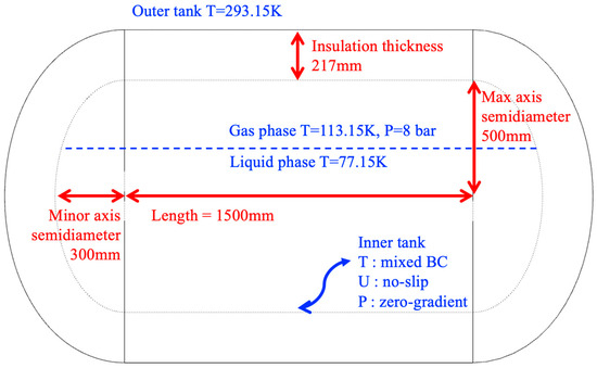
Figure 1. Geometric configuration and dimensions of the LN₂ tank.

The geometric dimensions are shown in Figure 1. The total length of the tank is 1500 mm, and the insulation thickness is 400 mm.

The LN₂ tank consists of an inner tank and an outer tank. The outer tank is exposed to the external environment. Therefore, a fixed wall temperature of 293.15 K was applied to represent ambient atmospheric conditions, and convective heat transfer with the surroundings was neglected. If a high ambient temperature is specified as the ambient atmospheric condition, the phase change is expected to occur more rapidly. The inner tank includes two boundary surfaces, one in contact with the fluid domain and the other with the solid insulation domain, necessitating thermal coupling between these interfaces. A mixed boundary condition accounting for temperature and radiative heat transfer was applied to the tank surface in contact with the fluid domain. The initial wall temperatures were set to 113.15 K for the gas phase and 77.15 K for the liquid phase. A no-slip condition was imposed on velocity at all solid boundaries. For pressure, a zero gradient boundary condition was applied, with an initial internal pressure of 1 bar. At the interface between the solid domain and the inner tank, the same temperature coupling condition was imposed to account for conductive heat transfer between the insulation and the fluid domain.

To evaluate the thermal insulation performance through CFD analysis, experimental data [8] were used to verify the accuracy of the numerical simulation. The cryogenic fluid contained within the tank was LN₂, and boil-off gas generation was compared at a 60% filling level condition. The thermophysical properties of LN₂ and nitrogen (N₂) were set as listed in Table 1. The initial fluid temperatures were assigned as 77.15 K for the liquid phase and 113.15 K for the gaseous phase, consistent with the experimental conditions [8] and summarized in Table 2. The thermophysical properties of the solid insulation region were defined as given in Table 3. The properties of the insulation material are largely unaffected by temperature; thus, constant values were used.

Table 1. Thermophysical properties of LN₂ and N₂.

	Enthalpy of Vaporization [kJ/kg]	Density [kg/m3]	Specific Heat [J/kg·K]	Conductivity [W/(m·K)]
LN2	198.6	808.3	-	-
N2	-	1.25	1038	0.009

Table 2. Initial temperature of LN₂ and N₂.

	LN2	N2
Temperature [K]	77.15	113.15

Table 3. Thermophysical properties of insulation material.

Conductivity [W/(m·K)]	Specific Heat [J/kg·K]	Density [kg/m3]
0.023	29	45

A mesh-convergence test was conducted to evaluate the influence of mesh resolution on phase change behavior. Figure 2 illustrates the configurations of the coarse, medium, and fine meshes used in this test, consisting of approximately 200,000, 400,000, and 600,000 grid points, respectively. A locally refined mesh was applied near the gas–liquid interface (free surface) in all cases to ensure numerical stability and accuracy in simulating phase change phenomena. The simulations were executed on a 70-core Intel^® Xeon^® Platinum 8558 CPU (4.0 GHz). The total computational time ranged from approximately 2 to 10 days, depending on the mesh resolution. The time step was dynamically adjusted during the computations to ensure the Courant number (Co) remained below 1. This approach secured numerical stability while enabling precise capture of the transient phase change

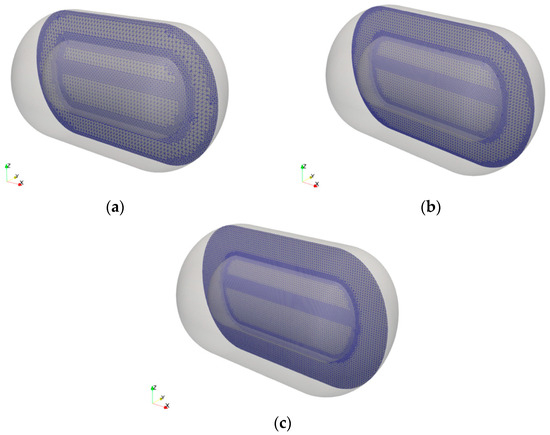
Figure 2. Three levels of mesh resolution used for the validation: (a) coarse mesh; (b) medium mesh; (c) fine mesh.

Figure 3 presents the temperature contours inside the tank over time, obtained using the medium mesh. As time progresses, heat ingress from the ambient atmosphere is conducted through the insulation (solid region) and subsequently transferred to the inner tank wall. Consequently, phase change occurs progressively near the fluid–solid boundary, indicating an increasing transition from the liquid phase to the vapor phase over time.

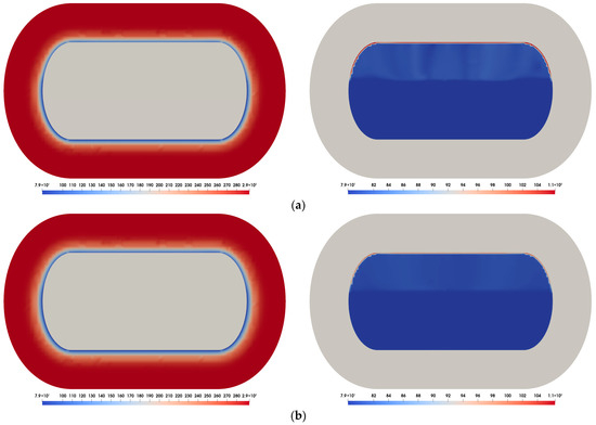
Figure 3. Temperature contours inside the LN₂ tank: (a) $t$ = 100 s ((left): insulation, (right): inner tank); (b) $t$ = 5000 s ((left): insulation, (right): inner tank).

Figure 4 presents the variation in BOG generation with different mesh resolutions. BOG ($m_{BOG}$) was defined as the product of the liquid density and the volume of evaporated liquid over time. BOG indicates the cumulative evaporated mass and is expressed as follows:

$$m_{BOG}[kg]={\rho }_{liquid}[V_0-V\left(t\right)]$$

(12)

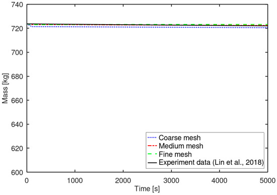
Figure 4. BOG generation under different mesh resolutions [8].

Here $V_0$ and $V\left(t\right)$ indicate the initial volume and volume at a certain time of the liquid phase. Taking the derivative of BOG with respect to time yields the BOG rate (${\dot{m}}_{BOG}$), expressed as follows:

$${\dot{m}}_{BOG}[\mathrm{k}\mathrm{g}/\mathrm{s}]={\rho }_{liq}{\displaystyle \frac{d(V_0-V\left(t\right))}{dt}}$$

(13)

The coarse mesh tended to overpredict the phase change rate, whereas the medium and fine meshes accurately captured the phase change behavior, showing good agreement with the experimental results [8]. The difference between the calculated BOG using the three meshes and the experimental data was less than 0.15% in all cases. The selected numerical methods were confirmed to reproduce the phase change behavior with high accuracy. Based on the analysis of the LN₂ tank results, the medium mesh was selected for subsequent phase change simulations of the LCO₂ tank.

4. Results and Discussion

The phase-change behavior of LCO₂ in a Type-C cryogenic tank was analyzed. The numerical methodology applied in this analysis was identical to that used in the LN₂ validation case. Figure 5 illustrates the configuration of the Type-C cryogenic tank, which is generally similar to that of the LN₂ tank. The overall tank length is 1500 mm, and the insulation thickness is 217 mm.

Figure 5. Geometric configuration, dimensions, and boundary conditions of the vLCO₂ tank.

Figure 6 shows the mesh configuration used in the insulation and Inner tank regions. The same mesh resolution as the medium mesh employed in the LN₂ mesh convergence test was adopted. The total number of meshes used was 213,211 for the fluid domain and 203,025 for the solid insulation domain.

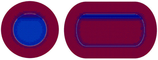
Figure 6. Initial filling level of LCO₂ in the tank (94.5%).

The LCO₂ tank consists of an inner tank and an outer tank, identical in configuration to the LN₂ tank. The outer tank is exposed to the external environment. Therefore, a fixed wall temperature of 293.15 K was imposed to represent ambient atmospheric conditions, and convective heat transfer with the surroundings was neglected. The inner tank has two interfaces: one with the fluid domain and the other with the solid insulation domain, necessitating thermal coupling between them. A mixed boundary condition for temperature and radiative heat transfer was applied to the tank surface in contact with the fluid domain. The initial wall temperatures were set to 234.25 K for the gas phase and 227.05 K for the liquid phase. A no-slip condition was imposed for velocity at all solid boundaries, while a zero gradient boundary condition was applied for pressure with an initial value of 7.8 bar. At the interface between the solid domain and the inner tank, the same temperature coupling condition was enforced to account for conductive heat transfer between the insulation and the fluid domain.

Figure 6 illustrates the initial filling condition of LCO₂ inside the tank. An initial filling ratio of 94.5% was adopted. A locally refined mesh was generated near the liquid–gas interface to accurately capture interfacial phenomena. The initial conditions specified a temperature of 234.25 K for the gaseous carbon dioxide, 227.05 K for the LCO₂, and an initial internal pressure of 7.8 bar. The time step was chosen such that the Courant number ($Co$) remained below 1 throughout the computation to ensure numerical stability.

For carbon dioxide, research has been less extensive than for cryogenic fluids such as LN₂ or LNG. Therefore, comparative analyses were conducted to identify the most suitable turbulence models and equations of state (EOS) for simulating LCO₂.

The turbulence models considered included the widely used standard $k-\epsilon$ model, the shear stress transport (SST) $k-\omega$ model, and the mixture $k-\epsilon$ model [34], which is known for its advantages in modeling idealized multiphase flows. Figure 7 presents the phase contours and interface obtained with the different turbulence models. Results from the standard $k-\epsilon$ model exhibited excessive prediction of free surface ripples, whereas the mixture $k-\epsilon$ and SST $k-\omega$ models produced stable free surfaces without such oscillations. However, during wave–structure interaction simulations, the SST $k-\omega$ model was found to cause excessive smearing of the free surface [38]. Consequently, the mixture $k-\epsilon$ model was selected as the turbulence model for this study.

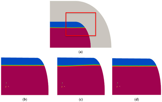
Figure 7. Free surface shape obtained using different turbulence models: (a) region of interest; (b) mixture $k-\epsilon$ model; (c) standard $k-\epsilon$ model; (d) SST $k-\omega$ model.

The influence of different equations of state (EOS) on the phase transition of carbon dioxide was investigated. Böttcher [27] compared numerical results obtained using four EOS models: ideal gas [39], Peng–Robinson [40], Duan–Müller–Weare [41], and Span–Wagner [28], against experimental thermophysical property data for CO₂. The results demonstrated that the Span–Wagner and PR-EOS provided the most accurate representation of real fluid behavior [28,40]. From a numerical convergence perspective, the ideal gas law exhibited superior stability during the simulation. Accordingly, the present study focused on comparing two EOS models: the ideal gas law and the PR-EOS [39,40], with the objective of improving the accuracy of CO₂ phase transition prediction.

Figure 8 presents the temperature contours of carbon dioxide as predicted using the different equations of state. Heat ingress from the ambient atmosphere is conducted through the insulation (solid region) and subsequently transferred to the inner tank wall. As time progresses, the carbon dioxide becomes increasingly affected by this heat transfer, resulting in phase change near the fluid–solid interface. Overall, the temperature distribution shows only minor variations among the different equations of state models.

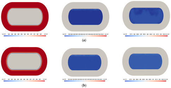
Figure 8. Temperature contours inside the LCO₂ tank: (a) $t$ = 100 s ((left): insulation; (center): inner tank with perfect gas EOS [39]; (right): inner tank with PR-EOS [40]); (b) $t$= 5000 s ((left): insulation; (center): inner tank with perfect gas EOS [39]; (right): inner tank with PR-EOS [40]).

Figure 9 shows the variation in BOG generation with different EOSs. The temporal evolution of BOG indicates that it remains nearly identical across the EOS models, although the perfect gas EOS gradually predicts a higher degree of phase change over time. This difference arises because the PR-EOS accounts for intermolecular interactions and the actual compressibility of the gas. Consequently, compared to the ideal gas law, the onset of vaporization is somewhat delayed, and the predicted vaporization volume is relatively smaller [27]. After 5000 s, the perfect gas EOS predicted approximately 0.4 kg (about 0.03%) more evaporation than the PR-EOS. Pressure distributions were monitored over time at one probe located in the gas phase and four probes positioned in the liquid phase. Figure 10 presents the temporal variation in pressure at each probe position, obtained using the PR-EOS [40]. The results clearly show an overall pressure increase inside the tank at all locations as boil-off gas generation progressed. The pressure measured at the gas phase probe (Probe 1) was lower than that at the liquid phase probes, reflecting the additional hydrostatic pressure contribution from the underlying liquid column. External heat is conducted through the outer tank and insulation into the inner tank. LCO₂ adjacent to the inner tank absorbs heat, causing localized evaporation. Evaporation at the liquid–gas interface generates BOG, increasing the gas-phase volume while decreasing the liquid volume. This also increases the pressure inside the tank.

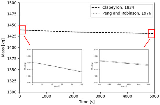
Figure 9. BOG generation predicted using different equations of state [39,40].

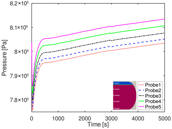
Figure 10. Pressure distribution inside the LCO₂ tank calculated using the PR-EOS [40].

The temporal variation in temperature inside the tank was analyzed to investigate the heat transfer characteristics of both phases. Figure 11 shows the probe locations used for temperature measurements in the liquid and gas regions. For the liquid phase, three probe points (Probe4(0, 0, 0.35), Probe5(−0.4, 0, 0.0), Probe6(−0.8, 0, −0.35)) were positioned linearly between the center of the initial liquid–gas interface and the inner tank wall. Similarly, for the gas phase, three probe points (Probe1(−0.8, 0, 0.48), Probe2(−0.4, 0, 0.44), Probe3(0, 0, 0.40)) were arranged linearly between the inner tank wall and the region immediately below the interface. Figure 12 presents the temperature distributions recorded at each probe location. The temperature profiles exhibited an approximately linear distribution in both the liquid and gas phases. Temperatures were generally higher near the wall than at interior locations. The temperature by PR-EOS differs from that by perfect gas EOS because it accounts for real gas behavior. The PR-EOS, which incorporates compressibility, influenced the temperature [27]. As the distance from the wall increased, the temperature decreased while maintaining a nearly constant spatial gradient. The temperature variations observed at different probe locations within the tank showed the same trend as those reported for the hydrogen tank [42].

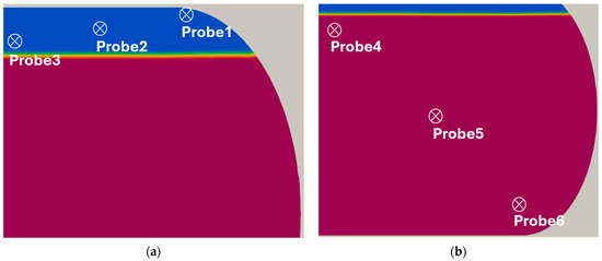
Figure 11. Probe locations: (a) probes at the gas phase; (b) probes at the liquid phase.

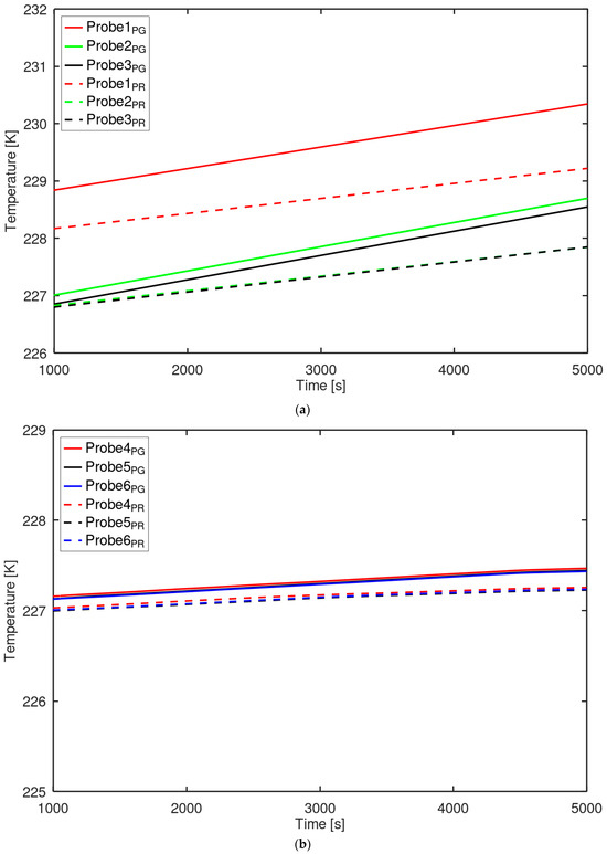
Figure 12. Temperature variation at probe locations: (a) gas phase; (b) liquid phase.

The heat ingression and evaporation inside the tank induce natural convection. In particular, the gas phase, having a lower density than the liquid phase, exhibits stronger convective motion, making convection the dominant transport mechanism. To visualize this behavior, streamlines in the gas phase were visualized based on the local velocity field. Figure 13 presents the streamlines, with the color distribution indicating the magnitude of the velocity. Flow is observed to rise near the tank wall and descend near the center. When heat conducted from the exterior wall is transferred to CO₂ near the inner tank wall, local superheating occurs. This results in an increase in vaporization due to the external heat influx.

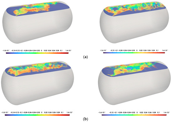
Figure 13. Streamlines in the gas phase: (a) $t$ = 1000 s ((Left): Clapeyron [39], (Right): PR-EOS [40]); (b) t = 5000 s ((Left): Clapeyron [39], (Right): PR-EOS [40]).

5. Concluding Remarks

To establish and validate the numerical methodology, verification computations were first conducted using experimental data from LN₂ phase-change tests. A mesh convergence analysis was performed with three different mesh resolutions, confirming that the predicted boil-off gas (BOG) generation asymptotically approached the experimental results as the mesh density increased. Among the tested meshes, the medium resolution mesh demonstrated accuracy comparable to that of the fine mesh while reducing computational time by more than half, thereby providing the optimal balance between accuracy and efficiency.

The verified numerical analysis techniques were applied to an LCO₂ tank to investigate the effects of turbulence model and EOS on phase change behavior. The Standard $k-ϵ$ model exhibited instability due to fluctuations at the liquid–gas interface, whereas the Mixture $k-ϵ$ model and SST $k-\omega$ model provided stable computations at the interface. To examine the influence of the EOS on phase change, the ideal gas law and the PR-EOS [40] were employed. The BOG generation, as well as temperature and pressure distributions, were compared at various locations inside the tank. While the BOG generation predicted by the different EOS models was nearly identical, the overall pressure evolution exhibited distinct patterns. Additionally, the fluid flow induced by natural convection in the gas phase was visualized to elucidate the internal heat- and mass-transfer characteristics. The findings of this research are expected to improve the reliability and predictive capability of future LCO₂ storage and transportation system designs.

This paper does not directly compare the present results with experiments on LCO₂ tanks. As future research, phase change experiments on LCO₂ tanks will be performed and compared with the present results.

References

- United Nations Framework Convention on Climate Change (UNFCCC). Paris Agreement; UNFCCC: Paris, France, 2015; Available online: https://unfccc.int/process-and-meetings/the-paris-agreement (accessed on 5 November 2025).
- International Energy Agency (IEA). Carbon Capture, Utilisation and Storage (CCUS): The Critical Technology for Net Zero Emissions; IEA: Paris, France, 2023; Available online: https://www.iea.org/energy-system/carbon-capture-utilisation-and-storage (accessed on 5 November 2025).
- Global CCS Institute. Global Status of CCS 2023; Global CCS Institute: Melbourne, Australia, 2023. [Google Scholar]
- Abioye, O.F.; Mohd Zaki, N.I.; Yusuf, N.; Mohd Yusop, M.Z.; Mohd Zaki, S.H. Technical Requirements for 2023 IMO GHG Strategy. Sustainability 2024, 16, 2766. [Google Scholar] [CrossRef]
- Mok, Y.S.; Kim, H.J.; Lee, S.H. The Integration of Carbon Capture, Utilization, and Storage (CCUS) in Waste-to-Energy Plants: A Review. Energies 2025, 18, 1883. [Google Scholar] [CrossRef]
- Joung, T.H.; Kang, S.G.; Lee, J.K.; Ahn, J. The IMO initial strategy for reducing greenhouse gas (GHG) emissions, and its follow-up actions towards 2050. J. Int. Marit. Saf. Environ. Aff. Shipp. 2020, 4, 1–7. [Google Scholar] [CrossRef]
- DNV. CO2 Transport—Recommended Practice DNV-RP-F104; DNV: Høvik, Norway, 2023; Available online: https://www.dnv.com (accessed on 5 November 2025).
- Lin, Y.; Ye, C.; Yu, Y.Y.; Bi, S.W. An approach to estimating the boil-off rate of LNG in type C independent tank for floating storage and regasification unit under different filling ratio. Appl. Therm. Eng. 2018, 135, 463–471. [Google Scholar] [CrossRef]
- Wu, S.; Ju, Y. Numerical study of the boil-off gas (BOG) generation characteristics in a type C independent liquefied natural gas (LNG) tank under sloshing excitation. Energy 2021, 223, 120001. [Google Scholar] [CrossRef]
- Jeon, G.M.; Park, J.C.; Choi, S.G. Multiphase-thermal simulation on BOG/BOR estimation due to phase change in cryogenic liquid storage tanks. Appl. Therm. Eng. 2021, 184, 116264. [Google Scholar] [CrossRef]
- Jeon, G.M.; Park, J.C.; Kim, J.W.; Lee, Y.B.; Kim, D.S.; Kang, D.E.; Lee, S.B.; Lee, S.W.; Ryu, M.C. Experimental and numerical investigation of change in boil-off gas and thermodynamic characteristics according to filling ratio in a C-type cryogenic liquid fuel tank. Energy 2022, 255, 124530. [Google Scholar] [CrossRef]
- Jeong, S.M.; Jeon, G.M.; Park, J.C.; Park, S. Sloshing effect on BOG/BOR in cryogenic liquid storage tank using multiphase-thermal simulations. In Proceedings of the ISOPE International Ocean and Polar Engineering Conference, Rhodes, Greece, 16–21 June 2024. [Google Scholar]
- Huerta, F.; Vesovic, V. CFD modelling of the non-isobaric evaporation of cryogenic liquids in storage tanks. Appl. Energy 2024, 356, 124240. [Google Scholar] [CrossRef]
- Lv, H.; Chen, L.; Zhang, Z.; Chen, S.; Hou, Y. Numerical study on thermodynamic characteristics of large-scale liquid hydrogen tank with baffles under sloshing conditions. Int. J. Hydrog. Energy 2024, 57, 562–574. [Google Scholar] [CrossRef]
- Liu, Z.; Feng, Y.; Lei, G.; Li, Y. Fluid sloshing dynamic performance in a liquid hydrogen tank. Int. J. Hydrogen Energy 2019, 44, 13885–13894. [Google Scholar] [CrossRef]
- Wei, G.; Zhang, J. Numerical study of the filling process of a liquid hydrogen storage tank under different sloshing conditions. Processes 2020, 8, 1020. [Google Scholar] [CrossRef]
- Jeong, S.-J.; Lee, S.-J.; Moon, S.-J. CFD thermo-hydraulic evaluation of a liquid hydrogen storage tank with different insulation thickness in a small-scale hydrogen liquefier. Fluids 2023, 8, 239. [Google Scholar] [CrossRef]
- Seo, Y.M.; Noh, H.W.; Hwang, D.W.; Koo, R.K. Numerical study on the effects of gravity direction and hydrogen filling rate on BOG in the liquefied hydrogen storage tank. J. Hydrog. New Energy 2023, 34, 342–349. [Google Scholar] [CrossRef]
- Molkov, V.; Sivaraman, S.; Cirrone, D.; Truchot, B.; Makarov, D. Modelling and numerical simulations of heat and mass transfer in multiphase flow during the release of liquid ammonia from a storage tank through the piping system to the open atmosphere. Int. J. Heat Mass Transf. 2025, 246, 127097. [Google Scholar] [CrossRef]
- Lee, W.H. A Pressure Iteration Scheme for Two-Phase Flow Modeling; Los Alamos National Laboratory: Los Alamos, NM, USA, 1979. [Google Scholar]
- Yadav, A.; Jeong, B. Safety evaluation of using ammonia as marine fuel by analysing gas dispersion in a ship engine room using CFD. J. Int. Marit. Saf. Environ. Aff. Shipp. 2022, 6, 99–116. [Google Scholar] [CrossRef]
- Liang, Y.; Kurokawa, Y.; Sato, T. Safety Assessment of Pressure Relief Valve Failure in Liquefied CO2 Storage Systems under Transient Overpressure Conditions. J. Loss Prev. Process Ind. 2024, 87, 105348. [Google Scholar] [CrossRef]
- Lian, J.; Yang, X.; Ma, B.; Gou, W. A novel method for bounding the phase fractions at both ends in Eulerian multi-fluid model. Comput. Fluids 2022, 243, 105512. [Google Scholar] [CrossRef]
- Rusche, H. Computational Fluid Dynamics of Dispersed Two-Phase Flows at High Phase Fractions. Ph.D. Thesis, Imperial College London, London, UK, 2002. [Google Scholar]
- Brazhenko, V.; Qiu, Y.; Cai, J.; Wang, D. Thermal evaluation of multilayer wall with a hat-stringer in aircraft design. J. Mech. Eng. 2022, 68, 635–641. [Google Scholar] [CrossRef]
- Cohen, E.R.; Taylor, B.N. The 1986 adjustment of the fundamental physical constants. Rev. Mod. Phys. 1986, 59, 1121. [Google Scholar] [CrossRef]
- Böttcher, N.; Taron, J.; Kolditz, O.; Liedl, R.; Park, C.-H. Comparison of equations of state for carbon dioxide for numerical simulations. In Proceedings of the International Conference on Heat Transfer and Fluid Flow, Prague, Czech Republic, 11–12 August 2014. [Google Scholar]
- Span, R.; Wagner, W. A new equation of state for carbon dioxide covering the fluid region from the triple-point temperature to 1100 K at pressures up to 800 MPa. J. Phys. Chem. Ref. Data 1996, 25, 1509–1596. [Google Scholar] [CrossRef]
- Ishii, M.; Zuber, N. Drag coefficient and relative velocity in bubbly, droplet and particulate flows. AIChE J. 1979, 25, 843–855. [Google Scholar] [CrossRef]
- Tomiyama, A.; Tamai, H.; Zun, I.; Hosokawa, S. Transverse migration of single bubbles in simple shear flows. Chem. Eng. Sci. 2002, 57, 1849–1858. [Google Scholar] [CrossRef]
- CoolProp. Available online: https://coolprop.org (accessed on 16 October 2025).
- Ranz, W.E.; Marshall, W.R. Evaporation from drops. Chem. Eng. Prog. 1952, 48, 141–146. [Google Scholar]
- Höhne, T.; Krepper, E.; Montoya, G.; Lucas, D. CFD-simulation of boiling in a heated pipe including flow pattern transitions using the GENTOP concept. Nucl. Eng. Des. 2017, 322, 165–176. [Google Scholar] [CrossRef]
- Behzadi, A.; Issa, R.I.; Rusche, H. Modelling of dispersed bubble and droplet flow at high phase fractions. Chem. Eng. Sci. 2004, 59, 759–770. [Google Scholar] [CrossRef]
- Lahey, R.T., Jr. The simulation of multidimensional multiphase flows. Nucl. Eng. Des. 2005, 235, 1043–1060. [Google Scholar] [CrossRef]
- Mulemane, A.; Murthy, J.Y.; Mathur, S.R. Conjugate heat transfer simulations using unstructured finite-volume discretization. Numer. Heat Transf. Part B Fundam. 2007, 51, 535–556. [Google Scholar]
- Bell, I.H.; Wronski, J.; Quoilin, S.; Lemort, V. Pure and pseudo-pure fluid thermophysical property evaluation and the open-source thermophysical property library CoolProp. Ind. Eng. Chem. Res. 2014, 53, 2498–2508. [Google Scholar] [CrossRef]
- Song, S.; Park, S. Analysis on interaction of regular waves and a circular column structure. J. Korean Soc. Mar. Environ. Energy 2017, 20, 63–75. [Google Scholar] [CrossRef]
- Clapeyron, B.P.E. Mémoire sur la puissance motrice de la chaleur. J. École Polytech. 1834, 23, 153–190. [Google Scholar]
- Peng, D.Y.; Robinson, D.B. A new two-constant equation of state. Ind. Eng. Chem. Fundam. 1976, 15, 59–64. [Google Scholar] [CrossRef]
- Duan, Z.; Møller, N.; Weare, J.H. An equation of state for the CH4–CO2–H2O system: I. Pure systems from 0 to 1000 °C and 0 to 8000 bar. Geochim. Cosmochim. Acta 1992, 56, 2606–2617. [Google Scholar] [CrossRef]
- Kamboj, M.; Cirrone, D.; Makarov, D.; Molkov, V. Modelling radiative heat transfer to closed LH2 storage. Int. J. Hydrogen Energy 2023, 48, 12345–12356. [Google Scholar]
Disclaimer/Publisher’s Note: The statements, opinions and data contained in all publications are solely those of the individual author(s) and contributor(s) and not of MDPI and/or the editor(s). MDPI and/or the editor(s) disclaim responsibility for any injury to people or property resulting from any ideas, methods, instructions or products referred to in the content. |
© 2025 by the authors. Licensee MDPI, Basel, Switzerland. This article is an open access article distributed under the terms and conditions of the Creative Commons Attribution (CC BY) license (https://creativecommons.org/licenses/by/4.0/).