A Continuous-Time Degradation Model for Autonomous Underwater Vehicles with Data-Driven Mission Decision Rules

Abstract

The article presents a methodology for assessing the mission state of the MBG-AUV, designed to support the decision to continue or abort a task in a traceable manner. The approach combines a five-state operational graph (S0–S4) with telemetry through a Markov chain, whose transition intensities are determined directly from onboard and environmental signals. The data are synchronized in UTC time, subject to quality control and unit standardization, and subsequently transformed into cumulative exposure (hazard) and risk as a function of time. For the analyzed 60 min coastal mission profile, the end-of-mission risks were R_Comm(T) ≈ 0.29, R_Hull(T) ≈ 0.011 and R_Power(T) ≈ 0.006, with the first warning threshold (αₑ = 0.10) crossed after approximately 20 min at a depth of ~167 m. These values quantify the dominant contribution of acoustic communication to the overall mission risk. At the mission level, we report two complementary assessments—a weighted average (with operationally defined subsystem weights) and an assessment under the assumption of independence, along with the time of first warning, subsystem contribution ranking, and “hot” segments of the profile. The difference between the weighted mission estimate and the independence-based estimate was approximately 0.03 by the end of the mission, indicating the operational relevance of weight selection. A case study indicates that coastal missions are typically dominated by acoustic link limitations while maintaining comfortable energy and structural margins. The methodology preserves notational consistency, is straightforward to implement in ground or onboard tools, and is scalable to the full set of seven subsystems and subsequent profiles. The future work includes modeling parameter uncertainties, inter-subsystem couplings, and platform loss, as well as integration with trajectory planning to limit exposure.

1. Introduction

The decision to continue or abort an MBG-AUV mission is a critical problem and should be based on a quantitative assessment of subsystem reliability along with an actual mission timeline. In this study, we adopt a multi-state description (S0–S4) and model the evolution of states within a non-homogeneous continuous-time Markov chain (NH-CTMC), whose transition intensities are calibrated directly from telemetry. The literature combining state-based formalism with high-resolution data remains scarce and fragmented, which justifies the need for further research. Our objective is to ensure a consistent flow between data → intensities → hazard → risk → decision (continue/abort) with strict preservation of units (s⁻¹) and real-time steps [1,2,3]. Exceptions are studies combining probabilistic approaches (particularly Bayesian) with data from consecutive missions, which demonstrate that the risk profile strongly depends on the effectiveness of preventive and corrective actions [4,5]. Concurrently, approaches addressing the performability and reliability of AUV systems have emerged, employing formal state models and fault trees, yet rarely coupling directly with telemetry and Δt derived from data [6]. This shortage of empirically calibrated non-homogeneous state models is the main motivation for introducing an NH-CTMC framework based on MBG-AUV data streams to derive operational decisions from measurable quantities.

Acoustic communication is particularly critical to mission success. Transmission range and reliability remain the function of the sound speed profile (SSP), bathymetry, and propagation losses, where even seemingly similar conditions may result in drastically different SNR/BER trajectories [7]. The latest studies highlight the effectiveness of adaptive and predictive techniques in UWA networks and the role of modulation schemes resilient to multipath effects in reducing errors in challenging channel profiles [8,9]. From a reliability modeling perspective, this implies the need for exposure-dependent intensities in the Comm subsystem as functions of, among others, TL_dB, depth, and communication windows (explicitly reflected in the construction of λ_C(t)).

The second pillar of contemporary analyses concerns abort policies and risk planning. For multi-component systems, it has been shown that optimal abort strategies, often coupled with inspections and degradation modeled by CTMC/PHM, significantly reduce the probability of loss at an acceptable operational cost [10,11]. Risk-based trajectory planning transfers these principles to the control level, minimizing exposure to communication/structural hazards while maintaining mission objectives [12]. In the present framework, we leverage these findings to define a decision threshold α and two mission-level aggregators (weighted and independence-based), both derived directly from subsystem R_i(T).

The contribution of this work is threefold:

• a consistent processing flow linking telemetry → λ_i(t) → H_i(t) → R_i(t) → decision
• integration of environmental and operational factors into λ_i(t)
• extension to a mission-level continue/abort rule with explicit thresholds

Firstly, we present a consistent flow “data → intensities → hazard → risk → decision” for AUV missions, based on an NH-CTMC calibrated with MBG-AUV telemetry, with strict preservation of units (s⁻¹) and real Δt steps. Secondly, we integrate environmental and operational factors (depth, TL_dB, load) at the λ_i(t) estimation stage, enabling identification of “hot” profile segments and mitigation opportunities with the highest operational payoff. 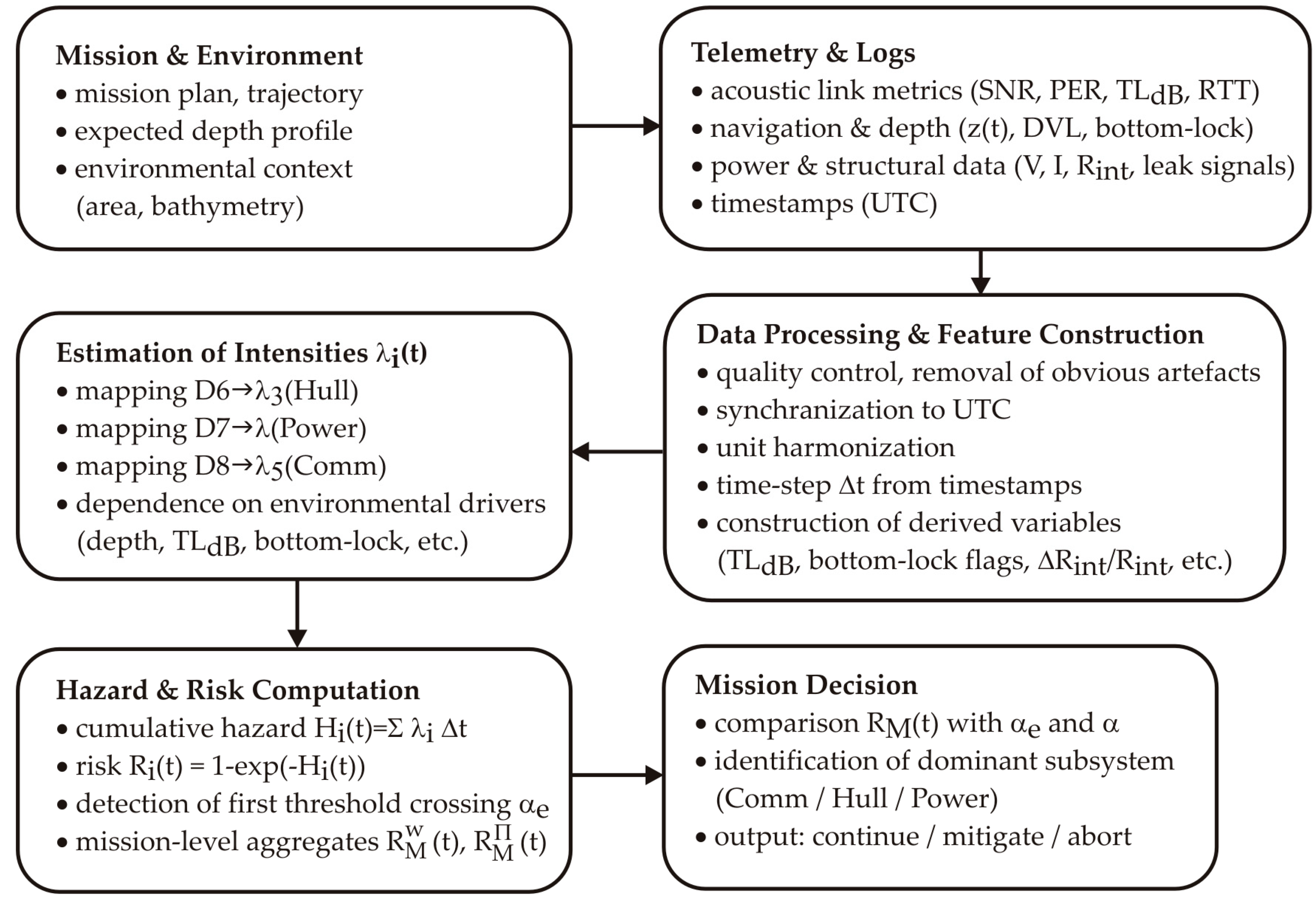Thirdly, we extend subsystem-level results into a mission-level decision with clear interpretation (time of first warning, margin to abort threshold, persistence relative to S2/S3/S4), while maintaining notational consistency with Section 3 and continuity with subsequent sections (data, results, discussion). The complete structure of this flow is outlined in the scenario diagram shown in Figure 1.

In a broader research context, the proposed approach addresses the gap between theoretical modeling and operational practice by linking the NH-CTMC formalism [1,2] with high-resolution telemetry, UTC synchronization, and explicitly defined operational thresholds. The scarcity of empirical works after 2015, particularly those reporting λ_i(t), H_i(t), R_i(t), and the “continue/abort” decision within a single, coherent framework, highlights the need for further studies and reporting standardization. The results presented in the following sections aim to provide such a reference, both as a baseline for mission comparisons and as a starting point for sensitivity analysis, subsystem extensions, and coupling with risk planning policies [13,14,15,16,17].

2. Characteristics of AUV Subsystems

The MBG-AUV platform has a modular architecture. Functionally, it comprises seven interacting subsystems: power (Power), propulsion (Propulsion), control and navigation (Control/Nav), communications (Comm), payload sensors (Sensors), hull/structural integrity (Hull/Structure), and software with mission management (Software/Mission Management). These subsystems operate in close interaction with the marine environment, including depth/pressure, the sound speed profile and propagation losses (TL_dB), currents, temperature, and salinity. A summary of subsystem roles, interaction vectors, and utilized signals is provided in

Table 1. Operating/environmental factors and affected subsystems (MBG-AUV).

Factor (Symbol)	Mechanism of Action	Most Exposed Subsystems	Typical Effect in Operation	Example Signals/Metrics
Depth/pressure (z, p)	Higher stresses, leak risk	Hull/Structure, Power (compartments), Pressure sensors, Control/Nav	↑λ(hull); ψ0→4 (breach); harder safe surfacing	p(z), leak flag, strain/AE, depth-sensor drift
Water temperature (T)	Conductivity/viscosity change, aging	Power and electronics, Propulsion	↑λ(power/elec); ψ0→3 (thermal throttling → steering margin)	V–I under load, Rint trend, TESC, Tcell, CPU temp
Salinity/conductivity (S, σ)	Corrosion, insulation degradation	Hull, Power, Comm (connectors), Sensors	↑λ(hull/power); ψ0→3 (shorts)	Leakage current, connector logs, BMS faults
Currents/waves (u)	Higher hydrodynamic load, asymmetry	Propulsion, Control/Nav, Power	↑λ(prop); ψ0→3 (loss of controllability); μ1 harder	Ithr vs. RPM, differential loads, energy/km
Turbidity/optical attenuation (κ)	Optical SNR drop	Sensors (vision)	↑λ(sensors) → quality loss; ψ0→2 (switch to backup)	Camera SNR, HDR/ISO, contrast/scatter, detection errors
Acoustic propagation loss/noise (TLdB, Na)	Link/DVL/sonar SNR drop	Comm, Control/Nav (DVL), Acoustic sensors	↑λ(comm/nav); ψ0→3 (link loss), μ may fail remotely	SNR, PER/BER, RTT, packet loss, DVL bottom-lock quality
Biofouling/growth	Drag increase, sensor attenuation	Propulsion, Sensors, Hull	↑λ(prop/sens) (degradation); ψ0→2	More power at same speed, sensor SNR drop
Collision/entanglement/impact	Instant mechanical damage	Hull, Propulsion, Sensors, Control/Nav	ψ0→4 (or ψ0→3)	Shock accel., thruster stall, attitude alarms
Local leak (L)	Water ingress, shorts, buoyancy loss	Hull, Power, Electronics	ψ0→4 (breach); ↑λ(corrosion); μ less effective	Humidity/conductivity probes, flood sensors, voltage sag
Magnetic/EM disturbances	Compass error, electronics interference	Control/Nav, Comm	↑λ(nav); ψ0→3 (course error → loss of position)	Heading deviation, IMU/DVL inconsistency
Link geometry/distance (R, multipath)	Higher TL, worse connectivity	Comm	↑λ(comm); ψ0→3 (blackout)	SNR vs. range, windowed PER, missing ACK
Mission time/fatigue	Accumulated wear and drifts	Power, Propulsion, Sensors, Hull	↑λ(all) after thresholds	Rint drift, higher energy/km, sensor bias
Electronics temperature (Telec)	Derating, throttling, resets	Power/ESC, Software, Comm	↑λ(elec/sw); ψ0→3 (watchdog)	TESC/CPU, watchdog/reset counters
Proximity to seafloor/terrain	Contact risk, DVL issues	Control/Nav, Hull, Sensors	↑λ(control); ψ0→3 (bottom-lock loss, contact)	DVL quality, depth error, proximity alarms

(factors → subsystems), while the operational interpretation of state transitions and typical triggers in the data are presented in

Table 2. Interpretation of graph transitions (common across subsystems).

Transition	Type	Most Frequent Triggers (Conditions)	What is Observed (Signals)
S0 → S1 (λ)	degradation	Long-term T↑/z↑/S↑, biofouling onset	Slight ↑power per km, sporadic packet errors, small sensor drift
S1 → S2 (λ1)	degradation	Increasing hydro loads, battery aging	Rint↑, energy reserve drop, thruster asymmetry
S2 → S3 (λ2)	degradation	Energy limit at currents; loss of references	No DVL bottom-lock, growing depth/heading error
S3 → S4 (λ3)	degradation	Controller cannot stabilize; actuator saturation	High control error, regulator alarms, oscillations
S0 → S2 (λ4)	jump	Critical sensor failure with redundancy; watchdog	Step-like performance drop, mode change
S0 → S3 (λ5)	jump	Acoustic-link blackout; micro-leak with trend; sudden energy-margin fall	PER spikes, missing ACK, leak trace L > 0↑, Eres/Eneed↓
S3 → S0 (μ1)	restoration	Switch to reserve; recovered link; stabilized controller	“backup” flags, link regained, errors stabilize
S4 → S0 (μ)	restoration	Drop-weight + surfacing; hard reset; beacon recovery	Emergency telemetry returns; recovery mode active
S4 → L (ν)*	absorbing loss	Deep flooding; power lost beyond reserve; entanglement/collision	No telemetry after T*, no ACK from buoy/beacon

.

Explanation of notation:

• Arrows of the type S_i → S_j denote a directional transition in the five-state classification graph from the source state S_i to the target state S_j. The intensities λ and μ describe degradation and regeneration processes, respectively. Transitions marked as “jump” represent sudden, discontinuous state changes that skip intermediate levels.
• The symbol * (asterisk) next to S₄ → L (ν)* indicates that state L is absorbing, and once it is reached, the object cannot return to any operational state.
• The designation T* refers to the cut-off time, after which the lack of a telemetric response or lack of confirmation from the buoy/beacon is treated as a clear signal of entering the absorbing state L (loss of the object).
• The symbol ↑ indicates an increase in the value of a given parameter or intensity (e.g., ↑λ—increased degradation intensity, ↑power—higher power demand). Similarly, the symbol ↓ (if present) indicates a decrease in the value of a parameter.

For clarity, we note that transitions listed in Table 2 are typically accompanied by measurable changes in the corresponding signals (e.g., a noticeable increase in PER during communication windows for S0→S1). These examples are representative only and are not intended to redefine the structure of the table.

At the power level, the BMS monitors cell voltage, current, and temperature, as well as health indicators (internal resistance), enabling the assessment of energy reserves and the detection of power-limiting episodes. The propulsion subsystem, equipped with ESC controllers, generates thrust, ESC currents, and RPM, and the temperatures reveal load asymmetries and thermal phenomena. The control and navigation layer stabilizes the trajectory using the IMU, depth sensor, and DVL; the performance quality is reflected in depth/course deviations, the depth profile z(t), and bottom-lock availability. Communications are provided by an acoustic modem (with optional RF after surfacing), the channel quality is characterized by SNR, PER/BER, RTT, and TL_dB exposure, with exchanges occurring in transmission windows. Payload sensors (optical, acoustic, and others) provide mission-relevant data, for whose quality/detection indicators are monitored. Structural integrity is tracked by flooding and stress sensors, with the depth profile and leak-signal dynamics being critical. Software supervision manages the mission plan, safety, and emergency modes (watchdog, resets, recovery procedures).

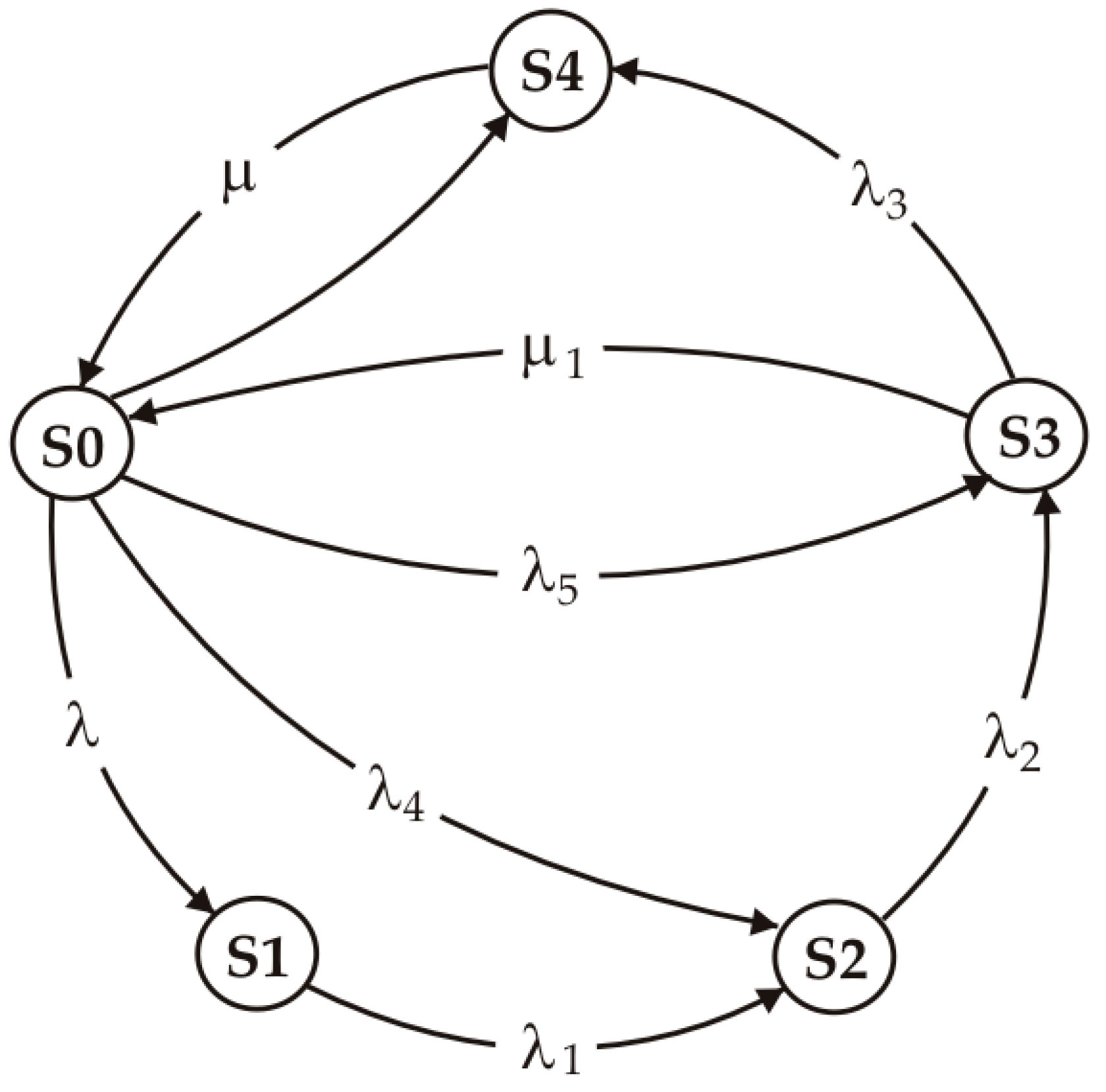
The operational logic of the subsystems is described by the state graph (Figure 2) S0–S4 (the “without L” variant described in Section 3). S0 denotes nominal operation, S1 indicates symptoms (warning), S2 corresponds to reduced performance, S3 to limited capability (fallback/emergency mode), and S4 to the critical state. We admit progressive degradations along the chain S0→S1→S2→S3→S4 (labeled λ, λ₁, λ₂, λ₃) jumps bypassing levels (λ₄ for S0→S2, λ₅ for S0→S3), as well as recoveries to the safe mode μ₁ (S3→S0—function restoration or switchover to redundancy) and μ (S4→S0—emergency procedures). Degradations correspond to the gradual deterioration of conditions or subsystem health (rising TL_dB, loss of control reference, decreasing energy margin), jumps reflect abrupt events (redundancy-triggered reset, communication blackout), and μ arcs represent real opportunities to restore function and continue the mission after effective intervention. Typical triggers include PER/BER spikes and missing ACK (S0→S3 in communications), bottom-lock loss and increasing depth/course error (S2/S3 in control), or the appearance of a leak signal (escalation S3→S4 in the hull).

For a complete picture of the interdependencies among the seven subsystems, a hub-and-spoke view is useful. The circular variant, shown in Figure 3, treats Software/Mission Management as the coordinating node. Blue arrows from this node to the others denote the primary control and telemetry relationship (data/cmd). The relation between Control/Nav and Propulsion, labeled actuation (orange arrow), corresponds to actuator signals within the control loop. Red arrows from Power to all subsystems indicate power supply (DC bus). The dashed green arrow from Hull/Structure to Software, Control, and Power represents safety couplings and constraints (flooding detection, overpressure/depth exceedance). The Environment remains an external factor (water column and seabed) that affects Communications, Control/Nav, and Hull/Structure, but it does not constitute an eighth subsystem and, therefore, is not represented as a separate block.

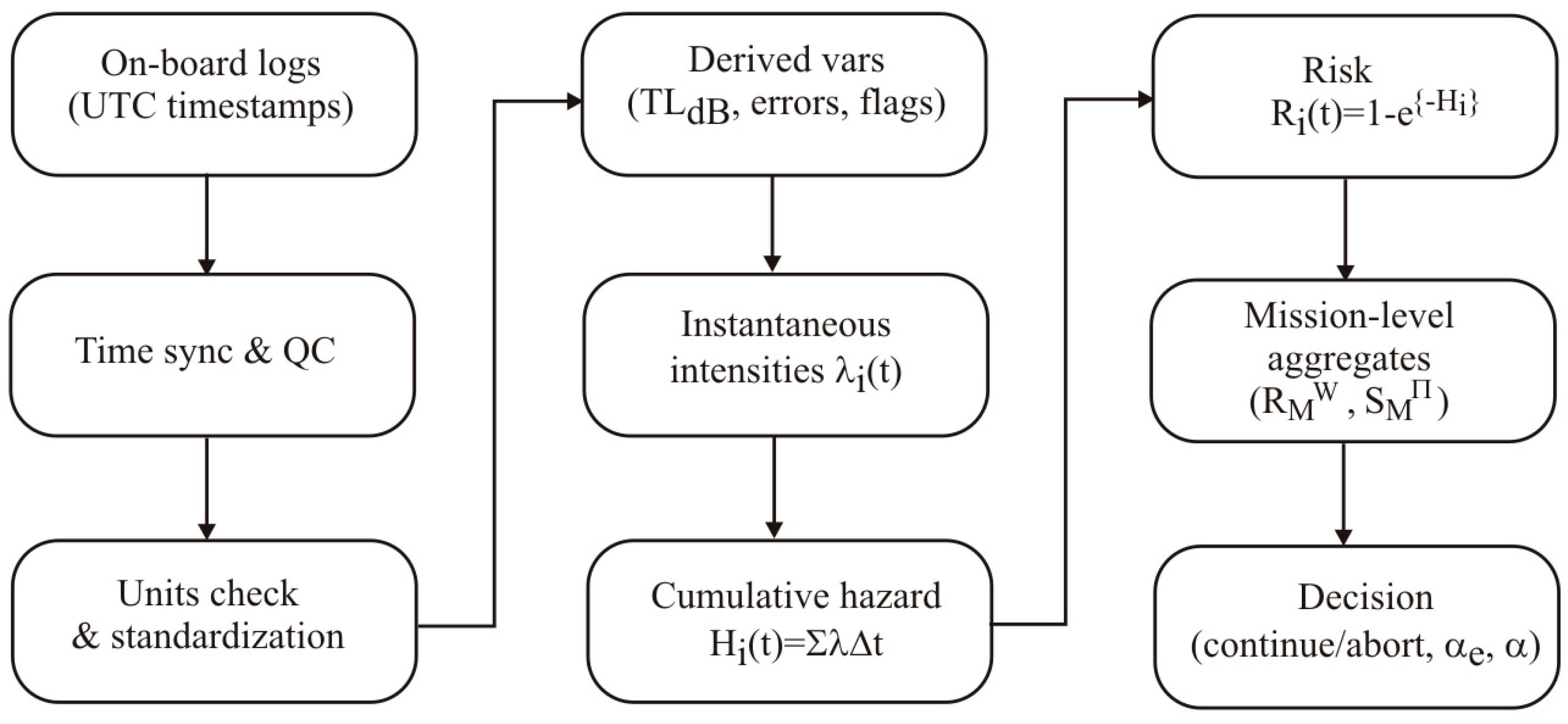
To provide context, a simple data flow is also presented, linking the subsystems with the subsequent analysis, onboard logs (UTC) → synchronization and quality control → unit standardization → construction of derived variables (TL_dB, control errors, quality flags) → estimation of instantaneous transition intensities λ_i(t) → accumulation of exposure (hazard) and risk → mission-level aggregates and the “continue/abort” decision. Figure 4 ensures terminological consistency with Table 1 and Table 2, and sets the stage for computations in the later sections without delving into calculation details here.

The structured characterization presented in Section 2 provides a shared technical vocabulary and a consistent interpretive framework for subsequent analysis. The same states and relationships shown in the figures are later supplied with observations, transformed into intensities (in s⁻¹), accumulated over the mission timeline, and applied in the “continue/abort” assessment with an explicit reference to the specific subsystem, profile segment, and transition arrow in the graph.

3. Mathematical Model

At this stage, we move from qualitative description to formal representation. The structure of the process follows the previously shown transition graph (Figure 2), where degradation steps dominate, operational jumps occur occasionally, and recovery switches appear only in states of advanced degradation. Transition intensities are conditioned on the mission profile w(t) = {z(t), T(t), S(t), u(t), κ(t)}, ensuring that the model is anchored in actual data.

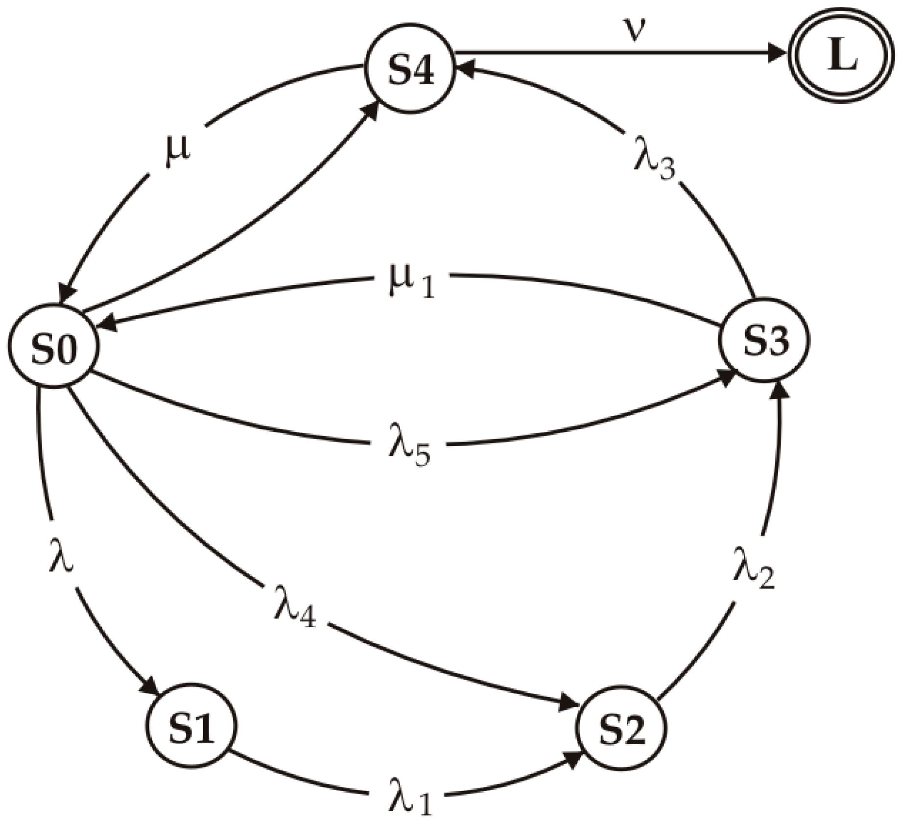
For mission risk analysis, we extend the graph (Figure 5) with an absorbing state L (loss of the platform), which is reachable exclusively from the failure state through intensity ν: S4→L. Formally, each primary subsystem (power, propulsion, control/navigation, communications, sensors, hull, software) is described by a continuous-time process with five condition levels S0–S4. Admissible transitions include stepwise degradations S0→S1→S2→S3→S4, operational jumps S0→S2 and S0→S3, and recoveries to the operable state S3→S0 and S4→S0.

We treat the transition intensities as functions of the mission profile wherever justified by the structure of inter-subsystem influences. In this way, both the risk of escalation and the likelihood of recovery follow directly from the operating conditions. This structure is expressed in matrix form as the generator Q, which serves as the starting point for further derivations of risk measures and decision rules.

$$Q^i=\left[\begin{array}{cccccc}-(\lambda +{\lambda }_4+{\lambda }_5)& \lambda & {\lambda }_4& {\lambda }_5& 0& 0\\ 0& -{\lambda }_1& {\lambda }_1& 0& 0& 0\\ 0& 0& -{\lambda }_2& {\lambda }_1& 0& 0\\ {\mu }_1& 0& 0& -\left({\lambda }_3+{\mu }_1\right)& {\lambda }_3& 0\\ \mu & 0& 0& 0& -(\mu +v)& v\\ 0& 0& 0& 0& 0& 0\end{array}\right]$$

(1)

Expanded Kolmogorov equations derived from the generator Q(t):

$$P_0\left(t\right)=-(\lambda +{\lambda }_4+{\lambda }_5)P_0+{\mu }_1{P}_3+\mu P_4$$

(2)

$$P_1\left(t\right)=\lambda P_0-{\lambda }_1{P}_1$$

(3)

$$P_2\left(t\right)={\lambda }_1{P}_1-{\lambda }_2{P}_2+{\lambda }_4{P}_0$$

(4)

$$P_3\left(t\right)={\lambda }_2{P}_2-({\lambda }_3+{\mu }_1)P_3+{\lambda }_5{P}_0$$

(5)

$$P_4\left(t\right)={\lambda }_3{P}_3-(\mu +\nu )P_4$$

(6)

$$P_L\left(t\right)=\nu P_4$$

(7)

Normalization and consistency condition. For a time step Δt (in the data: 5 min), on the interval [t_k,t_{k+1}), we take Q_k = Q(t_k) and compute: p_{k+1} = p_k · exp(Q_k · Δt), where p_k = [P₀,P₁,P₂,P₃,P₄,P_L] at time t_k.

$${\displaystyle \frac{d}{dt}}\left(\sum _{k=0}^4{P}_k(t)\right)=-\nu P_4(t)=P_L(t) ⟹ \sum _{k=0}^4{P}_k\left(t\right)+P_L(t)\equiv 1$$

(8)

In this expression, the numerator corresponds to the sum of transition intensities λ_i(t) in Q(t) that lead from S3 to more degraded states, while the denominator contains all outgoing intensities from S3 (both degradative and restorative). This highlights that the probability reflects the balance between escalation pathways and available recovery routes.

For practical purposes, two classes of quantities are useful. The first describes the race between escalation and recovery in S3, namely the probability that from S3, the system escalates to S4 before recovery occurs:

$$P(S3⟶S4 before L)={\int }_0^{\infty }\mu (t)exp\left(-{\int }_0^t\left[\mu \left(s\right)+{\mu }_1\left(s\right)\right]ds\right)dt$$

(9)

Here, the restorative terms μ_i in Q(t) represent transitions returning the system from S3 to safer states (typically S1 or S0), and compete directly with the degradative rates. The ratio, therefore, quantifies the likelihood that recovery occurs before any further degradation.

$$P(S4⟶S0 instead of S3⟶S0)={\int }_0^{\infty }{\lambda }_3(t)exp\left(-{\int }_0^t\left[{\lambda }_3\left(s\right)+\nu \left(s\right)\right]ds\right)dt$$

(10)

In the case of S4, the transition ν to the absorbing loss state L represents the only degradative pathway, while μ_L denotes the available restorative transition. The resulting probability thus expresses the chance that the platform is recovered, rather than lost, once S4 is reached.

Including state L does not alter the logic of reserve management, as it remains a state reachable only after entering S4. The parameter ν encapsulates scenarios in which the recovery S4→S0 does not occur during the mission; it corresponds, for example, to severe flooding, permanent immobilization, or destruction of critical components.

The elements of the matrix have a physical interpretation and are not chosen arbitrarily; each transition intensity is a function of environmental conditions and, where structurally justified, the states of other subsystems. In this way, both the risk of escalation and the chance of recovery follow directly from the mission profile and the reserve architecture. From this perspective, two quantities of key practical importance are obtained immediately—the probability that in state S3, escalation to S4 occurs before recovery, and the probability of recovery from S4 instead of unit loss. The former reflects the balance between degradation dynamics and the effectiveness of switchover to redundancy, while the latter captures the compromise between recovery procedures and the risk of absorption.

The subsequent description relies on observed signals and their conditional emissions, which makes it possible to determine the posterior distributions of individual subsystem states, to aggregate them into the overall system state in accordance with continuation tolerances, and to apply a unified mission abort rule, followed by the reporting of risk measures and cumulative hazards at mission completion.

Transition intensities are treated as functions of the mission profile w(t), including in particular depth, z(t), temperature T(t), salinity S(t), current velocity u(t), and turbidity κ(t). Where justified by vehicle design, inter-subsystem couplings are admitted (reduced power health increases the degradation rate of propulsion). The unified representation takes the form:

$${\theta }^{ \left(i\right)}\left(t\right)={\theta }_0^{ \left(i\right)}\left\{{\beta }^{ \left(i\right) T}w \left(t\right)\right\}·{ g}^i\left(X_{-i}\left(t\right)\right)$$

(11)

where θ—denotes any of the transition intensities {λ,λ₁,λ₂,λ₃,λ₄,λ₅,μ₁,μ,ν}, and g⁽ⁱ⁾ is a function capturing the influence of the states of other subsystems (g = 1 + ρ1{$X_{power }\ge 2$). Importantly, two measures with clear interpretation follow directly from this construction—the probability that in state S3, escalation to S4 occurs before recovery, equal to ${\displaystyle \frac{{\lambda }_3}{{\lambda }_3+{\mu }_1}}$, the probability of recovery from S4 (instead of loss), equal to t ${\displaystyle \frac{\mu }{\mu + \nu }}$. These design levers clearly show what is worthwhile reinforcing, and why.

The states themselves are hidden; we do not observe them directly, but only through measurement streams characteristic of each subsystem. For power, these include V(t), I(t), internal cell resistance, and temperature; for propulsion, thruster currents and RPM along with controller temperatures; for control and navigation, depth and course error, DVL bottom-lock quality, and IMU pressure consistency; for communications, SNR, PER/BER, and delays; for sensing, SNR measures of optical or acoustic channels; for the hull, leak signals and possibly structural acoustics; and for software, loop times and watchdog events. We assume that the emission distribution of these observations depends on the current state and conditions, for example:

$$y_i\left(t\right)/X_i\left(t\right)=k~N\left({\mu }_{ik}\right(w\left(t\right)),{\sum }_{ik}(w\left(t\right)\left)\right)$$

(12)

However, nothing prevents the use of nonlinear models or mixtures in specific channels. On this basis, we determine the posterior distributions π_ik(t) = P{X_i(t) = k/Y_0:t,w_0:t}, The state of the entire vehicle must synthesize divergent information from multiple subsystems. Aggregation cannot be purely arithmetic; it must reflect operational significance. We therefore introduce continuation tolerances τ_i and criticality levels. The principle is simple and consistent with practice: mission-blocking subsystems (power, propulsion, control/navigation) cannot reach S2 without affecting the global state; in other subsystems, certain deviations are permissible (hull in S1, software in S2) without changing the overall state. In algebraic form, we define penalties p_i = α_i [X_i-τ_i]₊ with coefficients α_i reflecting subsystem criticality, compute E(t) = max_ip_i(t), and map E onto levels S0…S4 through three decision thresholds. In practice, instead of raw states X_i, we use their posteriors π_ik(t), which yields a smooth, probabilistic assessment of the system state.

The mission abort decision is a stopping problem, but in operational terms, it can be stated clearly—abort if the probability that the aggregated state has reached an unacceptable level (at least S2) exceeds a prescribed threshold, or if the communication quality remains below the required minimum for a specified duration, rendering risk supervision unreliable. In compact notation:

$$\tau =inf\left\{t: P\left(G\left(X\left(t\right)\right)\ge S2/Y_{0:t}\right)\ge \alpha \right\} or {\displaystyle \frac{\widehat{PER}(t)\ge { \alpha }_{link}}{\Delta t}}$$

(13)

We see that both thresholds (α for the state and α_link for the communication link) have an unambiguous operational interpretation and can be calibrated to the mission profile.

Risk measures and post-mission assessment follow directly from the transition matrix. If, from Q, we extract the submatrix of transitions among transient states (the first 5 × 5, excluding L) and denote it by T, and if we write the transitions to L as a vector t (nonzero only in the row corresponding to S4), then the distribution of the time to AUV loss is given by

$$P({\tau }_L\le T)=1-e_{S0}^T\mathrm{e}\mathrm{x}\mathrm{p}(T · T)1, E\left[{\tau }_L\right]=-e_{S0}^T{T}^{-1}1$$

(14)

Analogous constructions are applied to compute the probability of entering {S3, S4} by time T for any subsystem. After mission completion, we report not only these probabilities and the final posteriors π_ik(T) but also the cumulative degradation hazard:

$${CumHaz}_i(T)={\int }_0^T\sum _{k=0}^2{\lambda }_k^{\left(i\right)}\left(t\right){\pi }_{ik}\left(t\right)dt$$

(15)

It is a natural numerical measure of the “consumed reliability budget” under given conditions.

To preserve concreteness and comparability across subsystems, The

Table 3. Subsystems, observations, factors, example intensities.

Subsystem	Key Observations yi	Environmental/Operational Factors w	Example Intensities
Power system	V, I, Rint, Tcell	T, z	λ, λ1 = λ0 exp(β1T + β2z); λ4 = κ1 1{ΔR/R > θR}; μ = μ0 exp(−ηTT)
Propulsion	Ithr, RPM, TESC	u, T	λ2 = λ2,0 exp(γu); (λ5= κ2)
Control and navigation	depth/heading error, DVL lock, IMU-pressure	u, z	λ2 = λ2,0 exp(η1u); λ5 = κ3 1{DVL lost}; μ1 = μ1,0 exp(−ηzz)
Comm	SNR, PER/BER, RTT	transmission loss (TL), noise Na	λ = λ0 exp(ξ TL); λ5 = κ4 1{PER > θPER ∧ Δt}
Mission sensors	optical/acoustic SNR, biases	κ, z	λ1 = λ1,0 exp(ζκ); λ4 = κ5 1{redundant sensor failure}
Hull/structure	leak sensors L, AE/strain	z, S	λ3 = λ3,0 exp(α1z + α2S); λ5 = κ6 1{L > Lwarn}; ν = ν0 1{L > Lcrit}
Onboard software	watchdogs, loop time, TCPU	TCPU	λ = λ0 exp(χTCPU); λ4 = κ7 1{watchdog reset}

below compiles the typical diagnostic observations, environmental factors, and representative forms of transition intensities in one place. All formulas are consistent with the general form θ₀exp{β^⊤w} and with the logic of jumps and recovery.

Since the model is meant to serve decision-making rather than elegance for its own sake, we conclude it with a procedure for estimating quantities not directly available from mission logs and environmental data. The “continuous” intensities (λ,λ₁,λ₂,λ₃) are calibrated as functions of covariates w(t) (in the style of Eyring/Cox), the jump intensities (λ₄,λ₅) are identified through event models based on defined triggers (loss of DVL, reset, thruster asymmetry, micro-leak), and the recovery and loss intensities (μ₁,μ,ν) are estimated from observed recovery episodes and actual loss cases. We fit the emission parameters μ_ik(w), Σ_ik(w) in parallel, so that filtering over the above process yields reliable posteriors ${\pi }_i^k$(t). Finally, for each subsystem, we compute the probability of entering {S3,S4} by time T, the distribution of the time to the first such entry, the cumulative hazard CumHazi(T) and the terminal state distribution ${\pi }_i^k$(T). For higher states, we obtain neat closed-form expressions ${\displaystyle \frac{{\lambda }_3}{{\lambda }_3+{\mu }_1}}$ i ${\displaystyle \frac{\mu }{(\mu + \nu )}}$, which synthesize the risk of escalation and the chance of recovery. For the entire AUV, we report the probability of a “stop” decision according to the stopping rule, and the probability of loss before the end of the mission T; both quantities follow directly from the transition matrix and require no arbitrary presets.

Thus, the consistently derived model integrates three levels of description, physics, statistics, and decision, into a single coherent narrative, starting from degradation phenomena and reserve architecture, formalizing dynamics on the transition graph, embedding actual measurements, and concluding with unambiguous evaluation rules and action choices. In this way, the chapter provides a complete foundation for the subsequent parts, data acquisition, calibration, and finally, the presentation of results for reference missions.

4. Data Sources and Processing

At this stage, we move from the conceptual description of states to the data that support the operational decision, whether to continue the mission or abort it. The perspective is purely operational: we monitor how the system trajectory approaches states S3 and S4, and whether effective recovery actions occur S3→S0 (μ₁) as a switchover to redundancy, and S4→S0 (μ) as a forced recovery (surfacing). These events, together with their environmental context, form the measurable background for the “continue/abort” decision.

The following are presented data provenance (

Table 4. Data sources and preprocessing (provenance and usage).

Source/System	Data Provenance	Signals (Symbols)	Frequency/Timestamp	Units	QC (Checks)	Derived Variables (Examples)	Model Usage (λ/ψ/μ)
Power	Onboard BMS logs (MBG AUV archive, mission [ID], firmware [ver])	V, I, Rint, Tcell, Eres/Eneed	1–10 Hz/UTC	V, A, Ω, °C, —	outliers, saturations, missing records	ΔRint/Rint, discharge/SoC trends, throttling episodes	λP = λP(S0→S1); ψ0→1 thresholds; info for μ (energy-recovery)
Propulsion	ESC/thruster logs (MBG AUV archive, mission [ID], firmware [ver])	Ithr(A/B), RPM(A/B), control demand, TESC	1–50 Hz/UTC	A, RPM, —, °C	asymmetry spikes, sensor dropouts, actuator saturation	current asymmetry, torque proxy, load u	λprop; ψ0→2 (asymmetry > θasym), ψ2→3 (saturation > θsat); μ (mode change)
Control/navigation	IMU, DVL, depth, flight-controller logs	heading/depth errors, z(t), IMU drift, DVL bottom-lock	10–100 Hz/UTC	°, m, —	vector consistency, drift, DVL lock	bottom-lock flags, drift rate, instability windows	λctrl (affects S2/S3); ψ0→2/ψ2→3; contributes to S2→S3, S3→S4
Comm	Acoustic/RF modem telemetry (SNR, PER/BER, RTT), comm windows	SNR, PER/BER, RTT, TLdB	event-driven/packet-time (UTC)	dB, —, ms, dB	sequence consistency, timeouts, missing ACK	windowed PER, mean TLdB	λC (e.g., λC ∝ exp(ξ·TLdB)); ψ0→3 (blackout), ψ0→2 (high RTT)
Sensors (opt./acoustic)	Sensor streams and quality flags	SNR, quality/detection flags	1–30 Hz/UTC	dB, —	spikes, buffer drops, saturation	quality metrics (HDR/ISO, scatter), detection error	ψ0→2 (functional transitions); covariates to λsens
Hull/structure	Pressure/depth, flooding/leak sensors	z(t), structural stress S, leak L	1–10 Hz/UTC	m, —, —	physical ranges, no unrealistic jumps	depth trend, leak onset/growth	λH (e.g., λH ∝ exp(α1z + α2S)); ψ0→3 (L > 0), ψ3→4 (L↑)
Environment	CTD/ADCP, models/buoys	T(t), S(t), u(t), κ(t), TLdB, Na	0.1–1 Hz/UTC or by segments	°C, PSU, m/s, —, dB, —	physical ranges, continuity	TLdB, hydrodynamic load indices	covariates in λ (e.g., λ ∝ exp(β1T + β2z))

Units (symbols) glossary. V—volt (electric potential), A—ampere (current), Ω—ohm (internal resistance R_int), °C—degree Celsius (temperature), RPM—revolutions per minute, ms—millisecond, s—second (hazards in s⁻¹), Hz—samples per second, dB—decibel (SNR, TL_dB), m—meter (depth z), m/s—meter per second (currents u), PSU—Practical Salinity Unit, “—”—dimensionless indicator (flags, ratios, PER/BER), SNR—signal-to-noise ratio (dB), PER/BER—packet/bit error rate (fraction), RTT—round-trip time (ms), TL_dB—transmission loss in dB, κ—optical turbidity/attenuation index (dimensionless), N_a—acoustic noise/path index (dimensionless).

), mission profile D1–D14 with instantaneous intensities λ and cumulative hazard CumHaz (

Table 5. Mission profile and hazards (D1–D14).

D1	D2	D3	D4	D5	D6	D7	D8	D9	D10	D11	D12	D13	D14
03.04.2025 12:23	50.0	18.00	34.800	71.0	0.000001	0.000002	0.000071	0.000363	0.000598	0.021243	0.000363	0.000598	0.021019
03.04.2025 12:28	79.2	17.08	34.833	71.6	0.000001	0.000002	0.000073	0.000771	0.001170	0.043243	0.000771	0.001170	0.042321
03.04.2025 12:33	108.3	16.17	34.867	72.2	0.000002	0.000002	0.000076	0.001231	0.001718	0.066026	0.001230	0.001716	0.063893
03.04.2025 12:38	137.5	15.25	34.900	72.8	0.000002	0.000002	0.000079	0.001748	0.002242	0.089621	0.001747	0.002239	0.085722
03.04.2025 12:43	166.7	14.33	34.933	73.3	0.000002	0.000002	0.000081	0.002331	0.002743	0.114056	0.002328	0.002739	0.107792
03.04.2025 12:48	195.8	13.42	34.967	73.9	0.000002	0.000002	0.000084	0.002986	0.003223	0.139362	0.002982	0.003217	0.130087
03.04.2025 12:53	225.0	12.50	35.000	74.5	0.000002	0.000002	0.000087	0.003724	0.003682	0.165569	0.003717	0.003675	0.152588
03.04.2025 12:58	254.2	11.58	35.033	75.1	0.000003	0.000001	0.000090	0.004555	0.004121	0.192709	0.004544	0.004112	0.175278
03.04.2025 13:03	283.3	10.67	35.067	75.7	0.000003	0.000001	0.000094	0.005489	0.004541	0.220816	0.005474	0.004530	0.198136
03.04.2025 13:08	312.5	9.75	35.100	76.2	0.000004	0.000001	0.000097	0.006542	0.004943	0.249925	0.006520	0.004930	0.221141
03.04.2025 13:13	341.7	8.83	35.133	76.8	0.000004	0.000001	0.000100	0.007726	0.005327	0.280070	0.007697	0.005313	0.244269
03.04.2025 13:18	370.8	7.92	35.167	77.4	0.000004	0.000001	0.000104	0.009060	0.005695	0.311289	0.009019	0.005679	0.267498
03.04.2025 13:23	400.0	7.00	35.200	78.0	0.000005	0.000001	0.000108	0.010561	0.006047	0.343620	0.010505	0.006029	0.290802

D1—time_utc—UTC time (5 min intervals). D2—depth_m—depth z(t) in meters. D3—temp_C—water temperature T(t) in °C. D4—salinity_psu—salinity S(t) in PSU. D5—TL_dB—simple indicator of propagation losses (proxy for the communication link). D6–D8—lambda_hulls⁻¹ = λ₃(S3⟶S4), lambda_powers⁻¹ = λ(S0⟶S1), lambda_comms⁻¹ = λ₅(S0⟶S3)—instantaneous hazards (transition rates) for hull, power, and communications subsystems, in s⁻¹. D9–D11—CumHaz_hull, CumHaz_power, CumHaz_comm—cumulative hazard up to the given time (dimensionless), i.e., the sum—suma ∑λΔt. D12–D14—Risk_hull, Risk_power, Risk_comm—risk up to time t ≈ 1 − e^−CumHaz for the respective subsystem.

), as well as definitions of the indicators R(t) and the instant t_α used in decision-making and in subsystem-level summaries (

Table 6. Subsystem summary at T and first early-warning crossing (Risk ≥ 0.10).

Subsystem	CumHazi(T)	Riski(T)	Time When Risk ≥ 0.10 (UTC)	Minutes From Start	Dk (Segment at Cross)	Depth at Cross [m]	Data Coverage [%]
Hull	0.010561	0.010505	not reached	—	—	—	100
Power	0.006047	0.006029	not reached	—	—	—	100
Comm	0.343620	0.290802	3 April 2025 12:43 (UTC)	20	5	166.7	100

). Units of intensity: s⁻¹, Δt is derived from differences between consecutive timestamps.

Data originate from MBG-AUV onboard recorders (BMS/ESC logs and onboard buses), the navigation–control suite (IMU, DVL, depth), communication telemetry (acoustic modem and/or RF packets/ACK), operator event logs, and environmental profiling (CTD/ADCP, metoceanographic data). All streams are synchronized to UTC time.

Obtaining a measurement result begins with synchronizing all streams to UTC time. The data are then cleaned; and short gaps (<2Δt) are filled using controlled imputation. In practice, this refers only to very short single-sample gaps and is implemented as a linear interpolation between the two adjacent time-stamped measurements, ensuring that no artificial trends are introduced into the λ_i(t) calibration. Concurrently, units are standardized and ranges verified (sanity check). The entire procedure is fully replicable for any mission profile given access to the underlying telemetry streams, as all processing steps (UTC alignment, QC filtering, and exposure mapping) are deterministic and explicitly documented. From the prepared data, auxiliary variables are constructed (including TL_dB, R_int, thruster asymmetry, DVL bottom-lock signal, and event markers). At each time step, instantaneous hazard intensities are determined for the critical subsystems λ_hull, λ_power, λ_comm (D6-D8, in s⁻¹). Subsequently, hazard increments are accumulated H_i(t) = ∑λ_iΔt (D9-D11) and the indicators are computed R_i(t) = 1 − exp(−H_i(t)) (D12-D14). Finally, the quality of computations is verified (time coverage, monotonicity of H_i, non-negativity of λ_i) and decision summaries are prepared, namely R_i(T), t_α and mission-level aggregates.

Based on the synchronized streams, we construct a sequence of segments D1-D14, where each row describes a mission interval using environmental and load descriptors along with the corresponding model columns. We apply the following mapping of columns to model parameters: D6 = λ₃ (Hull, S3→S4), D7 = λ (Power, S0→S1), D8 = λ₅ (Comm, S0→S3), D9-D11 = CumHaz_i, D12-D14 = R_i.

From the time rows in Table 5 (5 min step), we extract (a) the final values at time T, and (b) the first exceedance of the early-warning level αₑ = 0.10 for each subsystem. For that moment, we report the UTC timestamp, the number of minutes since mission start, the row index Dk (counted from 1, in 5 min steps), and the depth at the time of exceedance.

Time format note: In the column Time, when Risk ≥ 0.10 (UTC), we report the UTC timestamp of the first exceedance of the 0.10 level. Preferred format: dd.mm.yyyy HH:MM (UTC). For full unambiguity, an ISO 8601 representation may be given in parallel 2025-04-03 12:43Z.

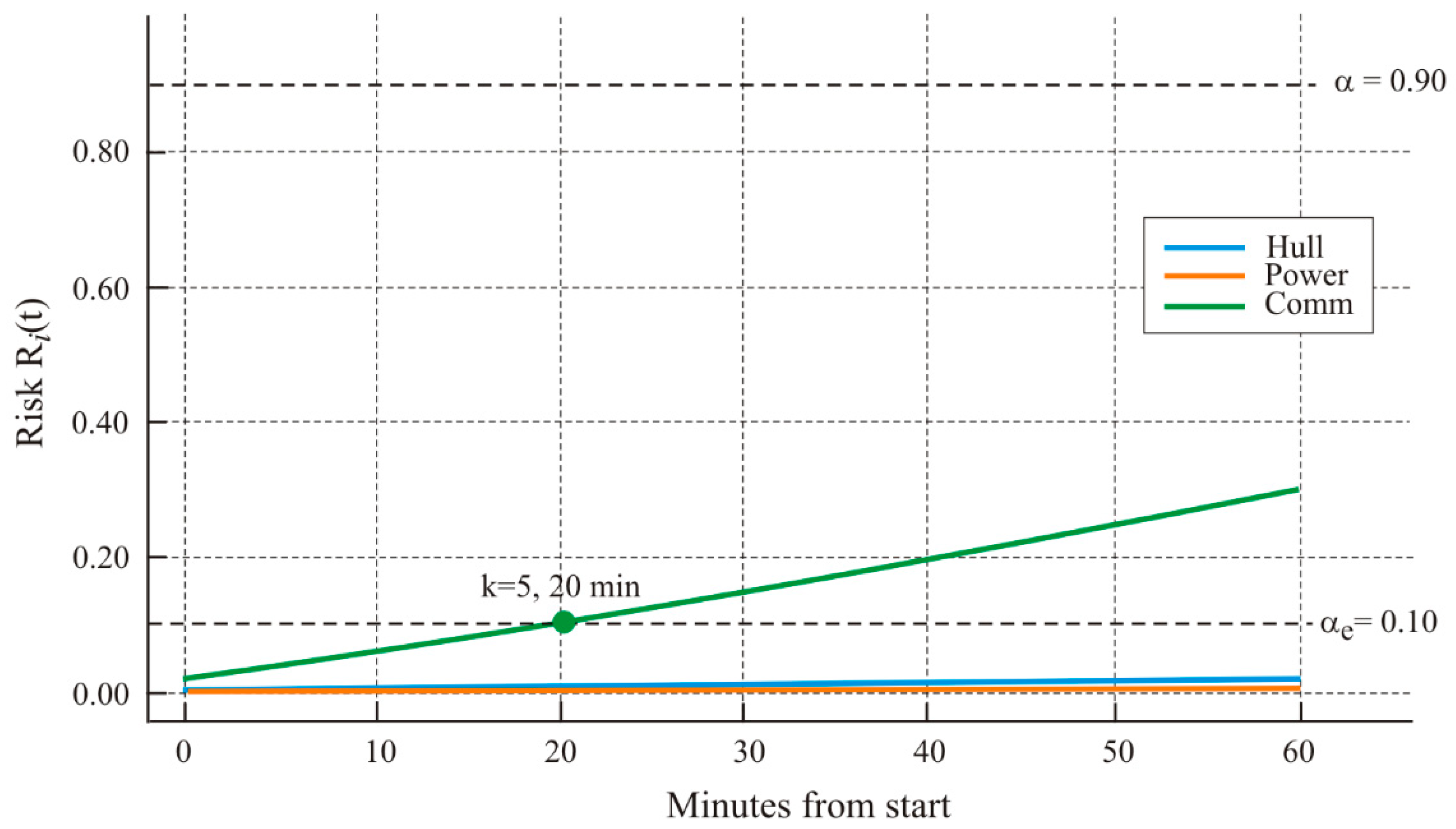
The Comm subsystem dominates both cumulative hazard and risk at time T and is the only one to exceed the warning threshold of 0.10; this occurs at k = 5 (~20 min after start, depth ~167 m). Hull and Power remain below 0.10 over the analyzed interval. In Section 5, we apply a higher decision threshold (α = 0.90); under such a stringent criterion, no subsystem reaches the threshold within this dataset.

Table 5 presents the mission timeline in five-minute steps, where each row corresponds to a successive underwater segment described by environmental conditions (depth, temperature, salinity) and communication difficulty (TL_dB). Alongside this, three current subsystem risks are shown (Hull/Power/Comm). These represent per-second values calculated for the given interval. Over time, the exposure accumulates, hence the monotonic growth of the CumHaz columns, while the Risk_i columns map this exposure onto the 0–1 scale, which is easier for operational interpretation. The final row of Table 5 gives the end-of-mission state, which directly feeds into Table 6, where subsystem-wise summaries and first exceedances of the warning threshold (here: 0.10; times reported in UTC) are collected.

Three operational measures were applied: (a) risk accumulation for each subsystem at time T (CumHaz_i(T) and Risk_i(T)), (b) the first warning signal—the first instant when the condition Risk_i ≥ α_e is met, reported with context (UTC time, minutes since start, row Dk, depth), and (c) the mission-level assessment. The values were derived directly from Table 5; the last row provided CumHaz_i(T) i Risk_i(T), and the first row with Risk_i ≥ αₑ was identified (with full context reported). The overall assessment is reported in two variants: a weighted average (with predefined weights www) and the “at least one event” variant (assuming independence). This set of indicators provides the basis for an unambiguous “continue/abort” qualification and highlights the segments requiring mitigation before the next deployment.

5. Results

The risk assessment is based on mission profile time-series data combined with the formal CTMC description and is intended to support the “continue/abort” decision. Three perspectives are of interest: the risk level at the end of the mission (T), any exceedances of the defined decision threshold, the overall picture through aggregated measures, and the contribution of individual segments. The table layout reflects this sequence values at T for each subsystem, followed by verification against the threshold α = 0.90, then, the mission-level assessment and identification of hot segments of the trajectory. Conventions remain consistent, intensities are given in s⁻¹, and Δt is computed directly from the data.

All configuration parameters listed in

Table 7. Mission summary (context).

Item	Value
Start time t0 (UTC)	[to be filled]
End time T (UTC)	[to be filled]
Number of segments (Dk)	13
Nominal Δt	5 min (from D1)
Duration (T − t0)	≈ 60 min
Early-warning threshold αe	0.10
Decision threshold α	0.90
Weights w (equal)	[1/3, 1/3, 1/3]
Weights wᴼ (operational)	[0.40, 0.35, 0.25]

follow directly from the native sampling resolution (Δt), the operational safety doctrine (αₑ and α), and the standard weighting policy used for mission-level evaluation. As summarized in Table 7, the mission consisted of 13 diagnostic segments with a nominal resolution of 5 min and a total duration of approximately 60 min. The corresponding end-of-mission risk measures for the main subsystems are presented in

Table 8. End-of-mission metrics (T).

Subsystem	CumHaz(T)	Risk(T)
Hull	0.010561	0.010505
Power	0.006047	0.006029
Comm	0.343620	0.290802

, which reports cumulative hazard and risk values at time T.

The values at T indicate that the Comm subsystem dominates the risk (≈0.291), while Hull and Power remain low (≈1.1% i ≈0.6%).

For clarity, the variable SegmentIndex used in

Table 9. Time to decision threshold α = 0.90.

Subsystem	Reached?	SegmentIndex	Depthm	Risk at Cross
Hull	no	-	-	-
Power	no	-	-	-
Comm	no	-	-	-

,

Table 10. Mission-level aggregates at T.

Aggregate	Value
${\mathit{R}}_{\mathit{M}}^{\mathit{w}}$(equal w = 1/3, 1/3, 1/3)	0.10244533
${\mathit{R}}_{\mathit{M}}^{\mathit{w}}$(oper w = [0.40, 0.35, 0.25])	0.07901265
${\mathit{R}}_{\mathit{M}}^{\mathbf{II}}$(independence)	0.30248296

,

Table 11. Top 3 segment contributions—Comm.

SegmentIndex	Depthm	ΔCumHaz	Share of Total [%]	Risk at Segment
12	400.0	0.001501	0.14212670	0.010505
11	370.8	0.001334	0.12631380	0.009019
10	341.7	0.001184	0.11211060	0.007697

,

Table 12. Top 3 segment contributions—Hull.

SegmentIndex	Depthm	ΔCumHaz	Share of Total [%]	Risk at Segment
0	50.0	0.000598	0.09889201	0.000598
1	79.2	0.000572	0.09459236	0.001170
2	108.3	0.000548	0.09062345	0.001716

and

Table 13. Top 3 segment contributions—Power.

SegmentIndex	Depthm	ΔCumHaz	Share of Total [%]	Risk at Segment
12	400.0	0.032331	0.09408940	0.290802
11	370.8	0.031219	0.09085327	0.267498
10	341.7	0.030145	0.08772772	0.244269

denotes the time-segment identifier (Dk) corresponding to the discrete 5 min intervals of the primary dataset described in Table 6. Each segment represents one temporal step within the data series D1–D14 (ranging from UTC timestamps, environmental parameters, and instantaneous transition rates to cumulative hazards and risk measures). Thus, SegmentIndex = Dk serves as a reference to the specific time step from which risk or degradation indicators such as Risk_hull, Risk_power, and Risk_comm were extracted. This indexing does not constitute an additional data column, but rather a positional pointer to the relevant row of the dataset used for model evaluation.

In the analyzed segment, no subsystem reaches the threshold α = 0.90—not even Communications, despite being the weakest subsystem.

In Table 9, the SegmentIndex column remains intentionally blank, as no mission segment fulfilled the threshold condition for the analyzed variable. In the subsequent Table 11, Table 12 and Table 13, the corresponding indices are explicitly provided to indicate the exact time segments at which the subsystem-specific risk values and degradation states were registered.

The weighted-average assessment is moderate (≈0.102, operational variant ≈ 0.079), while under the independence assumption the probability of at least one event by T is ≈0.302. For the operational decision $R_M^w$ was adopted with weights wᴼ = [0.40, 0.35, 0.25]. Since the threshold α = 0.90 was not reached, the decision is continued (no grounds for abort).

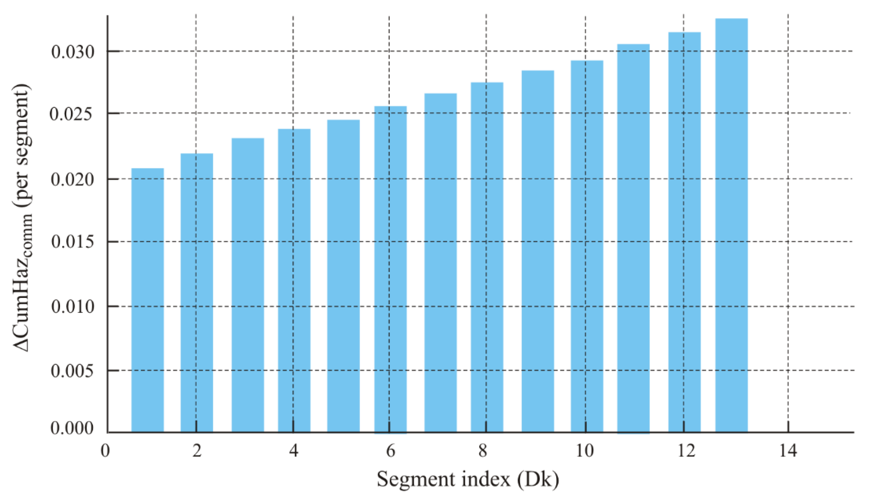
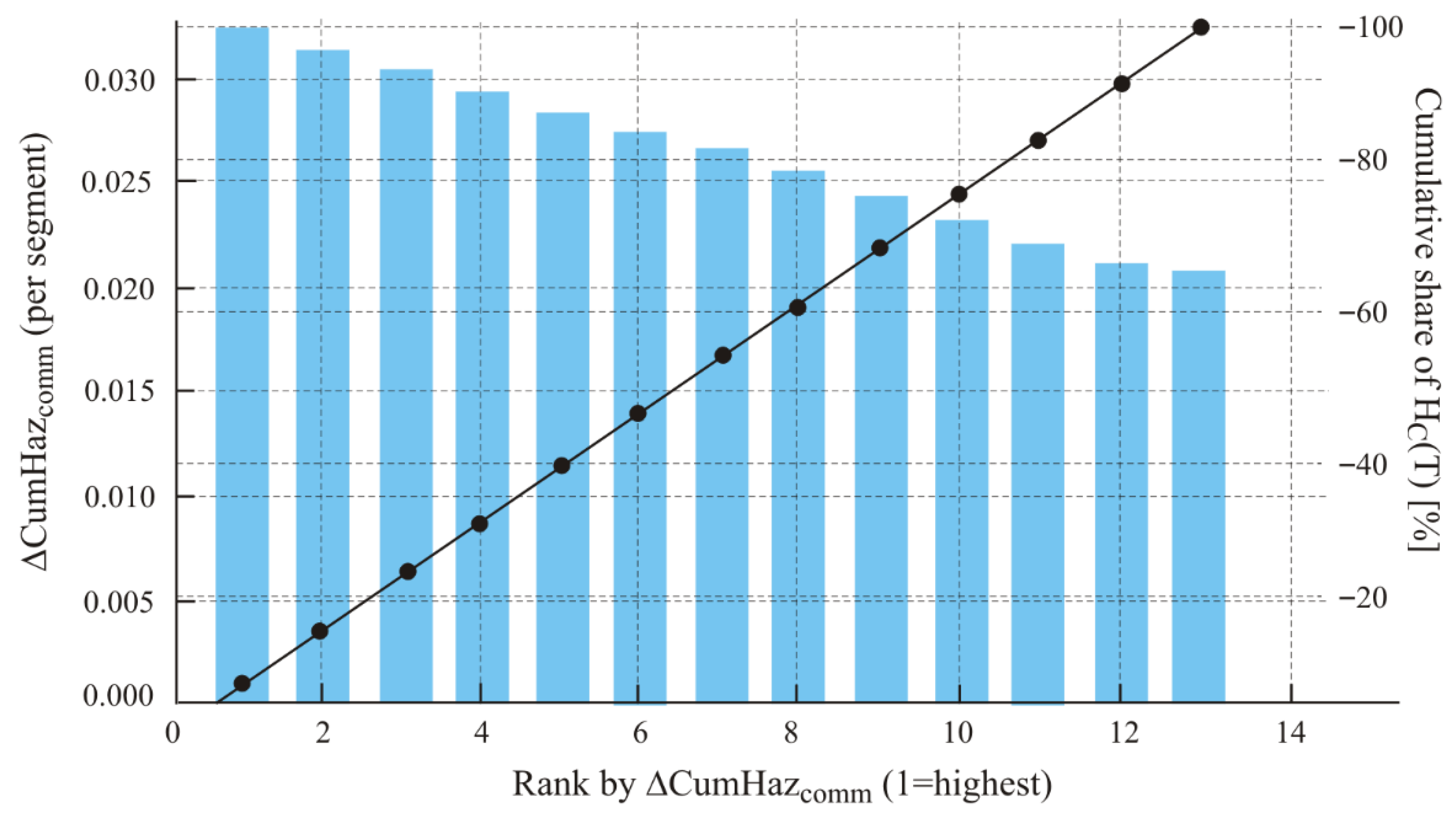
The final dive segment (~342–400 m) accounts for approximately ~27% of the total Comm exposure; this is the most reasonable area to target mitigation measures (communication windows, trajectory adjustments, transmitter power/relay).

The increments for Hull are small and evenly distributed, with no segments requiring immediate action.

Power shows no critical jumps, and the relative contributions from the initial part of the run are minor in absolute terms.

The analysis indicates that the Comm subsystem shapes the end-of-mission risk assessment and is the only one to generate an early-warning signal (Risk ≥ 0.10) about 20 min after the start, at a depth of ~167 m. The Hull and Power subsystems remain in the low-risk zone throughout the analyzed interval, confirming their resilience under the given conditions. The decision threshold α = 0.90 was not reached; therefore, under the adopted assumptions, there were no grounds for abort, and the profile could be continued. The results also highlight the direction for mitigation Comm exposure should be reduced in the final phase of the profile (trajectory adjustment, communication windows, transmitter power/relay). The obtained indicators R_i(T), the time of first warning, and the two mission-level assessments (weighted and independence-based) provide a solid foundation for variant comparisons and sensitivity analyses in the subsequent parts of the study.

These time-to-threshold values (~19 h, ~125 h and ~416 h) follow directly from a constant-rate extrapolation λ_i = H_i(T)/T obtained from the 60 min profile and are, therefore, intended as comparative indicators rather than mission forecasts.

The table shows that Comm has the shortest time to S4 (~6.7 h under the approximate constant λ assumption), while Hull and Power remain far from the critical threshold. Empty rows will be completed once the missing streams are provided (rules and signals in

Table 14. Time-to-state ranking (constant-rate from 60 min profile).

Subsystem	R(T)	t{S2}	t{S3}	t{S4}	Status @ T
Comm	0.291	0.31 h	2.02 h	6.70 h	S2
Hull	0.011	9.98 h	65.6 h	218 h	S0
Power	0.006	17.4 h	114.6 h	381 h	S0
Propulsion	—	—	—	—	—
Control	—	—	—	—	—
Sensors	—	—	—	—	—
Software	—	—	—	—	—

), without the need to expand Table 5.

In the analyzed dataset, the abort decision (α = 0.90) is determined solely by the considered streams Hull/Power/Comm. The remaining subsystems (Propulsion, Control, Sensors, Software) did not influence the abort decision in this analysis, as they were not included in the input data. In other operational profiles, however, their impact may be significant. 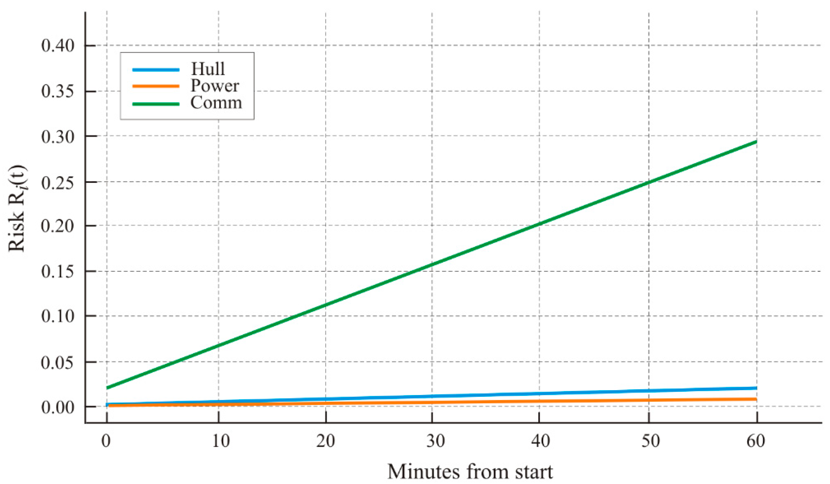The evolution of subsystem risk over the mission timeline is summarized in Figure 6.

Risk trajectories R_i(t) = 1 − exp[−H_i(t)] for Hull, Power, and Comm over the mission timeline. The hazard H_i is accumulated from instantaneous intensities λ_i (units s⁻¹) and Δt steps derived directly from UTC timestamps in Table 5. A clear scale separation is visible: Comm grows steeply and drives the overall mission assessment, while Hull and Power maintain low risk levels. At the end of the profile: R_C(T) ≈ 0.291, R_H(T) ≈ 0.011, R_P(T) ≈ 0.006. This difference identifies Communications as the main reliability limitation under the examined conditions. 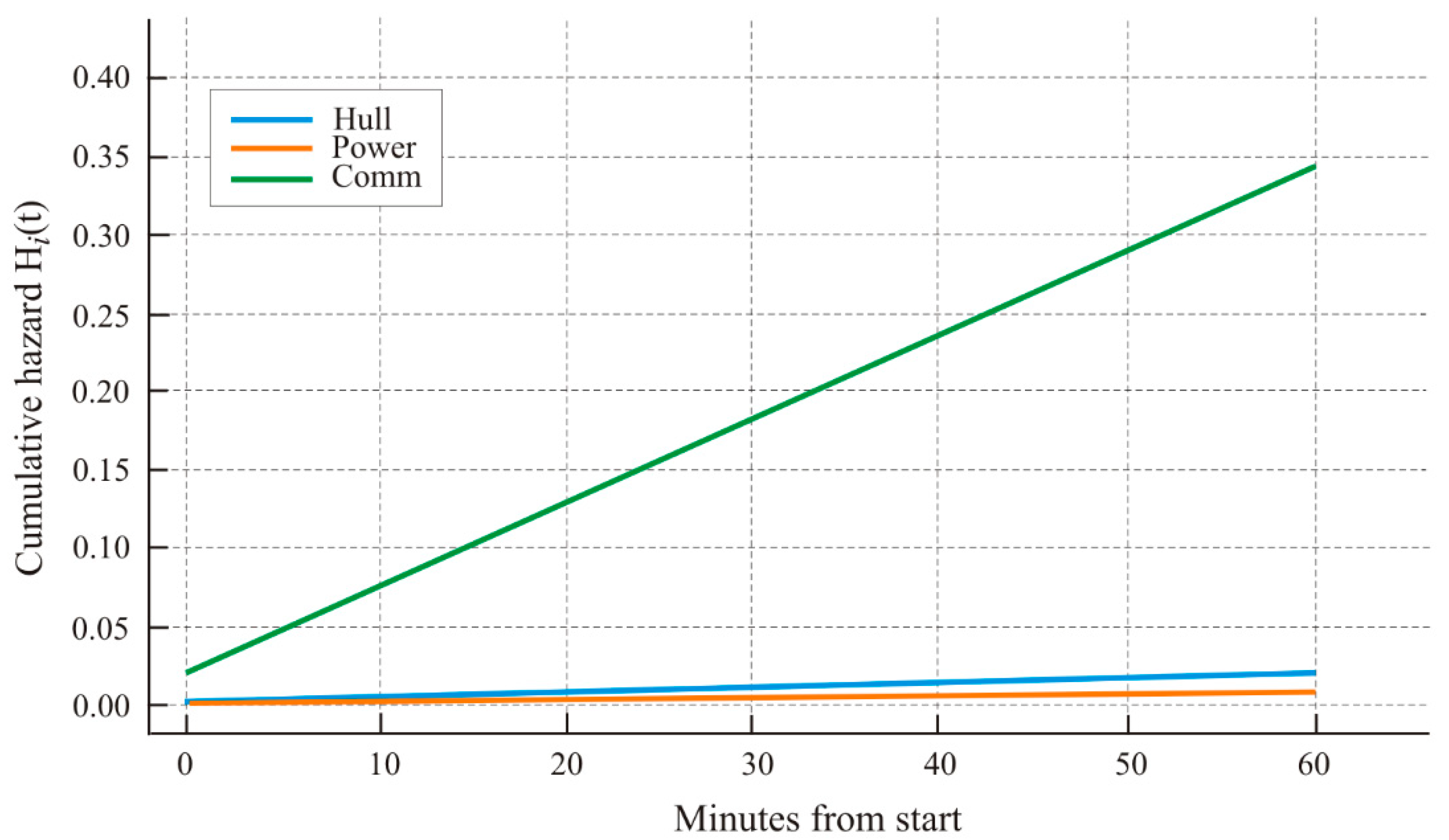The cumulative hazard accumulation for the three subsystems is presented in Figure 7.

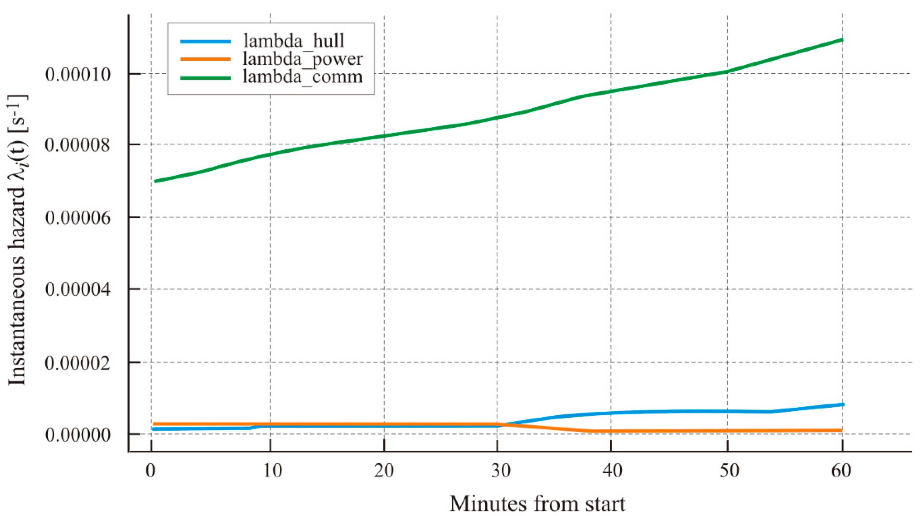
Cumulative hazard H_i(t) = ∑_kλ_i(k) Δt_k for the three subsystem. The curves are monotonic (each segment contributes δH_i = λ_iΔt), and their slope reflects local exposure/conditions. Final values are as follows: H_C(T) ≈ 0.344, H_H(T) ≈ 0.0106, H_P(T) ≈ 0.0060. The change in the growth rate of H_C near the end of the profile correlates with increasing TL_dB and depth. Figure 8 illustrates the instantaneous transition intensities λi(t) computed in 5-minute windows.

Instantaneous intensities λ_i(t) (D6–D8) in 5 min windows. The Y-axis shows transition rates (s⁻¹), and the X-axis shows mission time. λ_C(t) exhibits an upward trend with deteriorating propagation, whereas λ_H(t) and λ_P(t) remain an order of magnitude lowering. These profiles drive the dynamics of H_i(t) and underpin the subsequent threshold plots. The risk trajectories compared against the early-warning and abort thresholds are shown in Figure 9.

Risk trajectories R_i(t) with thresholds α_e = 0.10 (early warning) and α = 0.90 (abort threshold) overlaid. The first exceedance of α_e occurs for Comm after ~20 min at a depth of ~167 m (segment Dk = 5). The decision threshold α is not reached, confirming the feasibility of mission continuation under the analyzed conditions. Figure 10 depicts the dependence of the communication subsystem risk on propagation losses (TLdB).

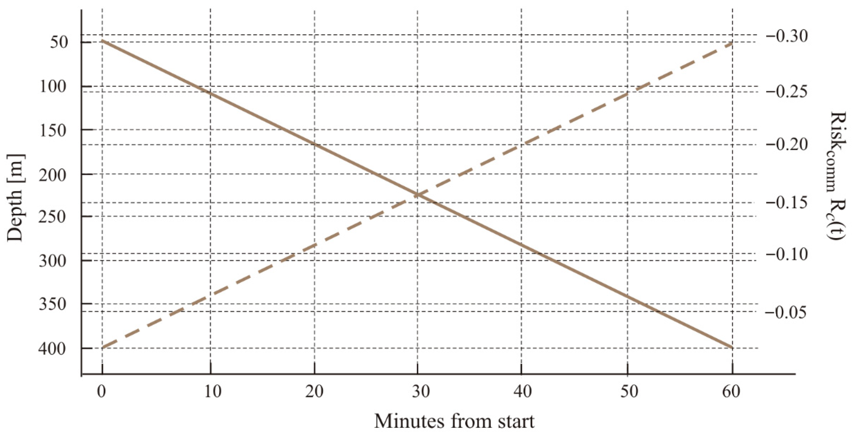
Dependence of R_C on propagation losses (TL_dB), shown pointwise per segment. The relationship is increasing and close to exponential: higher losses shift the risk distribution toward higher levels and shorten the time to thresholds. In practice, this means that communication windows (or trajectory/power/relay adjustments) are the most effective levers for reducing R_C. The relationship between communication risk and depth across the mission is visualized in Figure 11.

Dependence of R_C on depth. The early-warning threshold α_e is reached at ~165–170 m; below this range, communication risk remains low, while above it, the risk increases progressively faster. This aligns with the final descent phase (segments Dk 11–13) and with the Pareto results. Figure 12 provides the Pareto ranking of segment-level contributions to the communication hazard.

Pareto contributions of segments to HC. The largest share comes from the three final descent segments Dk 11–13, accounting together for ~27% of the Comm hazard. These are the natural targets for mitigation (transmission windows, re-trajectory adjustments, power/relay), since any improvement in these segments yields the greatest reduction in risk. Mission-level reliability, aggregated using equal and operational weights, is presented in Figure 13.

Mission-level measures over time $R_M^w\left(t\right)$ (weighted aggregation, shown for both equal and operational weights) and $S_M^{\Pi }\left(t\right){\prod }_i(1-R_i(t\left)\right)$ under the assumption of subsystem independence. Both assessments remain well below the threshold α = 0.90, the difference between the weighting variants reflects operational preferences (greater emphasis on communications lowers the assessment slightly more). 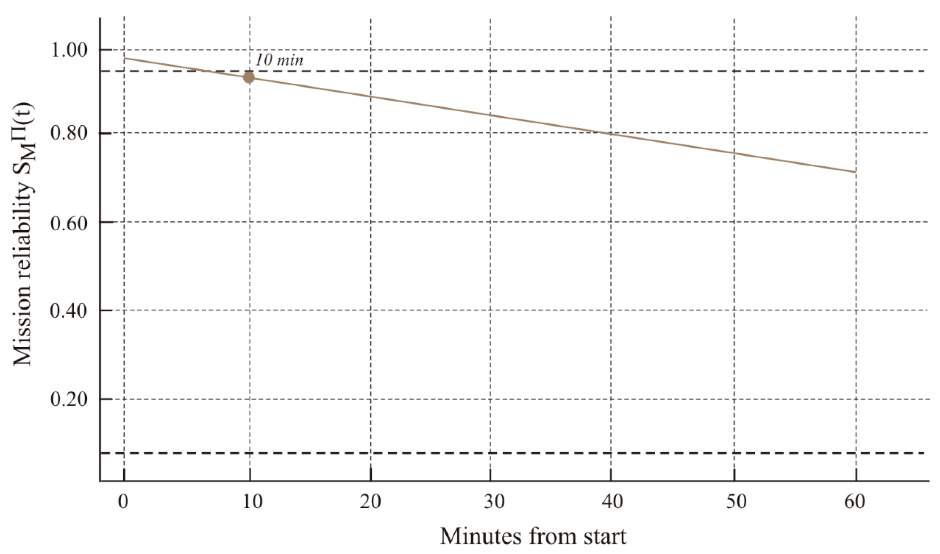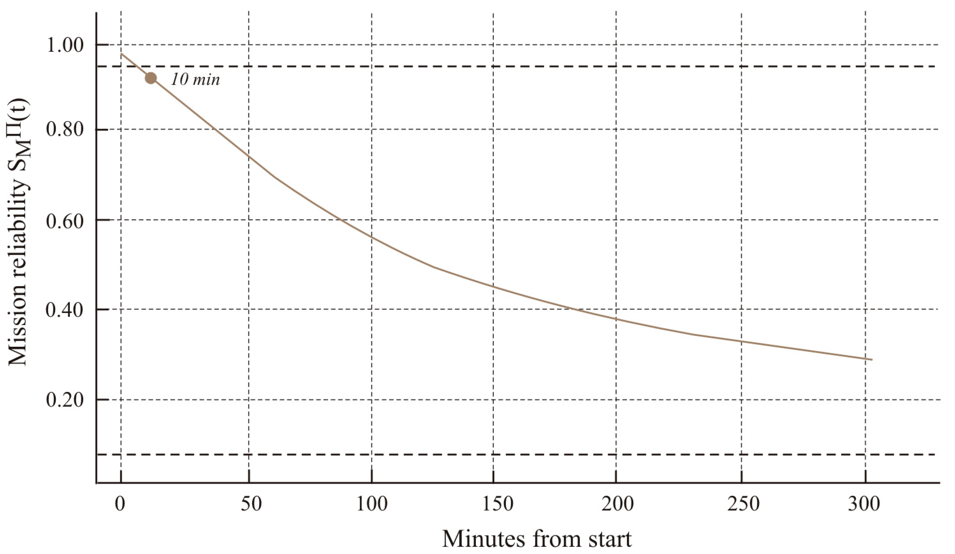Figure 14 shows the extrapolated mission-level reliability curve over a 4-hour operational horizon.

Mission reliability $S_M^{\Pi }\left(t\right)$ over a 4 h horizon, obtained by neutral extrapolation of the 60 min profile (repetition of the ΔH sequence). The curve shows the pure effect of hazard accumulation without any change in the environmental regime and serves as a baseline for comparing variants of mission duration, trajectory, or communication-window policies. 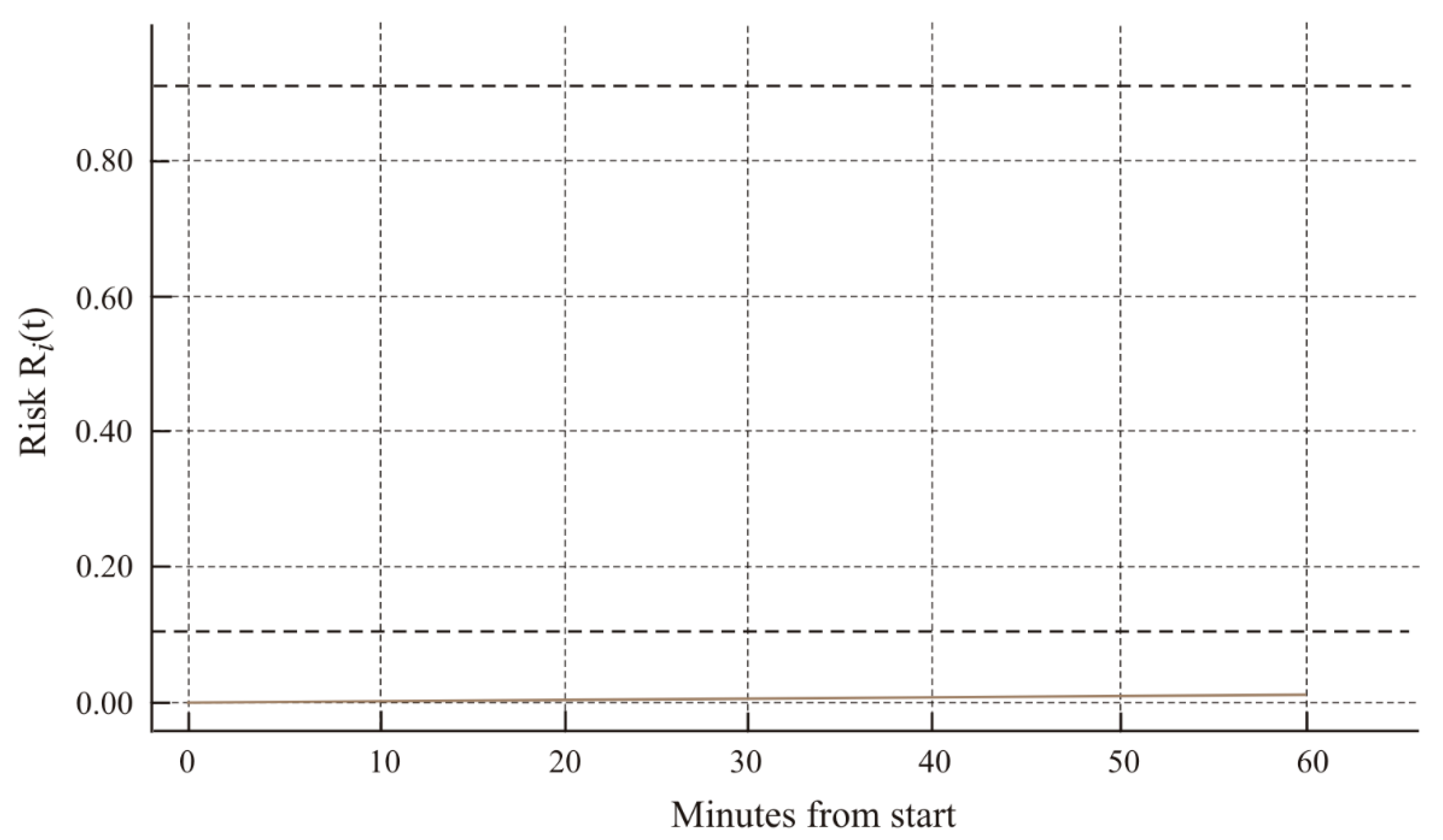The structural-risk trajectory for the Hull subsystem is shown in Figure 15.

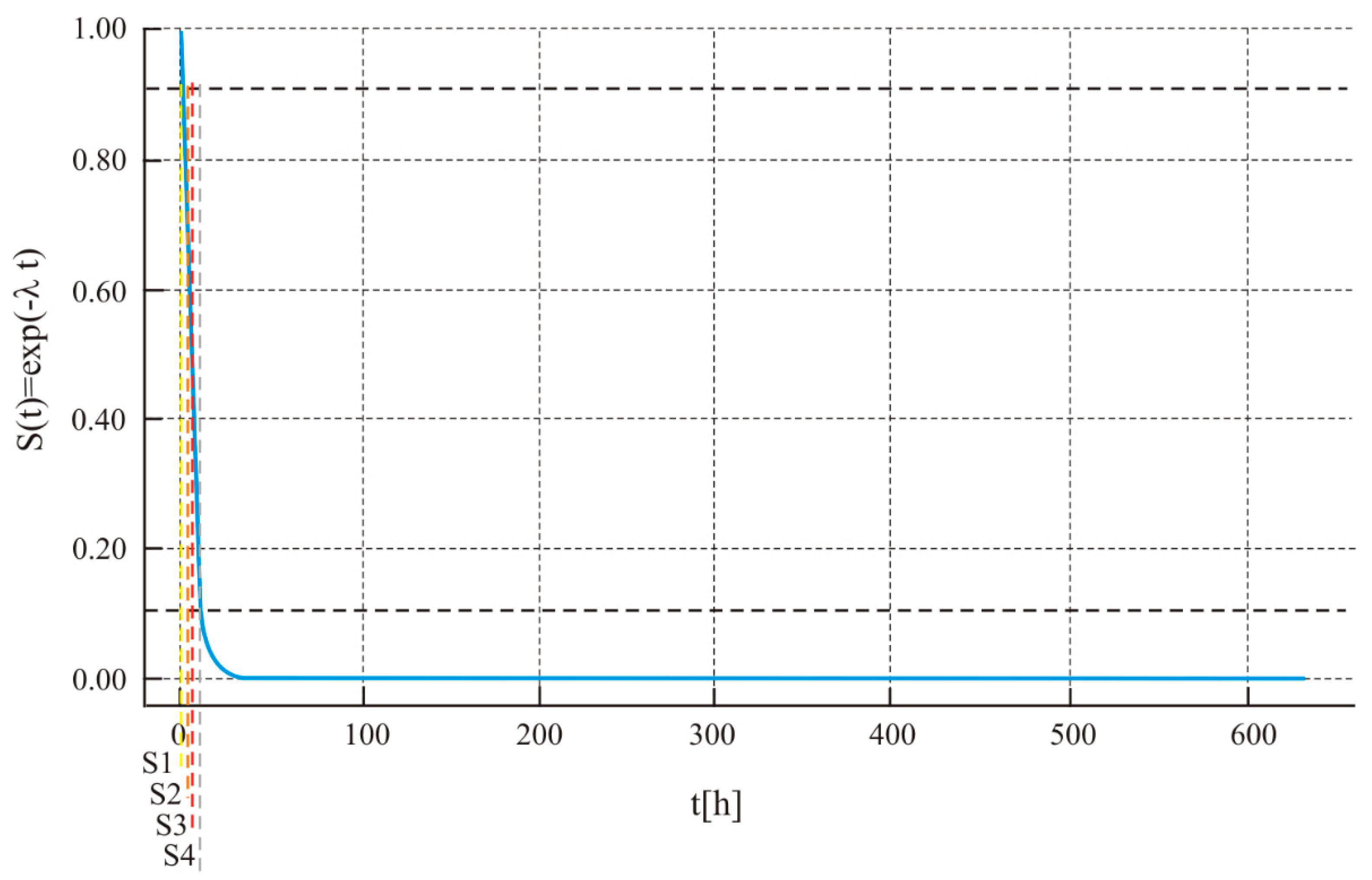
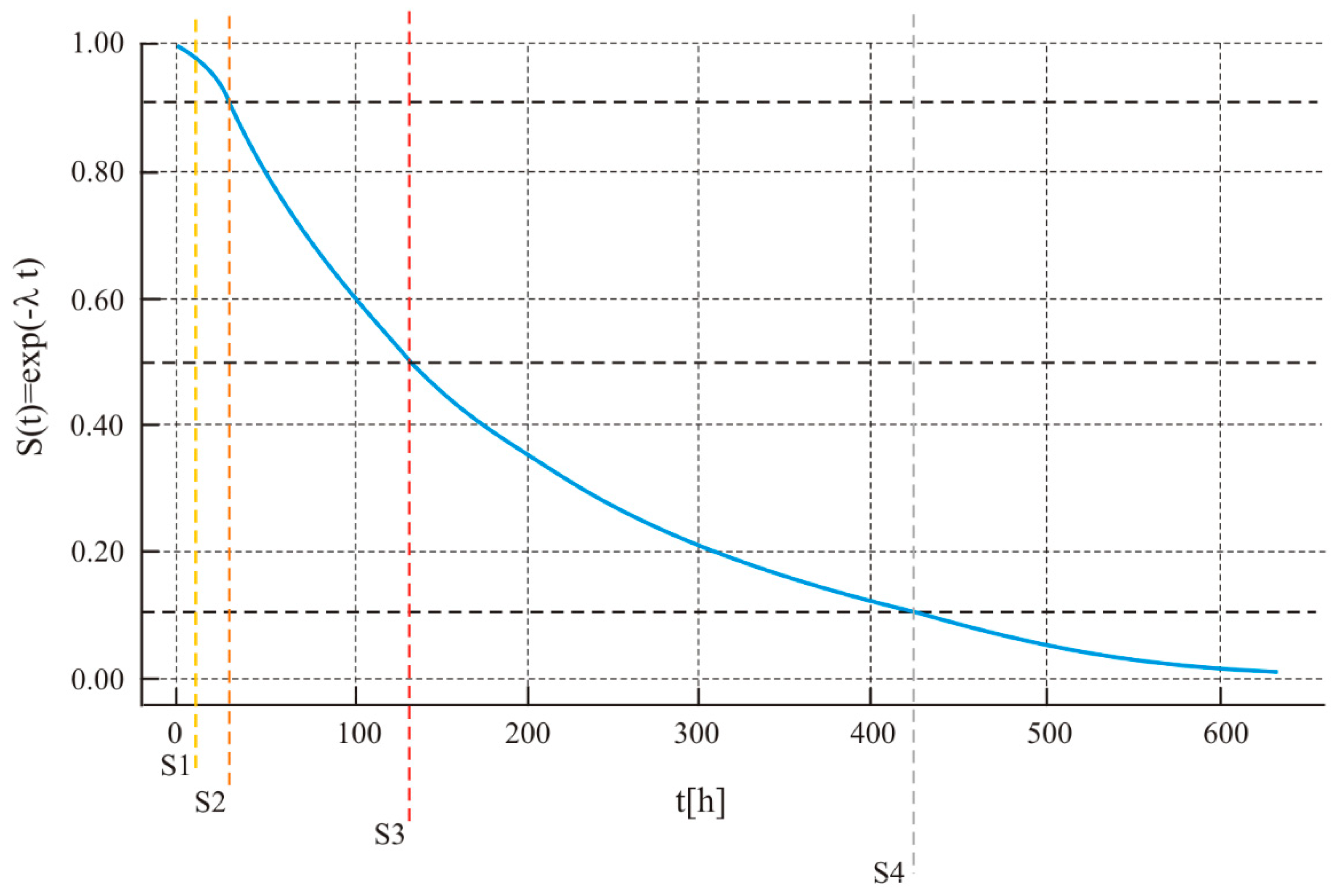
The entire trajectory remains in the S0 zone (below 0.10), with the final R_H(T) on the order of 1%. No signs of escalation are visible in the data (no growth in λ_H), indicating a comfortable structural margin for the analyzed depth and duration. Figure 16 displays the communication-reliability curve S_C(t) together with the S1–S4 threshold markers.

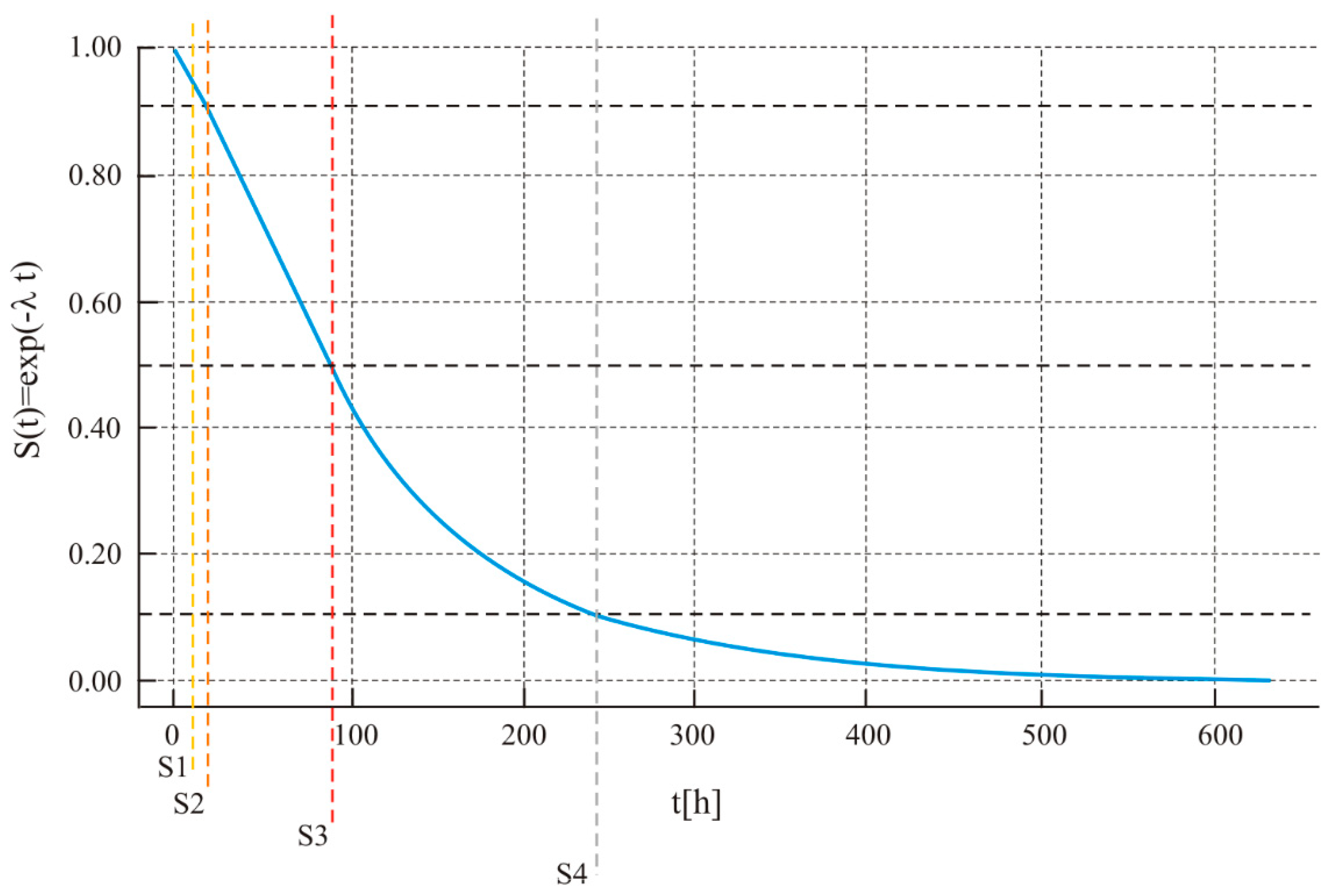
Reliability curve S_C(t) = exp(−λ_Ct) with vertical markers S1–S4. The rate λ_C was estimated from H_C(T)/T (60 min). Characteristic readings: S2 (corresponding to R = 0.10) at ~0.3 h, S3 (R = 0.50) at ~2 h, and S4 (R = 0.90) at ~7 h. The common X-axis scale enables direct comparison of horizons across subsystems; Communications clearly has the shortest time to critical states. The reliability trajectory SH(t) for the Hull subsystem, including S-state markers, is depicted in Figure 17.

The estimated times are on the order of ∼11 h (S2), ∼72 h (S3), and ∼238 h (S4), which confirms that under a 60 min exposure the structural risk remains negligible. The figure serves as a reference point for longer tasks (anchoring duties) or missions at greater depths. Figure 18 illustrates the reliability profile SP(t) for the Power subsystem along with the S-state threshold

The horizons to the thresholds are the longest among the three subsystems: ∼19 h (S2), ∼125 h (S3), ∼416 h (S4). In practice, this means that in this profile, the power system does not constrain the operational decision, but in long drifting missions or under high loads, it is advisable to monitor the R_int trend and the E_res/E_need margin (Figure 18).

6. Discussion

The obtained results form a clear picture of risk exposure for the analyzed MBG-AUV mission. Firstly, the bottleneck is acoustic communication: the cumulative hazard for Comm leads to R_Comm(T) = 0.291 and to an early crossing of the warning threshold R ≥ 0.10 around the 20th minute, at a depth of ~167 m. Secondly, the hard resources (hull/structure and power) remain in the low-risk zone throughout the horizon, with R_Hull(T) = 0.011, R_Power(T) = 0.006. Thirdly, the aggregation method at the mission level is of significant importance: for equal weights of the three subsystems, we obtain $R_M^w$(T) = 0.102, whereas under the independence assumption $R_M^{\prod }$ (T) = 1$- {\prod }_i$(1 − R_i) = 0.302, the difference of 0.10 vs. 0.30 demonstrates that the choice of mission metric (and subsystem weights w_i) must be explicit and agreed to operationally prior to the mission.

In coastal and shelf missions, it is the acoustic channel that degrades most rapidly: rising propagation losses (TL_dB), path geometry, and increasing distance cause SNR to drop; PER/BER to increase; and RTT to extend. These exact signals feed into the communication intensity λ_Comm(t) (column D8) and accumulate hazard at the actual time intervals Δt_k. The parameter ranges of ${\lambda }_i\left(t\right)$ and the effects of environmental drift follow directly from the observed environmental and operational signals and are not imposed arbitrarily; the model, therefore, reflects the actual mission exposure exactly as recorded in the telemetry logs. For Hull and Power, the exposure profile in this mission was mild: the depths and rates of pressure change did not generate escalating leakage risk, and energy reserves did not approach termination regions nor indicate significant aging within the analyzed T. This risk structure aligns with operational practice in AUVs and with numerous reports that links and navigation more often determine mission margins, while structure and energy, when properly designed, rarely constrain short profiles.

From the mission command perspective, the results provide three things: (a) the time of the first warning (here ~20 min), which can be synchronized with a communication window/operational event; (b) subsystem ranking by contribution to risk (Comm ≫ Hull ≳ Power); (c) the numerical state at T, which can be directly inserted into the “continue/abort” decision rule. In practice, mitigations should be directed primarily towards the link: shallower trajectory in the critical segment, correction of communication windows (more frequent/shorter), relay/surface gateway, or higher transmitter power (if the energy budget allows). For Control/Navigation (once these subsystems are included in the full dataset), similar roles are played by decisions about maintaining DVL bottom-lock (altitude above seabed, avoiding sediments). For Power, load profile and monitoring ΔR_int are relevant.

Many field studies with AUVs indicate that the acoustic channel is the most fragile element of the reliability chain, especially in shallow waters and complex bathymetry. The results presented here confirm this intuition quantitatively. At the same time, the applied time-varying (exposure-dependent) hazard and integration over actual Δt intervals move beyond the classical stationary CTMC view and better fit onboard telemetry with UTC timestamps. This translates into interpretability: every number in Table 7, Table 8, Table 9, Table 10, Table 11, Table 12, Table 13, Table 14 and

Table 15. Proposed signals and rules to derive λ/ψ/μ (by subsystem).

Subsystem	Minimal Signals (from Table 4)	Example λi(t)/Proxy	Functional Triggers ψ (Examples)	Recovery μ/Loss ν
Power	V, I, Rint, Tcell, Eres/Eneed	λP = c · exp(β1 · ΔRint/Rint + β2 · T)	ψ0→1: ΔRint/Rint > θR; ψ0→2: rapid drop of Eres/Eneed; ψ0→3: BMS reset at low reserve	μ: stabilization after throttling/load shedding
Propulsion	Ithr, RPM, control demand, hydrodynamic load u	λprop = c · exp(γ1 · asym(Ithr) + γ2 · u)	ψ0→2: thrust asymmetry > θasym; ψ2→3: actuator/ESC saturation > θsat	μ: regain reference, change control mode
Control	depth/heading errors, DVL bottom-lock, IMU drift	λctrl = c · exp(η1 · edepth + η2 · eheading) + penalty when bottom-lock is lost	ψ0→2: bottom-lock loss and growing error; ψ2→3: unstable control for > θ_time	μ1: controller stabilizes/reference recovered
Comm	SNR, PER/BER, RTT, TLdB	λC = c · exp(ξ1 · TLdB) or λC ∝ PER within Δt window	ψ0→3: link blackout (PER > θPER over Δt); ψ0→2: excessive RTT	μ: successful comms window
Sensors	SNR, quality flags, detection metrics	λsens = c · exp(ζ1/SNR)	ψ0→2: quality < θQ (switch to spare sensor)	μ: quality back above θQ
Hull	depth z(t), salinity/stresses S/σ, flooding L	λH = c · exp(α1 · z + α2 · S)	ψ0→3: increasing moisture L > 0; ψ3→4: sharp growth of L	ν: loss of telemetry after T*
Software	watchdog events, resets, TCPU	λ_sw = c · exp(χ1 · TCPU)	ψ0→2: watchdog; ψ0→3: reset cascade	μ: stable uptime > θup

can be directly read on the state graph (Figure 2) and signal map (Table 1 and Table 2).

Two aspects are particularly sensitive:

• Warning threshold α. Changing α shifts the time of the first alarm: a lower threshold triggers earlier (more conservative), a higher threshold later (more tolerant). For this mission, α = 0.10 generated a warning at ~20 min, with α = 0.20, the alarm would shift significantly deeper into the profile. The choice of α\alphaα should depend on tasks (mapping vs. intervention) and acceptable abort costs.
• Weights w_i and aggregation function. Even simple weighting scenarios show Comm dominance: for (w_Comm,w_Hull,w_Power) = (0.5, 0.25, 0.25) we obtain $R_M^w$ $= 0$.150, and for (0.7, 0.15, 0.15) $R_{M }^w$≈ 0.206. Regardless of weight selection, the multiplicative metric $R_M^{\prod }$ gives a clearly higher assessment (0.302) than the weighted average (0.102), which must be explicitly communicated to operators.

The calculations are based on three subsystems (Comm, Hull, Power), as these intensities λ_i(t) were available in data D6–D8. The other four subsystems (Propulsion, Control/Nav, Sensors, Software) are currently described qualitatively and in the factor map.

Calibration of intensities (Table 1) is simplified and does not cover parameter uncertainty; no full Bayesian identification or cross-validation was performed. An independence was assumed in $R_M^{\prod }$, aggregation, whereas actual interdependencies (bottom-lock loss ↔ PER increase) may alter results. A natural extension of the present framework is the explicit modeling of subsystem dependencies, for example, through correlated transition intensities or copula-based risk aggregation, particularly when multi-mission datasets become available. The analysis covers one mission/profile; generalizations require multi-session datasets under varying acoustic and energy conditions. The “no L” variant does not yet include an explicit platform loss model (transition ν: S4→L); in practice, ν should be modeled and reported separately for high-risk profiles.

The presented approach shows that CTMC with exposure-driven intensities and integration over actual Δt effectively captures operational state logic with telemetry. This allows derivation of threshold times (early warning), values R_i(T), and mission aggregates directly from data, without arbitrary averaging over fixed intervals.

Future research directions will include extending the model to all seven subsystems and full calibration of λ_i(t) with exponential models incorporating covariates (depth, TL_dB, temperature, ΔR_int); hierarchical Bayesian identification and uncertainty intervals for H_i(T) and R_i(T); inter-subsystem couplings (Control/Nav↔Comm) and time-dependent returns μ₁(t),μ(t); introduction and calibration of the platform loss arc ν: S4→L with a dedicated decision rule, integration with trajectory planning (risk-aware routing) to control TL_dB exposure and maintain bottom-lock while respecting the energy budget.

For the considered mission profile, communication determines risk assessment and the moment of the first warning, while Power and Hull ensure a comfortable margin. The method (CTMC + Δt from data) provides operational, time-comparable indicators and naturally links them to the S0–S4 graph. Extending it to the full seven subsystems and incorporating uncertainty will enable more formal and defensible “continue/abort” decisions under diverse conditions.

7. Conclusions

The proposed methodology links the state graph S0–S4 with MBG-AUV telemetry through a Markov chain with exposure-driven intensities and integration over actual time intervals Δt derived from UTC timestamps. As a result, the obtained indicators are both interpretable (each change can be assigned to a specific graph arc and mission profile segment) and operational (suitable for direct use in the “continue/abort” rule). In the analyzed 60 min mission profile, the final subsystem risks were R_Comm(T) ≈ 0.29, R_Hull(T) ≈ 0.011, and R_Power(T) ≈ 0.006, and the first warning threshold (αₑ = 0.10) was crossed after ~20 min at a depth of ~167 m. In the analyzed profile, the dominant carrier of risk proved to be acoustic communication; while hull and power maintained low levels of threat, the difference between weighted and multiplicative aggregation shows that the choice of mission metric and subsystem weights must be defined prior to launch and explicitly communicated.

From a theoretical perspective, the key point is that the intensities λ_i(t) are functions of environmental and onboard signals (TL_dB, bottom-lock availability, ΔR_int), other than constant parameters. This formulation strengthens the link between the observed exposure and decision variables, enables reliable estimation of the time of the first warning, and facilitates mission comparisons without arbitrary averaging.

In practice, the mission state assessment procedure involves synchronizing subsystem streams in UTC, performing quality control and unit harmonization, and then mapping data columns to instantaneous transition intensities in accordance with the conventions (D6→λ₃ for Hull, D7→λ for Power, D8→λ₅ for Communications), with the time step Δt directly obtained from successive timestamp differences. These intensities are integrated along the mission–time axis to determine cumulative hazard Hi(t) and risk Ri(t), with parallel monitoring of the first crossing of the warning threshold αe, along with operational context (segment, depth).

For clarity, cumulative risk is obtained by aggregating the exposure increments implied by the time-resolved intensities, following the standard interpretation used in continuous-time reliability models Mission-level assessment is computed in two ways; first, as the weighted average $R_M^w$(t) with predefined weights w_i, and second, as the independence-based estimate $R_M^{\prod }$(t). These values are then compared to thresholds α_e and α, to decide whether to continue, apply mitigation targeted at the dominant subsystem, or abort in accordance with the safety procedure and available return μ.

Operationally, this translates into earlier warnings and precise targeting of mission actions towards managing link exposure (trajectory, transmission windows, possible relay/surfacing), while maintaining a comfortable energy margin without hardware intervention. The methodology is scalable to subsequent profiles and ready for implementation in ground/onboard tools, as all quantities remain notationally consistent with the model in Section 3.

The limitation of this iteration is the lack of calibrated intensities for the four remaining subsystems and the absence of an explicit model for the loss arc ν: S4→L. Extending the framework to Propulsion, Control/Nav, Sensors, and Software in the same formalism and incorporating inter-subsystem dependencies and parameter uncertainty will complete the full reliability picture. Nevertheless, even at this stage, we obtain a measurable, traceable, and operational description of mission risk that supports the planning, execution, and debriefing of MBG-AUV tasks.