Optimization via Genetic Algorithm of the Sandwich Composite Structure for the Racing Car Monocoque

Abstract

The aim of the study was to carry out optimization via genetic algorithm in order to select the best configuration of the sandwich composite structure from which the racing car monocoque is built. The tools used were the static structural analysis by means of the finite element method and multi-objective genetic algorithm implemented in the Ansys Workbench 2024 R1 software. The optimization was carried out to determine the optimal number of layers and orientation of fibers in the sandwich structure. To evaluate the efficiency of the composite structure proposed for the racing car monocoque, two key indicators were employed: Inverse Reserve Factor (IRF) and Total Deformation Load Multiplier (TDLM). The objective function was designed to minimize the overall weight while maintaining the required strength and stiffness of the structure. The results of the conducted analyses demonstrate that the applied optimization via the genetic algorithm method delivers the desired outcomes, meeting the specified design criteria and enhancing the mechanical performance of the monocoque.

1. Introduction

One of the central challenges in the design of sports car frames and skins is the simultaneous achievement of low weight and high mechanical performance. To address this, manufacturers increasingly adopt monocoque structures, where the frame and skin are integrated into a single load-bearing shell. Monocoque solutions made from carbon fiber reinforced polymers (CFRPs) combined with honeycomb sandwich cores provide high stiffness-to-weight ratios and the ability to form complex geometries, making them attractive for motorsport and high-performance vehicles [1,2]. However, high manufacturing costs and limited recyclability restrict their broader adoption outside elite automotive sectors.

The mechanical performance of sandwich composites depends strongly on the selection of constituent materials, ply orientations, and stacking sequences. Optimization is therefore essential to balance weight, stiffness, and strength. Genetic Algorithms (GAs) have proven effective in exploring such complex design spaces by identifying near-optimal laminate configurations while handling non-linear constraints [3]. For instance, recent studies have optimized sandwich structures and layered composites using GAs to improve buckling resistance, stiffness, and crashworthiness [4,5]. A particularly relevant work demonstrated the optimization of honeycomb sandwich composites for lightweight structures using GA, confirming significant performance improvements compared with conventional designs [6].

In addition to single-objective optimization, Multi-Objective Genetic Algorithms (MOGAs) are increasingly applied to trade-off conflicting criteria such as weight reduction versus structural integrity. Researchers have shown that MOGAs can efficiently identify Pareto-optimal frontiers for composite laminates, aiding designers in decision-making [7,8]. Within finite element frameworks, these algorithms allow for systematic evaluation of ply angle and surface distribution, thereby reducing trial-and-error in laminate design.

Although GAs remain popular, alternative metaheuristic approaches—such as Particle Swarm Optimization (PSO), Differential Evolution (DE), and Ant Colony Optimization (ACO)—have also been employed for composite optimization. Several comparative studies indicate that while GA offers robust global search capability, PSO and DE may achieve faster convergence in certain structural optimization problems [9,10]. Benchmarking against these methods helps contextualize the efficiency and accuracy of GA-based approaches. Moreover, advanced optimization paradigms, such as topology optimization integrated with additive manufacturing and hybrid GA–machine learning frameworks, are emerging as promising directions [11,12].

Artificial intelligence (AI) techniques further expand optimization capabilities by enabling accurate prediction of material behavior. Machine learning (ML) and deep learning (DL) models have been successfully trained to predict the stiffness, strength, and failure behavior of composites, thereby reducing the need for extensive prototyping [13,14,15]. These models complement evolutionary optimization by serving as surrogate evaluators of candidate designs.

Despite these advancements, many GA-based studies remain limited to simulation environments without experimental validation or robustness analysis. Uncertainty quantification—accounting for material variability, manufacturing defects, and modeling assumptions—remains an open challenge [16]. As a result, while simulation-driven GA frameworks provide valuable insights, their engineering practicality depends on future integration of uncertainty analysis and physical testing.

In this study, a GA and MOGA framework within ANSYS is applied to optimize honeycomb sandwich monocoques by varying ply orientation and number of surfaces per layer. The approach leverages finite element simulations to evaluate performance and generate optimized designs. By consolidating GA-based optimization with layered composite modeling, this work contributes to ongoing efforts to refine lightweight, high-performance sandwich structures for advanced automotive applications.

2. Composite Component Materials

A sandwich structure is a highly advanced form of composite construction that combines the properties of different materials to achieve optimal mechanical properties with minimal weight. The basic elements of such a structure are two thin but durable pieces of cladding and the core that is located between them. The whole is bonded with resin, which results in a durable and light structure.

2.1. Facing

The outer lining layer is made of carbon fiber, characterized by high strength and rigidity at low weight. Thanks to the use of carbon fiber, much better properties are obtained compared to glass fibers. However, carbon fiber is more expensive and requires a more advanced production process.

Carbon fibers can be divided according to their orientation, density, and the way they are interlaced. The main types of carbon fibers are:

• Unidirectional—all fibers are arranged in one direction only;
• Bidirectional—the fibers are laid in 2 directions at angles of 0° and 90° relative to each other (or ±45°);
• Triaxial—fibers are arranged at 3 different angles, most often 0° and +45°/−45°;
• quadraxial—the fibers are arranged alternately in the directions 0°/90°/+45°/−45° (=135°);
• Quasi-isotropic—the fibers are laid in at least 4 different directions and with a symmetrical structure of layers in relation to the central axis.

Carbon fibers have a density of about 1.6–1.8 g/cm³ and a tensile strength of 3.5–7 GPa. Their modulus of elasticity can range from 230 to 600 GPa, making them ideal for applications that require high rigidity with minimal weight [17].

2.2. Core

The core is the central element of the sandwich structure, which is responsible for its rigidity and bending strength. The core can be made of various materials; in this case, honeycomb is used. Made of aluminum, aramid or composites, the honeycomb core has an excellent strength-to-weight ratio. The honeycomb structure allows for even distribution of loads with minimal material consumption. Honeycomb cores made of aluminum have a density of 0.03–0.1 g/cm³, depending on the wall thickness and cell size. They offer exceptional rigidity, low weight and excellent vibration-damping properties. Honeycomb made of aramid (e.g., Nomex) [18] is lighter than aluminum and has better temperature and fire resistance.

2.3. Resin

The resin serves as a binder that binds the cladding to the core and also strengthens the entire structure. Epoxy resin has excellent adhesion to a variety of materials, high tensile and compressive strength, and good resistance to chemical corrosion. It is characterized by a tensile strength of up to 100 MPa and an elastic modulus of 2.5–4 GPa [19]. Its ability to operate in a wide temperature range (−50 °C to 150 °C and above) and its good chemical resistance make it ideal for applications in harsh environmental conditions.

The material parameters of honeycomb and carbon fiber are listed in

Table 1. Material parameters of honeycomb.

Honeycomb
Density	80	kg/m3
Modulus of elasticity
X, Y	1	Mpa
Z	255	Mpa
Poisson’s ratio
XY	0.49
YZ, XZ	0.001
Tensile stress
X	0	Mpa
Y	0	Mpa
Z	5.31	Mpa
Compressive stress
X, Y	0	Mpa
Z	−5.31	Mpa
Shear
XY	0	Mpa
YZ	1.21	Mpa
XZ	2.24	Mpa

and

Table 2. Material parameters of carbon fiber.

Carbon Fiber
Density	1480	kg/m3
Modulus of elasticity
X	91,820	Mpa
Y	91,820	Mpa
Z	9000	Mpa
Poisson’s ratio
XY	0.05
YZ	0.3
XZ	0.3
Tensile stress
X	829	Mpa
Y	829	Mpa
Z	50	Mpa
Compressive stress
X	−439	Mpa
Y	−439	Mpa
Z	−140	Mpa
Shear
XY	120	Mpa
YZ	50	Mpa
XZ	50	Mpa
Tsai–Wu
Coupling Ratio XY	−1
Coupling Ratio YZ	−1
Coupling Ratio XZ	−1

, respectively.

2.4. Surface Roughness and Entrapped Air (Thermal Implications)

Even when the face sheets and core are perfectly bonded, unavoidable microscale surface roughness at each interface increases the real contact resistance and promotes tiny interfacial air gaps. Both effects raise the effective thermal resistance of the sandwich, creating local hotspots under transient racing loads. Quantitatively, studies of graphene-based thermal interfaces show that reducing the surface roughness (Sq) by ~1 µm can lower thermal contact resistance by about a factor of two, evidence that roughness-induced air gaps dominate the conduction bottleneck at composite interfaces [20,21]. For racing monocoques, this means surface preparation (controlled sanding grit, peel-ply, post-cure polish, clean/prime) is not just structural; it is thermal: smoother, conformal interfaces and low void content improve heat spreading in the skins, stabilize adhesive properties, and limit temperature-driven degradation. In practice, we target low-roughness bonding surfaces and validate void content by standard methods (e.g., ASTM D3171) to ensure consistent thermal/mechanical performance [22,23].

2.5. Experimental Implementation and Correlation

We plan a focused validation program using a monocoque coupon matching the optimized layup (275 × 500 mm panel, 4 CF plies, 10 mm honeycomb). The protocol combines: (1) optical profilometry of facesheet roughness prior to bonding; (2) void/air assessment via digestion-based constituent/void analysis (ASTM D3171) and ultrasonic NDT; (3) guarded hot-plate or transient plane source tests to extract effective in-plane and through-thickness conductivity; and (4) static out-of-plane loading (50 MPa pressure field) with DIC for stiffness and strain-hot-spot mapping. While it is difficult to prove global optimality for multi-objective GA designs, the proposed workflow directly correlates roughness/void metrics with thermal resistance and stiffness, providing a rigorous “simulation ↔ experiment” loop and practical confidence in the improvements over baseline Formula Student sandwich configurations [22,24].

2.6. Orienting Carbon Fibers to Create an Effective Conduction Path

Thermal transport in CFRP sandwiches is strongly anisotropic: in-plane conductivity (along fibers) can be an order of magnitude or more higher than through-thickness conductivity (across plies/adhesive) [25,26,27,28]. For practical heat spreading in a monocoque panel, the conduction path should be aligned with expected heat-flow directions by prioritizing UD plies in those directions (e.g., 0° along the principal heat path). If localized heat extraction through the thickness is needed (battery/bulkhead interfaces), through-plane conductivity can be enhanced with engineered interlaminar networks (e.g., nano-/micro-fillers, vertically aligned short fibers, or thin high-k interlayers), which have been shown to raise through-thickness conductivity without compromising laminate integrity [29,30,31,32]. Representative literature values include in-plane k of ~30–80 W m⁻¹ K⁻¹ for CF-epoxy systems with highly oriented or enhanced fibers, versus 10 W m⁻¹ K⁻¹ through the thickness unless modified; continuous pitch-fiber systems can reach even higher in-plane k when design-appropriate [25,26,27,33]. In short: (1) route heat along UD layers for spreading; (2) add targeted through-thickness conduits where required; and (3) minimize interfacial roughness/voids to reduce contact resistance at bonded joints [20,21,22,23,29,30,31,32].

3. Genetic Algorithm

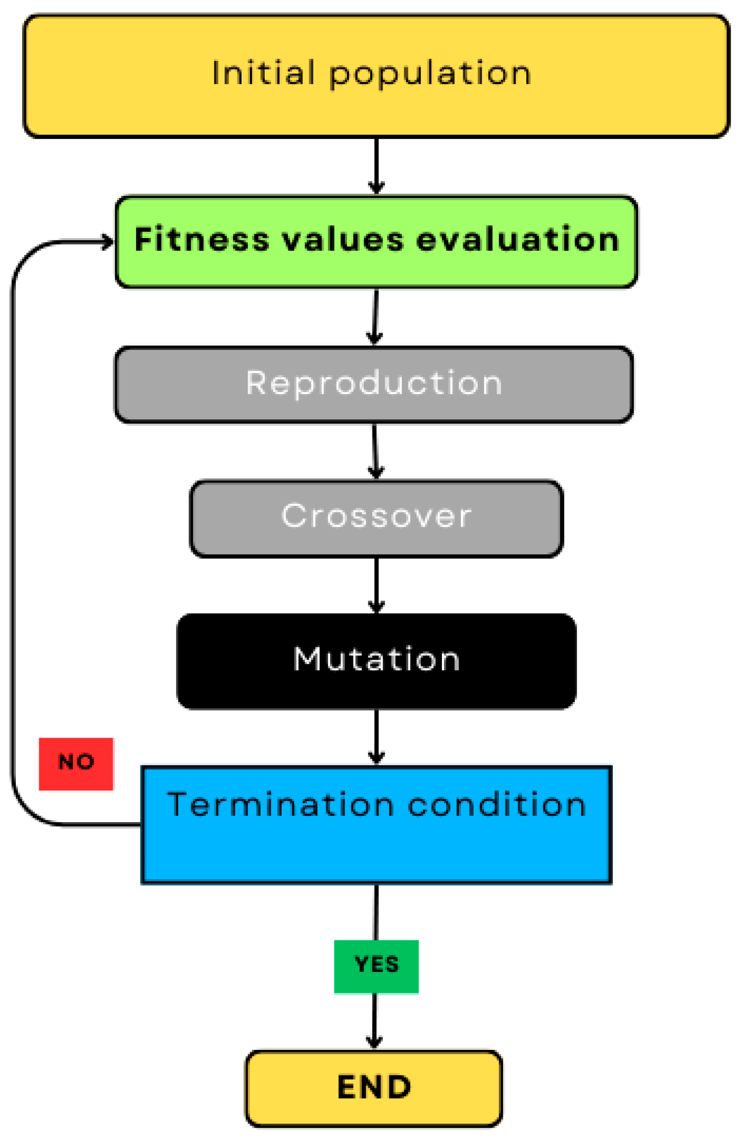
Genetic Algorithms (GAs) are evolutionary metaheuristics inspired by natural selection. They evolve a population of candidate solutions using selection, crossover, and mutation (shown in Figure 1), making them suitable for highly non-linear and discrete optimization tasks [19]. In composite structure optimization, GAs are particularly effective when variables such as ply orientation and stacking sequence are discrete and when the design space contains multiple local optima [3].

In this study, GA was implemented in ANSYS 2024 R1 to optimize honeycomb sandwich composites for monocoque applications. The design variables (P1–P8) include the number of surfaces and orientations for up to four layers, constrained between 30° and 90°. The fitness function was evaluated through finite element analysis (FEA), focusing on maximizing stiffness-to-weight ratio under mechanical performance constraints.

4. Optimization Method

The Multi-Objective Genetic Algorithm (MOGA) implemented in ANSYS [34] extends the classical GA framework to handle multicriteria problems. Unlike single-objective optimization, MOGA seeks to identify multiple solutions along the Pareto front, allowing designers to balance conflicting objectives such as weight reduction and structural integrity [35].

The MOGA in ANSYS is based on the NSGA-II (Nondominated Sorting Genetic Algorithm II), which incorporates controlled elitism, crowding distance, and a fast nondominated sorting scheme [36,37]. Typical crossover and mutation probabilities are 0.7–0.9 and 0.01–0.05, respectively, ensuring both exploration and exploitation of the design space. Convergence is achieved when the Pareto front stabilizes, indicating that further iterations yield no significant improvements.

A diagram of the MOGA is shown in Figure 2. After entering the algorithm parameters, a random initial population is created within the range of defined constraints. This is followed by an iterative process of creating new populations through the use of competitive selection, taking into account the crowding rate and genetic operators such as simple crossing and arithmetic mutation. The typical probability of cross-breeding in genetic algorithms is about 0.7–0.9 (i.e., 70–90%). This means that in each iteration of the algorithm, the crossing operator will be used for about 70–90% of pairs of individuals selected for reproduction. The probability of mutation is usually much lower than the probability of crossing. Typical values are 0.01–0.05 (i.e., 1–5%), which means that only a small percentage of individuals in the population will undergo mutation in each iteration [38]. In an iterative process, convergence is checked. Convergence of the algorithm is achieved when the solutions on the Pareto front stop changing significantly (stability is achieved) and when a certain percentage of Pareto-optimal solutions has been obtained. If these conditions are not met, the algorithm continues to optimize in subsequent steps to further improve the results and look for better solutions.

5. Benchmarking and Comparative Approaches

Although GA and MOGA are widely used, other metaheuristic algorithms—including Particle Swarm Optimization (PSO), Differential Evolution (DE), and Ant Colony Optimization (ACO)—have also been applied to structural and composite optimization. PSO is often favored for its rapid convergence and ease of implementation, whereas GAs remain advantageous for discrete and combinatorial problems such as ply angle and stacking sequence optimization [39,40]. Comparative studies confirm that GA provides robust global search capability, though PSO and DE may achieve faster convergence in certain continuous domains [41,42].

Recent research also highlights the integration of surrogate models, such as neural networks, with evolutionary algorithms to reduce computational costs. Convolutional Neural Networks (CNNs), for example, have been successfully employed to approximate FEA responses, enabling efficient multi-objective optimization of composite shells [8,43,44,45,46].

In this work, GA and MOGA were selected due to their direct availability in ANSYS and seamless integration with FEA. This choice facilitated efficient evaluation of candidate designs under realistic engineering constraints. While benchmarking against PSO, DE, or surrogate-based methods was beyond the present scope, future studies should include such comparisons as well as uncertainty quantification to improve the robustness and practical applicability of optimized sandwich monocoques.

With reference to the scheme shown in Figure 2, cross-breeding in a genetic algorithm involves the exchange of genetic material (i.e., design parameters) between two parents (R1, R2) to generate new individuals (offspring—R1’, R2’). The YES and NO markings determine whether the crossing will be performed for a given pair of parents. YES—means that the pair of parents is undergoing the process of cross-breeding, so new offspring (R1’, R2’) will be generated, which will be created on the basis of the characteristics of the parents. NO—means that crossing will not be applied to this pair, suggesting that the parents (R1, R2) will move on to the next stage unchanged. In this case, the parents without modification will go to the new population (i.e., R1 and R2 remain unchanged). D stands for offspring generated after the crossing process. The offspring (R1’, R2’) are passed on to the mutation process. If the mutation is carried out, mutant offspring (D’) appear. If the mutation is not carried out, the offspring (D) remain unchanged (it is the result of crossing without mutation).

Each P(t) population consists of a set of chromosomes with a certain number. Each chromosome $C_t^j$ in turn, it presents a representation of a given structural form of the system.

$$P\left(t\right)=\left[C_t^1,C_t^2,\dots ,C_t^j,\dots ,C_t^n,\right]$$

(1)

where

• t—population index (iterations),
• n—the number of chromosomes in the population,
• j—chromosome index,
• $C_t^j$—J-th chromosome in population t.

The Meta Model in the form of a Response Surface was used in the optimization. This tool allows one to approximate complex target functions or simulation results using simpler mathematical models. The Response Surface of Genetic Aggregation was used, which allows genetic algorithms to be used to include different response surfaces instead of one, yielding a more diverse and accurate model.

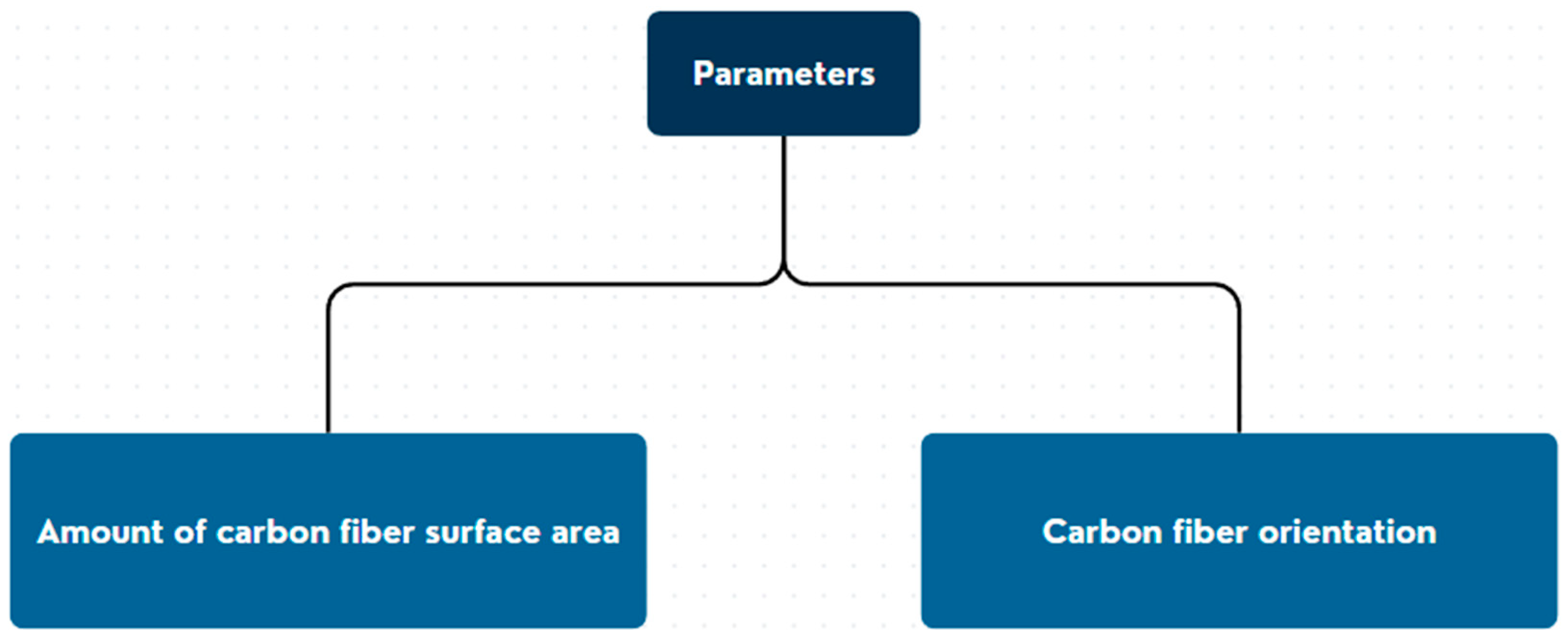
A metamodel is the approximation of the real phenomena by a mathematical model to support computationally expensive simulations. The presented study provides dependencies between geometrical features (Figure 3), the number of fiber layers in each composite layer, the orientation of the carbon fibers in each layer, and the assessment of the stability and deformation of the composite structure.

Figure 3. Project variables.

Figure 3. Project variables.

$$y\left(x\right)\cong \widehat{y}\left(x\right)$$

(2)

where

• y(x)—real response for given x,
• $\widehat{y}\left(x\right)$—approximated response for given x.

The mathematical model can be estimated using three methods. The first one is the analytical method for fundamental physical phenomena, where laws and formulas are well described in the literature. The second method is a passive experiment where the metamodel is based on observed process results. It is applied in cases where the analyzed process cannot be interrupted or influenced. The metamodel is obtained by correlation analysis and statistical tests. The third method is active experiment planning, the so-called design of experiments, where output parameters are evaluated for defined cases. This method can be stationary (all cases defined at the beginning of the experiment) or non-stationary (the first set defined, and the next set of input parameters driven by results from the previous set) [38].

In the article, the stationary design of the experiment method and the applied metamodel with the genetic aggregation response surface approach are used. The model can be written using a weighted average of different metamodels:

$${\widehat{y}}_{ens}\left(x\right)={\sum }_{i=1}^{N_m}{w}_i{\widehat{y}}_i\left(x\right)$$

(3)

where

• ${\widehat{y}}_{ens}$—prediction of the ensemble,
• ${\widehat{y}}_i$—prediction of the i-th response surface,
• N_m—number of metamodels used, Nm ≥ 1,
• w_i—weight factor of the i-th response surface.

The weight factors need to satisfy the following equation:

$${\sum }_{i=1}^{N_m}{w}_i=1\wedge w_i\ge \mathrm{1,1}\le i\le N_m$$

(4)

To find the best weight factors, the algorithm minimizes the root mean square error (RMSE) and predicted sum of squares (PRESS) as reported by Equations (5) and (6), respectively.

$$RMSE\left({\widehat{y}}_{ens}\right)=\sqrt{{\displaystyle \frac{1}{N}}{\sum }_{j=1}^N{\left(y\left(x_j\right)-{\widehat{y}}_{ens}\left(x_j\right)\right)}^2}$$

(5)

$${PRESS}_{RMSE}\left({\widehat{y}}_{ens}\right)=\sqrt{{\displaystyle \frac{1}{N}}{\sum }_{j=1}^N{\left(y\left(x_j\right)-{\widehat{y}}_{ens,-j}\left(x_j\right)\right)}^2}$$

(6)

where

• ${\widehat{y}}_{ens-j}\left(x\right)={\sum }_{i=1}^{N_m}{w}_i{\widehat{y}}_{i-j}\left(x\right)$—estimation of the metamodel ensemble constructed excluding the j-th design point,
• $x_j$—design point jth,
• $y\left(x_j\right)$—output parameter value at xj design point,
• ${\widehat{y}}_{i-j}\left(x\right)$—prediction of the metamodel constructed without the j-th design point,
• N—quantity of design points.

6. Defining the Optimization Task

The optimization task is to find the optimal number of fiber layers in the individual composite layers and the orientation of the fiber while maintaining the minimum value of structure deformation and the failure coefficient. The input parameters are the number of fiber layers (from 1 to 3) in each composite layer and the orientation of the carbon fibers in each of the 3 layers. The first parameter of the task, referring to the number of layers of the fiber, is therefore a discrete parameter—the number of layers from 1 to 3 has been defined. The second parameter of the task, relating to the orientation of the fibers, takes continuous values in the angle range from 30 to 90 degrees (Figure 3). A higher number of fiber layers can increase the strength and stiffness of the structure, but it also translates into more weight and higher production costs.

The set of design variables in a genetic algorithm is stored in the form of chromosomes Ci (7). In the optimization process, the algorithm strives to find the optimum global target function FC (8), which boils down to finding the most suitable chromosome for a defined set of criteria (9,10).

$${\mathrm{C}}_{\mathrm{i}}={\mathrm{x}}_1, {\mathrm{x}}_2,\dots$$

(7)

where

• n—number of design variables,
• $x_i$—value of the i-th variable in the allowable range of the design variable ${\left[x_i\right]}_{min}<x_i<{\left[x_i\right]}_{max}$,
• ${\left[x_i\right]}_{min}$—minimum value of the design variable,
• ${\left[x_i\right]}_{max}$—maximum value of the design variable.

For the analysis of the layered composite material, two criteria were taken into account in the form of stability coefficients f1 and failure coefficients f2. Our goal was to achieve a failure rate above 1 and a stability index below 1 (Equations (10) and (11)).

$$Fc\left\{\begin{array}{c}\underset{Ci}{min}{f}_1\left(X_1,X_2\right)\left(f1<1\right)\\ \underset{Ci}{max}{f}_2\left(X_1,X_2\right)\left(f2>1\right)\end{array}\right.$$

(8)

where

• $f_1,f_2$—function member functions F_C,
• $x_1$—design variable related to the number of layers of the fiber (discrete variable),
• $x_2$—design variable related to the orientation of the fiber (continuous variable),
• $f_1$—Inverse Reserve Factor (IRF) for the stability index of a material before deterioration,
• $f_2$—Total Deformation Load Multiplier (TDLM) describing the degree of deformation of the structure under load.

Inverse Reserve Factor (f₁)

This result type is an inverse margin to the Safety Factor. The failure load can be defined as the load value divided by the IRF. The reserve factor indicates margin to failure.

The applied load multiplied by the reserve factor gives the failure load:

$$RFxFapplied=F_f$$

(9)

Reserve factor values greater than one indicate positive margin to failure, and values less than one indicate negative margin. The values of reserve factors are always greater than zero.

The critical values of reserve factors lie between zero and one, whereas the non-critical values range from one to infinity. Whether the results are shown in numeric form or as contour plots, the non-critical values tend to be emphasized in comparison to critical values. Therefore, the inverse reserve factor is often preferred in practical use:

$$f1={\displaystyle \frac{1}{RF}}$$

(10)

The non-critical values range from zero to one, and the critical values from that on [13].

Total Deformation Load Multiplier

In finite element analysis (FEA), including simulations in ANSYS, the load multiplier (f₂) represents the scaling factor of the applied load P0 at which the structure reaches a critical state (e.g., failure or buckling). The mathematical formula is:

$$f2={\displaystyle \frac{P_{critical}}{P0}}$$

(11)

where

−

f₂ is the load multiplier,

−

Pcritical is the load at which failure or significant non-linear deformation occurs,

−

P0 is the initial applied load in the simulation.

In ANSYS, the Total Deformation Load Multiplier is calculated through iterative simulations, where the applied load, in this case, 50 MPa, is gradually scaled. The simulation stops when the structure reaches its critical load limit, where non-linear effects dominate, such as yielding, plastic deformation, or buckling [16]

Fiber orientation refers to the angle at which the fibers are aligned relative to the main axis of the structure. This parameter is crucial for determining the mechanical properties of the composite, such as tensile strength, stiffness and resistance to damage.

7. Optimized Model

A model with dimensions of 275 × 500 mm, with a fiber thickness of 0.22 mm and a honeycomb core of 10 mm, which is a section of the monocoque structure, has been optimized. The structure is fixed around the entire circumference and loaded perpendicular to the surface with a pressure of 50 MPa. Figure 4 shows the sandwich structure under analysis, consisting of 4 layers of carbon fiber and 1 layer of honeycomb.

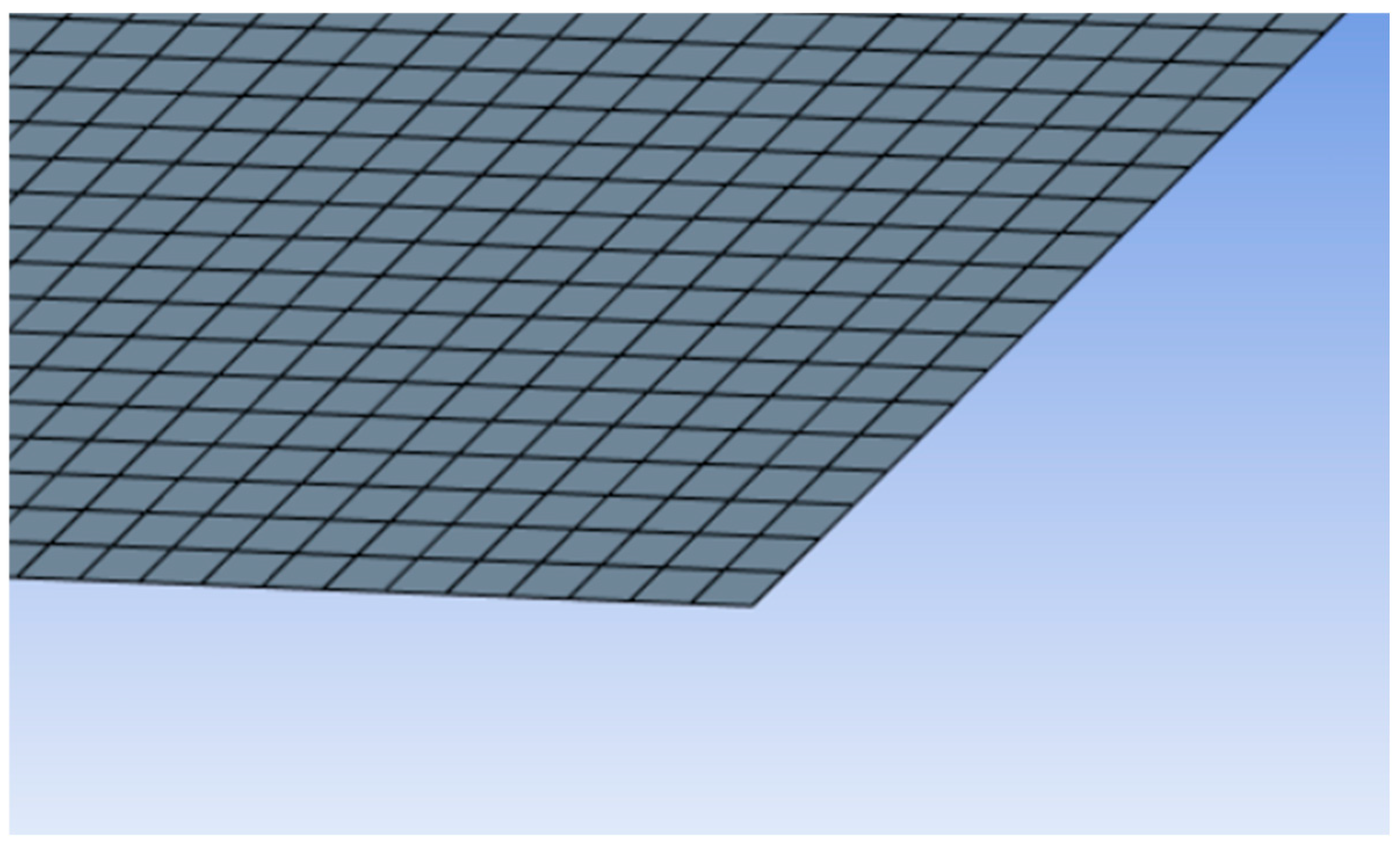
The model was discretized using hex-dominant finite elements with a linear shape function (shown in Figure 5). The mesh is mainly composed of cubic elements, which are preferred for their numerical efficiency and computational accuracy, especially in mechanical and thermal analysis. Hex dominants are often used in FEM analyses where precise results are required, e.g., in mechanical models of composites, in deformation simulations, and in tasks requiring high-quality representation of stresses and strains in sandwich materials.

8. Composites in the Finite Element Method

One of the most commonly used criteria for evaluating the strength of composites in FEM [17] is the Tsai–Wu criterion. This criterion is crucial for predicting composite failure under multiaxial stress states and takes into account the anisotropy of the material, which makes it extremely useful for finite element analyses.

The Tsai–Wu failure criterion for a 2D state plane stress (σ₃ = 0, τ₁₃ = 0, τ₂₃ = 0) is expressed as:

$$F_1{\sigma }_1+F_2{\sigma }_2{2F}_{12}{\sigma }_1{\sigma }_2{F}_{11}{\sigma }_1^2{F}_{22}{\sigma }_2^2{F}_6{\tau }_{12}{F}_{66}{\tau }_{12}^2=1$$

(12)

The material strength parameters of the lamina determine the coefficients Fij of the orthotropic Tsai–Wu failure criterion, which are obtained through experiments. These coefficients are calculated using the following formulas [39]:

$$F_1=\left({\displaystyle \frac{1}{X_1^T}}-{\displaystyle \frac{1}{X_1^C}}\right),F_2=\left({\displaystyle \frac{1}{X_2^T}}-{\displaystyle \frac{1}{X_2^C}}\right),F_{12}={\displaystyle \frac{-1}{2}}\sqrt{{\displaystyle \frac{\frac{1}{X_1^T\ast X_1^C}\ast 1}{X_2^T\ast X_2^C}}},$$

(13)

$$F_{11}={\displaystyle \frac{1}{X_1^T{X}_1^C}},F_{22}={\displaystyle \frac{1}{X_2^T{X}_2^C}},F_6=\left({\displaystyle \frac{1}{X_{12}^T}}-{\displaystyle \frac{1}{X_{12}^C}}\right),F_{66}={\displaystyle \frac{1}{X_{12}^T{X}_{12}^C}}$$

(14)

where

• X^T₁—tensile material strength of laminate along fiber direction,
• X^C₁—compressive material strength of laminate along fiber direction,
• X^T₂—tensile material strength of laminate transverse to fiber direction,
• X^C₂—compressive material strength of laminate transverse to fiber direction,
• X^T₁₂—positive shear strength of laminate,
• X^C₁₂—negative shear strength of laminate (the solver considers it equal to the positive shear strength).

The stress state of the lamina calculated by the program is described by the components σ₁, σ₂, and τ₁₂,

• where
• σ₁—laminate stress along fiber direction,
• σ₂—laminate stress transverse to fiber direction,
• τ₁₂—laminate shear stress.

9. Optimization

Starting to define the optimization task in Ansys, the input parameters in the form of 4 composite layers and the possible fiber orientations for each of the four layers were defined.

Table 3. Definition of variables and constraints on discrete and continuous variables for individual composite layers.

P1—Layer 1—number of surfaces	1, 3
P2—Layer 1—Layer orientation	30–90 deg
P3—Layer 2—number of surfaces	1, 3
P4—Layer 2—Layer orientation	30–90 deg
P5—Layer 3—number of surfaces	1, 3
P6—Layer 3—Layer Orientation	30–90 deg
P7—Layer 4—number of surfaces	1, 3
P8—Layer 4—Layer Orientation	30–90 deg

shows the accepted limits on discrete and continuous values for the number of carbon fiber layers and fiber orientation, respectively.

The optimization assumes minimizing the IRF value and maximizing the TDLM value.

Figure 6 shows a graph generated by the Design of Experiment module showing the analysis capabilities obtained in the optimization process, taking into account the influence of the values of design variables from P1 to P8 on the IRF and TDLM values (mapped as parameters P10 and P11, respectively).

The following graphs present the resulting stability coefficients (IRFs). These graphs have been selected from many generated by the algorithm because they show the largest differences in the values of the coefficients for different configurations.

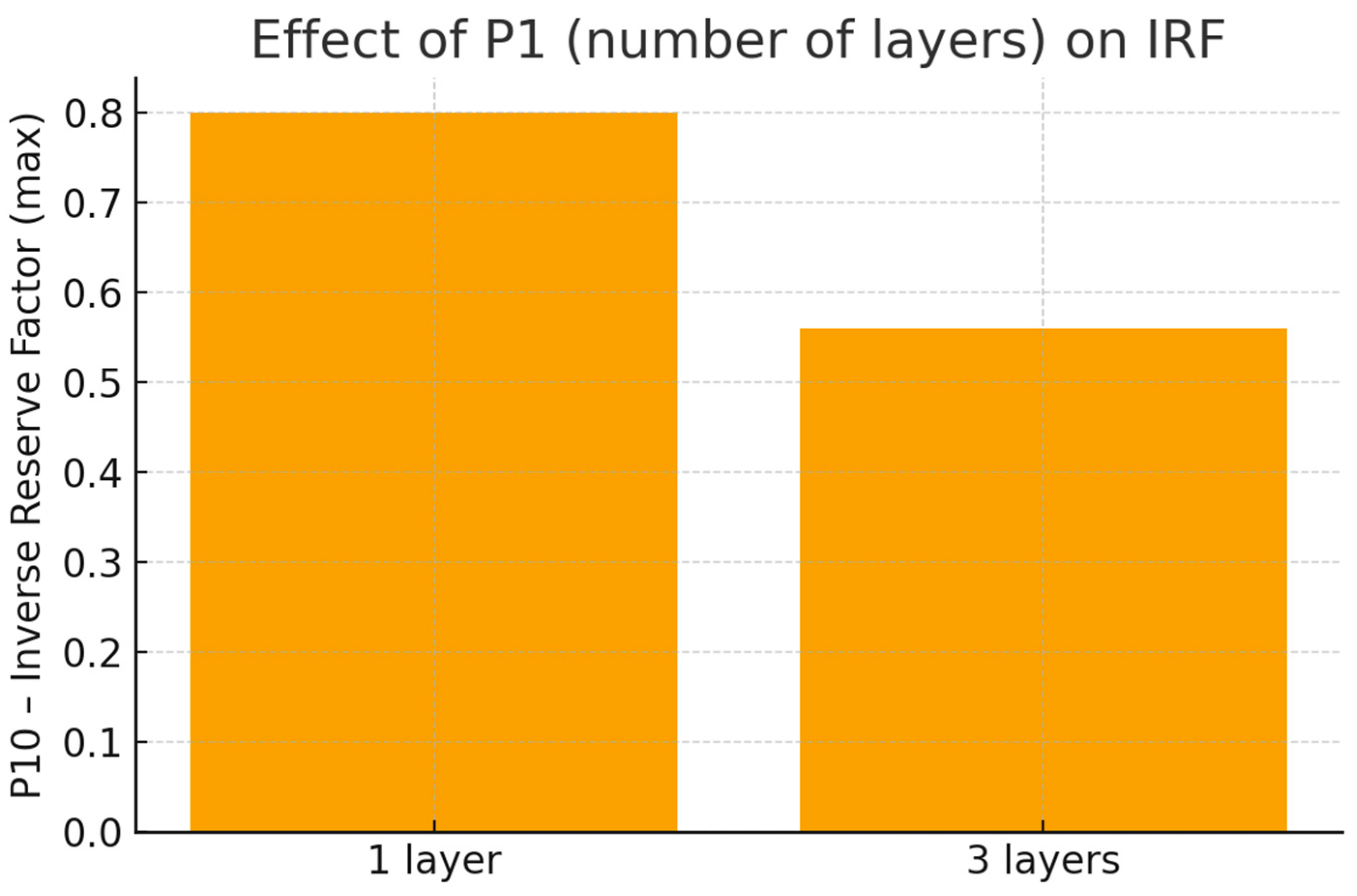
Chart P1—ModelingPly.1.number_of_layers (Figure 7), where the horizontal x-axis represents the number of layers for the first layer named ModelingPly.1. The vertical y-axis represents the maximum value of IRF. For a value of 3 on the x-axis (number of layers = 3), the corresponding value on the y-axis is relatively low, at about 0.55. In contrast, for a value of 1 on the x-axis (number of layers = 1), the value of the Inverse Reserve Factor is much higher, close to 0.8. This means that the configuration for 3 layers has a greater safety headroom than a single layer.

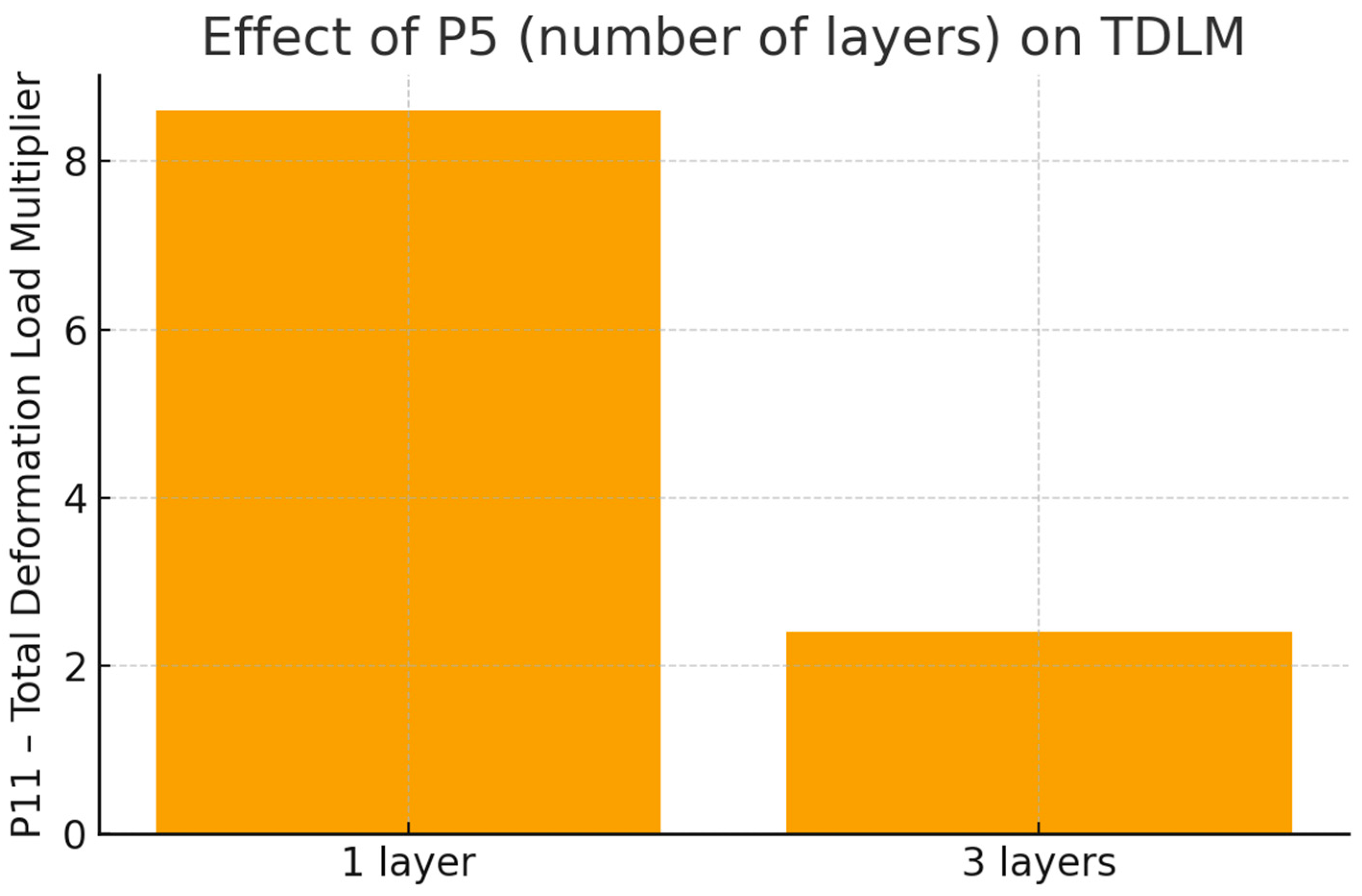
The Figure 8 below shows a comparison of the effect of the number of fiber layers on the TDLM value for layer 3. The horizontal x-axis presents values for the number of layers, while the vertical y-axis presents values for the coefficient. The graph shows that for the 3rd layer, one fiber surface is more advantageous than three.

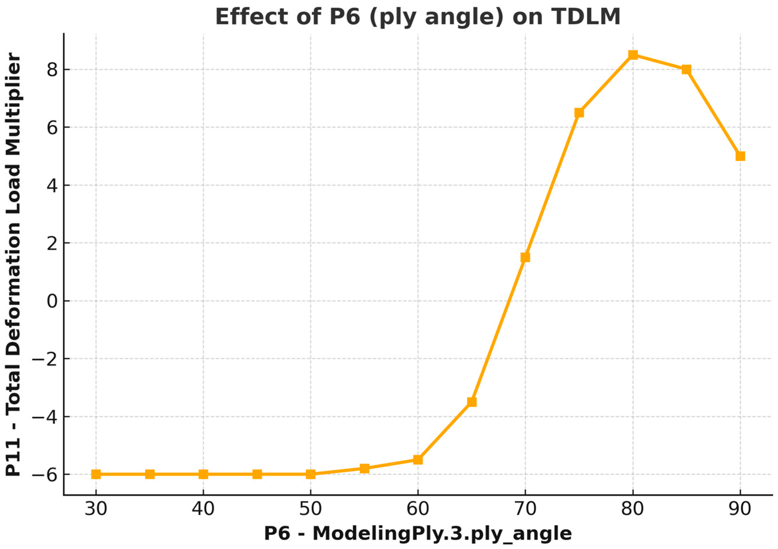
Figure 9 shows the response diagram, for example, configurations and the resulting values of the destruction factors. The x-axis (P6—ModelingPly.3.ply_angle) represents the orientation of the fibers (ply angle), which varies from 30 to 90 degrees. The vertical axis represents the TDLM value. The value of the coefficient begins to increase rapidly, reaching its peak at an angle of around 80 degrees, where it reaches a maximum value of about 9.

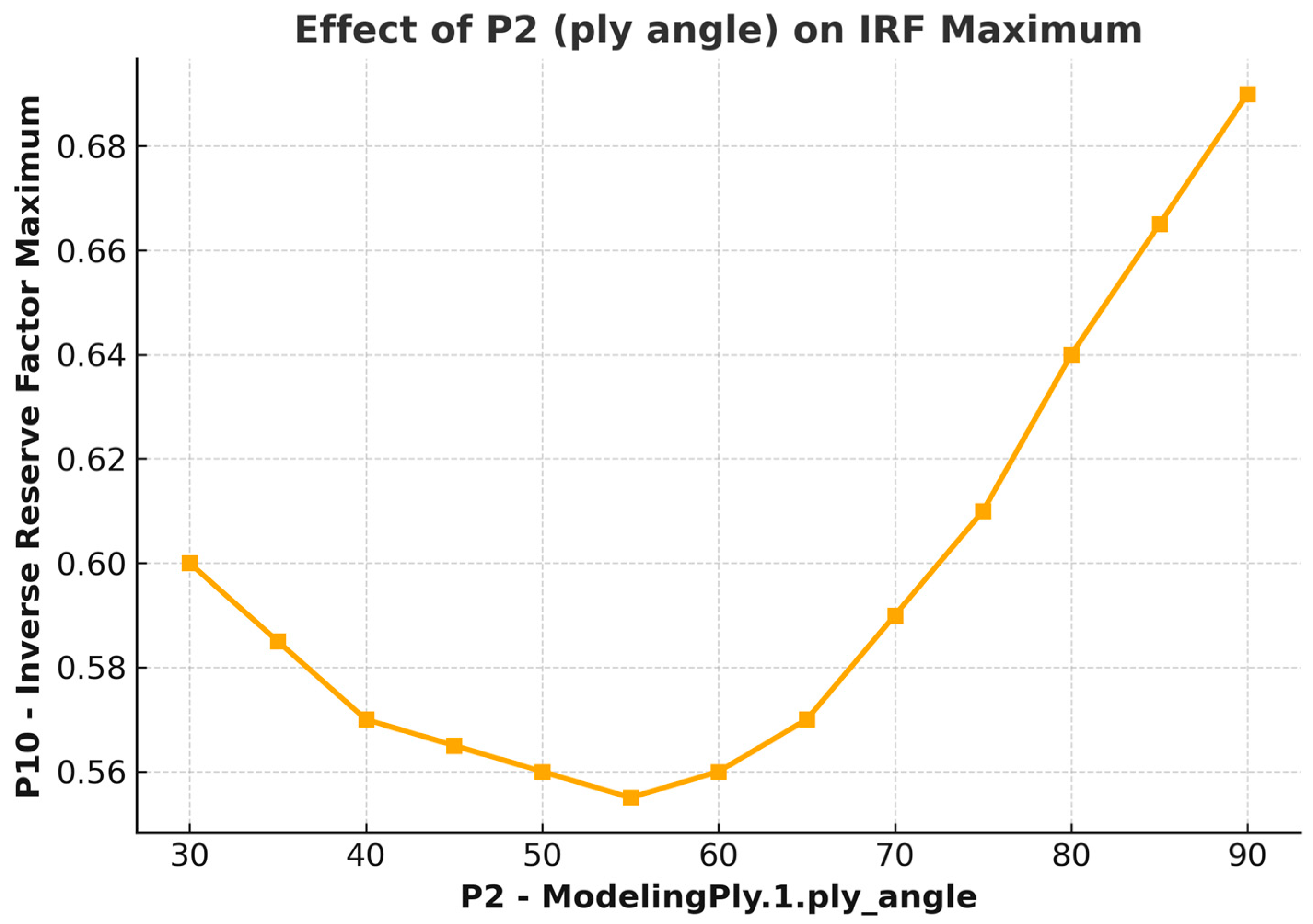
The Figure 10 shows the values of the stability factor due to the orientations of the carbon fibers.

With the help of the MOGA, optimization was carried out to determine the best orientation and amount of carbon fiber for each of the four layers. Results are shown in

Table 4. Optimization output parameters.

	Candidate No. 1	Candidate No. 2	Candidate No. 3
P1—Layer 1—number of surfaces	3	3	3
P2—Layer 1—Layer Orientation	36.711	40.564	49.384
P3—Layer 4—number of surfaces	3	3	3
P4—Layer 4—Layer Orientation	33.09	41.511	32.219
P5—Layer 3—number of surfaces	1	1	1
P6—Layer 3—Layer Orientation	61.213	65.352	46.112
P7—Layer 2—number of surfaces	3	3	3
P8—Layer 2—Layer Orientation	64.97	71.314	71.937
P10—Inverse Reverse Factor	0.572	0.582	0.573
P11—Total Deformation Load Multiplier	1.003	1.001	1.029

.

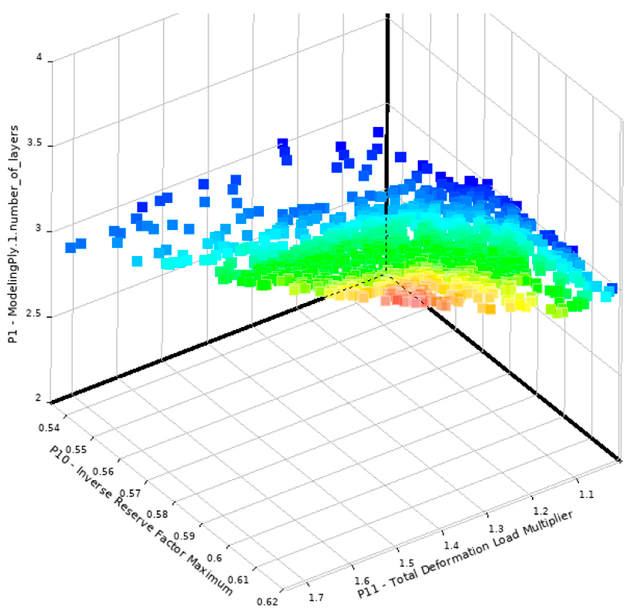
In addition, during the optimization via genetic algorithm, the algorithm generated 56 Pareto Fronts. The three-dimensional graph on Figure 11 shows the data of the fifty-sixth Pareto front, obtained during optimization via genetic algorithm. The x-axis (P1_1) represents the TDLM, the y-axis (P10) is the IRF maximum, and the z-axis (P1_ModelingPy_1_number_of_layers) refers to the number of fiber areas for the first layer of the model. The colors on the chart represent the distribution of values that can be interpreted as an optimization function. The color scheme can represent the level of fitness of solutions in the context of multicriteria optimization. Red and yellow may suggest regions with a worse fitness value, i.e., less optimal solutions. The green color represents more medium solutions. Blue shades, especially darker ones, may indicate the most optimal solutions [36].

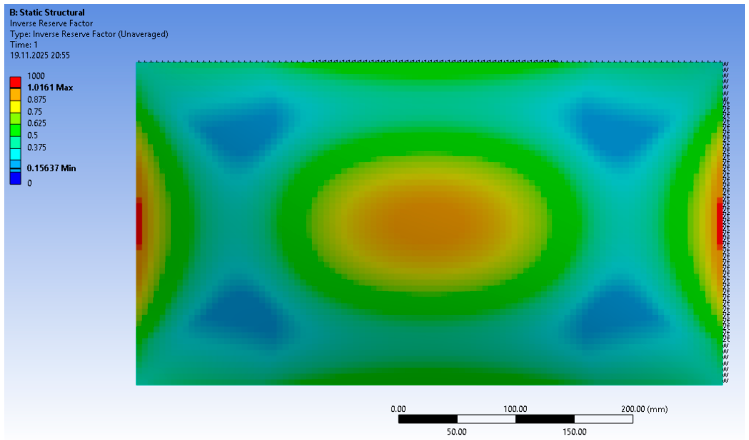
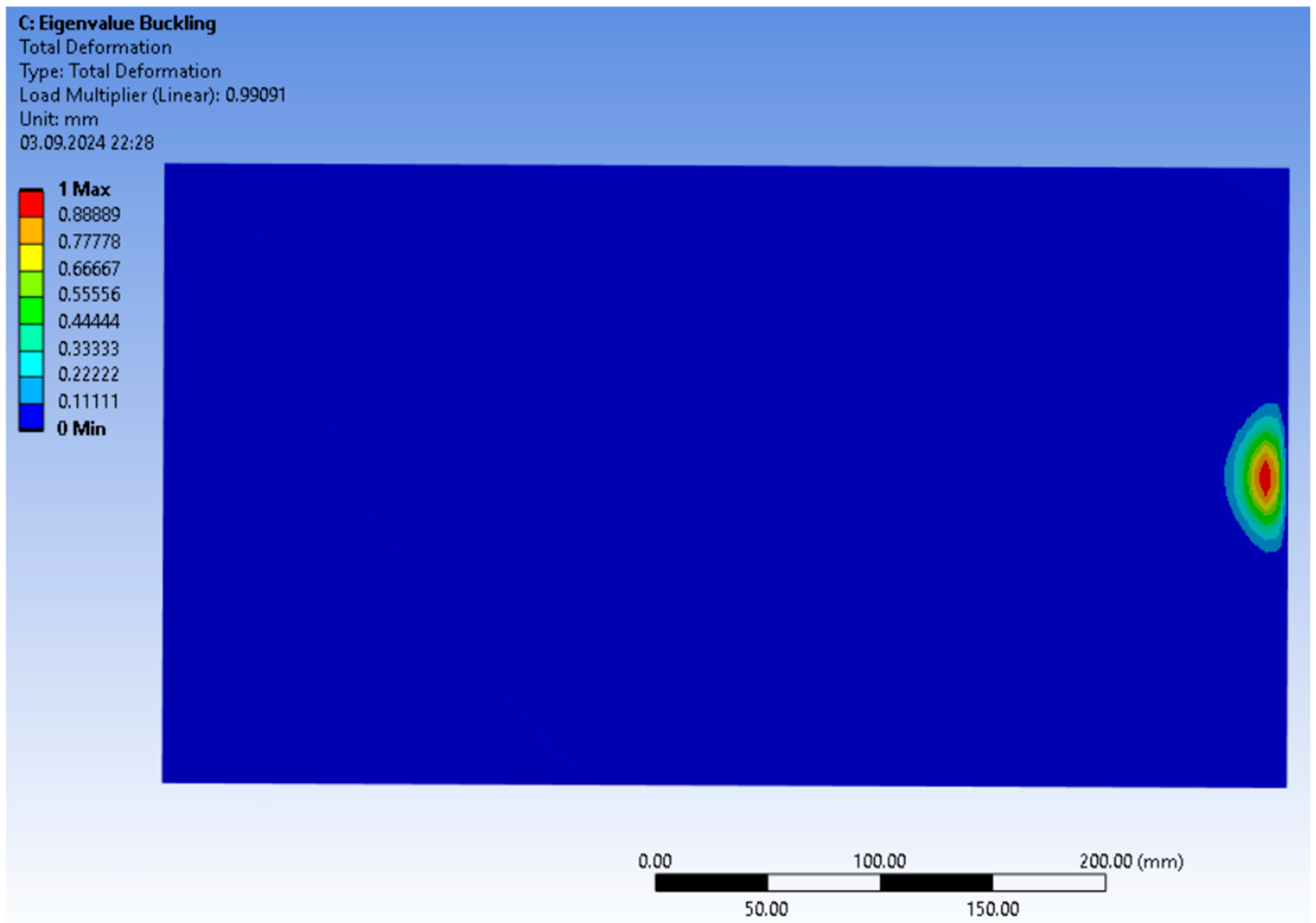
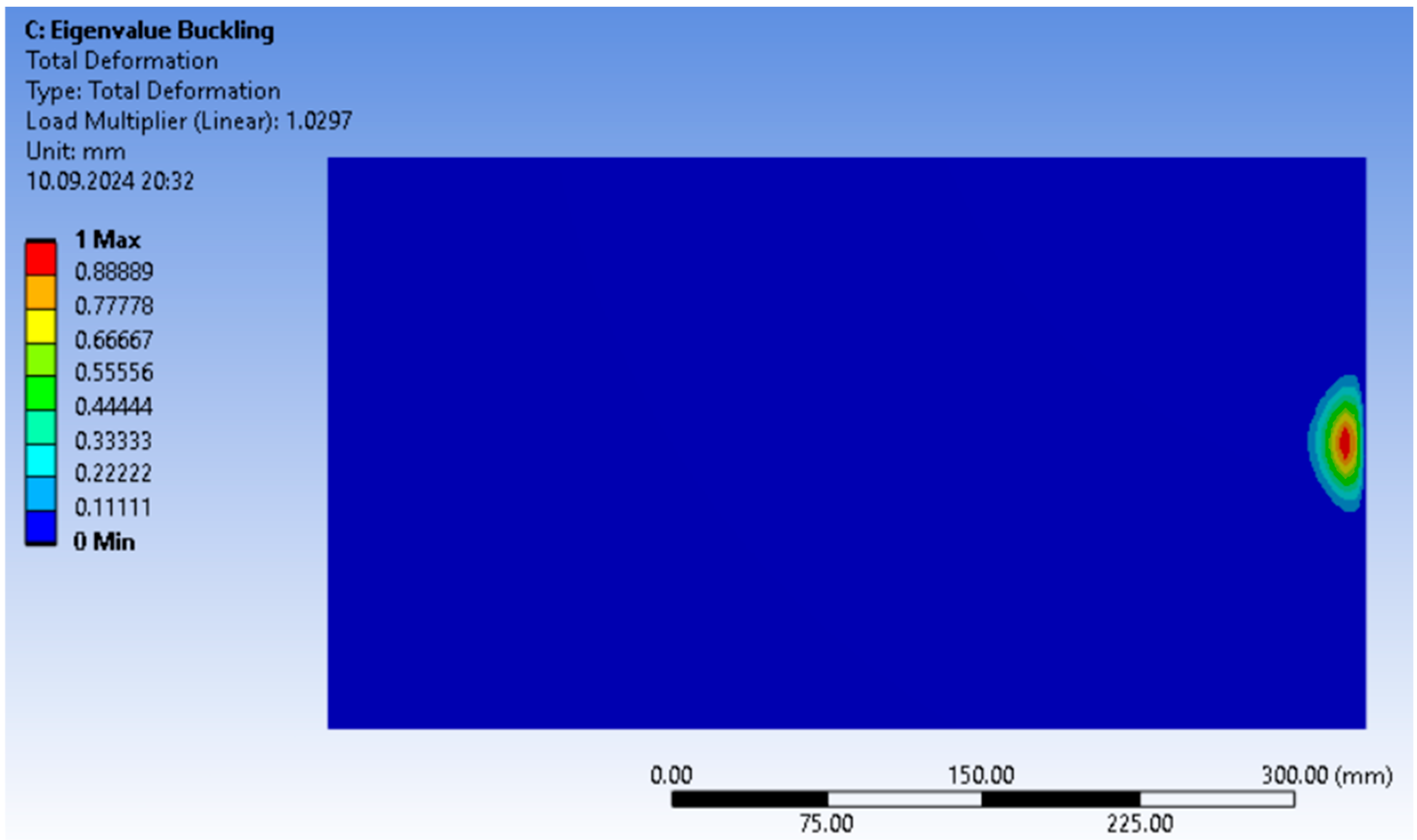
After the optimization via the genetic algorithm, the initial configuration before and after optimization was compared. The results are presented in Figure 12, Figure 13 and Figure 14.

Table 5. Comparison of pre- and post-optimization configurations.

After	Before
3	3	P1—Layer 1—number of surfaces
49.384	45	P2—Layer 1—Layer Orientation
3	3	P3—Layer 4—number of surfaces
32.219	45	P4—Layer 4—Layer Orientation
1	3	P5—Layer 3—number of surfaces
46.112	90	P6—Layer 3—Layer Orientation
3	3	P7—Layer 2—number of surfaces
71.937	90	P8—Layer 2—Layer Orientation
0.573	1.06	P10—Inverse Reserve Factor
1.029	0.99	P11—Total Deformation Load Multiplier

shows the collected values of the coefficients, where, despite a small difference in the value of the destruction factor, the stability factor for the configuration before optimization has significantly deteriorated. Structural parameters “before” were taken as an example from one of the most common sandwich-structure monocoque configurations used in Formula Student.

In Figure 13 and Figure 15, which show the Total Deformation Load Multiplier factor, a clear deformation area is visible on the right, where buckling occurs due to loading. This part has the highest deformation (red and yellow area), while the rest of the structure is practically unchanged (blue color). Buckling modes are natural deformation shapes for a given system of forces and structures. Different buckling modes can occur at different locations, and the first one (the lowest load multiplier) usually indicates the most probable buckling shape. Therefore, even if the pressure is uniform, the structure can naturally choose to buckle at a certain location.

10. Results and Discussion

Table 5 presents the structural parameters before and after optimization, along with the calculated coefficients. The Inverse Reserve Factor (IRF) decreased from 1.06 to 0.573. Since IRF is inversely proportional to the reserve factor against material failure, a lower value corresponds to a greater margin before reaching the ultimate strength limit [46]. In practical terms, the optimized design is less likely to fail under the prescribed loading conditions, thus offering improved safety and reliability.

Similarly, the Total Deformation Load Multiplier (TDLM) increased from 0.99 to 1.029. This coefficient represents the critical load factor at which global buckling or other instability phenomena occur [47]. An increase of ~3.9% means that the optimized sandwich monocoque can sustain a higher load before the onset of buckling. Although this numerical improvement may seem modest, even small gains in buckling resistance are valuable in high-performance automotive applications, where structural margins are often narrow and weight savings are critical.

The magnitude of improvements differs between IRF and TDLM because the optimization process primarily targeted ply orientations and layer configurations, variables that more strongly influence in-plane stiffness and failure resistance than global buckling. Hence, the IRF improvement is more pronounced, while TDLM improvements are incremental.

Candidate Configurations

Among the three candidate designs (Table 4), Candidate 3 exhibited the largest ply orientation angles, which enhanced its ability to redistribute stresses and delay material failure. This explains its favorable IRF value and improved resistance to localized strength limits. Candidate 2, by contrast, showed marginally better TDLM values, suggesting a configuration slightly more favorable to resisting global buckling. These results highlight the trade-off between local strength and global stability, which is a common feature in multi-objective composite optimization [48].

Limitations and Practical Implications

It should be emphasized that the current analysis was limited to loads acting perpendicular to the monocoque surface. In real service, vehicles are subjected to multi-directional loads, dynamic impacts, and manufacturing imperfections. The absence of robustness and uncertainty analysis represents a limitation of this study. Nevertheless, the results demonstrate that optimization via GA/MOGA can systematically refine ply orientation and layer thickness to enhance safety margins and structural performance without trial-and-error prototyping.

Future extensions should incorporate additional loading scenarios, stochastic variability in material properties, and benchmarking with alternative metaheuristics to validate robustness and broaden applicability.

11. Conclusions

• The optimization reduced the IRF from 1.06 to 0.573, indicating an increased reserve against material failure.
• The TDLM improved from 0.99 to 1.029, reflecting a modest but relevant gain in buckling resistance.
• Candidate 3 offered the most favorable balance, with improved failure resistance, while Candidate 2 slightly outperformed in stability. This demonstrates inherent trade-offs in multi-objective optimization.
• The improvements, though moderate, confirm that GA/MOGA within ANSYS can identify laminate configurations with enhanced safety margins, providing a structured pathway toward lightweight, high-performance sandwich monocoques.
• The study remains simulation-based; future work should include experimental validation, uncertainty quantification, and benchmarking against other optimization algorithms.