Single-Step Allowable Action Threshold Determination of Renewable Energy Automatic Generation Control Using Model-Based and Data-Driven Method

Abstract

Renewable energy automatic generation control (AGC) has the characteristics of rapid adjustment and flexibility, which play a critical role in frequency regulation. Abnormal outputs in renewable energy AGC may trigger frequency fluctuations and threaten grid security. To address the above problems in renewable energy, AGC, a combined model-based and data-driven method for determining the single-step allowable action threshold, is proposed. Firstly, an AGC model with multiple frequency-regulating units is built, and the threshold can be obtained through simulation considering system status parameters. Secondly, as the model-based method struggles to satisfy the requirement of rapidity, a data-driven model based on CNN-LSTM is employed to determine the threshold in real-time. The training data is provided by a model-based method. Considering the limited coverage and interpretability of neural networks, a statistical error-prevention method is proposed to avoid deviations. Then, an adaptive piecewise constant approximation algorithm is employezd to reduce threshold update frequency and the burden for dispatchers. Finally, an adaptive threshold adjustment method for extreme scenarios is proposed, ensuring the frequency regulation of renewable energy AGC under extreme scenarios. Through experiments, the reliability and validity of the proposed method in threshold determination and error prevention are validated.

1. Introduction

With the large-scale integration of renewable energy into the power system, the complexity of power grid operation has significantly increased [1,2,3]. The traditional frequency regulation mode, mainly composed of large thermal power and hydropower units, is facing severe challenges. Renewable energy output is highly volatile and changes rapidly. These characteristics increase both the amplitude and rate of system frequency deviations. At the same time, the frequency regulation capability of traditional generating units is gradually insufficient for the fast and flexible adjustments required by modern power systems. Thus, new requirements have been presented for the quantity and speed of frequency regulation resources.

In this context, renewable energy has become a key part of the active power balance and frequency regulation of the power grid. Automatic generation control (AGC) is essential for maintaining stable grid operation. Renewable energy AGC has become an important component of the overall AGC system and has attracted increasing attention in recent years [4,5,6]. In [7], the authors investigated a range of intelligent AGC strategies and their applications in renewable energy and distributed generation systems. Ziping Wu et al. [8] analyzed various AGC schemes applicable to wind-energy-based power plants. They also highlighted that low inertia and a weak primary response significantly affect AGC performance. Yiwei Qiu et al. [9] developed an SDE-based framework to model AGC signals as continuous random processes. This approach captures uncertainties arising from renewable generation and load variations. The method accurately captures both the probability distribution and temporal correlation of AGC signals. Lei Xi et al. [10] proposed a multi-agent distributed AGC strategy based on deep reinforcement learning to handle random disturbances caused by distributed renewable energy sources. By incorporating area control error and carbon emission levels into the reward function, the proposed method achieves optimal coordination among agents, effectively improving frequency regulation performance and reducing emissions. Yiqiao Xu et al. [11] proposed an online, adaptive optimization scheme for AGC that leverages BESSs to improve transient response. It introduces a modified Area Injection Error to quantify ramping needs and a distributed algorithm with adaptive learning rates to coordinate BESSs and conventional generators, effectively bridging the ramping capability gap.

The fast response of renewable energy AGC improves efficiency. However, it also introduces new safety and stability challenges [12]. Recently, the Iberian Peninsula blackout has prompted discussion about how to ensure the stability of electricity systems that have a high proportion of variable renewable energy. At the time of the incident, solar energy accounted for approximately 59% of Spain’s electricity supply, with wind providing around 12%, nuclear 11%, and gas 5% [13,14]. Currently, many error-prevention technologies are being widely researched for power grid safety. Fan Du et al. [15] proposed an error-proof adaptive optimization method for power dispatch that integrates real-time monitoring, state estimation, and fuzzy logic to improve calculation accuracy and operational efficiency. By controlling time redundancy, it ensures system stability, enables rapid generator start–stop and flexible load adjustment, and enhances the schedulability and economy of the power system. Taheri et al. [16] proposed a stochastic model that uses scenario sets generated by a Monte Carlo simulation algorithm to simulate the potential damage caused by events, selecting the optimal active grid operation to prevent erroneous actions, and thereby minimizing the impact of natural disasters on the power system. Zhukabayeva et al. [17] proposed a comprehensive framework to improve wireless sensor network security in smart grids. By combining traffic analysis, node classification, and machine learning, the method can effectively detect and prevent cyber threats, helping protect critical power infrastructure. Hussain et al. [18] developed a dual machine learning model to defend against IoT botnet attacks. It uses two ResNet-18 networks to detect early scanning behavior for prevention and to identify distributed denial-of-service attacks for timely mitigation. Laghari et al. [19] introduced a digital-signature-based security mechanism that ensures authentication, data integrity, and resilience against cyberattacks, including DoS, replay attacks, and FDIA. Zhang et al. [20] pointed out that most existing cybersecurity studies focus only on single-energy systems. To address this limitation, an optimal coordinated false-data injection attack and a deep-learning-based defense strategy were developed for multi-energy systems, and their effectiveness was demonstrated using integrated power–gas test systems.

The single-step allowable action threshold for renewable energy AGC refers to the maximum permissible change in output power for a renewable generating unit within one AGC step. This ensures that each regulation action remains within a safe range, preventing excessive power adjustments that could cause system frequency deviations or operational instability. It is clear that accurately determining the single-step allowable action threshold has become crucial for ensuring secure and stable grid operation [21,22,23]. The existing single-step allowable action threshold method for renewable energy AGC has obvious limitations, and cannot effectively adapt to the complex operational requirements of renewable energy grids. Specifically, it is difficult to make real-time and flexible adjustments based on the system’s operating status, with a risk of errors in operation. These deficiencies are reflected by the following four aspects:

(1)

The threshold tuning methods fail to adapt to the dynamic changes in system states, and lack real-time flexibility. Current methods can be divided into two categories. Model-based methods [24,25,26,27] rely on physical mechanisms and can compute thresholds accurately. However, they require multiple iterations and extensive simulations, making them too slow for AGC applications that require second-level responses. Consequently, they cannot keep up with rapid changes in system inertia or unit output in real-time. In contrast, data-driven methods can offer millisecond-level computational speed but are constrained by the coverage of their training datasets [28,29,30]. When the system operates beyond conventional training scenarios (such as during unexpected grid faults or unit start-up/shutdown events), the model may fail to adapt to the new system conditions, leading to error threshold outputs and risking the grid security.

(2)

The absence of effective error-prevention mechanisms leads to a high risk of error in operation. When abnormal operation occurs or training data contain noise, the threshold may deviate considerably from the true trend. Moreover, existing methods lack real-time identification and interception approaches for abnormal thresholds.

(3)

There is a little correlation between threshold update frequency and system state changes, leading to a lack of scheduling flexibility. In the current methods, thresholds are often updated every few minutes. This forces operators to monitor changes frequently, which lowers operational efficiency. In other cases, thresholds are updated at fixed intervals, failing to flexibly adjust the threshold based on the fluctuation characteristics of the system state.

(4)

The adaptability of thresholds under extreme scenarios is insufficient, leading to significant deviations. In extreme scenarios, if the threshold remains too tightly constrained, the rapid regulation capability of renewable energy is limited, making it difficult for it to play its role in the rapid stability process of the system.

In summary, existing methods struggle to adjust thresholds in real-time and carry a high risk of producing incorrect decisions. Therefore, it is imperative to develop a new threshold determination approach that can adapt to various typical operating scenarios. To address these problems, this paper proposes a method that integrates model-based and data-driven methods for determining the single-step allowable action threshold of renewable energy AGC. Firstly, a multi-unit AGC mechanism model is established. The model-based method then determines the single-step allowable action threshold for renewable energy AGC through iterative simulations. Then, the model-based method provides training samples for the data-driven method. However, since the accuracy of the neural network output strongly depends on the coverage and diversity of the training dataset, large deviations or even misjudgments may occur when the data distribution changes or the system contains abnormal information. An adaptive piecewise threshold optimization method is introduced to balance the threshold update frequency with dispatching flexibility. This reduces unnecessary updates and lowers the burden on operators. Finally, an adaptive adjustments method is introduced for extreme conditions (such as extreme weather events or grid fault recovery events) to ensure that renewable energy can still provide rapid and effective regulation under these critical circumstances. The main contributions of this paper can be summarized as follows:

(1)

A “data-driven dominated, model-based assisted” approach is proposed for determining the single-step allowable action threshold for renewable energy AGC. In this framework, a multi-unit AGC mechanism model is first constructed to characterize the dynamic response behaviors among multiple frequency-regulating units. The model-based approach is then utilized to generate a large number of simulation samples under diverse operating conditions, which serve as the foundational training data for the data-driven method. Using a CNN-LSTM neural network employed in the data-driven method, the proposed method is capable of determining a single-step allowable action threshold that adapts in real-time to the system operating conditions.

(2)

To address potential deviations and misjudgments in neural network outputs caused by limited training coverage or abnormal data, an error-prevention and verification mechanism is designed. This mechanism continuously monitors model outputs, and intercepts abnormal threshold decisions before they propagate to AGC execution. As a result, the operational safety and reliability of the control system are enhanced.

Moreover, for extreme weather events (such as typhoons, sandstorms, or cold waves) or grid fault recovery scenarios, an adaptive adjustment strategy is introduced. This strategy dynamically extends the threshold boundary, ensuring that renewable energy resources can still perform fast, flexible, and effective regulation under extreme or uncertain conditions.

(3)

An adaptive piecewise threshold optimization method based on system state fluctuation features is further developed. This method adjusts the frequency of threshold updates according to the fluctuation characteristics of the system state. It balances threshold update frequency and dispatching flexibility. Consequently, the proposed approach not only reduces the computational and operational burden of system operators but also improves the real-time performance and robustness of renewable energy AGC systems.

The rest of the paper is organized as follows. Section 2 introduces the overall framework. Section 3 illustrates the specific methods for determining the single-step allowable action threshold for renewable energy AGC. Section 4 presents the experimental setting, results, and discussion, and Section 5 concludes this paper.

2. The Introduction of Overall Framework

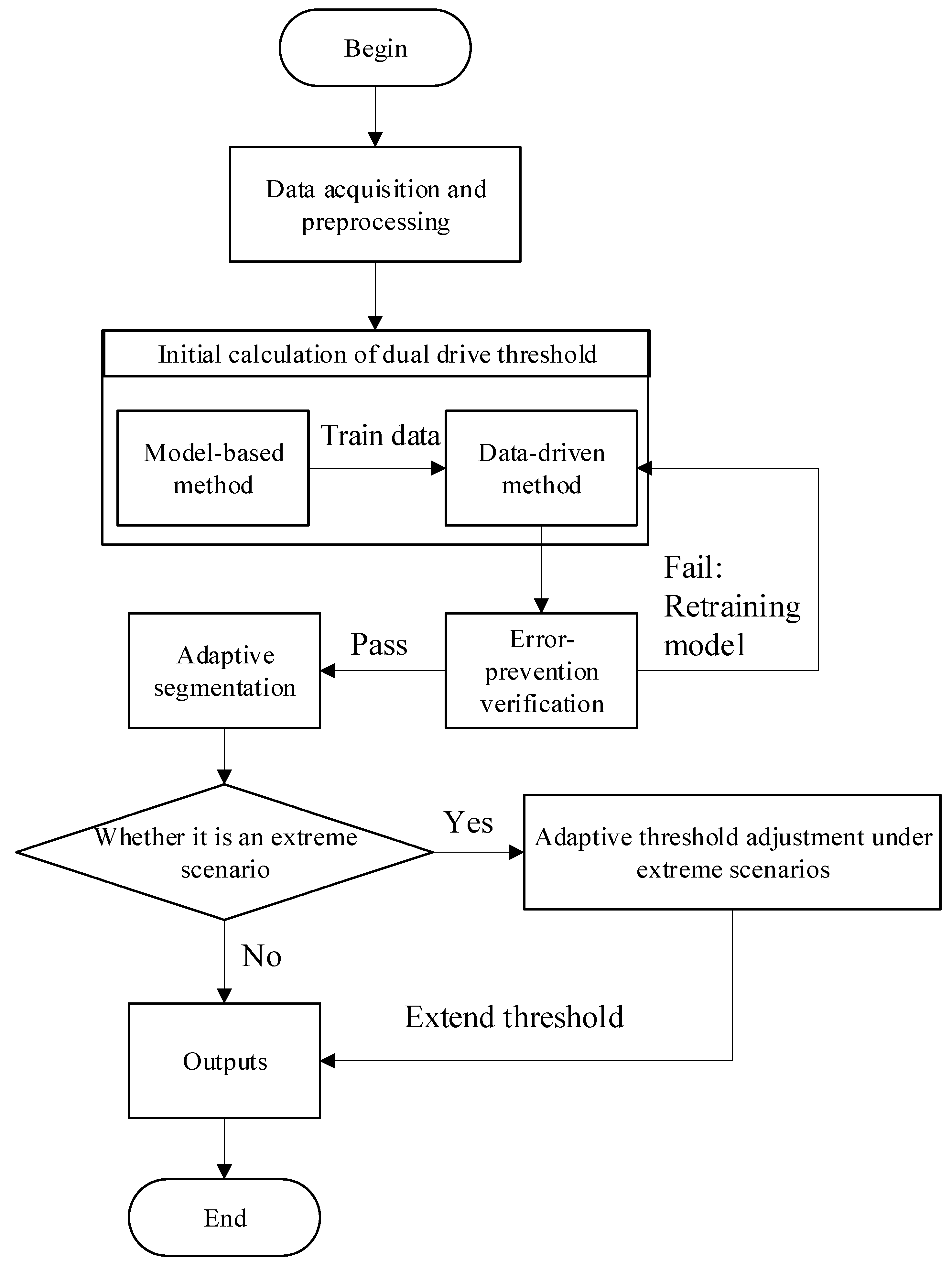
The overall framework of this method is as shown in Figure 1. First, system operation data are collected and preprocessed. Then, the single-step allowable action threshold for renewable energy AGC is determined through a hybrid model-based and data-driven method. The model-driven method iteratively obtains thresholds via AGC simulation and provides training samples for the subsequent data-driven learning. The data-driven method employs a CNN-LSTM network to determine threshold. Considering potential risk deviations caused by the uncertainty of data-driven, an error-prevention validation mechanism is introduced. If the threshold exceeds the safety limit, the output is blocked, and half of the safety threshold is directly adopted and retrains model. For the thresholds that pass the validation, an adaptive piecewise constant approximation (APCA) algorithm is applied to optimize segmentation, reducing updating frequency and lowering dispatching workload. Finally, the operating scenario is identified. Under normal conditions, the threshold is used directly. Under extreme conditions, it is expanded to allow renewable units to fully utilize their fast regulation capability. The proposed method is designed for provincial-level AGC master stations (dispatch centers). It is applied on the dispatch side, where AGC commands are generated. In engineering practice, the method only requires several key parameters of each generating unit—such as rated capacity, governor parameters, inertia constants, and droop coefficients—to run the AGC simulation model. These parameters are normally reported to the dispatch center when a unit is commissioned, as part of the standard grid-connection data submission.

Through the above framework, the single-step allowable action threshold for renewable energy AGC can be determined effectively and quickly. The details of each part are described in the following chapters.

3. Materials and Methods

3.1. Single-Step Allowable Action Threshold Determination of Renewable Energy AGC Using Model-Based Method

The single-step allowable action threshold of renewable energy AGC defines the maximum output adjustment for a renewable unit, such as wind or photovoltaic generation. It ensures that each control step remains within a safe range, preventing any impact on system security or operational stability. This section first establishes the multi-unit automatic generation control model. Then, the model is employed in simulations to determine the single-step allowable action threshold for renewable energy AGC.

3.1.1. The AGC Model of Renewable Energy

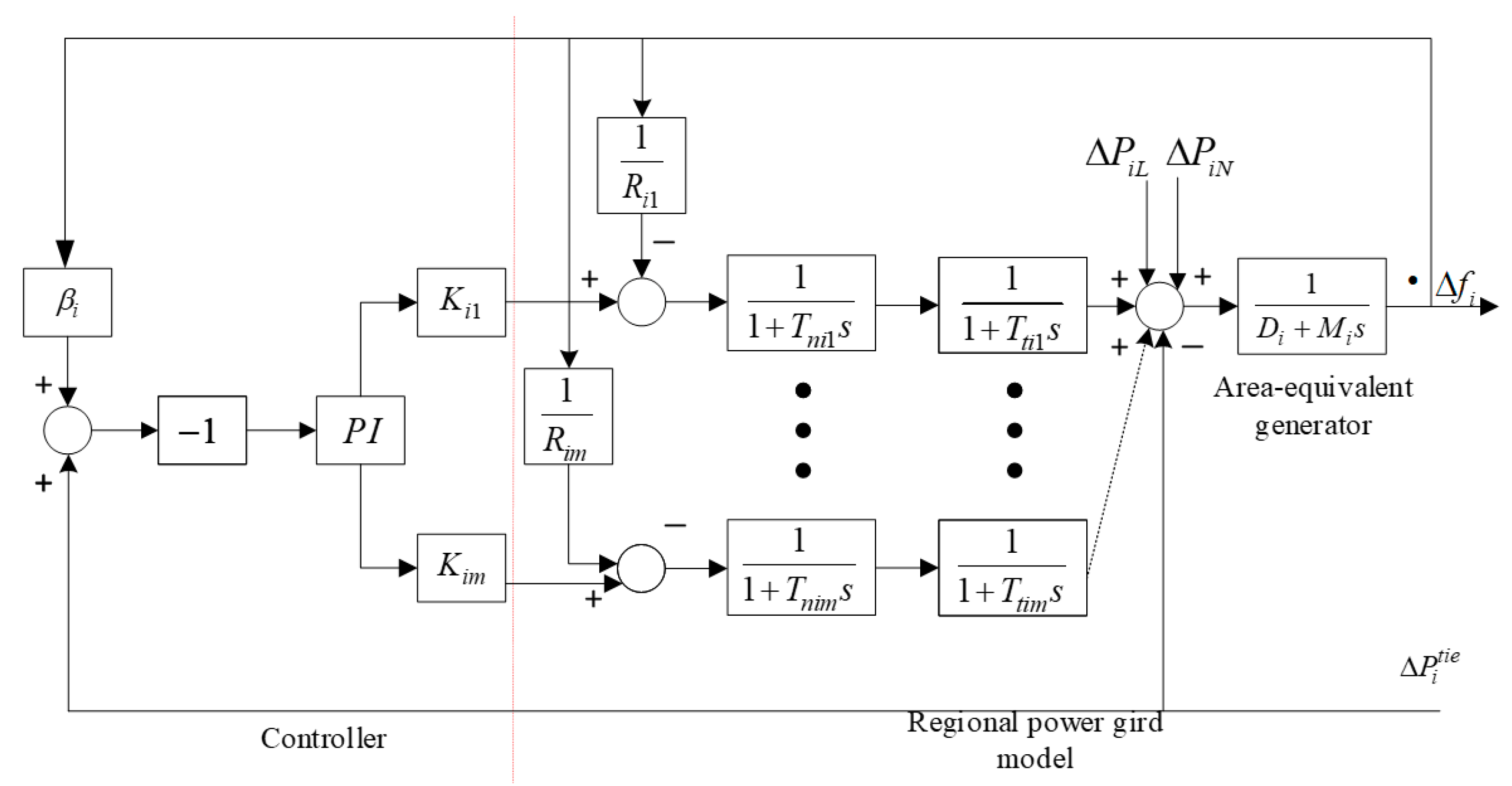
This section establishes an AGC model that includes multiple frequency-regulating units, which will be used in subsequent simulations to determine the single-step allowable action threshold. As shown in Figure 2 and

Table 1. The parameters of the automatic generation control model.

Title 1	Title 2
i	The i-th area
$\Delta P_{iL}$	Total load deviation of area i
$\Delta P_{iN}$	Single-step renewable energy AGC command deviation of area i
$\Delta f_i$	Simulated frequency deviation of area i
${\beta }_i$	Frequency deviation coefficient of area i
PI	Proportional–Integral (PI) controller
$K_{i1}~K_{im}$	Allocation coefficients of the PI controller for units 1 to m in area i
${\displaystyle \frac{1}{R_{i1}}}~{\displaystyle \frac{1}{R_{im}}}$	Primary frequency regulation models of units 1 to m in area i
$M_i$	Total inertia of area i
$\Delta f_{imax}$	Maximum allowable frequency deviation of area i
$\Delta P_i^{tie}$	Tie-line power exchange deviation
$D_i$	Load damping coefficient of area i
${\displaystyle \frac{1}{1+T_{ni1}s}}$, ${\displaystyle \frac{1}{1+T_{ti1}s}}$	Model of the first generating unit in area i
${\displaystyle \frac{1}{1+T_{nim}s}}$, ${\displaystyle \frac{1}{1+T_{tim}s}}$	Model of the m-th generating unit in area i
${\displaystyle \frac{1}{D_i+M_{i}s}}$	Generator model of area i

, the AGC model consists of a load frequency controller and a regional power grid model [31,32]. A Proportional–Integral (PI) control algorithm is employed for the load frequency controller, while the regional grid model mainly comprises frequency-regulating unit models, including the generator, prime mover, and governor. In this model, the entire generation area is represented by an area-equivalent generator. We regard the generation output of renewable energy as a part of load disturbance ($\Delta P_{iN}$), rather than directly participating in frequency regulation. The controller calculates the total active power regulation command based on the Area Control Error (ACE). This total command is then distributed among all frequency-regulating units according to their respective distribution coefficient, obtaining the individual active power adjustment signal for each unit. Through this process, the AGC can achieve coordinated active power regulation and maintain system frequency stability.

The following sections provide detailed descriptions of the generator, turbine, and governor models.

(a)

Generator Model

In the generator model, each generator unit can be represented as a turbine driving a generator [33]. According to the principle of inertia, when the output power changes, the mechanical part will exist mechanical inertia, and its changes to lag behind that of the electromagnetic power. As a result, a power deviation occurs. Equation (1) describes the relationship between the power deviation and the torque deviation.

$$\Delta P_m-\Delta P_e={\omega }_0(\Delta T_m-\Delta T_e)+(T_{m0}-T_{e0})\Delta {\omega }_r,$$

(1)

where $\Delta {\omega }_r$ denotes generator angular velocity deviation, ${\omega }_0$ denotes rated angular velocity of generator, $\Delta T_e$ denotes electromagnetic torque deviation, $\Delta T_m$ denotes mechanical torque deviation, $\Delta P_m$ denotes mechanical power deviation, and $\Delta P_{\mathrm{e}}$ denotes electromagnetic power deviation. In the quasi-steady state, the electromagnetic torque is equal to the mechanical torque, so Equation (1) can be simplified as Equation (2).

$$\Delta P_m-\Delta P_e={\omega }_0(\Delta T_m-\Delta T_e).$$

(2)

Define the moment of inertia as $I$; then, the relationship between rotational speed and torque can be expressed as Equation (3).

$$I{\displaystyle \frac{d(\Delta \omega )}{dt}}=\Delta T_m-\Delta T_e.$$

(3)

Set the inertia time constant of the generator as $T={\omega }_{0}I$. Equation (2) can be transformed as follows:

$$\Delta P_m(s)-\Delta P_e(s)=Ts\Delta \omega (s).$$

(4)

When no active power disturbance occurs, mechanical and electromagnetic power remain balanced. Thus, the system frequency remains stable without deviation. When no active power disturbance occurs in the system, the mechanical power and electromagnetic power of the generator remain balanced, and the system frequency remains stable, without deviation. However, when an active power disturbance occurs, a transient imbalance arises between the mechanical and electromagnetic powers, leading to frequency fluctuation in the system. In this study, the active power disturbance is defined as the change in active load, which consists of two components: (1) a component independent of frequency changes $\Delta P_D$; (2) a component dependent on frequency changes $\Delta P_D=D\Delta {\omega }_r$. According to the law of energy conservation, the deviation of the electromagnetic power is equal to the deviation of the active load power, as shown in Equation (5).

$$\Delta P_e=\Delta P_L+D\Delta {\omega }_r,$$

(5)

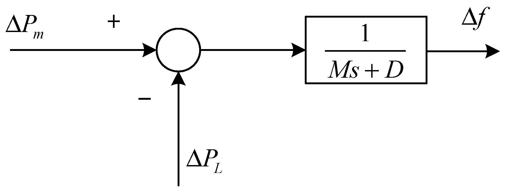
where D represents the damping coefficient of the load. From Equations (4) and (5), the equivalent generator model of the area can be obtained, as shown in Figure 3.

(b)

Turbine and Governor Model

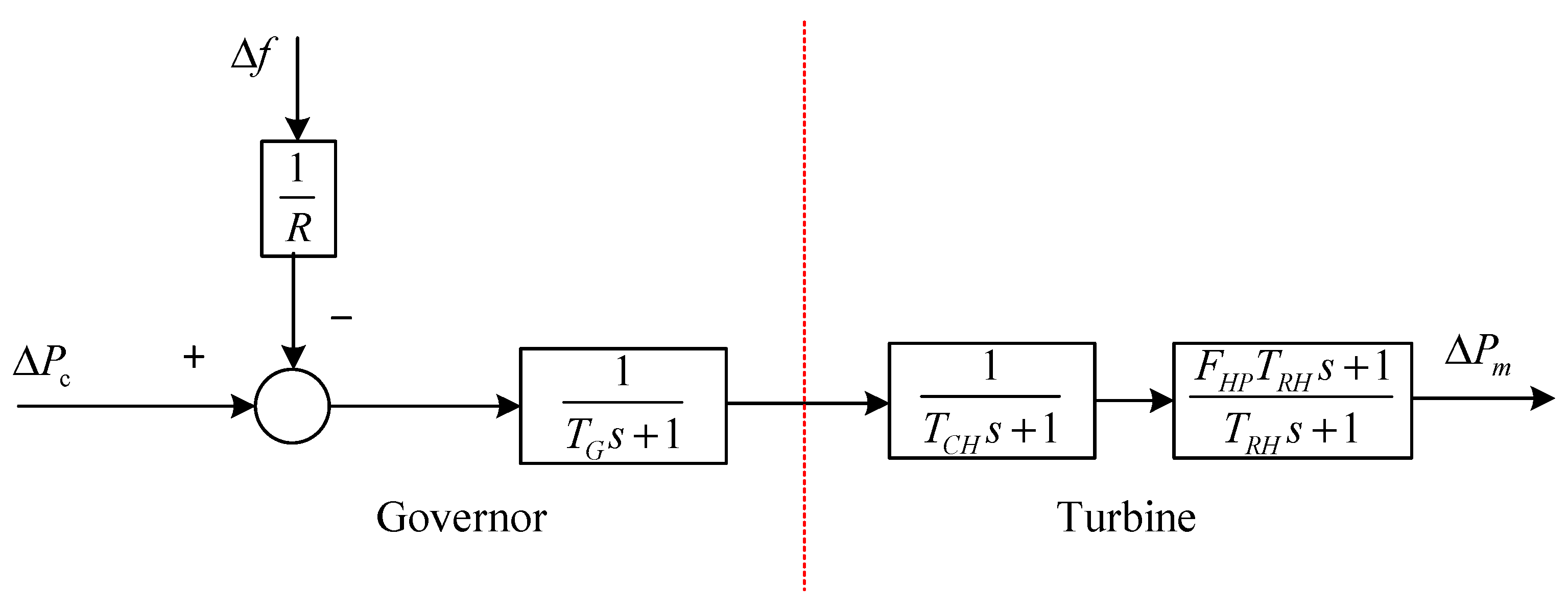
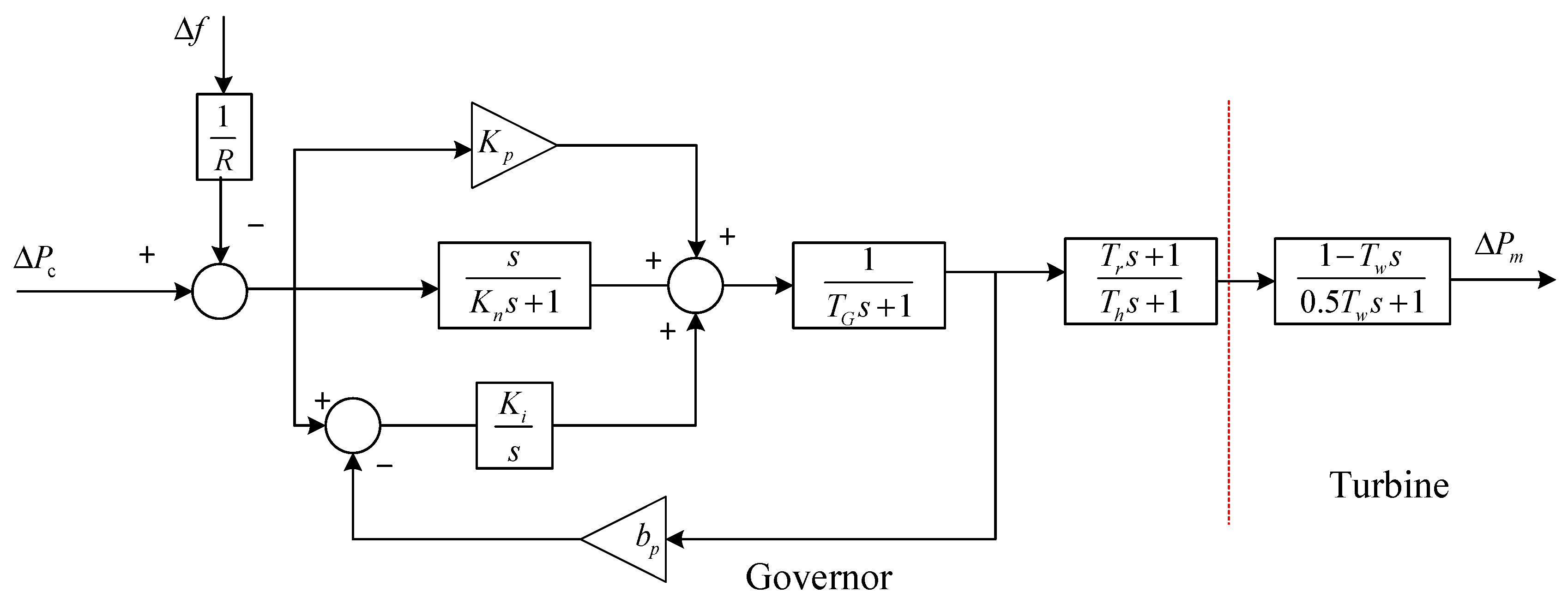
In this paper, the turbine includes both hydraulic and steam types, corresponding to hydro and thermal generating units. The steam turbine can be categorized into non-reheat and reheat types [34]. The following sections briefly introduce the models of non-reheat steam turbines, reheat steam turbines, and hydraulic turbines, along with the corresponding governor models for each type of turbines.

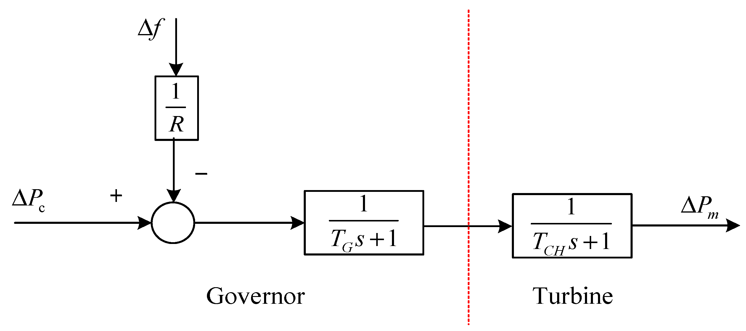
The turbine and governor model of the non-reheat steam turbine is shown in Figure 4.

In Figure 4, $T_G$ denotes the time constant of governor, $T_{CH}$ denotes the non-reheat time constant, and R denotes the droop coefficient of governor, numerically defined as the ratio of angular frequency to valve opening degree.

The turbine and governor model of the reheat steam turbine is shown in Figure 5. Compared with the non-reheat steam turbine, it includes an additional stage of secondary power generation.

For Figure 6, $T_w$ is the water starting time constant, representing the time required for the hydraulic head to accelerate the water flow in the gate from rest to a certain velocity. Compared with the steam turbine governor, the governor of hydraulic turbine includes a transient compensation part. $T_h$ is the transient droop time constant of the hydraulic turbine governor, and $T_r$ is the reset time constant of the governor. In addition, a PID module is employed in the governor of the hydraulic turbine to enable a fast response to frequency changes. In practical applications, pure derivative control belongs to advanced control and is difficult to implement. Thus, it is typically replaced by the term $s$/$(K_{n}s+1)$, where $K_n$ serves as the proportional coefficient. Moreover, hydro units have a permanent droop coefficient $b_p$, which affects the depth of their participation in primary frequency regulation [35].

3.1.2. The Influencing Factors of Single-Step Allowable Action Threshold for Renewable Energy AGC

It is worth noting that the single-step allowable action threshold is not a fixed constant. It can change with the operating conditions of the power system. For example, when multiple thermal generating units are connected in the grid, the inertia of the system increases and the disturbance-resisting capability of the grid improves, causing the single-step allowable action threshold to rise accordingly. Therefore, this section firstly introduces the factors influencing the single-step allowable action threshold and the methods for determining each factor. Then, we explain how to determine the threshold based on these various factors.

(a)

The Inertia of Power Grid

In the power system, the inertia is analogous to the resistance of rotating equipment (such as generator rotors) to changes in rotational speed. This resistance is derived from the kinetic energy stored in the rotating masses, quantified as the moment of inertia. The inertia serves as a key indicator, and its influence manifests as the system characteristics [36,37,38].

Without considering the virtual inertia for renewable energy-generating units, the moment of inertia is mainly caused by synchronous generators, such as the steam generator and hydraulic generator, and can be converted into energy. The kinetic energy stored in the rotor during rotation is shown in Equation (6):

$$E_k={\displaystyle \frac{1}{2}}J{\omega }^2,$$

(6)

where $E_k$ and J are the kinetic energy of a synchronous generator and its moment of inertia. $\omega$ represents the mechanical angular velocity of the rotor.

When the system is disturbed, the synchronous generator rotor releases or stores energy by increasing or decreasing its stored kinetic energy to compensate for the power imbalance. This process can maintain system stability and prevent excessive frequency fluctuations. Neglecting the small angular velocity differences among generator rotors, the stored energy can be expressed by Equations (7) and (8):

$$\Delta E_i={\displaystyle \frac{1}{2}}{J}_i({\omega }_m^2-{\omega }_n^2);$$

(7)

$$\Delta E=\Delta E_1+\Delta E_2+\cdots +\Delta E_n={\displaystyle \sum _{i=1}^n\Delta E_i},$$

(8)

where $J_i$ and $\Delta E_i$ are the moment of inertia for the i-th synchronous generator and the energy released or stored by its rotor. ${\omega }_n$ and ${\omega }_m$ are the angular velocity of the synchronous generator before and after the disturbance. $\Delta E$ denotes the total energy released or stored by all synchronous generators. By combining Equations (7) and (8), we can obtain

$$\Delta E={\displaystyle \frac{1}{2}}({\omega }_m^2-{\omega }_n^2){\displaystyle \sum _{i=1}^n{J}_i}.$$

(9)

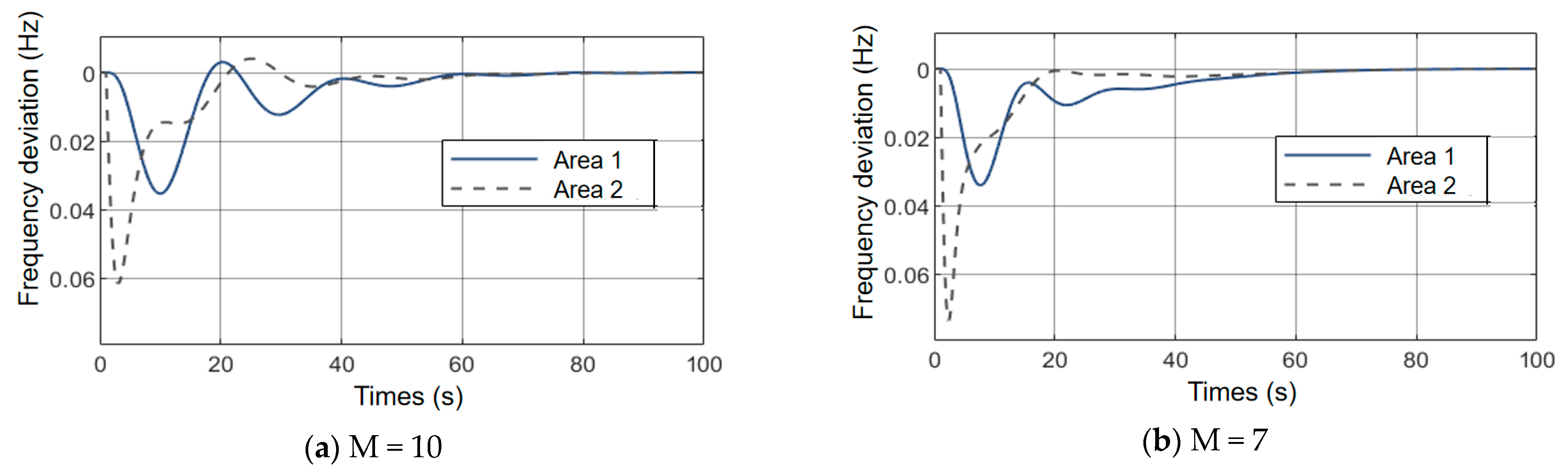
In Equation (9), it is obvious that a system with larger inertia experiences smaller frequency fluctuations, allowing a wider AGC single-step adjustment range. Figure 7 shows the simulation results of AGC with different inertia levels under the same disturbance conditions, where M represents the inertia of the systems. Therefore, the inertia of system is one of the key factors influencing the single-step allowable action threshold.

(b)

Frequency Bias Coefficient of Power System

When the active power generation and load demand in a power system are unbalanced, the primary frequency regulation in each area can adjust its generation output ($\beta \Delta f$) based on its natural frequency characteristic coefficient ($\beta$). Meanwhile, power is transmitted through tie-lines between areas to support the region experiencing the disturbance and help reestablish the power balance between generation and load. Set the frequency deviation after primary frequency regulation as $\Delta f$, and the total load disturbance of the system as $\Delta P$. Then, the natural frequency characteristic coefficient of the system can be expressed as follows:

$$\beta =-{\displaystyle \frac{\Delta P}{\Delta f}}.$$

(10)

To restore frequency and tie-line power to their scheduled values, the system must adjust generator outputs through secondary frequency control. The area control error (ACE) serves as the primary control signal guiding the AGC active power outputs in the control area [39]. In actual engineering applications, the natural frequency characteristic coefficient $\beta$ is difficult to determine. Therefore, the frequency bias coefficient ($B$) is employed to compute ACE. In TBC mode, it is necessary to adjust the power outputs of each control area to match its power supply responsibility, and ACE typically is based on the frequency deviation $\Delta f$ and tie-line power exchange deviation $\Delta P_{tie}$, defined as

$$ACE=\Delta P_{tie}+B\Delta f.$$

(11)

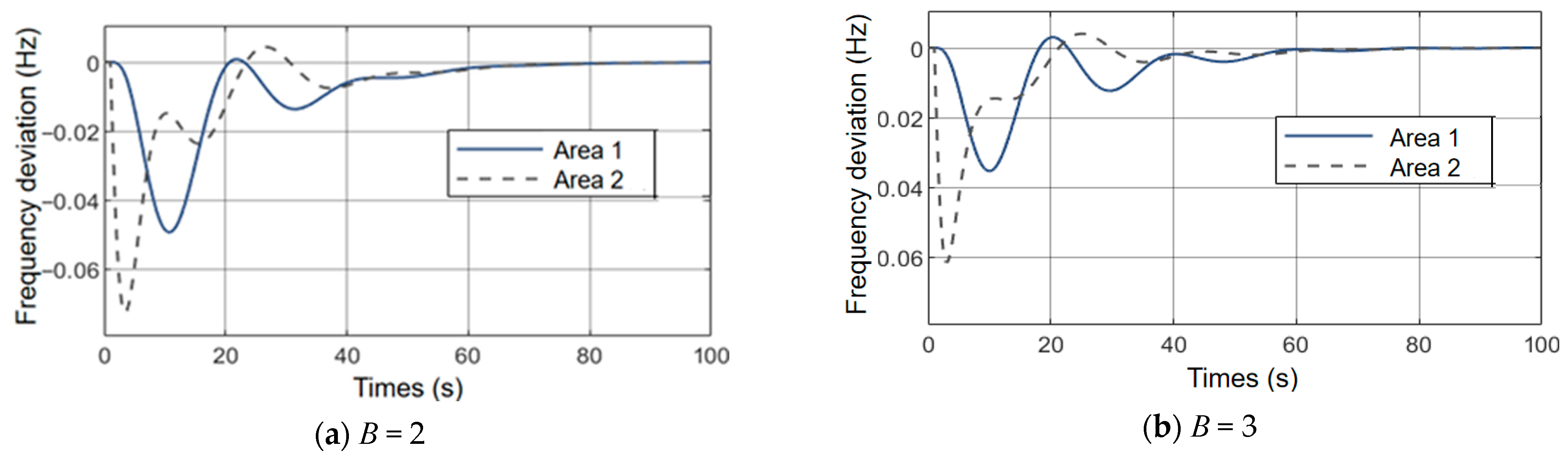
It is clear that $B$ reflects the steady-state frequency deviation caused by power disturbances, representing the system’s sensitivity to power fluctuations. A larger value of $B$ indicates better frequency stability and a higher single-step action threshold for renewable energy AGC. Figure 8 shows the simulation results for different values of $B$. Under the same disturbance, systems with larger $B$ exhibit smaller frequency fluctuations, demonstrating that the frequency bias coefficient is an important factor influencing the action threshold.

It is assumed that the frequency bias coefficient $B$ consists of the frequency bias coefficient of load $B_L$ and generator $B_G$, as follows:

$$B=B_L+B_G.$$

(12)

Due to the fact that system loads are typically composed of static and dynamic loads, $B_L$ can be represented as

$$B_L={\displaystyle \frac{K_L^{*}{K}_1{P}_L}{100f_N}}+K_M(1-K_1)P_L,$$

(13)

where $P_L$ denotes the total load of the systems, $K_1$ denotes the proportion of static load, $K_L^{*}$ and $K_M$ are the frequency regulation coefficient of the load and frequency regulation weight coefficient of dynamic load, and $f_N$ denotes the rated frequency of the systems. In this model, there are steam turbine generating units and hydro-turbine generating units participating in frequency regulation. Ignoring the dead zone of the governor, the frequency deviation coefficient of the generator $B_G$ can be obtained as

$$B_G={\displaystyle \sum _{i=1}^n{B}_{Gi}},$$

(14)

where $B_{Gi}$ denotes the contribution of the i-th unit to the $B$ coefficient. It is evident that $B$ is a nonlinear and time-varying parameter, which is affected by factors including load fluctuations and the output of thermal and hydro-units.

(c)

Maximum Allowable Frequency Deviation

The secure operation of the power grid depends on the system frequency being maintained within an acceptable range. Frequency deviations, involving either an excessive rise or drop, can cause the loss of synchronism in the generator, device failure, and even large-scale blackouts. Therefore, defining an appropriate maximum allowable frequency deviation is essential to ensure the security and reliability of systems.

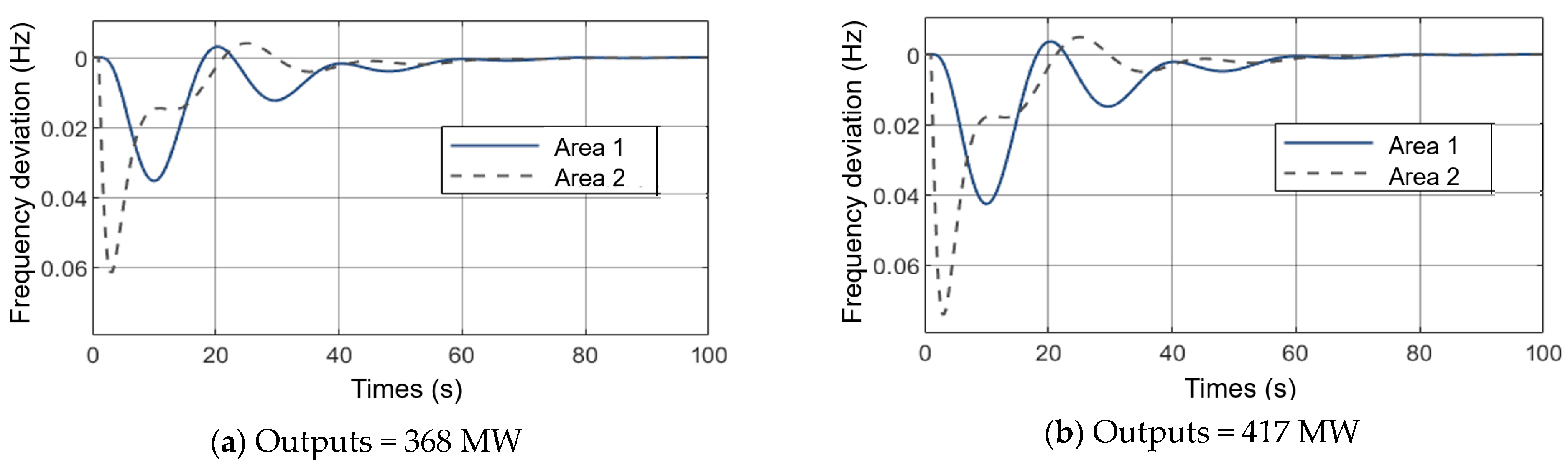
Since the adjustment of generator output directly affects the active power balance and subsequently the frequency of systems, it can be regarded as a disturbance. A larger unit output will result in larger frequency fluctuations in the system, as shown in Figure 9. Thus, a higher maximum allowable frequency deviation can correspond to a larger single-step allowable action threshold. The maximum allowable frequency deviation is an important factor in the single-step allowable action threshold.

Under a high proportion of renewable energy, due to the large fluctuations in wind and photovoltaic outputs and limited frequency regulation capabilities, the system frequency is more prone to changes. As a result, the frequency-regulating units must adjust their output to maintain a stable frequency, leading to increased fuel consumption and operational costs. Therefore, from the perspective of frequency regulation economy, it is reasonable to appropriately relax the frequency limits when the outputs of renewable energy are high, as shown in Equation (15):

$$f=k{P}_R+b,$$

(15)

where $f$ denotes the maximum allowable frequency deviation, $k$ and $d$ are the proportional coefficient and bias, and $P_R$ denotes the total outputs of renewable energy units.

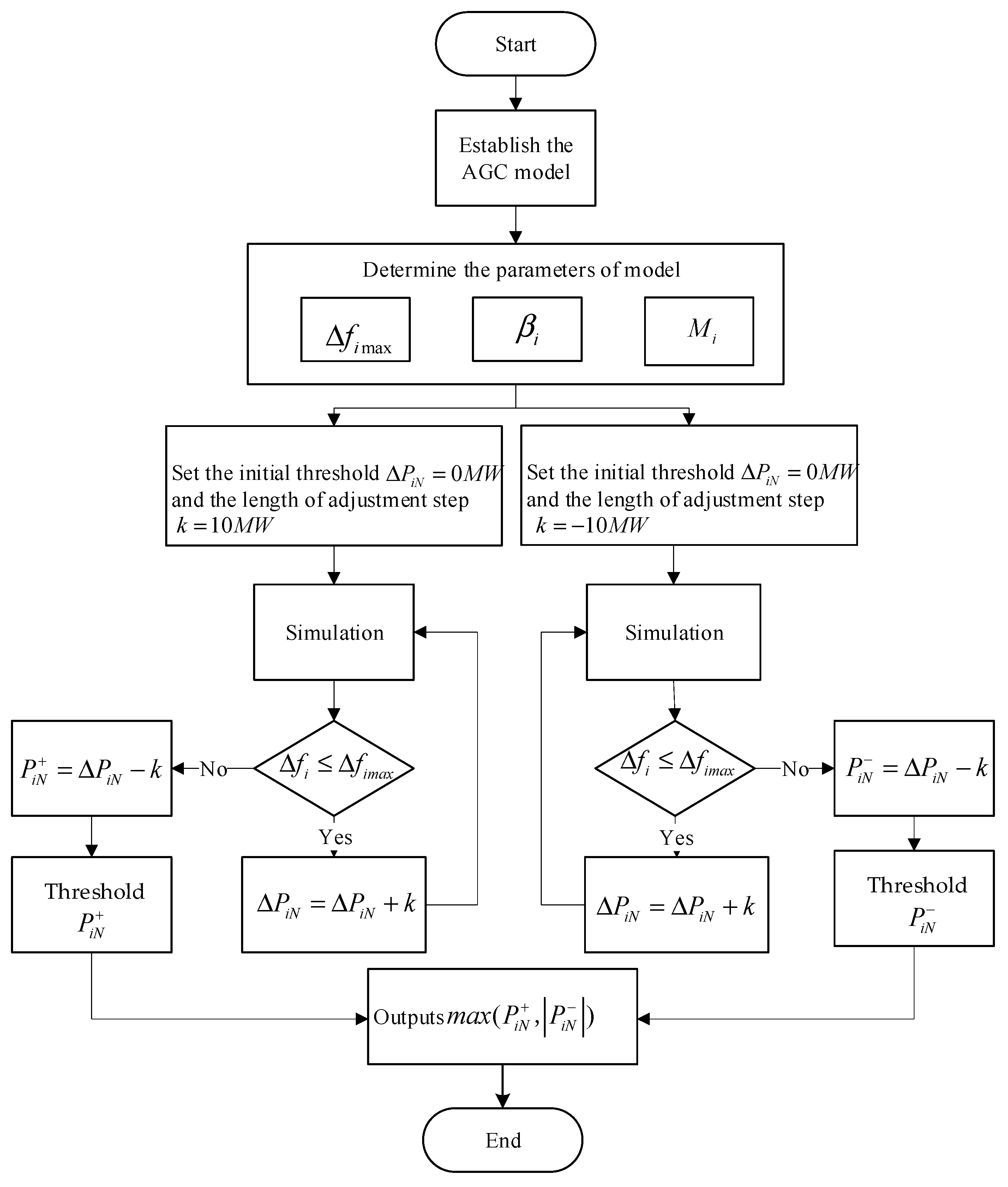
3.1.3. The Determination of a Single-Step Allowable Action Threshold Using Model-Based Method

The specific determination method is illustrated in Figure 10. Firstly, the PI controller coefficients $K_{i1}~K_{im}$, the primary frequency control models of each regulating unit, and the total load deviation $\Delta P_{iL}$ of area i are calculated. These parameters usually remain unchanged during the simulation process. According to the current system state, the frequency deviation coefficient $B$, total system inertia $M_i$, and maximum allowable frequency deviation $\Delta f_{imax}$ can be determined. Then, the initial threshold $\Delta P_{iN}=0 \mathrm{M}\mathrm{W}$ and the length of adjustment step $k$ are initialized. Through simulations, the frequency deviation $\Delta f_i$ is obtained and compared with the maximum allowable frequency deviation $\Delta f_{imax}$. If $\Delta f_i$ ≤ $\Delta f_{imax}$, $\Delta P_{iN}$ is increased by one length of adjustment step $k$. This process is repeated until $\Delta f_i>\Delta f_{imax}$, and the corresponding value of $P_{iN}^{+}=\Delta P_{iN}-k$ or $P_{iN}^{-}=\Delta P_{iN}-k$ are obtained as the positive or negative single-step allowable action threshold. Finally, the absolute values of the two thresholds are compared, and the larger one is selected as the single-step allowable action threshold of renewable energy AGC.

The data obtained by the model-based method are used to augment the existing dataset and are combined as the input for the data-driven model in Section 3.

3.2. Single-Step Allowable Action Threshold for the Determination of Renewable Energy AGC Using Data-Driven Method

The determination of the single-step allowable action threshold for renewable energy AGC essentially involves establishing the mapping relationship between some variables (such as unit output and inertia) and the threshold. However, due to the nonlinear characteristic of these variables, the existence of one-to-many mapping relationships, simple linear regression, or polynomial fitting methods struggle to accurately determine the threshold. It is necessary to employ neural networks to extract the underlying patterns and construct the corresponding mapping relationships. In this paper, a Convolutional Neural Network–Long Short-Term Memory (CNN-LSTM) model is proposed. The CNN-LSTM combines the powerful feature extraction capability of the Convolutional Neural Network (CNN) and the temporal dependency learning ability of the Long Short-Term Memory (LSTM). It is employed to model the relationship between unit output, system inertia, system load, and the renewable energy AGC single-step allowable action threshold, enabling the determination of the corresponding action threshold.

3.2.1. Normalization Processing

The time-series parameters, including the single-step allowable action threshold, system inertia, output, and system load, differ in scale and measurement units. Therefore, it is essential to normalize the experimental data before training the LSTM network to prevent the model from being overly sensitive to variations. The min–max normalization algorithm, as shown in Equation (16), is applied to preprocess the data.

$$y_i^j={\displaystyle \frac{x_i^j-\min (x^j)}{\max (x^j)-\min (x^j)}},$$

(16)

where $x_i^j$ denotes the i-th time series data of j-th category. $\max (x^j)$ and $\min (x^j)$ are the maximum and minimum values of the j-th category data, respectively.

3.2.2. CNN-LSTM Model

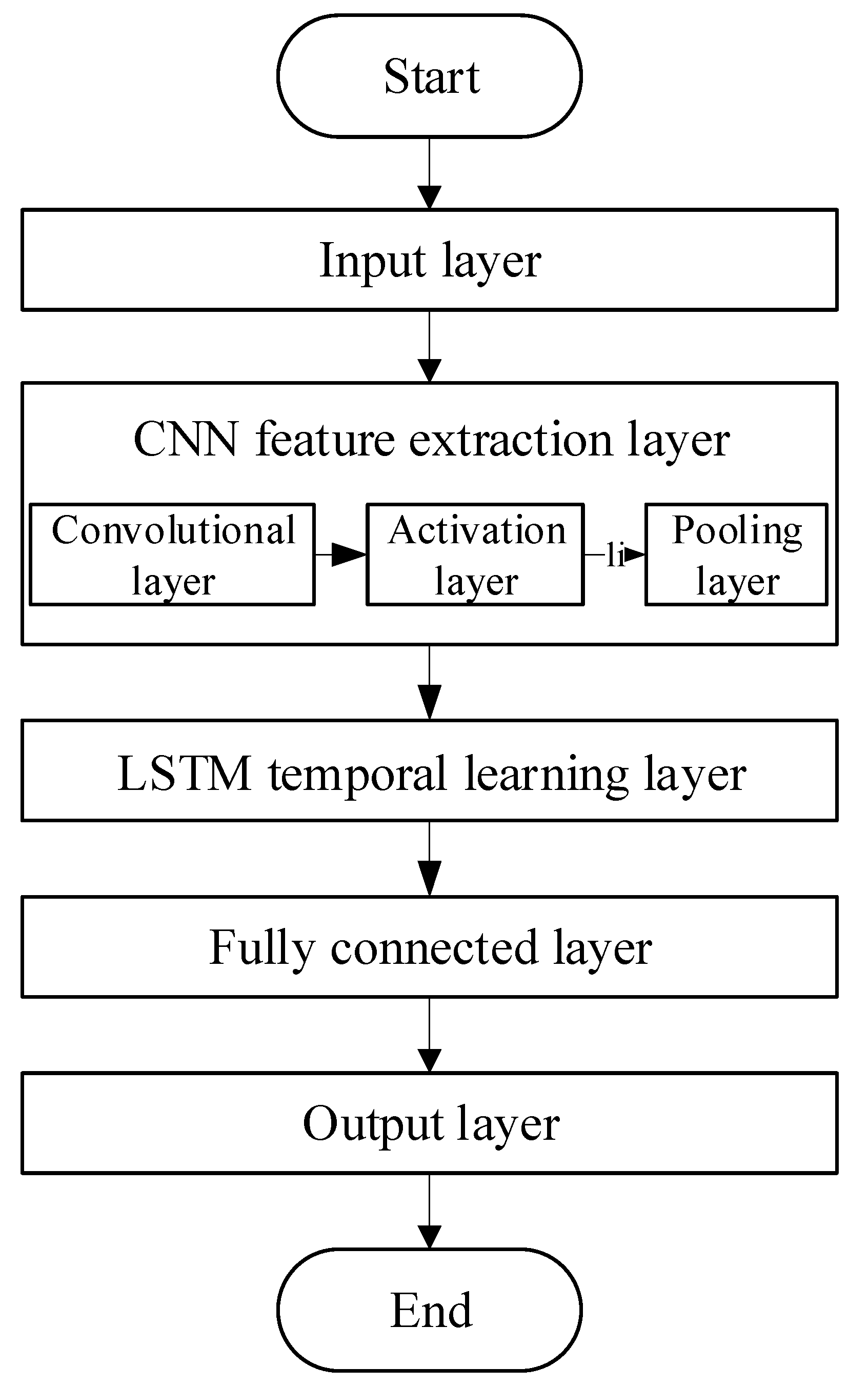
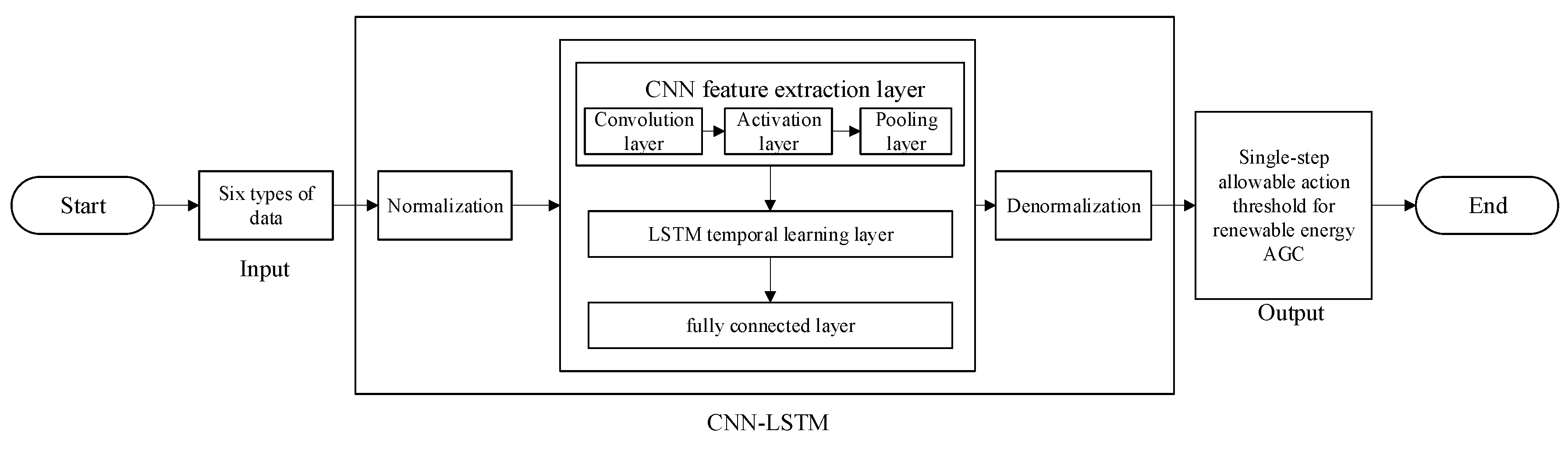
The CNN-LSTM model combines the local feature extraction capability of CNN with the temporal learning capability of LSTM. It is designed for time-series data containing both spatial and temporal dependencies [40,41,42]. The architecture of the proposed neural network is shown in Figure 11 which consists of an input layer, a CNN feature extraction layer, a LSTM temporal learning layer, a fully connected layer, and an output layer. The details of each layer are as follows.

(a)

Input Layer

The input layer is responsible for inputting the normalized time series into the neural network. The time series contains six features: wind power output, photovoltaic power output, thermal power output, system load, and total system inertia.

(b)

CNN Feature Extraction Layer

The CNN feature extraction layer in this paper mainly consists of convolutional layers, activation layers, and pooling layers. A brief introduction is presented in the following.

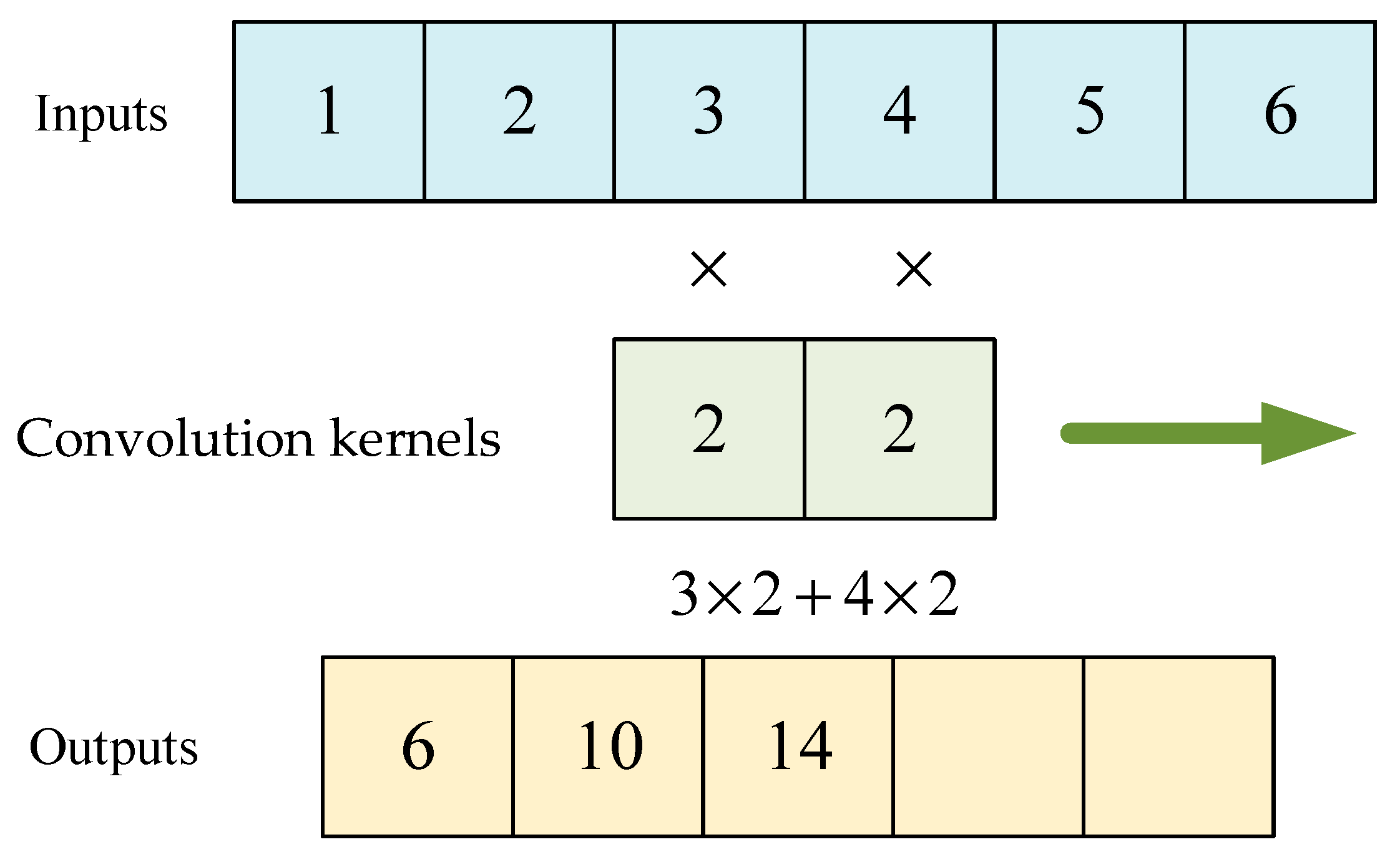
The convolutional layers are used to extract spatial features from time series data [43,44]. The convolution layers slide kernels across the input to extract local dependencies. This process captures fluctuation patterns such as short-term wind variations and the daily cycle of photovoltaic generation. An example of the convolution operation process is shown in Figure 12.

The activation layers enhance the nonlinear representation capability of the network, enabling the model to effectively learn complex patterns and features from the input data. In this model, the activation layer adopts the ReLU function as the activation function. ReLU provides fast convergence and efficient gradient computation. By truncating negative values, it introduces nonlinear breakpoints at each layer, enabling the network to learn more complex mapping relationships, as shown in Equation (17).

$$f(x)=\max (0,x).$$

(17)

The pooling layers perform a dimensionality reduction on the output of the convolutional layers, decreasing the spatial dimensions of feature maps to reduce computational complexity while retaining the most important features. This helps to reduce computation, prevent overfitting, and achieve translation invariance in feature extraction.

(c)

LSTM Temporal Learning Layer

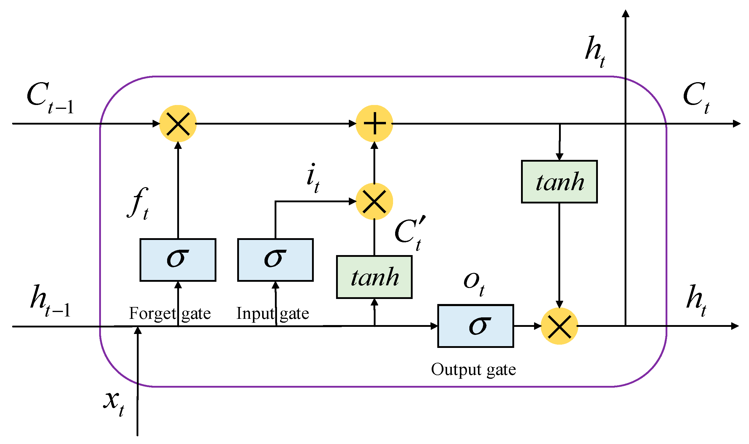
The LSTM temporal learning layer undertakes the core task of sequence learning, and its structure is represented in Figure 13. Based on the local features extracted by the CNN feature extraction layer, it learns temporal dependencies from the time series data, capturing the dynamic variation trends of variables such as generator output and system load [45,46]. It models the relationships among generator output, system inertia, system load, and other factors with the AGC action threshold, thereby determining the single-step action threshold of renewable energy AGC.

When data is fed into the LSTM, it first passes through the forget gate to discard irrelevant information. The calculation is expressed as

$$f_t=\sigma \left(W_f\cdot \left[h_{t-1},x_t\right]+b_f\right),$$

(18)

where $\sigma (x)$ denotes activation function, $h_{t-1}$ denotes the state of the hidden layer at time t − 1, $x_t$ denotes input at time t, and $W_f$ and $b_f$ are the weight matrix and bias.

Then, the model needs to determine what type of information should be updated into the cell state. This process consists of two steps: first, the input gate identifies the information to be updated, denoted as $i_t$; second, the tanh layer is employed to update the information and generates the candidate cell state $C_t^{\prime }$. The calculation formulas for $i_t$ and $C_t^{\prime }$ are given as follows:

$$i_t=\sigma \left(W_i\cdot \left[h_{t-1},x_t\right]+b_i\right);$$

(19)

$$C_t^{\prime }=\tanh \left(W_C\cdot \left[h_{t-1},x_t\right]+b_C\right),$$

(20)

where $i_t$ is the input gate function, $W_i$ and $b_i$ are the weight matrix and bias for $i_t$, and $W_C$ and $b_C$ are the weight matrix and bias for the state of cell.

Next, the outputs of the forget gate and input gate are combined to update the cell state $C_t$, as expressed by

$$C_t=f_t\cdot C_{t-1}+i_t\cdot C_t^{\prime },$$

(21)

where $C_{t-1}$ represents the state of cell at time t − 1.

Finally, the output gate determines the final output, which is calculated as

$$o_t=\sigma \left(W_o\cdot \left[h_{t-1},x_t\right]+b_o\right);$$

(22)

$$h_t=o_t\cdot \tanh \left(C_t\right),$$

(23)

where $o_t$ is the output gate function, and $W_o$ and $b_o$ are the weight matrix and bias for $o_t$.

To enhance the modeling ability without causing overfitting or excessive computational cost, the temporal learning layer employs a two-layer LSTM architecture. The input dimension is set to 32, corresponding to the number of feature maps extracted by the CNN. The hidden layer dimension is set to 64, representing the size of the hidden state at each time step within the LSTM computation. Model parameters, including weight matrices and biases, are updated during training through backpropagation to minimize the loss function and improve prediction accuracy. The Mean Squared Error (MSE) [47,48,49] is adopted as the loss function to quantify the deviation between the predicted and actual values, as expressed in Equation (24).

$$MSE={\displaystyle \frac{1}{n}}{\displaystyle \sum _{i=1}^N({\overline{s}}_i-s_i}{)}^2,$$

(24)

where ${\overline{s}}_i$ denotes the predicted value of the model, $s_i$ denotes actual value, and n denotes the sample size.

(d)

Fully Connected Layer

The fully connected layer in this model is primarily employed to perform a further linear transformation on the features extracted by the LSTM layer, producing the final output. The mathematical expression is given as

$$y=Wx+b,$$

(25)

where W is the weight matrix of the fully connected layer, which performs a weighted summation of the 64-dimensional feature vector obtained from the LSTM computation. b denotes the bias that adjusts the output offset, and y is the final output, corresponding to the single-step allowable action threshold for renewable energy AGC. The fully connected layer consists of a single layer with 64 neurons and 1 output neuron.

(e)

Output Layer

Since the output of the fully connected layer is a normalized threshold, the output layer is responsible for performing inverse normalization on this value to obtain the actual threshold, as shown in Equation (26).

$$y_i=(\max (x)-\min (x))x_i+\min (x).$$

(26)

In Equation (26), $x_i$ represents the i-th normalized action threshold output from the fully connected layer, and $\max (x)$ and $\min (x)$ represent the maximum and minimum single-step allowable action threshold in the dataset, respectively.

3.2.3. The Determination Method for the Single-Step Allowable Action Threshold for Renewable Energy AGC Based on CNN-LSTM

To determine the single-step allowable action threshold for renewable energy, a CNN–LSTM model is employed for real-time threshold calculation based on Section 3.1.3. Photovoltaic output, wind generation output, thermal power output, hydropower output, system load, and total system inertia are used as the input data of CNN–LSTM model and normalized. The simulation data obtained through the model-based method is used to expand the existing data and conduct the model training. Subsequently, CNN is applied to extract local features, and LSTM, with its gating mechanism that effectively captures long-term dependencies and nonlinear temporal patterns, is employed for sequential learning of the extracted features. Finally, a fully connected layer is employed to perform further linear transformation on the LSTM-processed features, and inverse normalization is then conducted to output the single-step allowable action threshold for renewable energy AGC (Figure 14).

The CNN-LSTM model can improve the computational efficiency of threshold determination effectively. However, this data-driven method still faces some limitations in practice, as the accuracy of the neural network’s output threshold heavily depends on the coverage and diversity of the training data. Consequently, when the data distribution changes unexpectedly or under abnormal operating conditions, significant output deviations or even misjudgments may occur. To address this issue, an error-prevention verification method is designed to establish an effective safeguard mechanism for the data-driven threshold determination, enabling the timely detection and blocking of severe deviations in neural network outputs.

3.2.4. Error-Prevention Verification

For each data-driven output of the single-step allowable action threshold $P_{\mathrm{o}d}$ for renewable energy AGC, we use Equation (27) to compute the current area’s threshold. This value serves as the safety threshold for subsequent verification.

$$P_{iNs}=2\ast {\beta }_i\ast \Delta f_{imax}.$$

(27)

Next, compare the absolute value of the data-driven threshold $P_{\mathrm{o}d}$ with the safety threshold $P_{iNs}$ obtained from Equation (27). If the data-driven threshold is smaller than the safety threshold, it passes the verification; otherwise, its output is blocked, and half of the safety threshold (${\beta }_i\ast \Delta f_{imax}$) is directly used as the output. Then, return to the data-driven stage to retrain the CNN-LSTM model by adjusting relevant hyperparameters and increasing training samples.

3.3. Adaptive Threshold Optimization Method

In this study, the data-driven output results are real-time and frequent, so the threshold output results change from time to time. During periods of smooth grid fluctuations, continual threshold updates may hinder dispatchers from making correct decisions. The adaptive piecewise constant approximation (APCA) algorithm and the adaptive threshold adjustment method are designed to balance rapid response and operational efficiency.

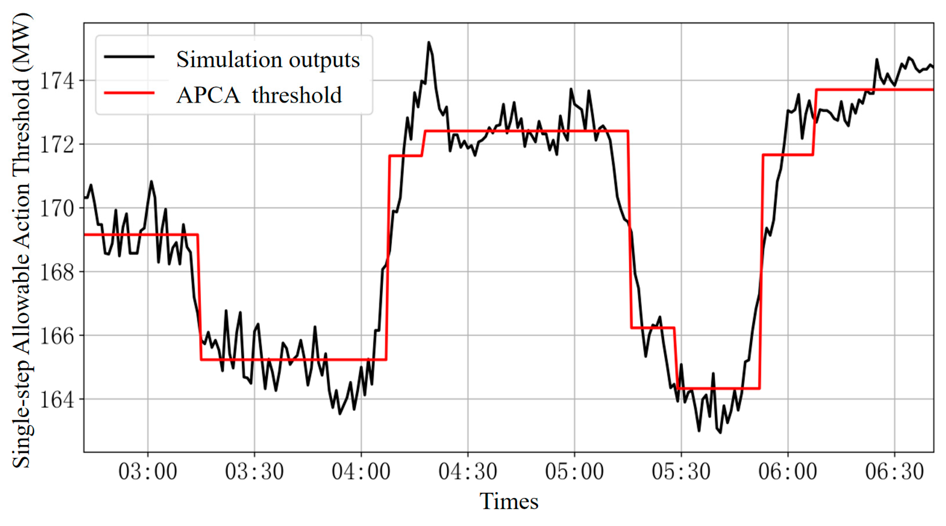
Specifically, the APCA algorithm monitors the fluctuation characteristics of the grid state. When the system operates smoothly, it increases the piecewise interval, keeping the threshold constant for longer periods to reduce unnecessary updates and lower the dispatcher’s workload. When the grid experiences sudden or large variations, the algorithm automatically shortens the interval and updates the threshold more frequently, ensuring timely response to dynamic changes (as shown in Figure 15 in this manuscript).

The adaptive threshold adjustment method further complements this mechanism, which is mainly for extreme scenarios. Under normal conditions, the threshold remains conservative and stable to maintain operational simplicity. However, once extreme or emergency scenarios are detected, the method dynamically enlarges the threshold boundary, allowing renewable resources to respond rapidly and effectively. These two mechanisms achieve a coordinated balance between responsiveness and update efficiency.

3.3.1. Adaptive Threshold Piecewise Method Based on APCA Approach

During periods of smooth grid fluctuations, continual threshold updates may hinder dispatchers from making correct decisions. To address this issue, this paper proposes the adaptive piecewise threshold optimization method based on the APCA (Adaptive Piecewise Constant Approximation) approach [50,51]. This method adjusts the frequency of threshold updates according to the fluctuation characteristics of the system state, reducing the operational burden. An illustrative example is shown in Figure 15. Specifically, it adaptively adjusts the output frequency of the threshold according to the system’s operating condition: when the time-series variation in the grid state is smooth, the corresponding piecewise length is longer; when the fluctuation is more pronounced, the piecewise length becomes shorter. It effectively minimizes the workload of dispatch personnel.

The specific steps of the method are as follows:

(1)

Adaptive Piecewise Parameter Setting: The core parameters of the APCA algorithm are first determined: the maximum piecewise error threshold $\epsilon$, which controls piecewise accuracy (smaller values indicate higher precision), and the minimum piecewise length $l_{min}$, which defines the minimum non-update interval (e.g., 10 min means the threshold is not updated within 10 min). The input data are the time-series of the single-step allowable action thresholds $P_{\mathrm{o}d}$ obtained from Section 3.

(2)

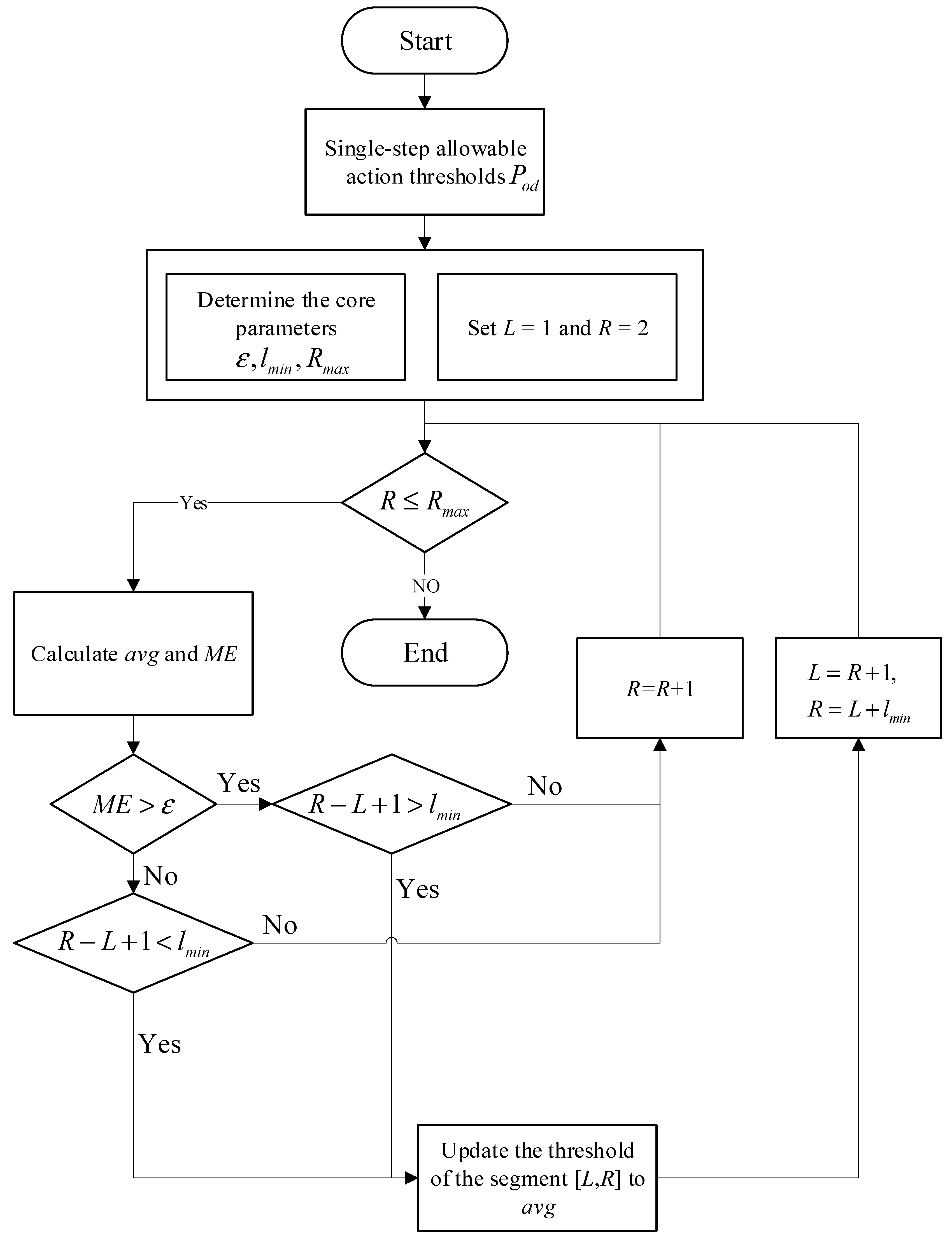
APCA-Based Adaptive Piecewise Calculation: Initialize the piecewise start point $L=1$ and end point $R=2$. Then, calculate the average value avg of $P_{\mathrm{o}d}$ within the current segment $[L,R]$, as expressed in Equation (28):

$$avg={\displaystyle \frac{1}{R-L+1}}{\displaystyle \sum _{k=L}^R{P}_{od}(k)}.$$

(28)

Next, calculate the maximum error $ME$ within the current segment, as expressed in Equation (29):

$$ME=\max \left|P_{od}(k)-a\mathrm{vg}\right|,k\in [L,R].$$

(29)

If $ME\le \epsilon$ and $R-L+1\ge l_{min}$, or $ME>\epsilon$ and $R-L+1<l_{min}$ are satisfied, set the threshold in this segment to $avg$, record the segment $[L,R]$, and update $L=R+1$ and $R=L+l_{min}$; otherwise, set $R=R+1$. Repeat the above process until $R$ reaches the maximum value $R_{max}$. The resulting sequence is the adaptively piecewise optimized threshold series $P_{odk}$; the detailed procedure is illustrated in Figure 16.

3.3.2. Adaptive Threshold Adjustment Under Extreme Scenarios

The above obtained single-step allowable action threshold for renewable energy AGC primarily applies to normal operating conditions. However, under extreme scenarios, strictly limiting this threshold would constrain the rapid regulation capability of renewable energy sources, preventing them from contributing effectively to the rapid stabilization of the power system. To address this issue, this paper proposes an adaptive adjustment of the single-step allowable action threshold for renewable energy AGC under extreme scenarios. Specifically, it integrates meteorological warning systems (to detect extreme weather events such as typhoons, severe sandstorms, and heavy rainfall) and power system stability systems (to identify grid faults such as DC pole blocking and line tripping) to achieve identification of two categories of extreme scenarios. The detailed identification methods for these extreme scenarios can be found in [52,53,54,55].

If the current scenario is identified as a normal operating condition, the threshold is directly applied. Otherwise, the single-step allowable action threshold of renewable energy AGC ($P_{odk}$) is expanded by a factor of ten, fully enhancing the rapid regulation capability of renewable energy AGC.

4. Results and Discussion

In this section, we demonstrate the superior performance of our proposed single-step allowable action threshold determination method. The specific experimental process and results are as follows.

4.1. Experiment Settings

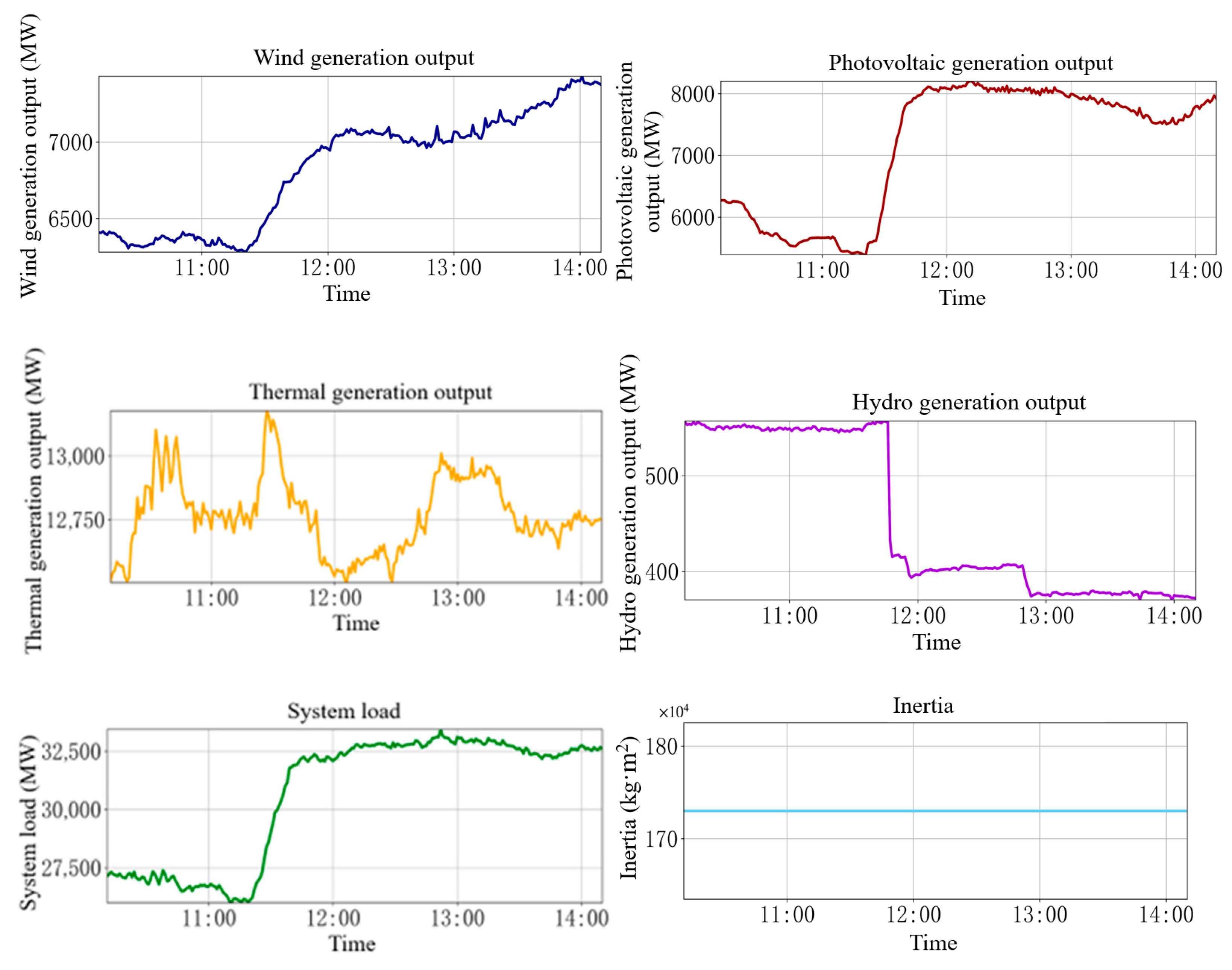
To evaluate the effectiveness of the dynamic threshold determination, a dataset from a provincial power system in China is employed, including photovoltaic, wind, thermal, and hydro-generation outputs, as well as system load and inertia. The dataset consists of 36 groups, each covering 24 h with one-minute sampling intervals; partial data is as shown in

Table 2. Relevant AGC data of the test system.

Times	Wind Generation Output (MW)	Photovoltaic Generation Output (MW)	Thermal Generation Output (MW)	Hydro-Generation Output (MW)	System Load (MW)	Inertia (104 kg·m2)
10:39	3661	6217	21,017	654	33,581	128
10:40	3658	6273	21,053	651	33,721	128
10:41	3665	6271	21,073	652	33,841	128
10:42	3654	6240	21,101	651	33,702	128
10:43	3642	6232	21,061	654	33,631	128
10:44	3660	6234	21,049	652	33,547	128
10:45	3667	6259	21,023	654	33,687	128
10:46	3674	6255	20,974	653	33,530	128

.

Following the core principle of “data-driven dominant, model-based assisted,” the model first determines the allowable action threshold for renewable energy AGC over a given period using the model-driven approach. This result is then used to train the data-driven model that learns the mapping relationship between system state variables and the threshold. Finally, the threshold is adaptively determined based on real-time input data.

4.2. The Experiment of Model-Based Method

4.2.1. Parameter Settings

In this chapter, three representative scenarios with different renewable energy penetration levels are selected from 36 test cases to evaluate the generalization capability of the proposed model. This experiment was conducted based on the AGC model established in Section 3.1 to perform the simulation analysis and determine the single-step allowable action threshold. The specific settings of the model parameters are as presented in

Table 3. The specific settings of the model parameters.

Parameters	Value
$D$	1
$R$	2.4
$T_G$	0.2
$T_{CH}$	0.3
$T_{HP}$	0.25
$T_{RH}$	10
$K_P$	5.6
$K_n$	0.28
$K_i$	1.2
$T_r$	5
$T_h$	28.75
$T_w$	1
$b_p$	0.06

.

Assuming an allowable frequency deviation range of 0.06 Hz to 0.08 Hz, with the maximum and minimum outputs of new energy units in the dataset being 15,352 MW and 2137 MW, respectively, the coefficient is thus set as $K=1.51\times {10}^{-6}$ and $b=0.0568$. Set $\min =0$, $\max =0.2$, and $\epsilon =1\times {10}^{-4}$.

4.2.2. Experimental Results and Discussion

To verify the generalization capability of the proposed model, three representative scenarios with different levels of renewable energy penetration—6%, 27%, and 52%—were selected for analysis. The specific results and corresponding discussions are presented as follows.

(1)

Scenario I (the level of renewable energy penetration is 6%)

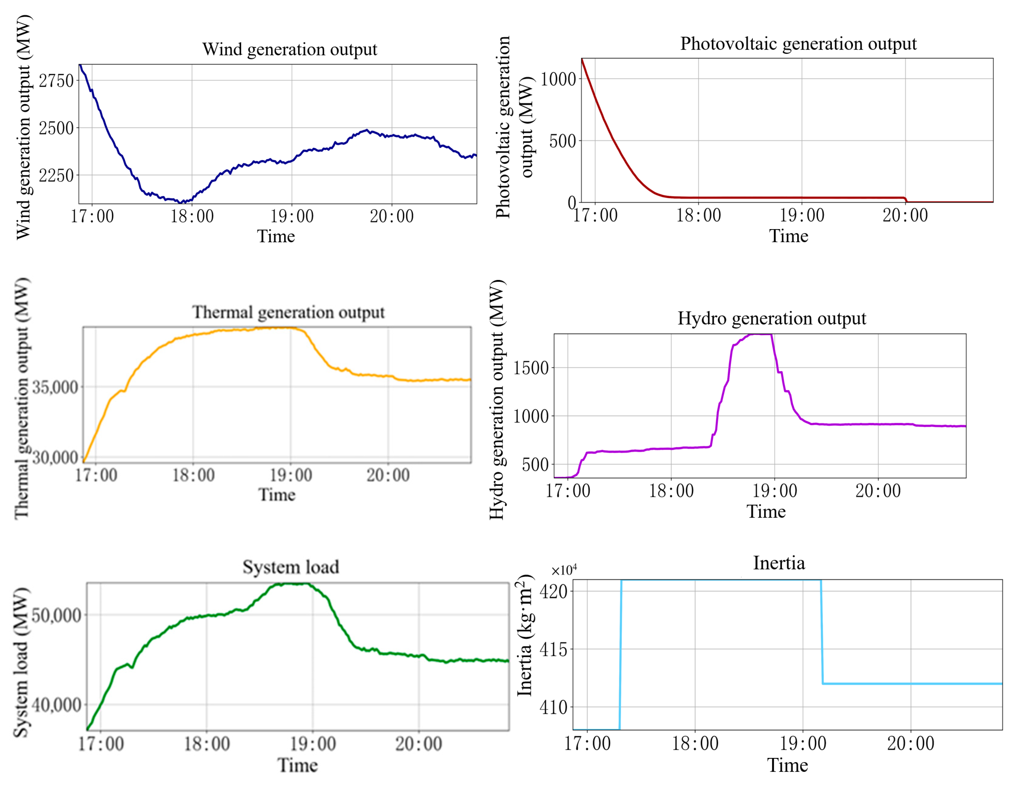
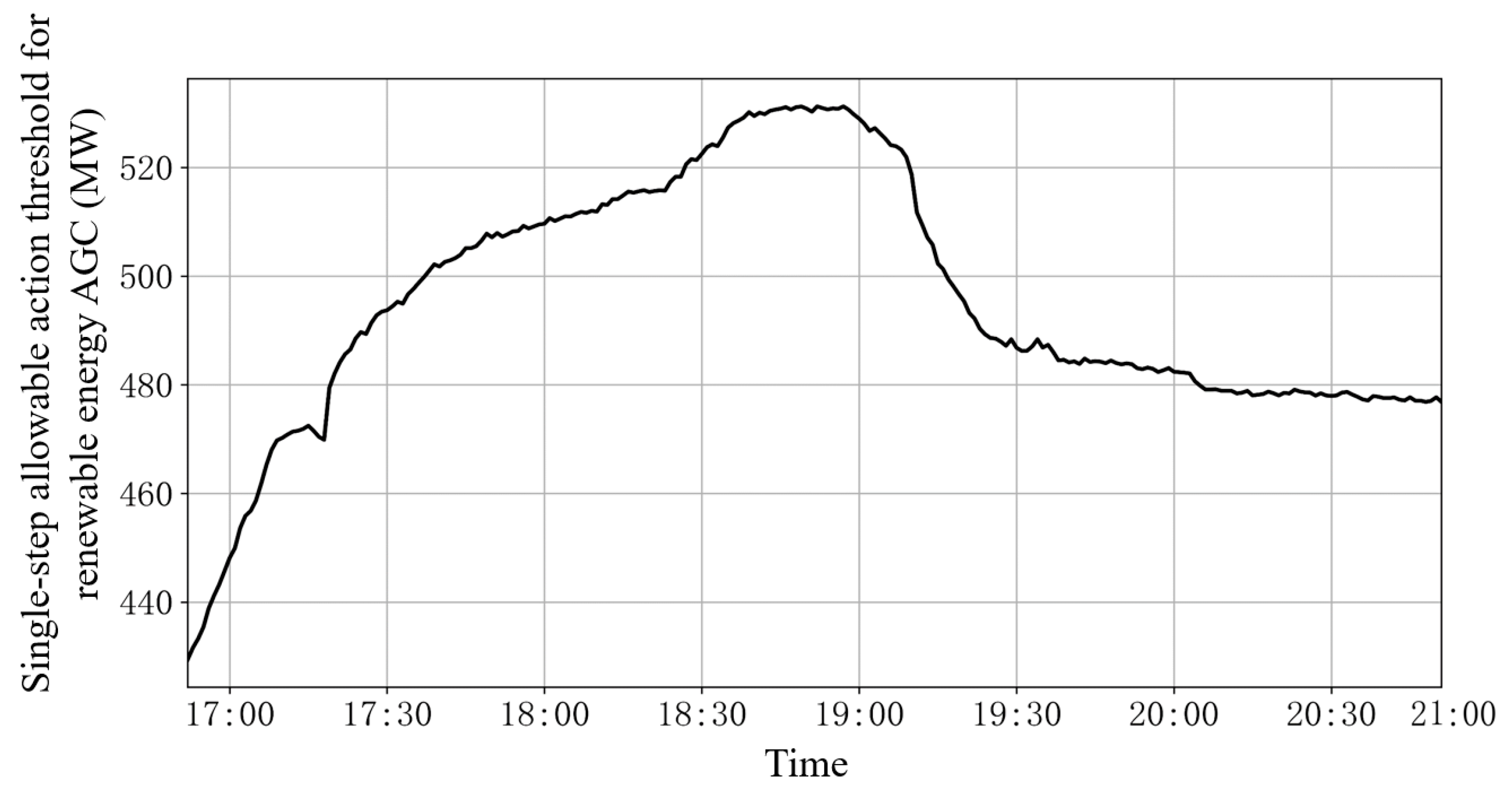
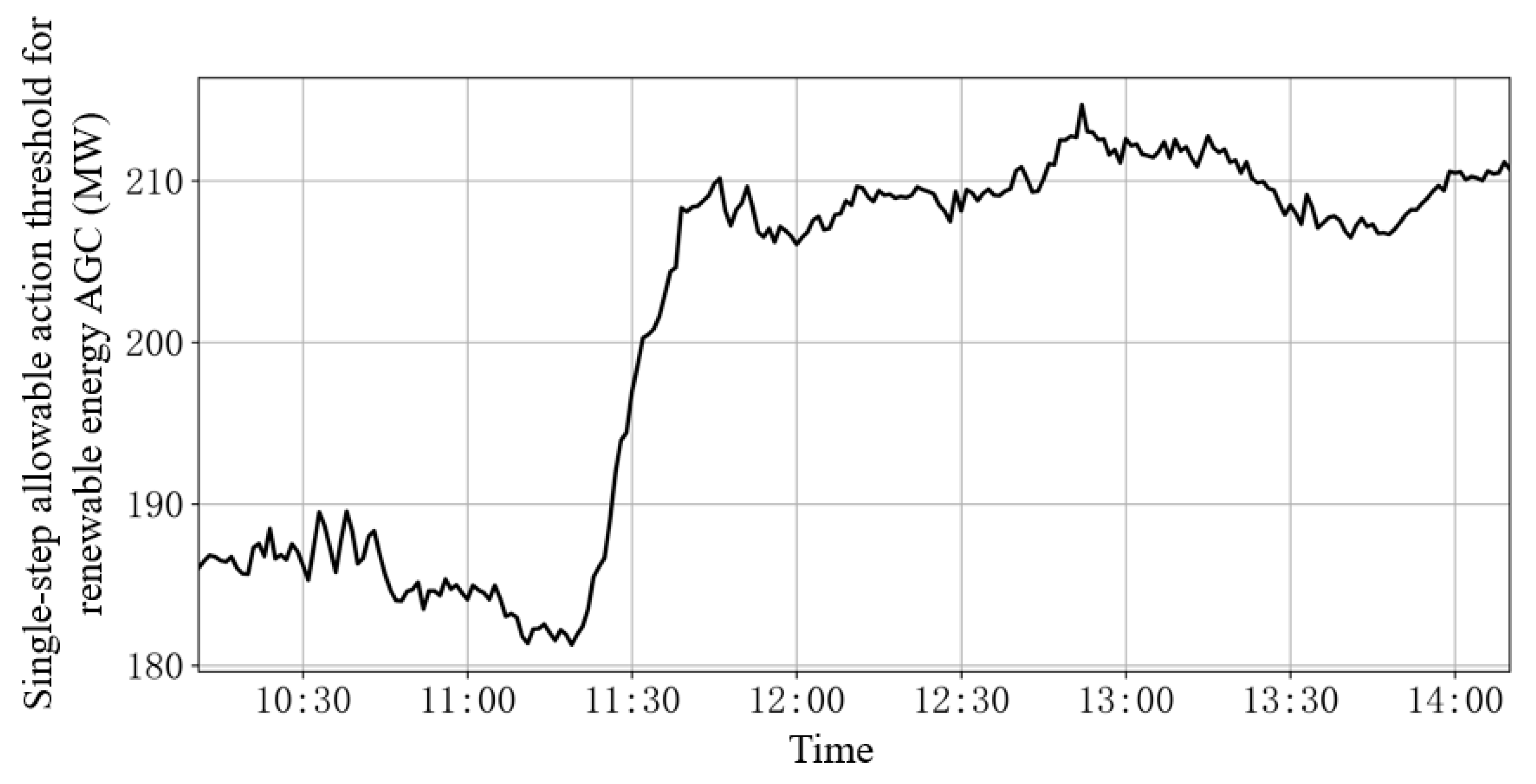
In Scenario 1, the data and the resulting single-step allowable action thresholds are shown in Figure 17 and Figure 18, respectively. The threshold curve follows the trends of system load and thermal generation. Renewable generation is low in this case and has little influence on the threshold (average 2471 MW). The region is dominated by thermal power units, leading to a strong correlation between total load and thermal output. Since the frequency deviation coefficient is positively related to load variations and generator output, the threshold curve closely follows the trajectories of system load and the thermal generator.

(2)

Scenario II (the level of renewable energy penetration is 27%)

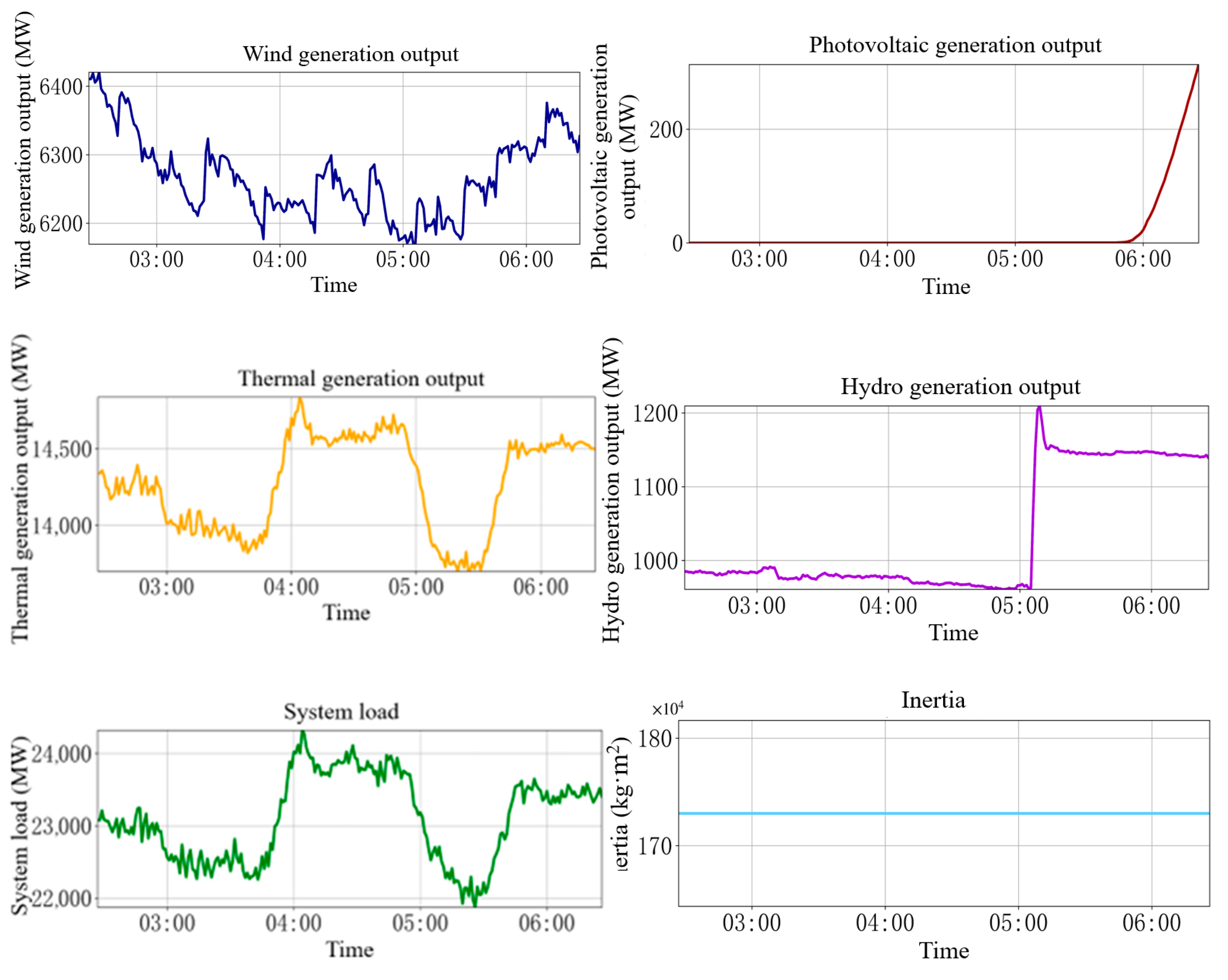
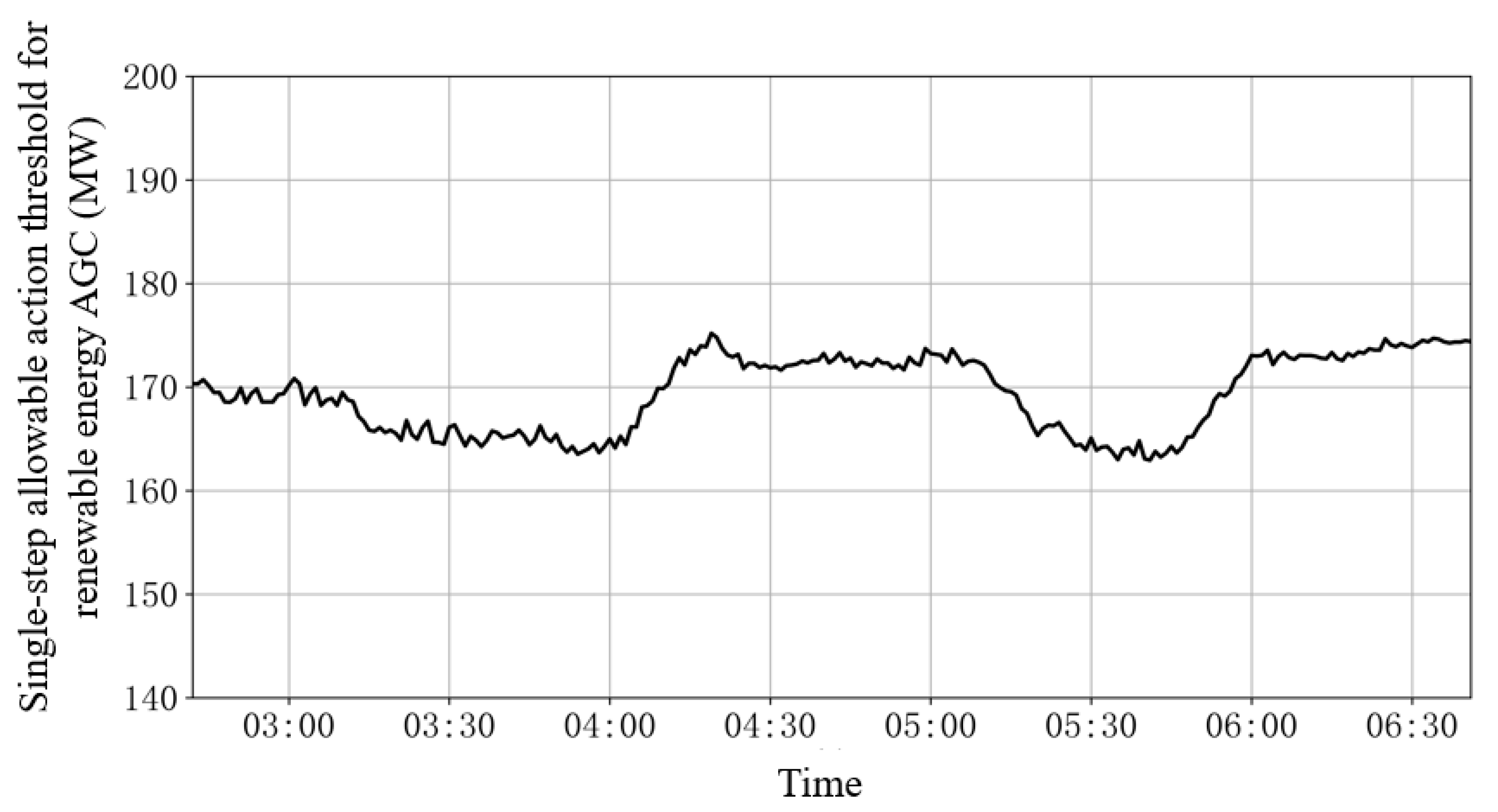
In Scenario II, the system operates during the early-morning period, where system inertia, the frequency–power characteristic coefficient (B coefficient), and the maximum allowable frequency deviation remain relatively low with minimal fluctuation. Consequently, the resulting single-step allowable action threshold is also lower than that in other scenarios and exhibits a generally stable pattern (Figure 19 and Figure 20).

(3)

Scenario III (the level of renewable energy penetration is 52%)

In Scenario III, the renewable energy generation output remains at a high level (averaging 13,991 MW and a maximum–minimum difference of 3679 MW). This leads to a large fluctuation in the allowable maximum frequency deviation. Meanwhile, conventional generation remains stable with little variation, implying a nearly constant B coefficient and unchanged system inertia. Therefore, the single-step allowable action threshold closely follows the renewable energy generation output, clearly demonstrating that the allowable frequency deviation plays a dominant role in determining the single-step allowable action threshold for renewable energy AGC (Figure 21 and Figure 22).

Although few studies have examined the single-step allowable action threshold for AGC and comparable datasets are limited, the simulation results show that the proposed model-based method provides effectiveness threshold values. By comprehensively accounting for multiple influencing factors and validating performance through a constructed simulation system, the model successfully determines reasonable allowable action thresholds under various representative scenarios. The obtained thresholds align with practical grid operation experience, confirming the validity and applicability of the proposed method, and offering a valuable reference for error operation detection and prevention in dispatching systems.

4.3. The Experiment of Data-Driven Method

The experimental data employed in this section are derived from AGC operation records of a provincial power grid in China (as shown in Table 2), along with the single-step allowable action thresholds for renewable energy AGC determined through the simulations presented in Section 4.2.

The experiments in this section are implemented in Python 3.7 using the PyCharm (PyCharm2024) integrated development environment. The computing platform is equipped with an Intel i7-12700H processor (Intel Corporation, Santa Clara, CA, USA), an RTX-2050 GPU (NVIDIA Corporation, Santa Clara, CA, USA), 16 GB of RAM, and 8 GB of video memory. The three representative scenarios described in Section 4.2 are used as the test set, while the remaining data are employed for model training. The root mean squared error (RMSE) and mean absolute error (MAE) [56,57,58,59] are employed as the index, RMSE and MAE is shown in Equations (30) and (31).

$$RMSE=\sqrt{{\displaystyle \frac{1}{n}}{\displaystyle \sum _{i=1}^N({\overline{s}}_i-s_i}{)}^2};$$

(30)

$$MAE={\displaystyle \frac{1}{n}}{\displaystyle \sum _{i=1}^n\left|y_i-{\overline{y}}_i\right|},$$

(31)

where $y_i$ denotes the i-th actual action threshold, and ${\overline{y}}_i$ denotes the i-th action threshold of the neural network output.

To further evaluate the superiority of the proposed data-driven method, comparative experiments were conducted by replacing the model with another neural network. Scenario I was selected as the test case, and four alternative models were implemented for comparison: (1) CNN-based [60] threshold determination for renewable energy AGC, (2) LSTM-based [61] threshold determination for renewable energy AGC, (3) Transformer-based [62] threshold determination for renewable energy AGC, and (4) Support Vector Regression (SVR)-based [63] threshold determination for renewable energy AGC.

Table 4. Experimental parameter results.

Parameters	RMSE	MAE
CNN	30.23	27.42
LSTM	9.12	7.33
Transformer	10.16	8.03
SVR	47.68	38.32
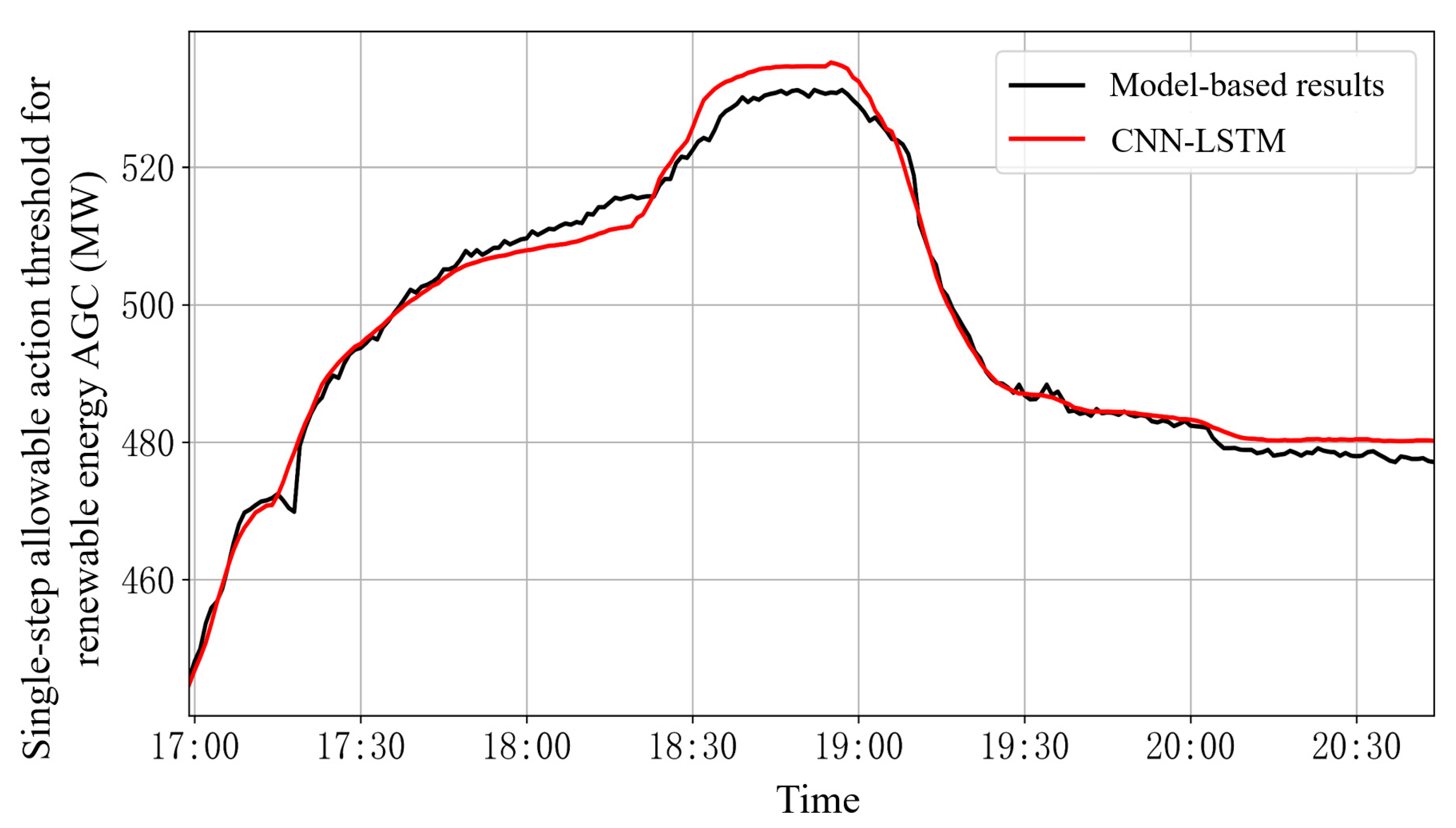
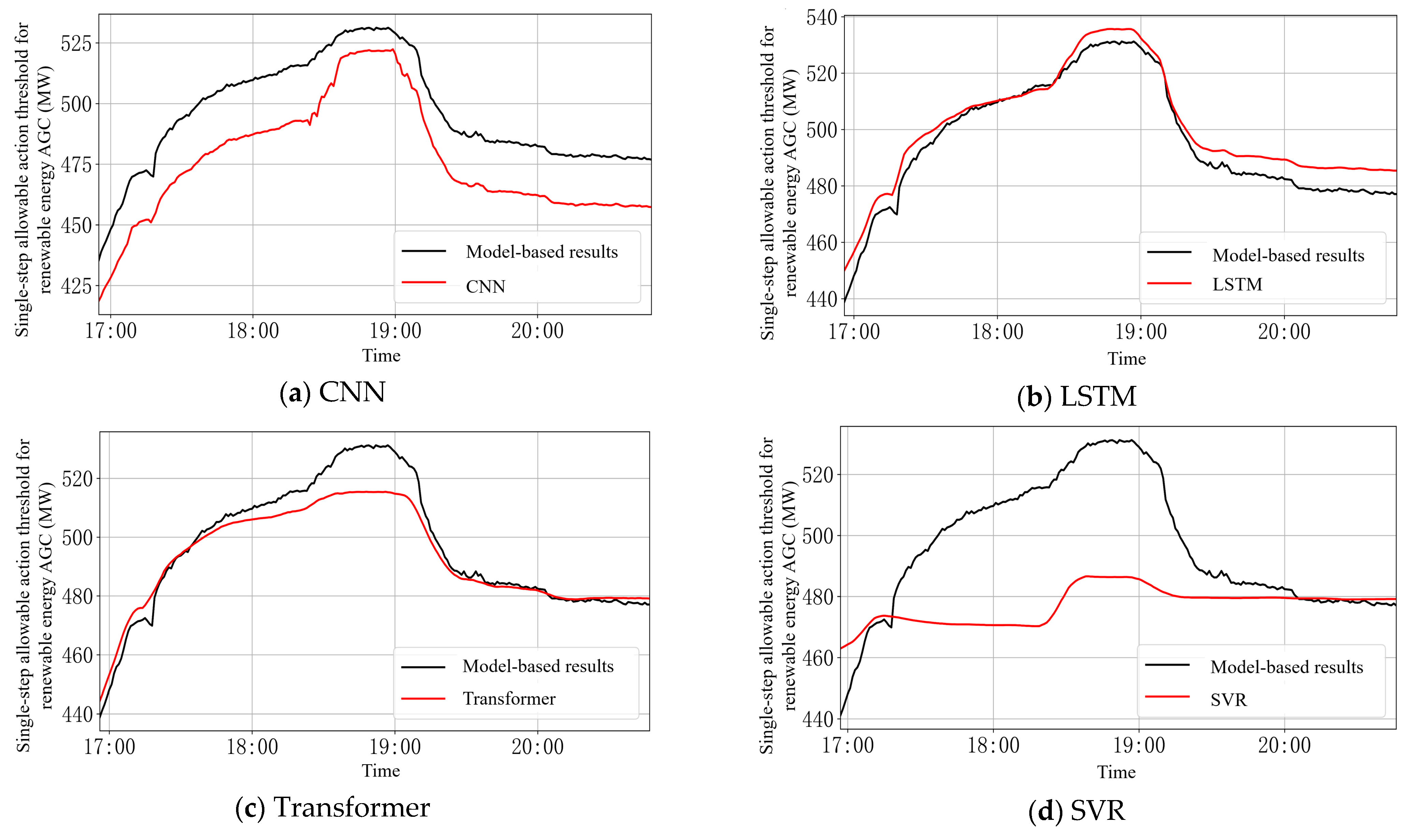
The model proposed in this study	4.09	3.18

presents the evaluation metrics of all the comparative experiments. Figure 23 shows the results of the proposed model; Figure 24 displays the results of baseline models. The detailed analysis is as follows.

(1)

Overall effectiveness of the proposed model.

The proposed neural network achieves superior accuracy, with an RMSE of 4.09 and an MAE of 3.18. Moreover, Figure 24 indicates consistent performance across different scenarios, demonstrating strong generalization capability. Compared with Transformer, RMSE and MAE are reduced by 60%, and compared with SVR, the reductions reach 93% and 92%, respectively. This advantage is mainly attributed to the following reasons: (a) The dataset samples contain only 4 h per scenario, making sequence lengths relatively short; thus, Transformer, which relies on long-range dependencies, performs worse. In contrast, the AGC threshold determination is dominated by local operating characteristics of the power grid, which CNN-LSTM captures more effectively. (b) SVR, as a traditional regression method, is limited in handling high-dimensional and highly nonlinear relationships, whereas AGC thresholds exhibit a strong nonlinear dependence on generator output, system inertia, and load. CNN-LSTM provides more expressive nonlinear temporal modeling, and hence significantly outperforms SVR.

(2)

Necessity of the CNN feature extraction layer.

The proposed model outperforms the LSTM-only model, with reductions of 55% in RMSE and 57% in MAE. This confirms that the CNN layer effectively extracts local temporal features (e.g., short-term trends and local correlations) from the grid operating data, enabling the LSTM to better capture dynamic evolution and improving model prediction accuracy.

(3)

Necessity of the LSTM temporal learning layer.

The proposed model also surpasses the CNN-only model, reducing RMSE by 86% and MAE by 88%. Benefiting from its gated architecture, LSTM retains long-term information and captures temporal dependencies that CNN alone cannot model, validating the essential role of the temporal learning layer.

(4)

Verification of model rapidity.

As shown in

Table 5. The runtime of the model-based and CNN-LSTM methods.

Model-Based Approach Runtime	CNN-LSTM Runtime (ms)
8866	23

, the model-based threshold determination in Section 3 requires an average computation time of 8866 ms, whereas the proposed CNN-LSTM approach achieves an average response time of only 23 ms, representing a 99.7% reduction. This remarkable improvement confirms that the proposed threshold determination method fully satisfies the fast-response requirement of abnormal operation detection and assists in error operation prevention for renewable energy AGC systems.

4.4. Experiment Using the Adaptive Threshold Piecewise Method

The APCA algorithm keeps the threshold within an acceptable approximation error. At the same time, it reduces update frequency and stabilizes changes in the threshold. RMSE and the compression ratio (CR) were employed to evaluate the performance of the proposed segmentation method, as defined below:

$$CR={\displaystyle \frac{M}{N}},$$

(32)

where M is the number of input data points and N is the number of segments. This parameter reflects the update frequency of the single-step allowable action threshold, where a larger value indicates a slower update rate.

After extensive experiments and testing, the maximum allowable error within each segment was set as $\epsilon =7$. Furthermore, to effectively constrain the update frequency of the single-step action threshold, the minimum segment length was set as $\delta =10$, ensuring that the threshold was updated no more frequently than once every 10 min.

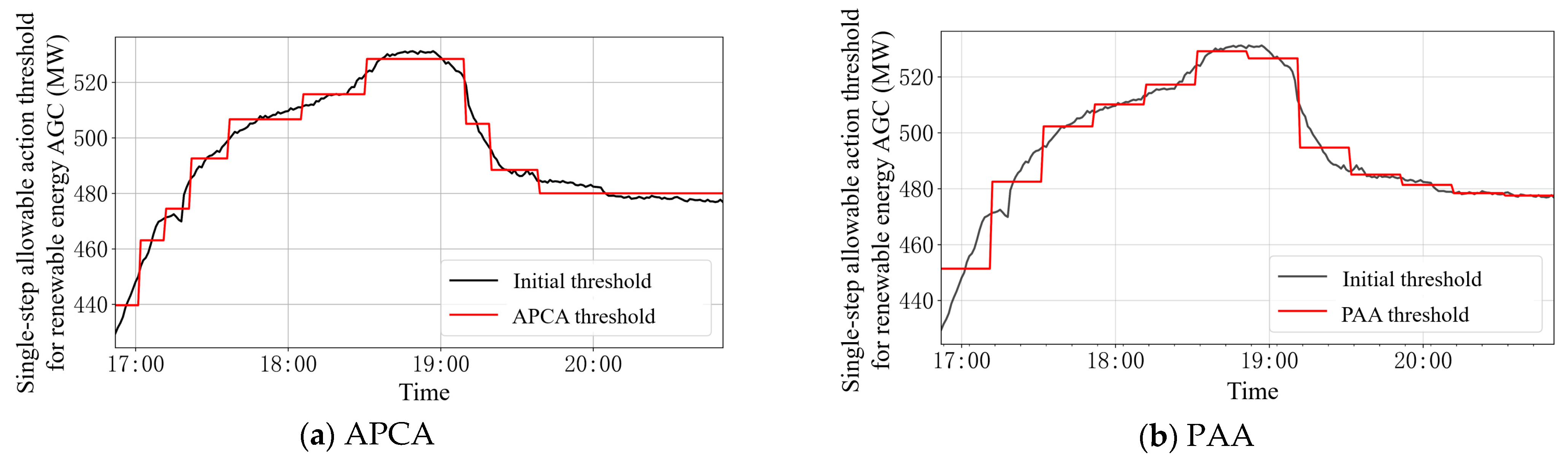
The Piecewise Aggregate Approximation (PAA) algorithm was employed as a baseline for comparison with the APCA algorithm [51]. PAA divides the action-threshold time series into equal-length segments, and each segment is represented by a constant value. In contrast, APCA divides the time series into variable-length segments, while still using a constant value to represent each segment. The results are as follows:

In

Table 6. The experimental index results of the PAA and APCA algorithms.

Method	RMSE	CR
APCA	2.60	48.00
PAA	2.98	20.00

and Figure 25, it is clear that the APCA-based threshold segmentation algorithm achieves a 13% lower RMSE compared with PAA, while increasing the compression ratio by 140%. These experimental results demonstrate that the proposed algorithm effectively reduces the update frequency while maintaining low approximation error, thereby validating its superiority and reliability.

4.5. Further Work

Despite its effectiveness, the proposed method still has several limitations. In the current determination of the single-step allowable action threshold for renewable energy AGC, only conventional generating units are considered in frequency regulation. The impact of renewable units directly participating in frequency response is not yet included. Future work will focus on developing a threshold determination method under scenarios where renewable units also contribute to frequency regulation. In the data-driven threshold determination method, the renewable energy AGC thresholds used for training are derived from simulation. Future studies may incorporate real-world field measurements collected under different grid conditions and operational scenarios to replace simulated data. This will further improve model adaptability and generalization performance in practical applications, enhancing the reliability and engineering applicability of the proposed approach.

It is worth noting that energy storage systems also provide fast frequency responses and their total capacity influences system behavior. Their aggregate capacity can influence the system’s frequency response characteristics similarly to renewable generation. In our manuscript, the proposed method is implemented only at the AGC master station, and no modifications are made to AGC substations or to the control systems of any generating units or storage systems. Although the present work focuses on the total renewable generation participating in AGC, the same threshold-determination framework can be extended to incorporate the aggregated behavior of storage systems. A detailed treatment of storage participation will be considered as part of our future work. At present, a complete labor–cost assessment has not yet been carried out, and this will be an important direction for future work. We have added corresponding statements to the revised manuscript.

5. Conclusions

In this paper, we propose a single-step allowable action threshold determination method for renewable energy AGC using model-based and data-driven approaches. The model-driven approach explicitly incorporates system dynamics and operational constraints, generating physically interpretable thresholds. Based on these results, a CNN-LSTM neural network is trained to achieve efficient, real-time threshold determination. To ensure the safety of systems, an error-prevention validation is further introduced to avoid risky outputs caused by uncertainty in the data-driven method. In addition, an adaptive piecewise constant approximation algorithm is employed to reduce threshold update frequency and the burden for dispatchers. Finally, an adaptive threshold adjustment mechanism under extreme scenarios is introduced. When extreme operational conditions are detected, the output threshold is adaptively extended to fully utilize the fast frequency-regulation capability of renewable resources. Experimental results across multiple renewable penetration scenarios demonstrate the high accuracy, generalizability, and high computational efficiency of this method.

References

1. Pal, P.; Behera, R.K.; Muduli, U.R. Eliminating current sensor dependencies in dab converters using a luenberger observer-based hybrid approach. IEEE Trans. Ind. Appl. 2024, 60, 6380–6392. [Google Scholar] [CrossRef]
2. Saxena, A.; Shankar, R.; Al Zaabi, O.; Al Hosani, K.; Muduli, U.R. Fuzzy rule-based adaptive virtual inertia control for enhancing multi-region micro-grid dynamic response. In Proceedings of the 2023 IEEE IAS Global Conference on Renewable Energy and Hydrogen Technologies (GlobConHT), Malé, Maldives, 11–12 March 2023; pp. 1–6. [Google Scholar] [CrossRef]
3. Saxena, A.; Shankar, R.; El-Saadany, E.F.; Kumar, M.; Al Zaabi, O.; Al Hosani, K.; Muduli, U.R. Intelligent Load Forecasting and Renewable Energy Integration for Enhanced Grid Reliability. IEEE Trans. Ind. Appl. 2024, 60, 8403–8417. [Google Scholar] [CrossRef]
4. Peddakapu, K.; Mohamed, M.R.; Srinivasarao, P.; Arya, Y.; Leung, P.K.; Kishore, D.J.K. A State-of-the-Art Review on Modern and Future Developments of AGC/LFC of Conventional and Renewable Energy-Based Power Systems. Renew. Energy Focus 2022, 43, 146–171. [Google Scholar] [CrossRef]
5. Xiang, M.; Yang, Z.; Yu, J. Hierarchical AGC dispatch with detailed modeling of energy storage system behaviors. IEEE Trans. Power Syst. 2023, 38, 1689–1701. [Google Scholar] [CrossRef]
6. Wang, Y.; Wan, C.; Zhou, Z.; Zhang, K.; Botterud, A. Improving deployment availability of energy storage with data-driven AGC signal models. IEEE Trans. Power Syst. 2018, 33, 4207–4217. [Google Scholar] [CrossRef]
7. Bevrani, H.; Hiyama, T. Intelligent Automatic Generation Control; CRC Press: New York, NY, USA, 2011. [Google Scholar] [CrossRef]
8. Wu, Z.; Gao, W.; Gao, T.; Yan, W.; Zhang, H.; Yan, S.; Wang, X. State-of-the-Art Review on Frequency Response of Wind Power Plants in Power Systems. J. Mod. Power Syst. Clean Energy 2018, 6, 1–16. [Google Scholar] [CrossRef]
9. Qiu, Y.; Lin, J.; Liu, F.; Dai, N.; Song, Y. Continuous Random Process Modeling of AGC Signals Based on Stochastic Differential Equations. IEEE Trans. Power Syst. 2021, 36, 4575–4587. [Google Scholar] [CrossRef]
10. Xi, L.; Yu, L.; Xu, Y.; Wang, S.; Chen, X. A Novel Multi-Agent DDQN-AD Method-Based Distributed Strategy for Automatic Generation Control of Integrated Energy Systems. IEEE Trans. Sustain. Energy 2019, 11, 2417–2426. [Google Scholar] [CrossRef]
11. Xu, Y.; Parisio, A.; Li, Z.; Dong, Z.; Ding, Z. Optimization-Based Ramping Reserve Allocation of BESS for AGC Enhancement. IEEE Trans. Power Syst. 2023, 39, 2491–2505. [Google Scholar] [CrossRef]
12. Ondar, A.M.; Tremyasov, V.A.; Kenden, K.V. Analyzing the Risk Management of Renewable Energy Use. In Proceedings of the 2025 International Conference on Industrial Engineering, Applications and Manufacturing (ICIEAM), Sochi, Russian, 24 August 2025; pp. 183–187. [Google Scholar] [CrossRef]
13. Spain Blackout Reveals Limits of Renewable Solar and Wind Energy. Available online: https://www.independent.co.uk/climate-change/news/spain-blackout-renewable-energy-solar-wind-b2742000.html (accessed on 20 October 2025).
14. 2025 Iberian Peninsula Blackout. Available online: https://en.wikipedia.org/wiki/2025_Iberian_Peninsula_blackout#cite_note-ferris-9 (accessed on 20 October 2025).
15. Du, F.; Zhang, M.; Zhu, K.; Jiang, D. Error Prevention Adaptive Optimization Model for Power Dispatch under Time Redundancy Control. Electr. Eng. 2024, 106, 7579–7586. [Google Scholar] [CrossRef]
16. Taheri, B.; Safdarian, A.; Moeini-Aghtaie, M.; Lehtonen, M. Enhancing Resilience Level of Power Distribution Systems Using Proactive Operational Actions. IEEE Access 2019, 7, 137378–137389. [Google Scholar] [CrossRef]
17. Zhukabayeva, T.; Pervez, A.; Mardenov, Y.; Othman, M.; Karabayev, N.; Ahmad, Z. A Traffic Analysis and Node Categorization-Aware Machine Learning-Integrated Framework for Cybersecurity Intrusion Detection and Prevention of WSNs in Smart Grids. IEEE Access 2024, 12, 91715–91733. [Google Scholar] [CrossRef]
18. Hussain, F.; Abbas, G.S.; Pires, I.M.; Tanveer, S.; Fayyaz, U.U.; Garcia, N.M.; Shah, G.A.; Shahzad, F. A Two-Fold Machine Learning Approach to Prevent and Detect IoT Botnet Attacks. IEEE Access 2021, 9, 163412–163430. [Google Scholar] [CrossRef]
19. Laghari, S.U.A.; Manickam, S.; Al-Ani, A.K.; Rehman, S.U.; Karuppayah, S. SECS/GEMsec: A Mechanism for Detection and Prevention of Cyber-Attacks on SECS/GEM Communications in Industry 4.0 Landscape. IEEE Access 2021, 9, 154380–154394. [Google Scholar] [CrossRef]
20. Zhang, Q.; Li, F.; Zhao, J.; She, B. False Data Injection Attack and Corresponding Countermeasure in Multienergy Systems. IEEE Trans. Power Syst. 2024, 39, 3537–3547. [Google Scholar] [CrossRef]
21. Kuang, M.; Tian, Y.; Liu, Q.; Zhao, M.; Wu, X. A Review of Control Strategies for Automatic Generation Control in Power Systems with Renewable Energy. Prog. Energy 2024, 6, 022001. [Google Scholar] [CrossRef]
22. Liu, D.; Wu, Y.; Kang, Y.; Li, C.; Ji, X.; Zhang, X. Graph Convolution Network for Real-Time AGC Dispatch with High-Penetration Renewable Energy. CSEE J. Power Energy Syst. 2023, 1–11. [Google Scholar] [CrossRef]
23. Debbarma, L.; Debbarma, S.; Roy, K.; Roy, S.D.; Singh, P.P. Joint Contribution of RTEM and AGC System for Frequency Stabilisation in Renewable Energy Integrated Power System. IET Energy Syst. Integr. 2024, 6, 498–511. [Google Scholar] [CrossRef]
24. Hossain, R.R.; Yin, T.; Du, Y.; Huang, R.; Tan, J.; Yu, W.; Liu, Y.; Huang, Q. Efficient Learning of Power Grid Voltage Control Strategies via Model-Based Deep Reinforcement Learning. Mach. Learn. 2024, 113, 2675–2700. [Google Scholar] [CrossRef]
25. Han, D.; Ma, J.; He, R.M.; Dong, Z.Y. A Real Application of Measurement-Based Load Modeling in Large-Scale Power Grids and Its Validation. IEEE Trans. Power Syst. 2009, 24, 1756–1764. [Google Scholar] [CrossRef]
26. Mortazavian, S.; Mohamed, Y.A.R.I. Analysis and Augmented Model-Based Control Design of Distributed Generation Converters with a Flexible Grid-Support Controller. IEEE Trans. Power Electron. 2018, 34, 6369–6387. [Google Scholar] [CrossRef]
27. Yang, Y.; Yang, Z.; Yu, J.; Zhang, B.; Zhang, Y.; Yu, H. Fast Calculation of Probabilistic Power Flow: A Model-Based Deep Learning Approach. IEEE Trans. Smart Grid 2019, 11, 2235–2244. [Google Scholar] [CrossRef]
28. Strielkowski, W.; Vlasov, A.; Selivanov, K.; Muraviev, K.; Shakhnov, V. Prospects and Challenges of the Machine Learning and Data-Driven Methods for the Predictive Analysis of Power Systems: A Review. Energies 2023, 16, 4025. [Google Scholar] [CrossRef]
29. Weng, Y.; Negi, R.; Faloutsos, C.; Ilić, M.D. Robust Data-Driven State Estimation for Smart Grid. IEEE Trans. Smart Grid 2016, 8, 1956–1967. [Google Scholar] [CrossRef]
30. Oh, S.; Kong, J.; Choi, M.; Jung, J. Data-Driven Prediction Method for Power Grid State Subjected to Heavy-Rain Hazards. Appl. Sci. 2020, 10, 4693. [Google Scholar] [CrossRef]
31. Jaleeli, N.; VanSlyck, L.S.; Ewart, D.N.; Fink, L.H.; Hoffmann, A.G. Understanding Automatic Generation Control. IEEE Trans. Power Syst. 1992, 7, 1106–1122. [Google Scholar] [CrossRef]
32. Muduli, R.; Jena, D.; Moger, T. Application of Reinforcement Learning-Based Adaptive PID Controller for Automatic Generation Control of Multi-Area Power System. IEEE Trans. Autom. Sci. Eng. 2025, 22, 1057–1068. [Google Scholar] [CrossRef]
33. Chen, X.; Lin, J.; Liu, F.; Song, Y. Stochastic assessment of AGC systems under non-Gaussian uncertainty. IEEE Trans. Power Syst. 2018, 34, 705–717. [Google Scholar] [CrossRef]
34. Zhang, Y.; Yu, Y.; Zhang, Y.; Chen, B.; Liu, Z. Frequency Regulation Performance of a Wind–Energy Storage Hybrid System During Turbine Shutdown Due to Extreme Wind. Processes 2025, 13, 3383. [Google Scholar] [CrossRef]
35. Zhang, C.; Yang, M.; Li, J. Detailed modelling and parameters optimisation analysis on governing system of hydro-turbine generator unit. IET Gener. Transm. Distrib. 2018, 12, 1045–1051. [Google Scholar] [CrossRef]
36. Li, Q.; Ren, B.; Tang, W.; Wang, D.; Wang, C.; Lv, Z. Analyzing the inertia of power grid systems comprising diverse conventional and renewable energy sources. Energy Rep. 2022, 8, 15095–15105. [Google Scholar] [CrossRef]
37. Tielens, P.; Van Hertem, D. Grid inertia and frequency control in power systems with high penetration of renewables. In Proceedings of the Young Researchers Symposium in Electrical Power Engineering, Delft, The Netherlands, 16–17 April 2012. [Google Scholar]
38. Smahi, A.; Makhloufi, S. The Power Grid Inertia with High Renewable Energy Sources Integration: A Comprehensive Review. J. Eng. 2025, 2025, 7975311. [Google Scholar] [CrossRef]
39. Yan, Z.; Xu, Y. A Multi-Agent Deep Reinforcement Learning Method for Cooperative Load Frequency Control of a Multi-Area Power System. IEEE Trans. Power Syst. 2020, 35, 4599–4608. [Google Scholar] [CrossRef]
40. Rubasinghe; Zhang, X.; Chau, T.K.; Chow, Y.H.; Fernando, T.; Iu, H.H.-C. A novel sequence-to-sequence data modelling based CNN–LSTM algorithm for three years ahead monthly peak load forecasting. IEEE Trans. Power Syst. 2024, 39, 1932–1947. [Google Scholar] [CrossRef]
41. Yang, Z.; Peng, X.; Song, J.; Duan, R.; Jiang, Y.; Liu, S. Short-term wind power prediction based on multi-parameters similarity wind process matching and weighed-voting-based deep learning model selection. IEEE Trans. Power Syst. 2024, 39, 2129–2142. [Google Scholar] [CrossRef]
42. Abedinia, O.; Ghasemi-Marzbali, A.; Shafiei, M.; Sobhani, B.; Gharehpetian, G.B.; Bagheri, M. Wind power forecasting enhancement utilizing adaptive quantile function and CNN–LSTM: A probabilistic approach. IEEE Trans. Ind. 2024, 60, 4446–4457. [Google Scholar] [CrossRef]
43. Sadaeim, H.; Silva, P.; Guimaraes, F.; Lee, M. Short-Term Load Forecasting by Using a Combined Method of Convolutional Neural Networks and Fuzzy Time Series. Energy 2019, 175, 365–377. [Google Scholar] [CrossRef]
44. Li, Z.; Liu, F.; Yang, W.; Peng, S.; Zhou, J. A Survey of Convolutional Neural Networks: Analysis, Applications, and Prospects. IEEE Trans. Neural Netw. Learn. Syst. 2022, 33, 6999–7019. [Google Scholar] [CrossRef]
45. Wen, S.; Wang, Y.; Tang, Y.; Xu, Y.; Li, P.; Zhao, T. Real-Time Identification of Power Fluctuations Based on LSTM Recurrent Neural Network: A Case Study on Singapore Power System. IEEE Trans. Ind. Inform. 2019, 15, 5266–5275. [Google Scholar] [CrossRef]
46. Belagoune, S.; Bali, N.; Bakdi, A.; Baadji, B.; Atif, K. Deep Learning Through LSTM Classification and Regression for Transmission Line Fault Detection, Diagnosis and Location in Large-Scale Multi-Machine Power Systems. Measurement 2021, 177, 109330. [Google Scholar] [CrossRef]
47. Eldar, Y.C.; Ben-Tal, A.; Nemirovski, A. Robust Mean-Squared Error Estimation in the Presence of Model Uncertainties. IEEE Trans. Signal Process. 2004, 53, 168–181. [Google Scholar] [CrossRef]
48. Hodson, T.O.; Over, T.M.; Foks, S.S. Mean Squared Error, Deconstructed. J. Adv. Model. Earth Syst. 2021, 13, e2021MS002681. [Google Scholar] [CrossRef]
49. Robeson, S.M.; Willmott, C.J. Decomposition of the Mean Absolute Error (MAE) into Systematic and Unsystematic Components. PLoS ONE 2023, 18, e0279774. [Google Scholar] [CrossRef]
50. Keogh, E.; Chakrabarti, K.; Pazzani, M.; Mehrotra, S. Locally adaptive dimensionality reduction for indexing large time series databases. In Proceedings of the 2001 ACM SIGMOD International Conference on Management of Data, Santa Barbara, CA, USA, 21–24 May 2001; pp. 151–162. [Google Scholar] [CrossRef]
51. Ren, H.; Liao, X.; Li, Z.; Al-Ahmari, A. Anomaly Detection Using Piecewise Aggregate Approximation in the Amplitude Domain. Appl. Intell. 2018, 48, 1097–1110. [Google Scholar] [CrossRef]
52. Kondapally, M.; Kumar, K.N.; Vishnu, C.; Mohan, C.K. Towards a Transitional Weather Scene Recognition Approach for Autonomous Vehicles. IEEE Trans. Intell. Transp. Syst. 2023, 25, 5201–5210. [Google Scholar] [CrossRef]
53. Wang, S.; Yao, S.; Niu, K.; Dong, C.; Qin, C.; Zhuang, H. Intelligent Scene Recognition Based on Deep Learning. IEEE Access 2021, 9, 24984–24993. [Google Scholar] [CrossRef]
54. Xu, A.; Cong, W.; Qiu, J.; Yang, T.; Wei, Z.; Peng, B. Early Warning Method of Power Grid Meteorological Disasters Based on Scene Recognition. In Proceedings of the 2020 IEEE/IAS Industrial and Commercial Power System Asia (I&CPS Asia), Beijing, China, 20–23 July 2020; pp. 1087–1092. [Google Scholar] [CrossRef]
55. Wang, W.; He, L.; Markham, P.; Qi, H.; Liu, Y.; Cao, Q.C.; Tolbert, L.M. Multiple Event Detection and Recognition Through Sparse Unmixing for High-Resolution Situational Awareness in Power Grid. IEEE Trans. Smart Grid 2017, 5, 1654–1664. [Google Scholar] [CrossRef]
56. Bi, J.; Zhang, X.; Yuan, H.; Zhang, J.; Zhou, M. A Hybrid Prediction Method for Realistic Network Traffic with Temporal Convolutional Network and LSTM. IEEE Trans. Autom. Sci. Eng. 2021, 19, 1869–1879. [Google Scholar] [CrossRef]
57. Zeng, J.; Chen, K.S.; Bi, H.; Chen, Q. A Preliminary Evaluation of the SMAP Radiometer Soil Moisture Product over United States and Europe Using Ground-Based Measurements. IEEE Trans. Geosci. Remote Sens. 2016, 54, 4929–4940. [Google Scholar] [CrossRef]
58. Qi, M.; Zhang, G.P. Trend Time–Series Modeling and Forecasting with Neural Networks. IEEE Trans. Neural Netw. Learn. Syst. 2008, 19, 808–816. [Google Scholar] [CrossRef]
59. Hodson, T.O. Root Mean Square Error (RMSE) or Mean Absolute Error (MAE): When to Use Them or Not. Geosci. Model Dev. Discuss. 2022, 15, 5481–5487. [Google Scholar] [CrossRef]
60. Hedyehzadeh, M.; Maghooli, K.; MomenGharibvand, M.; Pistorius, S. A Comparison of the Efficiency of Using a Deep CNN Approach with Other Common Regression Methods for the Prediction of EGFR Expression in Glioblastoma Patients. J. Digit. Imaging 2020, 33, 391–398. [Google Scholar] [CrossRef] [PubMed]
61. Mehtab, S.; Sen, J.; Dutta, A. Stock Price Prediction Using Machine Learning and LSTM-Based Deep Learning Models. In Proceedings of the Symposium on Machine Learning and Metaheuristics Algorithms, and Applications, Singapore, 1–3 October 2020; pp. 88–106. [Google Scholar] [CrossRef]
62. Vastl, M.; Kulhánek, J.; Kubalík, J.; Derner, E.; Babuška, R. Symformer: End-to-End Symbolic Regression Using Transformer-Based Architecture. IEEE Access 2024, 12, 37840–37849. [Google Scholar] [CrossRef]
63. Yulianto, F.; Mahmudy, W.F.; Soebroto, A.A. Comparison of Regression, Support Vector Regression (SVR), and SVR-Particle Swarm Optimization (PSO) for Rainfall Forecasting. J. Inf. Technol. Comput. Sci. 2020, 5, 235–247. [Google Scholar] [CrossRef]
Figure 1. The overall framework of the proposed threshold determination method.
Applsci 15 12408 g001
Figure 2. Automatic generation control model.
Applsci 15 12408 g002
Figure 3. Generator-load model (M represents the total inertia of the area).
Applsci 15 12408 g003
Figure 4. The turbine and governor model of the non-reheat steam turbine.
Applsci 15 12408 g004
Figure 5. The turbine and governor model of the reheat steam turbine; where T R H is the reheat time constant, and F H P is the proportional constant. The hydraulic turbine and governor model is depicted in Figure 6.
Applsci 15 12408 g005
Figure 6. The hydraulic turbine and governor model.
Applsci 15 12408 g006
Figure 7. The simulation results of AGC with different inertia levels.
Applsci 15 12408 g007
Figure 8. The simulation results of AGC with different frequency bias coefficient.
Applsci 15 12408 g008
Figure 9. The simulation results of AGC with different generating unit outputs.
Applsci 15 12408 g009
Figure 10. Framework of the model-driven method.
Applsci 15 12408 g010
Figure 11. The architecture of CNN-LSTM model.
Applsci 15 12408 g011
Figure 12. The example of convolution operation process.
Applsci 15 12408 g012
Figure 13. The simplified structure of LSTM.
Applsci 15 12408 g013
Figure 14. The structure of data-driven method.
Applsci 15 12408 g014
Figure 15. An example of the APCA approach.
Applsci 15 12408 g015
Figure 16. Framework of the APCA-based adaptive threshold optimization method.
Applsci 15 12408 g016
Figure 17. The data of Scenario I.
Applsci 15 12408 g017
Figure 18. The single-step allowable action threshold for renewable energy AGC in Scenario I.
Applsci 15 12408 g018
Figure 19. The data of Scenario II.
Applsci 15 12408 g019
Figure 20. The single-step allowable action threshold for renewable energy AGC in Scenario II.
Applsci 15 12408 g020
Figure 21. The data of Scenario III.
Applsci 15 12408 g021
Figure 22. The single-step allowable action threshold for renewable energy AGC in Scenario III.
Applsci 15 12408 g022
Figure 23. The single-step allowable action threshold for renewable energy AGC.
Applsci 15 12408 g023
Figure 24. Experimental results of other models.
Applsci 15 12408 g024
Figure 25. Experimental results of threshold segmentation constancy.
Applsci 15 12408 g025