A Novel Road Crack Detection Method Based on the YOLO Algorithm

Abstract

With the exponential growth of road transportation infrastructure, the need for pavement maintenance has increased significantly. Surface cracking represents a critical evaluation metric in roadway inspection. Conventional manual inspection methods impose substantial demands on personnel resources, time investment, and operational safety while being susceptible to subjective assessment biases. Leveraging advancements in computer vision technology, researchers have progressively investigated automated solutions for infrastructure defect identification. This study presents an enhanced deep learning framework for pavement crack detection within computer science applications, featuring three principal innovations: implementation of the SIoU loss function for improved boundary regression, adoption of the Mish activation function to enhance feature representation, and integration of the EfficientFormerV2 attention mechanism for optimized computational efficiency. Experimental validation confirms the technical feasibility of our approach, demonstrating measurable improvements in processing efficiency and computational speed compared to baseline methods.

1. Introduction

Road surfaces continuously bear vibration impact loads, are in a state of long-term fatigue, and easily develop cracks. Road cracks are key considerations for ensuring safety, stability, and maintainability. The early detection of cracks and their repair can effectively prevent the fracture of the road plate, road peeling, and other types of road damage. Traditional crack detection is conducted by experienced technicians who make observations and judgements or use simple instruments. This method is characterized by low efficiency and high labor costs. Additionally, the effectiveness of detection is overly reliant on the subjective judgment of technical personnel, leading to significant omission issues and detection errors. Consequently, there is a great deal of uncertainty involved. In recent times, as computer technology has consistently advanced, the crack detection approach leveraging deep learning has yielded favorable outcomes. It can analyze large amounts of data through multi-level networks and automatically learn the characteristics of specific objects from the data used for training so as to understand the image content, thereby enabling the identification and detection of cracks with stronger robustness and higher accuracy.

Progress in the field of computer vision has been accelerated by the development of deep learning, which can extract data features with multiple levels of abstraction and allow computers to learn complex concepts from relatively simple ones. Thanks to improvements in computer performance, the increase in dataset size, and the development of deep network model training technology, the popularity and practicability of deep learning have greatly increased [1]. Deep learning algorithms have demonstrated excellent performance in the field of computer vision, especially in object classification and recognition problems. Alex-Net [2] was the first to apply a deep Convolution Neural Network (CNN) to the problem of object classification, won a large-scale visual recognition challenge by a large margin, and prompted an increase in research on deep learning in the field of computer vision. Subsequently, R-CNN [3], YOLO [4], and other models were proposed, which significantly improved the accuracy and running speed in target recognition. 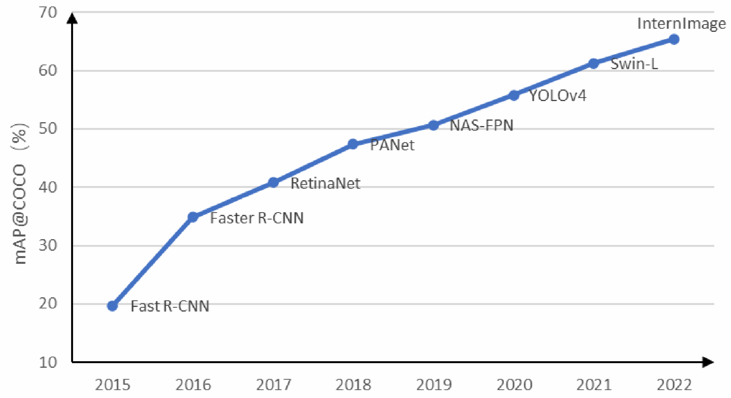Figure 1 shows the development of target recognition algorithms based on deep learning in recent years. New algorithms constantly set new records for the mean average precision (mAP) on the COCO dataset [5].

Deep learning is a subset of machine learning that involves computational structures with multiple layers of neural networks. A single-layer neural network can be viewed as a computational graph of the Credit Assignment Path (CAP), which outlines the potential causal relationships between data inputs and outputs. Research has demonstrated that a CAP with a depth of two can simulate any function [6]. Consequently, deep learning possesses more robust learning and representation capabilities than traditional shallow machine learning algorithms.

In recent times, deep learning has been gradually applied to practical engineering. Deep learning has become an important means of current target detection. Current object detection algorithms leveraging computer deep learning encompass two-stage detection methods such as R-CNN, Faster-CNN, Faster R-CNN, and FPN, as well as single-stage detection methods such as Over Feat, SSD, and the YOLO series [7,8,9,10,11]. The former mainly use the Select Search algorithm to extract target features and preselect boxes for mapping, then use Rol Pooling to pool feature maps of the same size, and finally perform classification and regression. However, omitting the results of the generation of preselected boxes often leads to a loss of detection accuracy [12,13,14,15].

We first introduce object detection algorithms based on two stages. Girshick et al. proposed RCNN, and the average accuracy was highly improved overall. Then, Girshick et al. [16] proposed the Fast-RCNN algorithm and directly added an image to the network for training so as to avoid the calculation redundancy caused by too many feature extraction boxes, which improved not only the detection speed but also the detection accuracy. Ren et al. [17] then proposed the Faster-RCNN algorithm, which uses the Region Proposal Network (RPN) to perform bounding box regression.

Next, we present object detection algorithms that operate on a one-stage basis. We focus on the YOLO algorithm. The YOLO algorithm for the detection of road cracks or other cracks has undergone rapid development. H. Yu [18] addressed the problems of missed detection. F. Yan [19] changed the residual unit to dense connection and increased the channel attention mechanism in the CSP module to improve the YOLO algorithm. The improved network alleviated the gradient disappearance problem and reduced the number of parameters. Wang, M. [20] proposed a multi-target intelligent recognition method (YOLO-T). Xu, H. [21] proposed the Cross-Stage Partial Dense YOLO (CSPD-YOLO) model, which is based on YOLO-v3 and the Cross-Stage Partial Network. It was proven to be more suitable for insulator detection. Venkat Anil Adibhatla [22] proposed a YOLOv5 algorithm with an attention mechanism to detect defects in PCB. Its efficiency, accuracy, and speed were found to be better than those of the traditional YOLO model. Hurtik, P. [23] proposed a model called poly-YOLO, which overcame some of the shortcomings of YOLOv3. Moran Ju [24] proposed an algorithm for the low detection rate of small targets, and, through a comparison of experimental results, it was found that the improved algorithm had a more obvious detection effect. X.Liu [25] explored YOLOv5 for the detection targets. Q. Chen [26] fused YOLOv3 and the SENet attention mechanism to complete the identification of missing spare nuts in a high-speed railway, and the recognition accuracy of the improved algorithm could reach 88.24%. Liu, C. [27] proposed the MTI-YOLO network. Zhang, Y. [28] employed the Flip Mosaic algorithm to augment the network’s detection of small targets. This improved YOLOv5 (Flip Mosaic) demonstrated improved accuracy and a reduction in the false detection rate.

From this, we can conclude that artificial methods are no longer used to identify cracks. At present, crack recognition based on computer vision and deep learning techniques is the mainstream. The YOLO series is widely used as a real-time monitoring algorithm, which can be applied not only in the field of building safety but also in fields such as marine life identification and smoke detection.

This study is mainly based on the following three points. By introducing the SIoU loss function, this study injects “directionality” into the model. The innovation of SIoU lies in its treatment of the direction alignment angle as one of the core elements in the loss calculation. When the direction of the predicted box aligns with that of the real box, the loss will significantly decrease; conversely, a penalty term proportional to the angle deviation will be imposed. This improvement fills the gap in general object detectors lacking geometric direction prior knowledge when dealing with slender targets. It forces the model to not merely “box” but to pursue “alignment”, enabling the output bounding boxes to fit the actual direction of the crack more closely and accurately. This is crucial for subsequent quantitative analysis of crack length, width, etc., and it is a key step from “detection” to “measurement”. The Mish activation function is used instead of ReLU. Mish is a smooth, non-monotonic function that allows small negative values to pass through and is smooth and differentiable throughout its domain. This fills the gap in traditional activation functions in capturing and transmitting low-contrast, blurred edge features. The smoothness of Mish helps the stable flow of gradients, alleviates the problem of gradient disappearance, and enables the network to more finely learn the hidden and faint crack features that are ignored by ReLU. This directly improves the model’s recall rate for early and subtle cracks in complex scenarios. The EfficientFormerV2 attention mechanism is integrated. This is a lightweight Transformer architecture specifically designed for visual tasks; it ingeniously combines the local feature extraction ability of convolution and the global dependency modeling ability of Transformer, and it significantly reduces computational complexity through structural optimization. This fills the “performance efficiency” gap between lightweight CNNs and heavyweight Transformers. It makes it possible to introduce powerful attention functions similar to those of Transformers while maintaining the high inference speed (operability) of YOLOv5. The model can dynamically focus on the crack area; suppress background noise; and find a better balance between accuracy and speed, which is especially suitable for practical applications with real-time requirements.

This study introduces an advanced YOLOv5 framework for the identification of road cracks, capitalizing on the algorithm’s proven dependability in object detection. The study emphasizes three key enhancements: structural optimizations aimed at reducing computational complexity via a streamlined network architecture, enhanced attention modules designed to improve feature discrimination in crack pattern analysis, and the adoption of innovative loss computation techniques coupled with sophisticated activation functions to enhance detection accuracy. Experimental results confirm the optimized algorithm’s operational efficiency, revealing significant advancements in performance metrics such as precision and inference speed when compared to current detection systems.

2. Methods

2.1. Overview of the YOLOv5 Algorithm

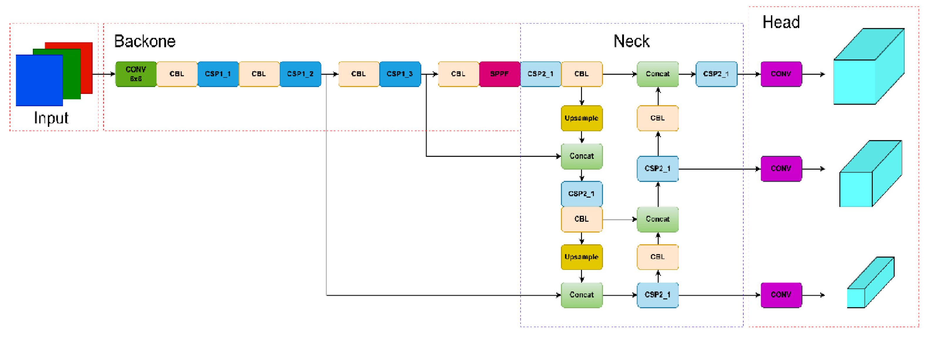
The YOLOv5 algorithm primarily consists of three components: a feature extraction backbone network, a feature fusion neck network, and a detection head. The backbone network is composed of a convolution module (Conv), C3 module, and spatial pyramid pooling module (SPPF), which is used to extract the main features at different scales. The neck network follows the structure of FPN+PAN, which is used to further strengthen the fusion features and realize multi-scale divide-and-conquer detection. The network structure is shown in Figure 2.

The detection process is generally segmented into three stages. Initially, feature extraction is performed. Subsequently, feature fusion takes place. Finally, the prediction of the target’s type and location is executed. The input of YOLOv5 mainly consists of three parts: mosaic data enhancement, adaptive anchor box calculation, and adaptive image scaling. Mosaic data enhancement stitches four images into a picture via random cropping and random scaling, which indirectly increases the number of dataset samples and enhances the detection ability for small objects. In YOLOv3, the K-means algorithm is used to obtain the preset anchor box suitable for each dataset, while YOLOv5 compares and calculates the real box on the basis of the preset anchor box and then updates it in the reverse direction. In common detection algorithms, image scaling is used to uniformly scale the original images to the same scale. Adaptive image scaling makes the ratio of the image’s length and width the same, which effectively reduces the number of calculations.

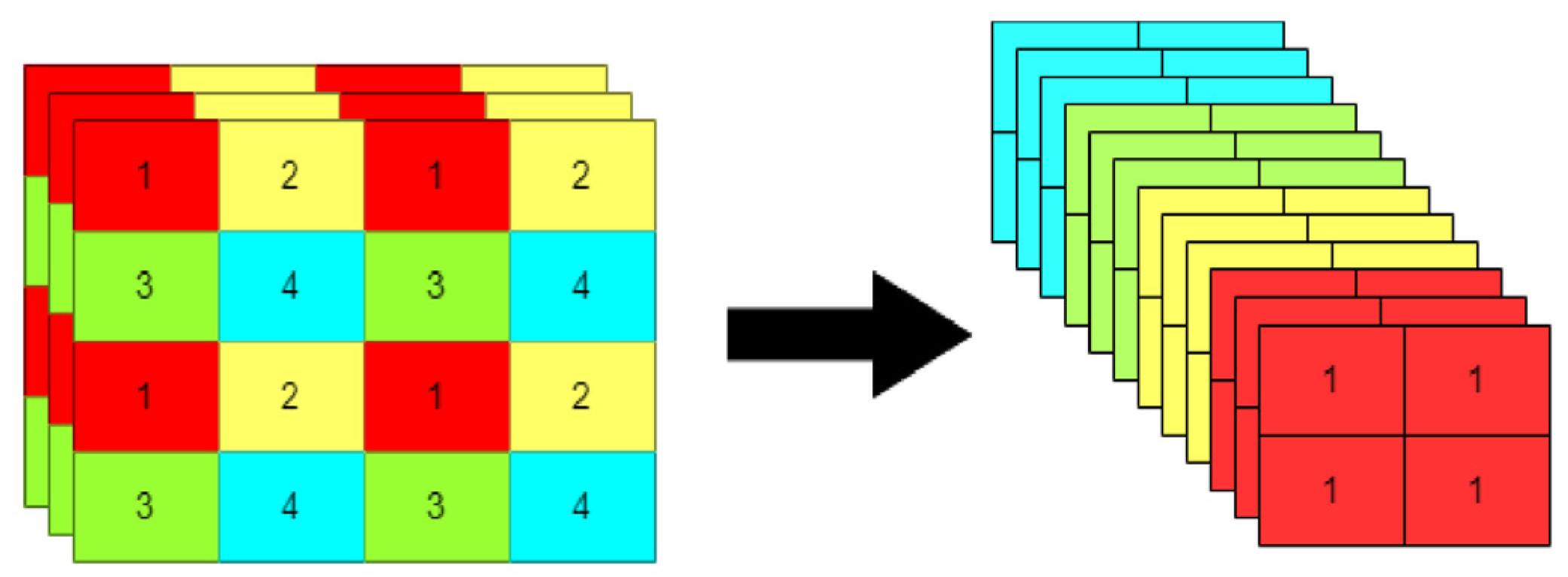
Backbone mainly consists of a 6 × 6 convolution layer, CSP, and SPPF three-part structure. In the v6.0 version, YOLOv5 uses a 6 × 6 size convolution layer to replace the Focus structure. The Focus structure is used to convolve four new images obtained by splicing after slicing in the image, as shown in Figure 3. This operation does not cause information loss and improves the detection speed. Using a 6 × 6 size convolution layer is theoretically equivalent to using the Focus structure, but existing devices use 6 × 6 convolution layers more efficiently than the Focus structure.

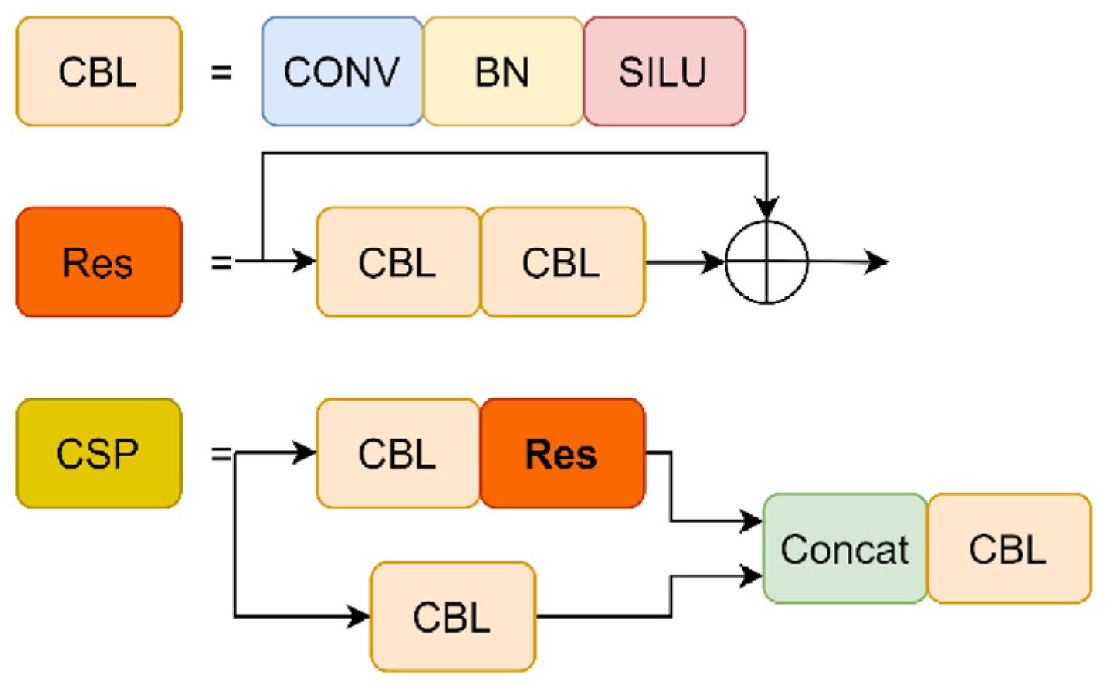
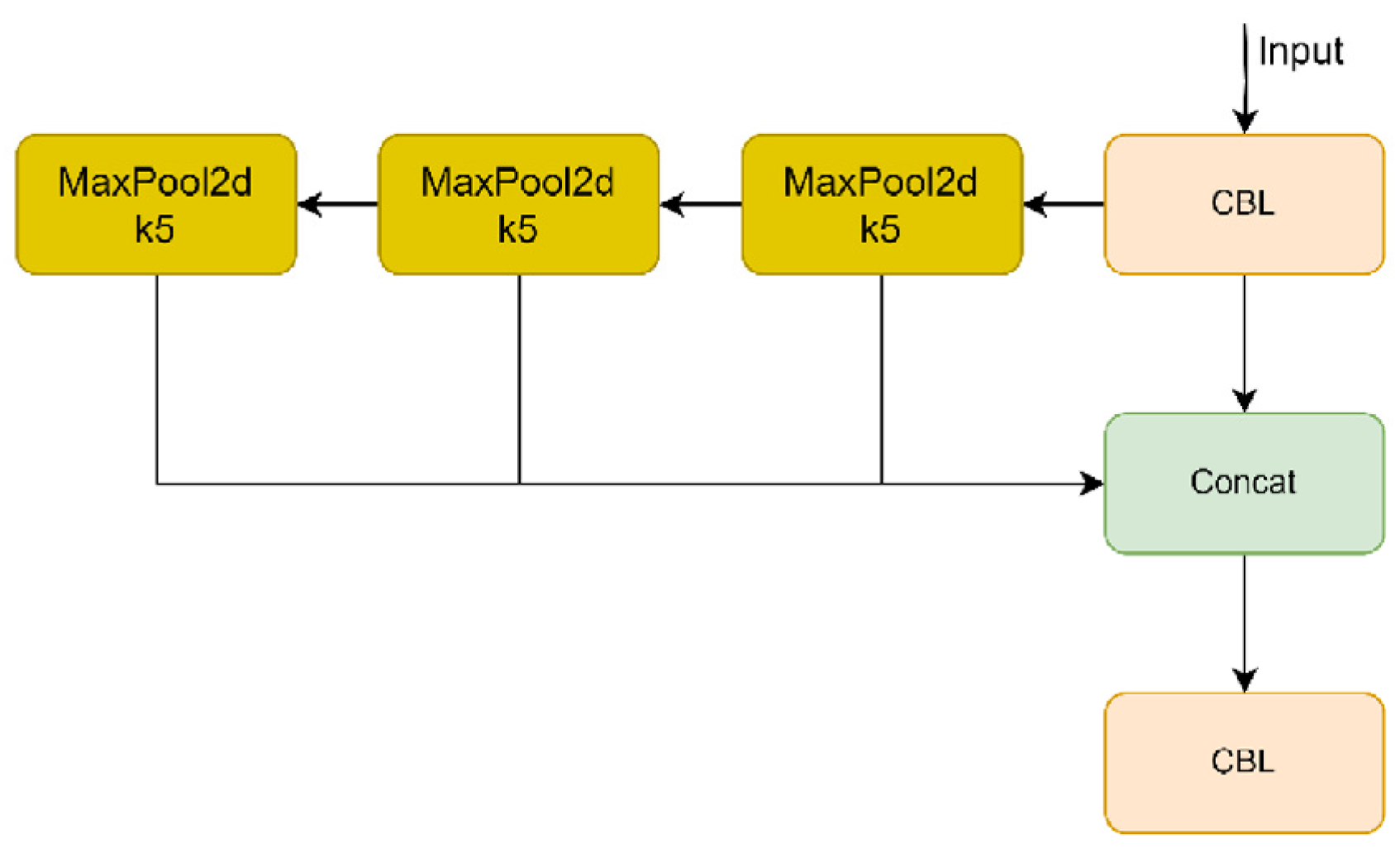
Although DarkNet-53 has good accuracy in image classification, it relies too much on computing resources. YOLOv5 adds a CSP structure to DarkNet-53 [29] and divides the feature map into tiles for YOLOv5; backbone uses CSP1_X with a residual structure, as shown in Figure 4; and neck uses CSP2_X without a residual structure. In the v6.0 version, YOLOv5 uses an SPPF structure to replace the SPP structure. The SPP structure uses three different convolution kernel sizes, and two parts are passed through the base layer, one part is output by the convolution block, and the other parts are combined. The number of parameters and memory usage are reduced. There are two CSP structures with 5 × 5, 9 × 9, and 13 × 13 convolutions in parallel for max-pooling operations and concatenation with the previous layer, which improves the diversity of image size and makes the network easier to converge. The SPPF structure serially uses three 5 × 5 convolution kernels to perform the max-pooling operation, as shown in Figure 5. The calculation results of both structures are the same, but SPPF uses a smaller convolution kernel, so its calculation speed is two times faster than that of SPP.

Neck consists of FPN [30] and PAN [31]. FPN is a pyramid structure with up-sampling fusion from top to bottom, which transmits high-level semantic information and enhances semantic expression at multiple scales, but the positioning information is weak. PAN is a pyramid structure with down-sampling fusion from bottom to top, which transmits strong positioning information at the low level to enhance the positioning ability at multiple scales. The combination of the two makes the network obtain richer feature information. Each detection layer detects the corresponding object type, object confidence, and object bounding box. The binary cross-entropy loss function is applied to determine classification and confidence losses, whereas the CIoU function is used to compute the bounding box loss.

2.2. New Loss Function SIoU

The design of error metrics plays a critical role in the performance of object detection frameworks, serving as a fundamental component in modern detection algorithms. During model optimization, this error metric needs to be progressively minimized through iterative adjustments, ideally achieving precise alignment between predicted bounding areas and their corresponding ground-truth annotations. Contemporary implementations in YOLOv5 variants employ a combination of localization evaluation parameters, such as GIoU and CIoU, which incorporate spatial relationships, including centroid displacement, overlapping regions, and dimensional proportions. However, current methodologies neglect directional discrepancies between predicted and actual bounding coordinates, potentially causing suboptimal gradient updates during backpropagation. This oversight may lead to oscillating parameter adjustments during neural network training, ultimately prolonging convergence periods and compromising final model accuracy.

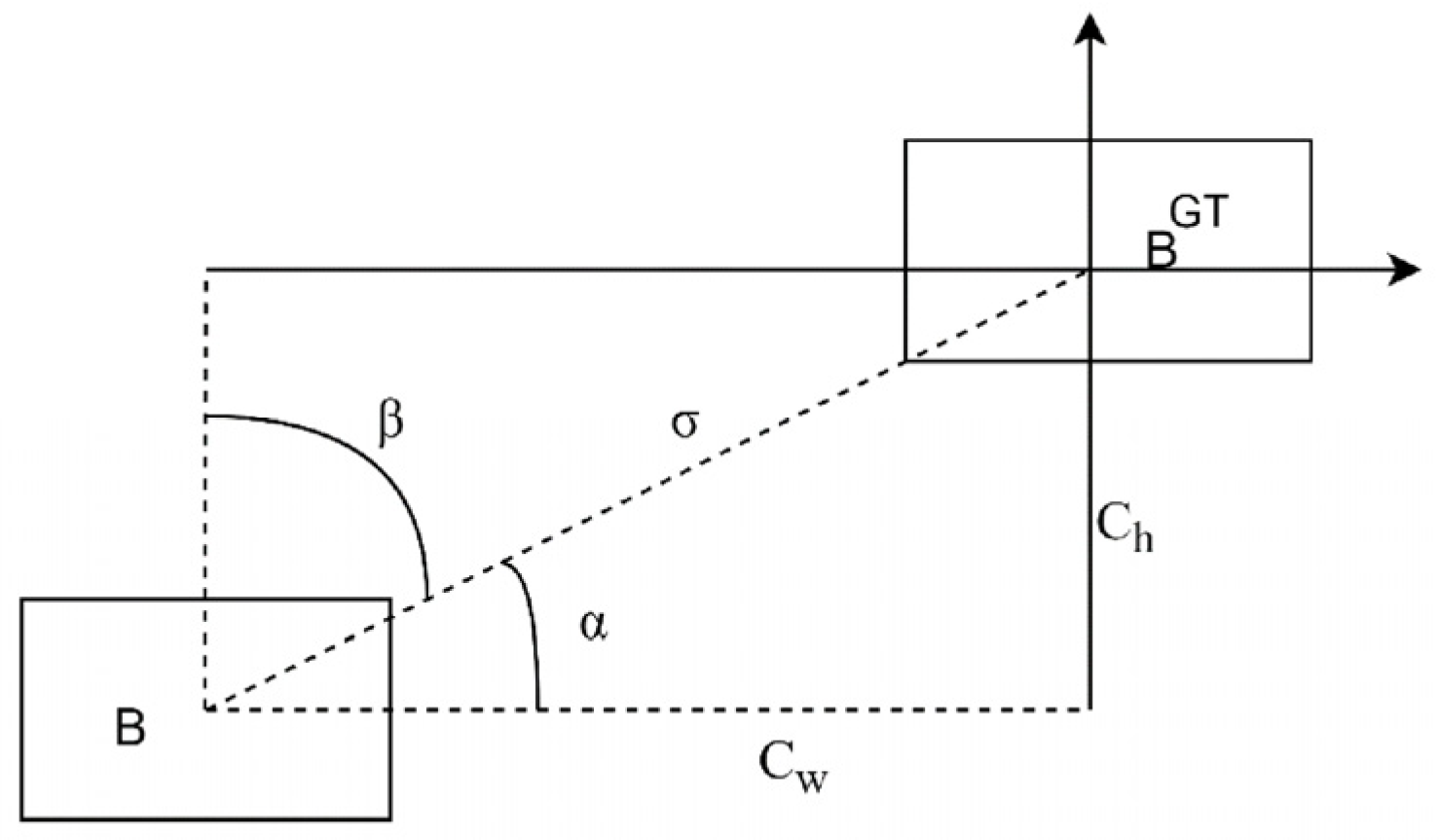
This study proposes an innovative loss function, referred to as SIoU [32], which modifies conventional penalty metrics and incorporates angular vector considerations into the regression framework, as depicted in Figure 6. The architectural refinement significantly enhances model training efficiency by accelerating parameter convergence, particularly through optimized directional learning, which guides bounding boxes toward target coordinates with reduced positional deviation. This geometric constraint mechanism effectively minimizes the oscillatory behavior of bounding box predictions during optimization phases. The proposed methodology is successfully implemented with the YOLOv5 architecture, demonstrating measurable improvements in both training dynamics and detection precision across experimental evaluations.

For SIoU to increase angle perception, part of the loss function minimizes the variables related to distance. Specifically, as shown in Equation (1), the method first moves the prediction attempts close to the X or Y axis and then continues making predictions along the relevant axes. To accomplish this objective, in the convergence process, if $\alpha \le {\displaystyle \frac{\pi }{4}}$, minimize the first taste $\alpha$; otherwise, minimize $\beta ={\displaystyle \frac{\pi }{2}}-\alpha$.

$$\mathrm{\Lambda }=1-2\times {\sin }^2(\arcsin (x)-{\displaystyle \frac{\pi }{4}})$$

(1)

$$x={\displaystyle \frac{c_h}{\sigma }}=\sin (\alpha )$$

(2)

$$\sigma =\sqrt{(b_{cx}^{gt}-b_{cx}{)}^2+{(b_{cy}^{gt}-b_{cy})}^2}$$

(3)

$$c_h=\max (b_{cy}^{gt}-b_{cy})-\min (b_{cy}^{gt}-b_{cy})$$

(4)

$\sigma$ represents the distance separating the center point of the actual box from that of the estimated box; $c_h$ denotes the variation in height between the center point of the actual box and that of the estimated box; $b_{cx}^{gt}$ and $b_{cy}^{gt}$ are the real box center point coordinates; and $b_{cx}$ and $b_{cy}$ are the center point coordinates of the prediction box. Because the angle loss is added, the distance loss is redefined.

$$\mathrm{\Delta }={\mathrm{\Sigma }}_{t=x,y}(1-e^{-\gamma \rho t})$$

(5)

$${\rho }_x={({\displaystyle \frac{b_{cx}^{gt}-b_{cx}}{c_w}})}^2,{\rho }_y={({\displaystyle \frac{b_{cy}^{gt}-b_{cy}}{c_h}})}^2,\gamma =2-\mathrm{\Lambda }$$

(6)

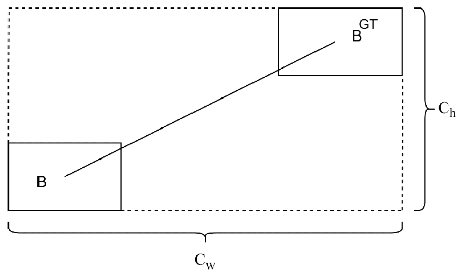
$c_w,c_y$ are the dimensions, specifically the width and height of the smallest bounding rectangle that encompasses both the actual and forecasted boxes, as shown in Figure 7. It can be seen from the above that, when $\alpha \to 0$, it will revert to the normal distance loss calculation, and bounding box regression will become more difficult as the angle increases.

The shape loss is defined using the following formula:

$$\mathrm{\Omega }={{\displaystyle \sum _{t=w,h}(1-e^{-w_t})}}^{\theta }$$

(7)

$${\omega }_w={\displaystyle \frac{\left|w-w^y\right|}{\max (w,w^{gt})}},{\omega }_h={\displaystyle \frac{\left|h-h^y\right|}{\max (h,h^{gt})}}$$

(8)

$w,h,w^{gt},h^{gt}$ predict the box and real frame’s width and height, respectively. $\theta$ defines how much the shape loss should be. The value of $\theta$ is unique to each dataset, and it controls how much attention is given to the shape loss. If $\theta$ is set to 1, it will immediately optimize the shape, thus affecting the free movement of the shape. $\theta$ typically ranges from 2 to 6. Finally, the loss function is defined in the following formula:

$$L_{box}=1-IoU+{\displaystyle \frac{\mathrm{\Delta }+\mathrm{\Omega }}{2}},IoU={\displaystyle \frac{B\cap B^{gt}}{B\cup B^{gt}}}$$

(9)

Imagine that a prediction box is located to the upper right of the real box. Traditional loss functions (such as IoU, GIoU, and CIoU) would calculate both the center point distance and the width and height differences simultaneously and give equal optimization weights. This means that the model might try to move both left and down at the same time or adjust the width and height first and then move the position. This optimization path is ambiguous and oscillatory, similar to someone feeling their way towards a goal in the dark, possibly swaying left and right. SIoU gives a “direction sense” to the regression process by defining angle costs. It achieves this through the following geometric steps: Step 1: Define vectors and angles. Step 2: Measure the deviation of the direction. Step 3: Integrate the angle cost into the total loss. We can compare this process to docking a ship:

Traditional loss function (CIoU): The captain simultaneously orders all engines and lateral thrusters to operate at full power, attempting to directly approach the berth. This causes the ship to violently sway in front of the berth, constantly making excessive corrections. Although it manages to dock eventually, the path is crooked and time-consuming (slow convergence and unstable).

SIoU Loss Function: An experienced captain first takes a crucial action—“aligning the ship’s hull”. He first operates the vessel to make its axis parallel to the axis of the berth (this corresponds to the angle priority strategy in SIoU). Once the hull is aligned, he only needs to simply control the front and rear engines and make minor lateral shifts to smoothly enter the berth (this corresponds to the subsequent fine-tuning of position and size). The angle consideration in SIoU essentially introduces a geometric prior-based optimization strategy into the bounding box regression problem. It transforms an unordered, multi-variable optimization problem into an ordered, phased process:

Phase 1: Orientation Calibration—By using the angle cost, prioritize aligning the axial direction of the predicted box with that of the actual box.

Phase Two: Fine-tuning of Position and Shape—Based on the correct direction, further refine the position of the center point and the width and height dimensions.

This “first orientation, then fine-tuning” mechanism mimics the cognitive process of humans when performing precise positioning tasks, thereby fundamentally solving the problem of unclear regression paths in traditional methods and significantly improving the stability, speed, and final accuracy of bounding box regression.

2.3. New Activation Function Mish

Action functions play an important role in learning complex or nonlinear functions. The activation function can often be a weighted sum of linear models, resulting in it having more complex nonlinear neurons instead of ordinary matrix multiplication. The Relu activation function is used in the YOLOv5 algorithm. The Relu activation function has good sparsity and simple calculation, and it is the most widely used unsaturated nonlinear activation function in convolutional neural networks. Its formula is as follows:

$$\mathrm{Re}lU(x)=\max (0,x)$$

(10)

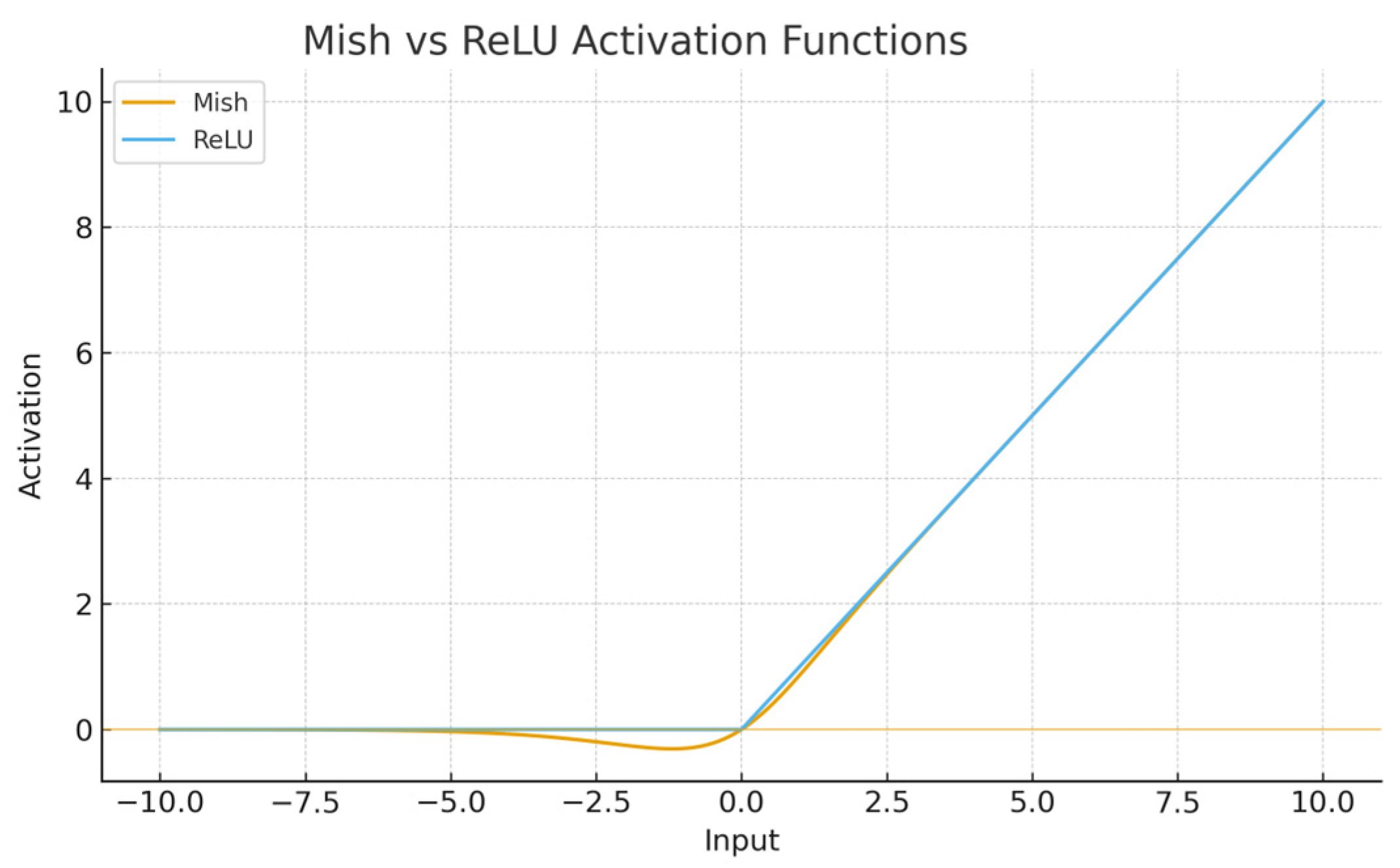
When $x>0$, there are no problems such as vanishing gradients or gradient unsaturation; when $x<0$, the neuron gradient is 0, and forward propagation is no longer carried out, so the model cannot be updated, and the training effect is not ideal. Figure 8 shows that the Mish activation function has no upper boundary, which can effectively suppress the gradient saturation phenomenon. For negative values, it has a more stable gradient flow, and the gradient disappearance problem will not occur during training. The gradient of the Mish activation function is smoother than that of the Relu activation function. It can stably transfer information to deep networks, so it has better accuracy and generalization power. The formula for the Mish activation function is given in the following equation:

$$Mish(x)=x\times \tanh (\ln (1+e^x))$$

(11)

where $x$ represents the input value $x_i=[x_1,x_2,\dots ,x_n]$, and $\tanh$ denotes the hyperbolic tangent function.

2.4. Backbone Network Combined with New Attention Mechanism

The attention mechanism serves as a data processing technique that has gained extensive application across multiple deep learning domains over the past few years, encompassing areas such as image processing, speech recognition, and natural language processing. The attention mechanism originates from a signal processing mechanism in human vision, and humans naturally pay attention to objects in a scene. For example, when observing a new scene, the human visual system does not process the whole visual scene at once but quickly allocates attention to the important regions for a concentrated analysis while ignoring some of the unimportant regions, so as to be able to identify the most relevant information. The essence of the attention mechanism is equivalent to learning a weight distribution and then reweighting the input image features, giving high weights to important features, strengthening the accumulation of significant attributes within the feature map, and reducing the weight of unimportant features, thereby losing some redundant information.

An attention mechanism is incorporated into the backbone network of YOLOv5. The role of this mechanism is to make the algorithm pay more attention to important features in the image while ignoring less important information. This attention mechanism is usually achieved by calculating weights. These weights indicate the importance of different parts in image processing. SENet, CBAM, and CA are three traditional attention mechanisms. In this study, we adopt a new attention mechanism: EfficientFormerv2. After adding the new attention mechanism, the YOLOv5 algorithm can process the image more effectively and complete the detection task in a shorter time.

2.4.1. SENet

Hu et al. [33] pioneered the development of channel-wise attention mechanisms through their SENet architecture, which achieved top performance in the ImageNet2017 competition. This innovative framework employs a squeeze–excitation (SE) block comprising two distinct operational phases. The system initially captures comprehensive spatial data through feature compression and then dynamically prioritizes critical feature channels through an inter-channel relationship analysis.

The SE mechanism operates through sequential processing stages: spatial feature aggregation, followed by adaptive channel recalibration. Through global average pooling operations, the squeeze component condenses spatial features across each channel to establish global context. Subsequently, the excitation unit employs a gating mechanism with fully connected layers and sigmoid activation to model channel interdependencies, generating channel-specific scaling factors. These learned parameters are then applied to the initial feature maps through element-wise multiplication, effectively enhancing discriminative feature representations while suppressing less relevant channels.

The recalibration mechanism enables targeted feature enhancement through adaptive scaling, producing attention-augmented feature representations. SENet constitutes a versatile and efficient attention architecture, characterized by its straightforward design and seamless integration into existing models. This approach amplifies the model’s focus on critical channel characteristics while diminishing the influence of less relevant features.

2.4.2. CBAM

In 2018, Woo et al. [34] introduced the Convolutional Block Attention Module (CBAM) to optimize the effectiveness of convolutional operations through integrated spatial and channel-wise attention mechanisms. This architecture sequentially processes features through channel- and spatial-focused attention submodules, with refined feature maps obtained through element-wise multiplication with the original input features. The channel attention mechanism employs dual-path feature condensation using global maximum and average pooling operations across spatial dimensions, followed by parallel processing through multi-layer perceptrons. These processed features are subsequently merged and normalized via activation functions to generate channel-specific attention coefficients, which are then combined via multiplicative operations to produce refined features for spatial attention processing. The spatial attention component further processes these features by applying cross-channel pooling operations, aggregating the maximum and average values across channel dimensions to construct spatial attention maps that highlight significant regions within the feature space.

The convolution operation processes the input data, with spatial attention coefficients derived through an activation function. This computational stage generates attention-enhanced features via element-wise multiplication between module inputs and calculated weights. The mechanism compensates for potential information loss in channel attention by capturing spatially significant patterns, enabling complementary interaction when both modules operate concurrently. As a versatile lightweight architecture, the CBAM effectively amplifies critical channels while intensifying feature-rich spatial regions through its dual-attention mechanism.

2.4.3. CA

SENet processes spatial features through global max-pooling operations but does not account for positional significance. While the CBAM applies convolutional operations to detect proximate spatial correlations after channel reduction, this approach fails to establish interconnections across extended spatial ranges. Addressing these limitations, Hou et al. [35] developed Coordinate Attention (CA), which integrates channel-wise and spatial data while embedding positional cues within attention mechanisms, enabling efficient identification of critical feature areas. This mechanism operates through two distinct phases: coordinate-based feature encoding and attention map formulation. Unlike conventional methods employing global averaging, CA implements directional feature compression. The encoding stage utilizes axis-specific pooling operations to create orientation-aware channel descriptors, separately capturing horizontal and vertical spatial patterns through dedicated pooling pathways.

The network produces dual-embedded feature maps containing both long-range contextual relationships and exact spatial coordinates. The coordinate generation mechanism combines these representations through sequential processing: initial 1 × 1 convolutional operations transform and spatially partition the tensor into complementary components. Subsequent channel alignment via 1 × 1 convolutions matches input dimensions before nonlinear activations yield axis-specific attention coefficients. These directional weights subsequently refine the input features through element-wise modulation. Designed as a computationally efficient architecture, the Coordinate Attention (CA) mechanism adapts seamlessly to diverse deep learning frameworks while strengthening feature discriminability. Unlike the CBAM’s approach, CA achieves superior performance through an expanded perceptual scope and enhanced spatial reasoning capabilities for target localization.

2.4.4. EfficientFormerV2

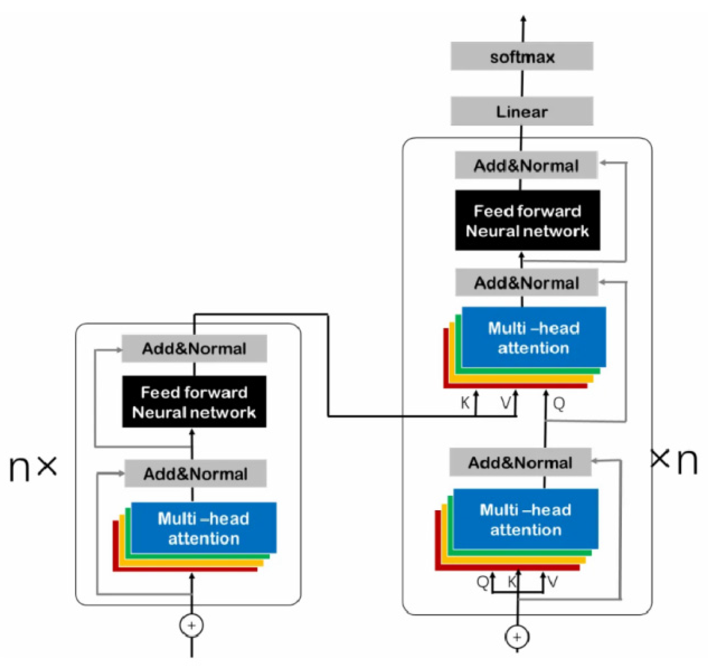
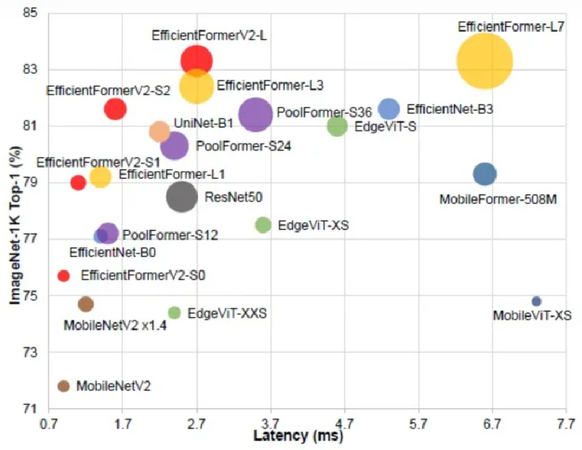
A transformer is a neural network structure based entirely on an attention mechanism. It plays an important role in SE and the CBAM. SE and the CBAM are often used to compute channel and spatial dimension attention; this attention actually refers to the importance of features and is obtained implicitly through convolution or fully connected layers. Vision Transformers (ViTs) [36] have made rapid progress in computer vision tasks, prompting the Vision + Transformer initiative, and a large number of papers and studies have been based on ViTs. However, Transformers perform a bit slower than specially optimized CNNs due to the large number of parameters required by the attention architecture. Therefore, based on the above considerations, a lightweight network structure should be developed while ensuring accuracy. After performing a series of design and optimization steps on Mobile Net, an efficient network with low latency and size, EfficientFormerV2, is developed. Figure 9 shows an accuracy comparison plot.

Transformer Network Architecture

Based on an attention mechanism, Transformer represents a neural network framework [37], and its comprehensive structural details are shown in Figure 10. This architecture has gained significant research attention due to its versatile applications across natural language processing and computer vision domains.

Transformers’ network structure primarily consists of an encoder and a decoder. The encoder processes the input sequence, while the decoder decodes the processed sequence to produce the final output. The primary architecture of the Transformer network consists of the following:

Input embedding layer: Each element of the input sequence (such as words or pixels in an image) is converted into a vector representation for subsequent processing.

Position encoding layer: Position encoding is added to each element in the input sequence to retain the position relationship information of the element in the sequence.

Multi-head self-attention layer: The multi-head self-attention mechanism is used. That is, each element in the input sequence is regarded as a query, key, and value; the attention weight of each element is obtained by calculating the similarity between them; and then these weighted values are weighted and operated to obtain the encoded sequence representation.

Feedforward fully connected layer: The feedforward fully connected operation is performed on the encoded sequence representation to improve the nonlinear modeling ability of the model.

Encoder layer: This layer consists of multiple multi-head self-attention layers and feedforward fully connected layers, which are used to perform multiple encoding operations on the input sequence so as to obtain a more comprehensive and accurate sequence representation.

Decoder layer: Composed of multiple multi-head self-attention layers, multi-head attention layers, and feedforward fully connected layers, this layer is used to decode the encoded sequence to obtain the final output. Transformers have achieved good results in several natural language processing and computer vision tasks, and it has become one of the most advanced neural network architectures.

Transformer Core Components

Transformers have three core components, each of which we describe next.

The first core component is self-attention. The self-attention layer is the core of the whole network. Its main role is to consider each element in the input sequence (such as words or pixels in an image) as a query, key, and value; obtain the attention weight of each element by calculating the similarity between them; and then perform a weighted sum operation on these weighted values to obtain the encoded sequence representation. The formula is as follows:

$$FFN(x)=\max (0,x{W}_1+b_1)W_2+b_2$$

$$\begin{array}{c}Q=X{W}_Q\\ K=X{W}_K\\ V=X{W}_V\\ Attention(Q,K,V)=Soft\max ({\displaystyle \frac{Q{K}^T}{\sqrt{d_k}}})V\end{array}$$

(12)

The second core component is masked attention. In Transformers, an important difference between the encoder and decoder is that the input layer of each unit of the decoder first goes through a masked attention layer. The encoder needs to encode the entire sentence, so each word takes into account the information of all other words in the context. However, the decoder is similar to the decoder in the Seq2Seq model, where each word can only see the state of the previous word, so the decoder only employs one-way self-attention. To achieve this one-way self-attention, the decoder needs to perform masked attention before performing the self-attention calculation; that is, before the normal self-attention Softmax calculation, the weight matrix is AND-operated with a lower triangular matrix M to mask the information of words after the current position. In this way, the decoder can only see the state of the word that precedes each current word, thus achieving one-way self-attention. The formula is as follows:

$$Attention(Q,K,V)=Soft\max ({\displaystyle \frac{Q{K}^T\mathrm{\Theta }M}{\sqrt{d_k}}})V$$

(13)

The third core component is a position-wise feedforward network. This is an important component in Transformer. Its main role is to perform a nonlinear mapping of the vector of each sequence position so as to enhance the model’s representational ability. Specifically, position-wise feedforward networks are composed of two fully connected layers. Position-wise feedforward networks have the advantage that the computation can be performed very quickly for each position in the sequence, as the computation between them is independent and can be parallelized. At the same time, they introduce nonlinear transformation, so they can capture more complex sequence relationships and improve the representation ability of the model. The formula is as follows:

$$FFN(x)=\max (0,x{W}_1+b_1)W_2+b_2$$

(14)

Backbone Network Structure Optimization

After identifying the backbone based on the Transformer architecture, it is important to note that this architecture still has some limitations in the object detection domain. Specifically, this leads to more complex challenges due to the large differences in the scale of the targets. Unlike the NLP domain, object sizes in object detection are not fixed. In addition, the Transformer architecture is relatively complex and requires higher hardware resources, and its performance cannot be fully utilized if the hardware conditions are poor.

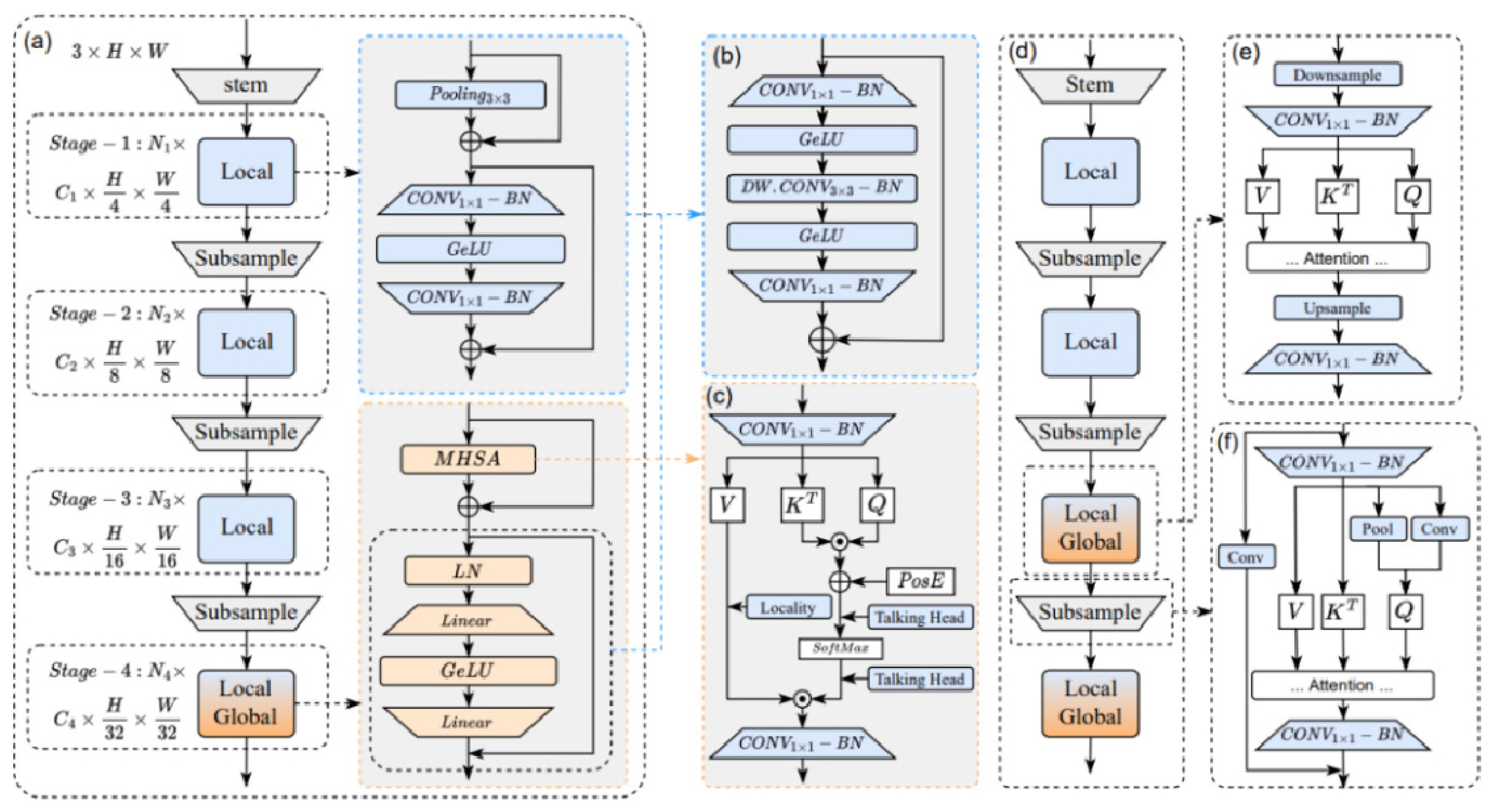
Considering the ongoing research and development, EfficientFormerv2 [38] was built based on an efficient Transformer architecture. The configuration is depicted in Figure 11, where (a) shows the EfficientFormer network as the baseline model, (b) shows the uniform FFN, (c) shows the MHSA improvement, (d) and (e) note the higher resolution, and (f) shows the down-sampling process. Based on the original Transformer, the model has been refined and enhanced to boost its performance and efficiency.

An analysis of ViT’s foundational architecture reveals that integrating local structural information enhances model efficacy while boosting stability when positional encoding is unavailable. As illustrated in Figure 11a, both PoolFormer and EfficientFormer [39] employ 3 × 3 average pooling operations as localized token integration mechanisms, subsequently substituting these with depth-wise convolutional layers matching kernel dimensions without increasing temporal overhead. Implementing localized feature modeling within ViTs’ feedforward networks (FFNs) presents a cost-effective strategy for performance enhancement, combining computational efficiency with improved operational outcomes through spatial-aware processing layers. This approach demonstrates that the strategic insertion of regional data analysis components significantly optimizes network functionality while maintaining computational efficiency.

To enhance computational efficiency, EfficientFormerv2 introduces a bottleneck architecture that replaces the conventional pooling layer, as illustrated in Figure 11b. This architectural modification sequentially applies 1 × 1 convolutional layers for channel reduction, followed by 3 × 3 depth-wise separable convolutional layers for spatial feature extraction, concluding with 1 × 1 convolutions for dimensional expansion. The redesigned module enables automated network depth optimization through hyperparameter search algorithms while effectively capturing both localized and contextual patterns, thereby expanding the model’s theoretical receptive field and strengthening system resilience. Furthermore, this structural innovation offers the dual advantages of enhanced operational effectiveness and configurable network depth parameters.

Transformer architectures typically comprise two fundamental components: a multi-head self-attention (MHSA) mechanism and a feedforward network (FFN). Through a comprehensive analysis of various MHSA implementations, we develop enhancement strategies that boost attention module effectiveness while maintaining computational efficiency. Our first innovation integrates localized feature extraction by applying depth-wise 3 × 3 convolutional operations to the value matrix, as visualized in Figure 11c. This spatial-aware modification complements the existing attention mechanism with position-sensitive processing. Additionally, we strengthen inter-head communication through a novel cross-head interaction mechanism implemented via a specialized feedforward layer operating along the head dimension, enabling dynamic information exchange between attention heads without parameter inflation.

An attention mechanism is commonly used to improve performance, and it makes inference and selection on a global basis.

However, when applied to high-resolution images, features lead to less efficient end-to-side inference because the time complexity scales squarely with the spatial resolution. To address this, EfficientFormerv2 uses a novel MHSA method that applies the attention mechanism at the last 1/32 spatial resolution and uses it at the penultimate stage, which is 4x down-sampling. In addition, EfficientFormerv2 also performs MHSA at an early stage of the network by down-sampling all queries, keys, and values to a fixed spatial resolution of 1/32, and then it reverts the attention output to its original resolution to feed it into the next layer in order to improve the inference efficiency, as shown in Figure 11d,e.

$$Ou{t}_{\left[B,H,N,C\right]}=(Q_{\left[B,H,NC\right]}\cdot {K^T}_{\left[B,H,C,\frac{N}{2}\right]})\cdot V_{\left[B,H,\frac{N}{2},C\right]}$$

(15)

Here, Out is the output resolution after the multiplication of attention matrices; Q is the full-resolution query; K and V are the down-sampled key value pairs; and B, H, N, and C represent the batch size, number of heads, number of tokens, and channel dimensions, respectively.

EfficientFormerv2 proposes a composition strategy that combines local and global context fusion, as shown in Figure 11f. In this strategy, two down-sampling modes are used, one is the pooling layer as static local down-sampling, and the other is 3 × 3 DWCONV as learnable local down-sampling. The results of these two types of down-sampling are concatenated and projected into the query matrix to obtain the down-sampled query. In addition, to obtain a local–global form, the attention down-sampling module employs residual connections and is connected to a convolution layer with step size.

It is worth noting that, in order to further improve accuracy, EfficientFormerv2 also improves the attention down-sampling module. Specifically, by slightly increasing the parameter and time overhead, we introduce global down-sampling to increase the receptive field of the model and use a multi-branch attention down-sampling module to enhance the fusion of the local and global context. Taken together, this combined strategy, fusing the local and global context and improving the attention down-sampling module, significantly improves the accuracy of the model. The number of tokens in the query is halved so that the output of the attention module is down-sampled as shown in Equation (16):

$$Ou{t}_{\left[B,H,\frac{N}{2},C\right]}=(Q_{\left[B,H,\frac{N}{2},C\right]}\cdot {K^T}_{\left[B,H,C,N\right]})\cdot V_{\left[B,H,N,C\right]}$$

(16)

The search space of EfficientFormerV2 includes the depth and width of the network, as well as the spread ratio of each FFN. In order to build the search space, a slimmable network is used to achieve elastic depth and switchable width, and MHSA and an FFN are used as the basic modules of EfficientFormerV2. The Mobile Efficiency Score (MES) is a metric defined by EfficientFormerV2, as shown in Equation (17). To evaluate the performance of the visual backbone network on mobile devices, the MES is calculated by considering both model size and latency:

$$MES=Score\cdot {{\displaystyle \prod _i(\frac{M_i}{U_i})}}^{-a_i}$$

(17)

$a_i\left(0,1\right],M_i$ denotes the index value; $U_i$ denotes the unit of the indicator value; and $Score$ is a predefined base score, the initial value of which is set to 100.

In the search space, EfficientFormerV2 uses a pure search algorithm based on evaluation to search for the subnetwork with the best Pareto curve by analyzing the efficiency gain and accuracy drop of each reduction operation. Specifically, EfficientFormerV2 defines an action pool consisting of per-block width reduction and per-block depth reduction, and blocks are deleted from the action pool. Through these operations, the algorithm can find the subnetwork in the search space that has the optimal Pareto curve.

To further improve the performance of EfficientFormerV2, several post-processing techniques are employed, such as model distillation and model adaptive inference. These techniques can greatly reduce the model size and inference time while maintaining high accuracy and robustness.

Model Design for EfficientFormerv2

EficientFormerV2 is a lightweight transformer-based model that enables high-quality visual classification and object detection tasks to be performed on low-performance devices. The design process of this model mainly involves the following aspects:

EficientFormerV2 uses a four-stage hierarchical design, which obtains feature sizes of 1/4, 1/8, 1/16, and 1/32 of the input resolution. Instead of using inefficiently embedded non-overlapping patches, we start with a small kernel convolution stem to embed the input image. The formula is as follows:

$${\mathrm{X}}_{{i|}_{i=1,}{j|}_{j=1}}^{B,C_{{j|}_{j=1}},\frac{H}{4},\frac{W}{4}}=stem({\mathrm{X}}_0^{B,3,H,W})$$

(18)

$B$ denotes the batch size, $C$ denotes the width of the network, $H$ and $W$ refer to the height and width of the features, ${\mathrm{X}}_j$ is the feature in stage $j$, $j\in \left\{1,2,3,4\right\}$, and $i$ denotes the $i$-th layer.

The first two stages capture high-resolution local information, and EficientFormerV2 uses a unified FFN that is commonly described as follows:

$${\mathrm{X}}_{i+1,j}^{B,C_j,\frac{H}{2^{j+1}},\frac{W}{2^{j+1}}}=S_{i,j}\cdot FF{N}^{C_J,E_{i,j}}({\mathrm{X}}_{i,j})$$

(19)

$S_{i,j}$ represents a learnable level [40]. The FFN is composed of two attributes: stage width $C_j$ and expansion rate per block $E_i$.

In the last two stages, both local FFN and global MHSA blocks are used; thus, on the basis of common Equations (18), the global blocks are defined as

$${\mathrm{X}}_{i+1,j}^{B,C_j,\frac{H}{2^{j+1}},\frac{W}{2^{j+1}}}=S_{i,j}\cdot MHSA(\mathrm{Pr}oj({\mathrm{X}}_{i,j}))+{\mathrm{X}}_{i,j}$$

(20)

The query (Q), key (K), and value (V) are mapped from the input features through linear layers, and Q, K, V, MHSA is denoted by expression (21):

$$MHSA(Q,K,V)=Soft\max (Q\cdot K^T+ab)\cdot V$$

(21)

where ab is a learnable attention bias for positional encoding.

3. Results

3.1. Training Environment and Evaluation Metrics

This study uses publicly available datasets and self-collected data as data sources, aiming to cover various pavement materials, lighting conditions, and weather conditions, thereby ensuring the richness of the scenarios. All images are finely annotated using bounding boxes and are classified into multiple categories such as longitudinal and transverse based on the crack morphology. To ensure the rigor of model evaluation and generalization ability, we first conducted a systematic bias analysis on the dataset to identify potential issues such as class imbalance and uneven scene distribution. In response to these biases, we comprehensively employed data augmentation techniques, including color jittering and geometric transformation, and combined weighted loss functions for algorithmic compensation to alleviate the impact of data imbalance on model training. Through the above data construction and bias correction strategies, we aimed to build a high-quality and highly robust benchmark dataset, providing a solid and reliable foundation for subsequent model training and performance evaluation.

First, we conducted experiments on a publicly available dataset, namely, the crack segmentation dataset, to confirm its feasibility. The crack segmentation dataset, provided on Roboflow Universe, is a rich resource for those engaged in traffic and public safety research. It is also very helpful for developing autonomous vehicle models or exploring various computer vision applications. This dataset is part of the broader collection of the Ultralytics dataset center.

Next, experiments were conducted on an independently constructed dataset, which was developed by us. To enhance the generalization ability of the model, 20% of these images were randomly allocated as a validation subset during the training phase. Visual data were obtained by capturing structural defects through on-site investigations of campus infrastructure and surrounding areas. All the collected images were standardized in size before being processed by our detection framework. The implementation details include a Python 3.9 programming environment, a PyTorch 2.0 deep learning architecture, and a Windows 10 operating system, running on hardware equipped with a NVIDIA GTX 2080Ti graphics processing unit and 48 GB RAM capacity.

To enhance the generalization ability and robustness of the model, we implemented a combined set of data preprocessing and enhancement strategies before training. First, we normalized the size and standardized the pixel values of all images to ensure the consistency of the input data. To this end, we applied various data augmentation techniques: on the one hand, random geometric transformations (such as horizontal flipping, rotation, scaling, and translation) were applied, and the model became insensitive to the scale, direction, and position changes in the cracks; on the other hand, photometric perturbations (such as brightness, contrast, and saturation adjustments) were introduced to simulate different lighting and weather conditions in order to enhance the model’s adaptability in complex environments. In addition, we introduced advanced enhancement strategies, such as Mosaic and MixUp, by stitching multiple images together in a single training image and mixing their labels, forcing the model to learn to recognize crack features in the absence or presence of local context information and interference. These steps effectively expanded the distribution range of the training data, equivalent to allowing the model to “experience” nearly infinite scene variations during training, thereby significantly reducing the risk of overfitting the model to specific shooting angles, lighting, or backgrounds and enabling it to better adapt and accurately detect real-world complex road scenes that it did not encounter during training.

To comprehensively evaluate the defect detection model, considering both the lightweight and accuracy requirements, this study establishes several evaluation indicators, including the average precision (AP), precision, recall, and Dice coefficient.

The AP represents the average accuracy, and the mask intersection and union ratio IoU is used as a measure to evaluate the performance of the detection model through different IoU thresholds. The mAP refers to the all-class average accuracy, and it can be obtained by comprehensively weighting the average of the APs of all classes. The mAP is one of the important metrics in the field of object detection and is usually used to represent the detection performance of detection algorithms.

Precision is used to measure the accuracy of the inspection. It refers to the proportion of defect data samples that are correctly identified as positive samples. In the detection of a dataset, there are four types of detection results: TP, TN, FP, FN, where T stands for correct, F stands for false, P stands for positive examples, and N stands for negative examples. The accuracy can be expressed as follows:

$$P={\displaystyle \frac{TP}{TP+FP}}$$

(22)

P is the precision, TP refers to positive samples and correct prediction, FP refers to positive samples but incorrect prediction, and TP + FP is the total number of positive samples predicted.

Recall refers to the recall rate, which is used to measure the proportion of the number of correctly predicted images of a certain defect category out of the total number of defects in the sample. Recall can represent the sensitivity of target detection and can be expressed by the following formula:

$$R={\displaystyle \frac{TP}{TP+FN}}$$

(23)

TP refers to the positive sample and correct prediction, FN represents the negative sample but wrong prediction (as the sample is actually positive), and TP + FN is the actual number of positive samples.

The Dice coefficient (Dice coefficient) is a mathematical metric used to measure the similarity between two sets or strings. Its calculation formula is twice the number of common elements (in string applications, the number of identical characters) divided by the total number of elements in both sets (in string applications, the sum of the total lengths of characters). The value ranges from 0 to 1. It is similar in form to the Jaccard index but places greater emphasis on the importance of shared elements and is suitable for binary data, string matching, and existence feature analysis scenarios.

3.2. Experiment and Analysis

This study conducted 150 rounds of model training and validation on both public and self-built datasets. The public dataset contains 4029 crack images, while the self-built dataset contains 2000 crack images. First, the model was trained based on the public crack dataset, and its performance was evaluated on the validation set of the same dataset to ensure its generalization ability and baseline performance on standardized data. Subsequently, to further verify the model’s applicability in actual engineering scenarios, a self-built crack dataset with real roads was constructed, and the model was trained and validated independently on this dataset. By comparing the experimental results obtained on the public and self-built datasets, the robustness and generalization performance of the model under different data distributions and application scenarios could be comprehensively analyzed.

In terms of model inference efficiency, the improved YOLOv5 demonstrates remarkable practicality on standard computing platforms. Taking a typical workstation equipped with an NVIDIA RTX 3060 GPU as an example, this model can achieve an inference speed of approximately 100 FPS at an input resolution of 640 × 640. This means that processing a batch of 6000 images only takes about one minute. It is worth noting that, although the Mish activation function and the EfficientFormerV2 attention mechanism introduce a slight computational overhead, this is a necessary trade-off made to obtain stronger feature extraction capabilities and model generalization performance. Compared to the hours of CPU time required for pure CPU processing, this model fully meets the efficiency requirements for practical applications and has the potential to be deployed in edge computing devices or background analysis systems.

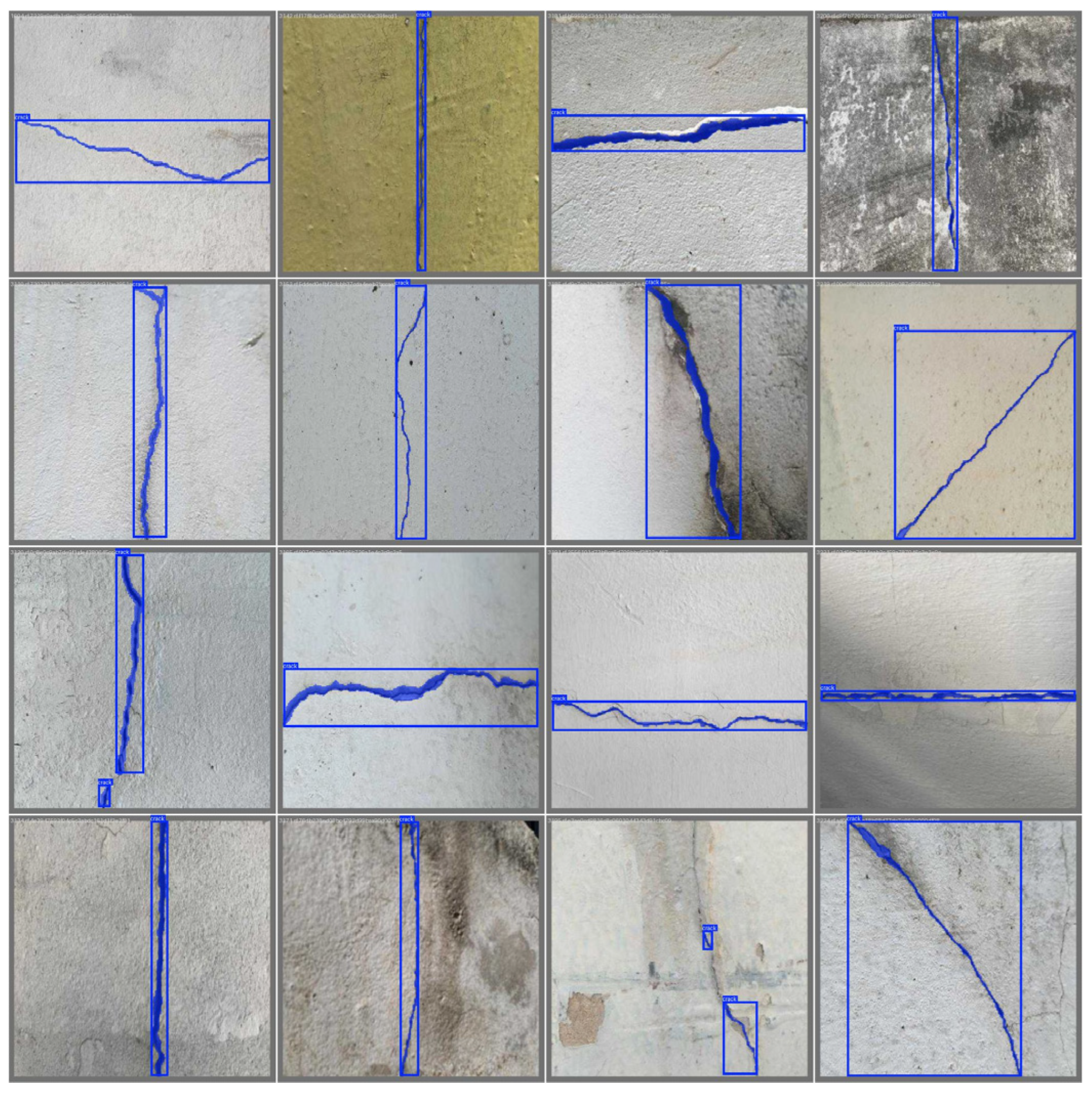
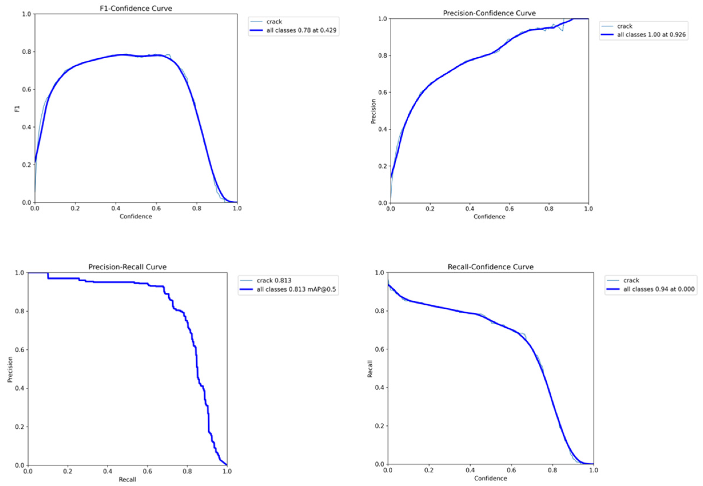
First, we conducted experiments on the selected public dataset. The cracks in this public dataset are more regular and clearer, which is suitable for verifying the feasibility and effectiveness of the method proposed in this paper. As can be seen in Figure 12, the method proposed in this paper can clearly detect the cracks in the public dataset. In Figure 12 and Figure 13, it can be observed that the learning curve gradually converges as the number of samples increases, with a relatively small gap. This indicates that the model neither overfits nor underfits.

Figure 13 shows the recall rate variation trend of the model under different confidence thresholds. As the confidence threshold increases from 0 to 1, the recall rate of the model gradually decreases, and the overall recall rate reaches the highest value of approximately 0.83 at a threshold of 0. It also shows that the precision rate of the model continuously increases with the increase in the threshold under different confidence levels, indicating that higher confidence predictions have higher reliability, with the maximum being 0.926. It also shows the change in the precision rate under different recall rates, and the curve area shows that mAP@0.5 is 0.813. It also shows the change in the F1 value of the model under different confidence levels. The F1 value reaches the highest value of 0.78 when the confidence level is 0.429.

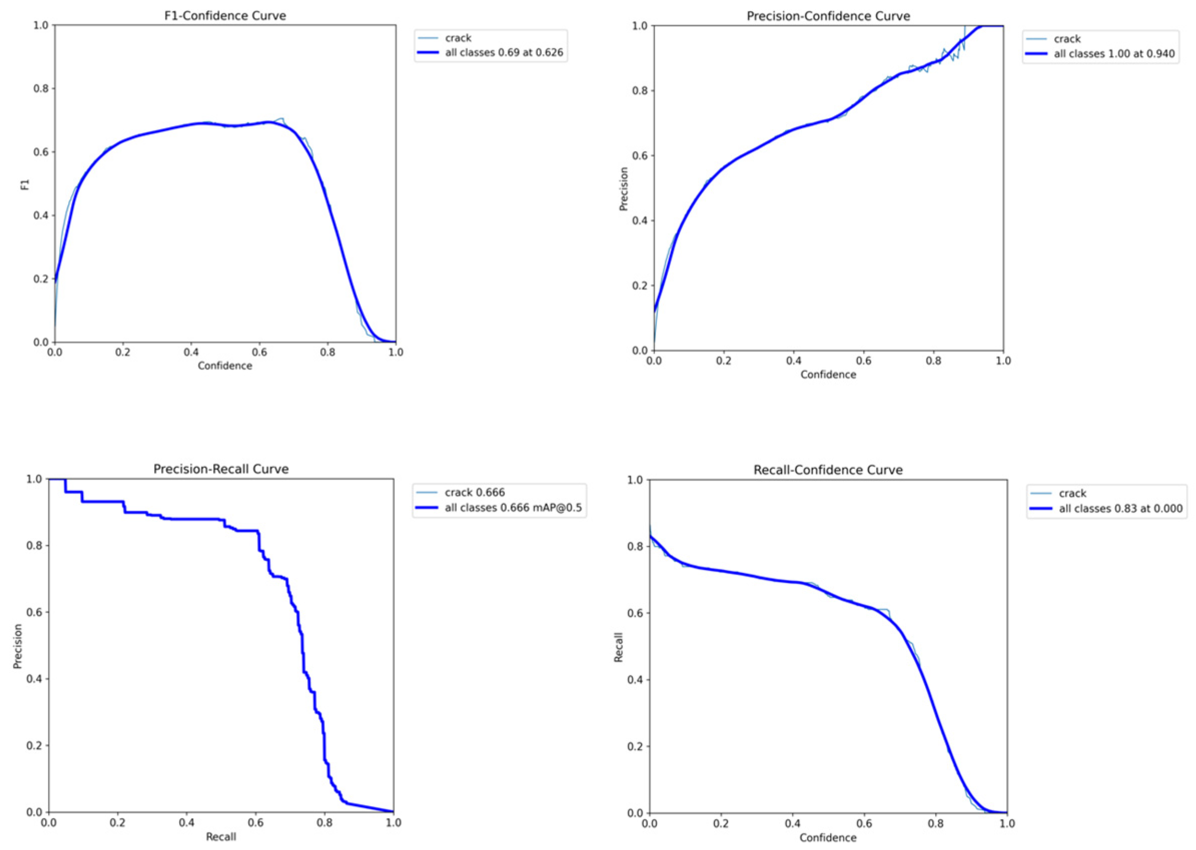
Figure 14 shows the trend of the recall rate of the model under different confidence thresholds. Overall, it reaches the highest recall rate of approximately 0.94 when the threshold is 0. It shows the change in the F1 value of the model under different confidence levels. The F1 value reaches the highest value at 0.69 when the confidence level is 0.626. It shows that the precision rate of the model continuously increases with the increase in the threshold under different confidence threshold levels, reaching the highest value of 0.94. It shows the change in the precision rate under different recall rates. The area of the curve shows that the mAP@0.5 of this model is 0.666.

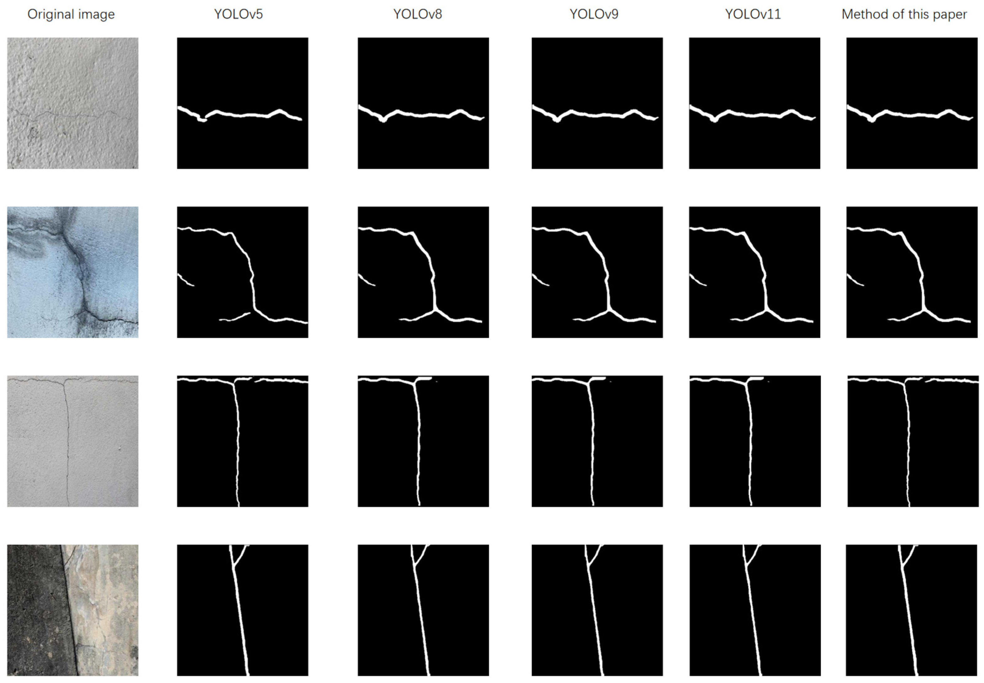
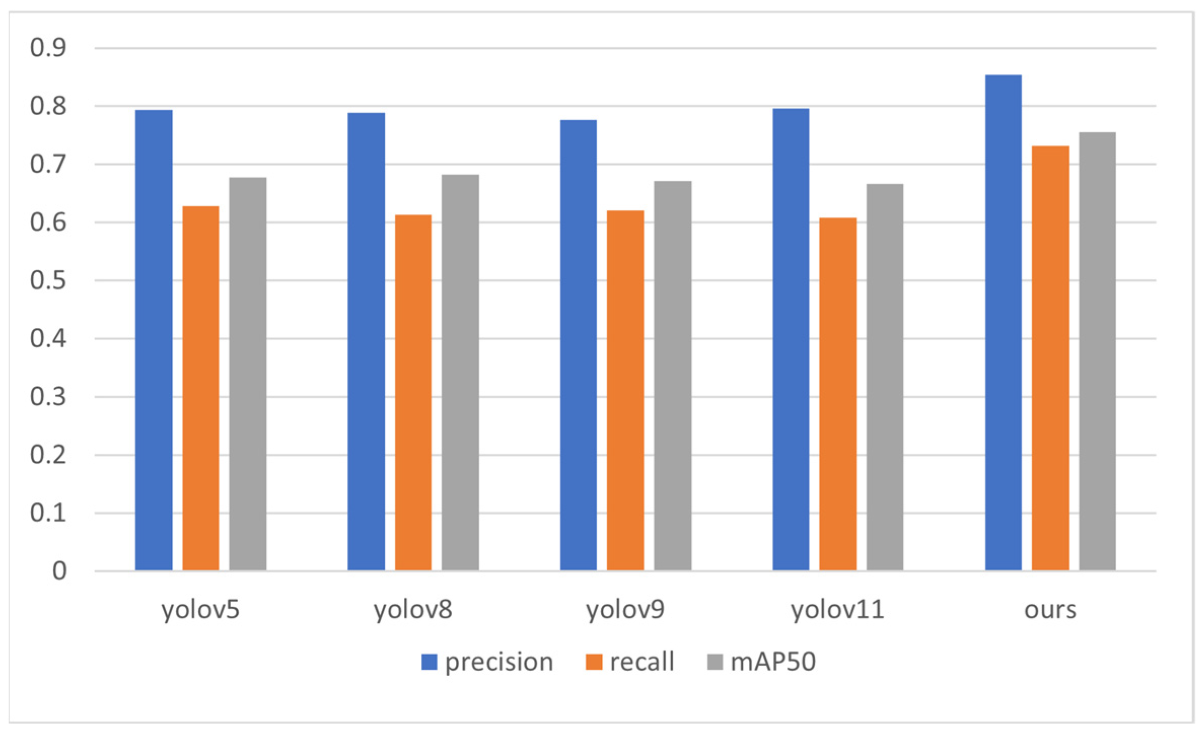
To verify whether the method proposed in this paper is effective and advanced, it is compared with the commonly used yolov5, yolov8, yolov9, and yolov11. Through a comparison of the detection results on the example shown in Figure 15, it is found that this method can effectively detect cracks and extract them over a large area. In

Table 1. Public dataset detection and evaluation indicators.

Method	Precision	Recall	mAP50	Dice Coefficient
Yolov5	0.794	0.628	0.677	0.701
Yolov8	0.789	0.613	0.682	0.689
Yolov9	0.776	0.621	0.671	0.690
Yolov11	0.796	0.609	0.666	0.695
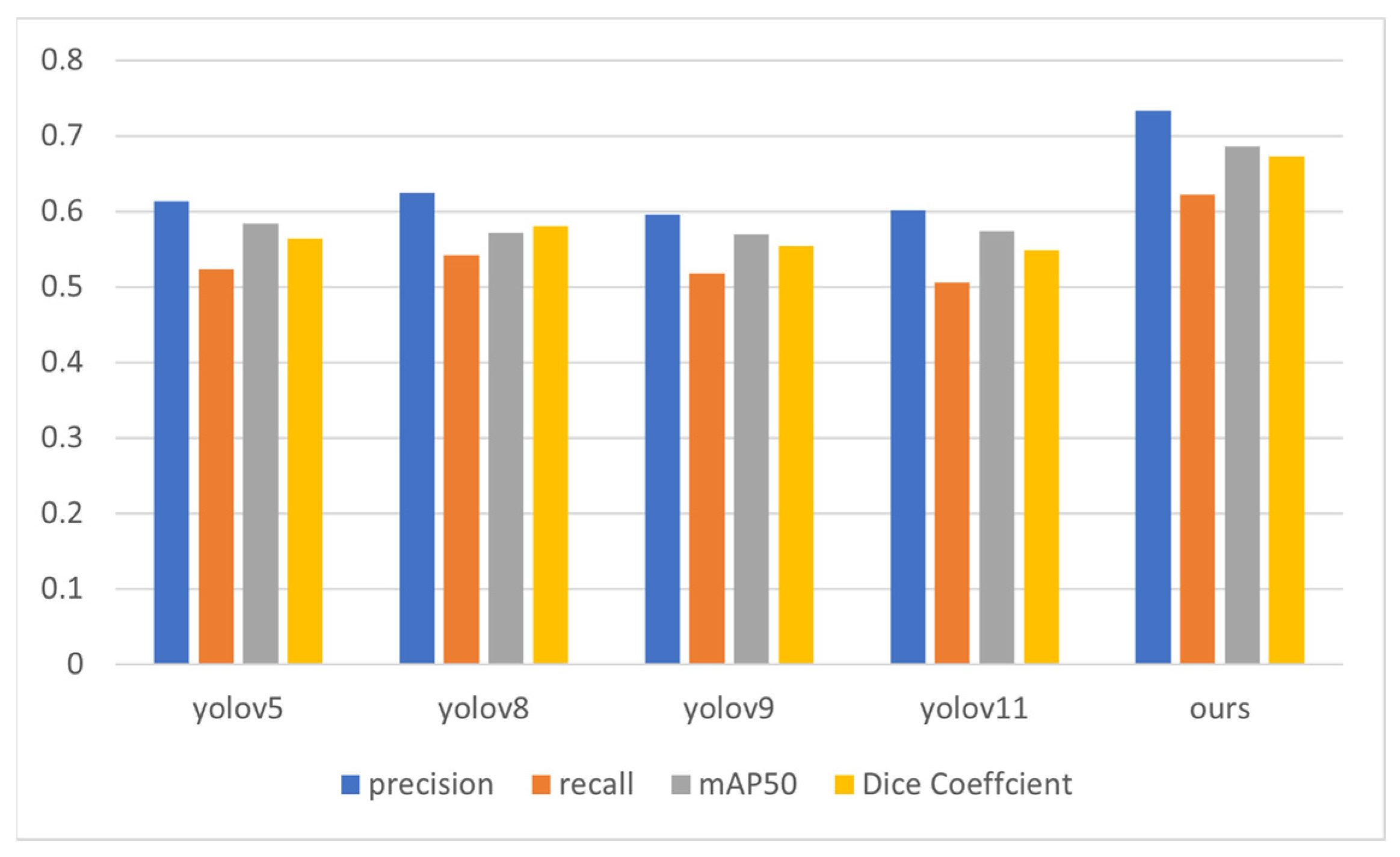
Ours	0.854	0.732	0.756	0.788

, it can be seen that the four evaluation indicators of this method are all higher than those of the other methods, demonstrating that this method is effective and offers certain advancements.

Figure 16 allows for a more intuitive visual comparison of the evaluation indicators obtained after conducting experiments using several different methods. The method presented in this article is more effective than the other methods.

We already conducted experimental verification on the public dataset. Now, we carry out verification on our self-built dataset.

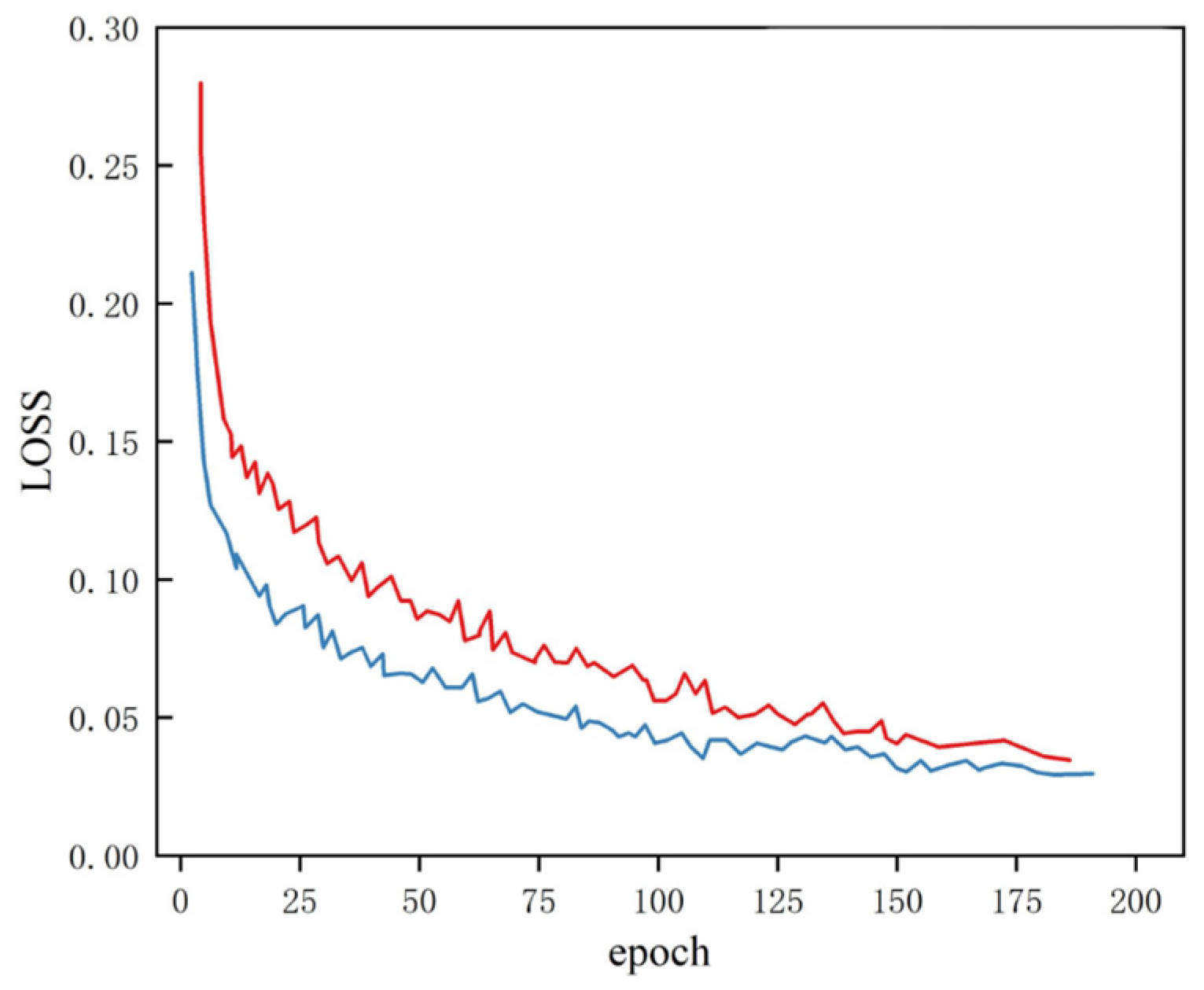
The network’s loss computation comprises three distinct components: the confidence error component evaluates prediction reliability, the bounding box regression component quantifies spatial localization accuracy, and the classification error component measures categorical prediction precision.

A comparative analysis of the convergence patterns in Figure 17 reveals that our optimized algorithm achieves faster convergence with lower stabilized loss values, suggesting enhanced model trainability and improved optimization efficiency through architectural modifications.

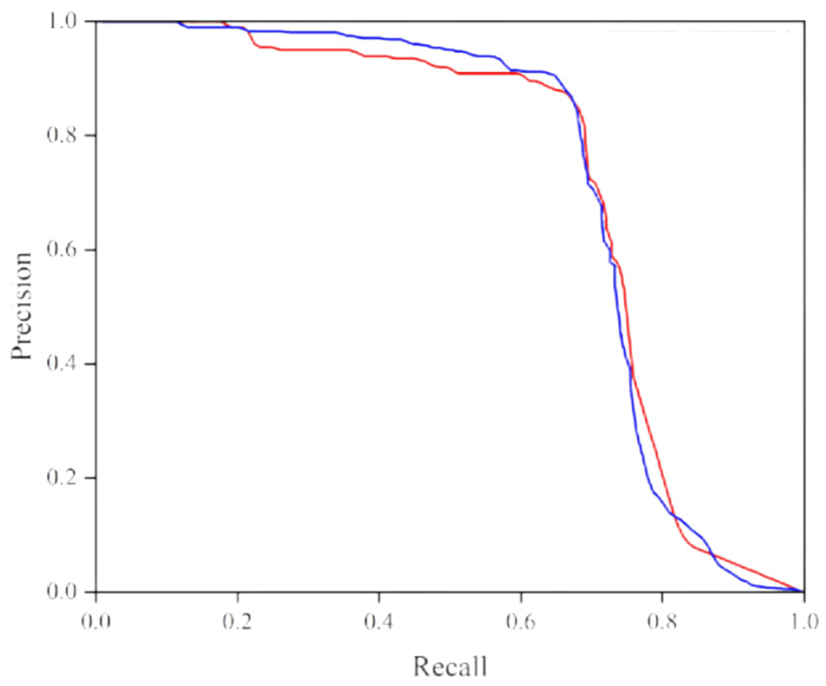
A P-R curve comparison between the enhanced YOLOv5 model and the baseline model is illustrated in Figure 18. A P-R curve positioned nearer to the top signifies superior effectiveness.

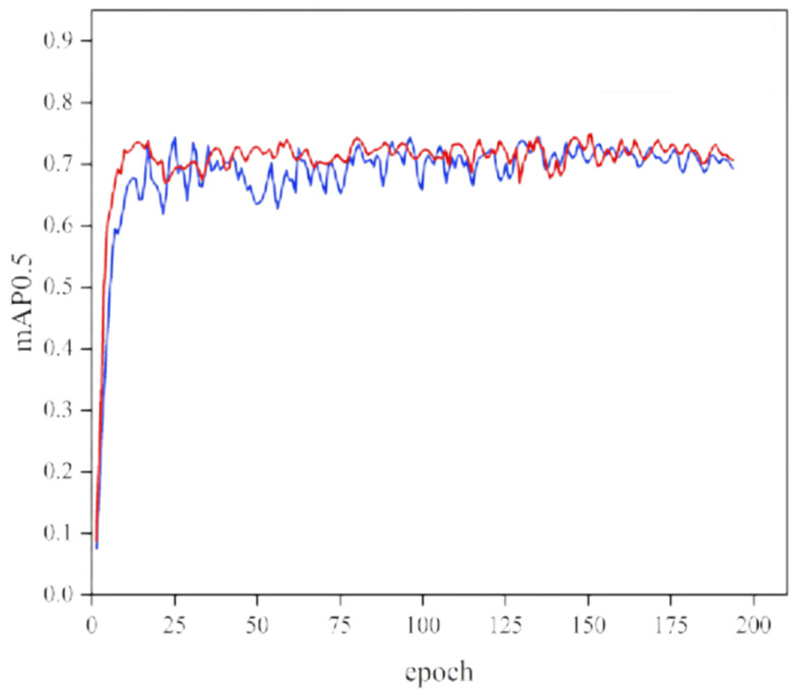
A mAP comparison between the improved YOLOv5 model and the original model is shown in Figure 19. When the threshold is set to 0.5, the average accuracy of the modified YOLOv5 improves.

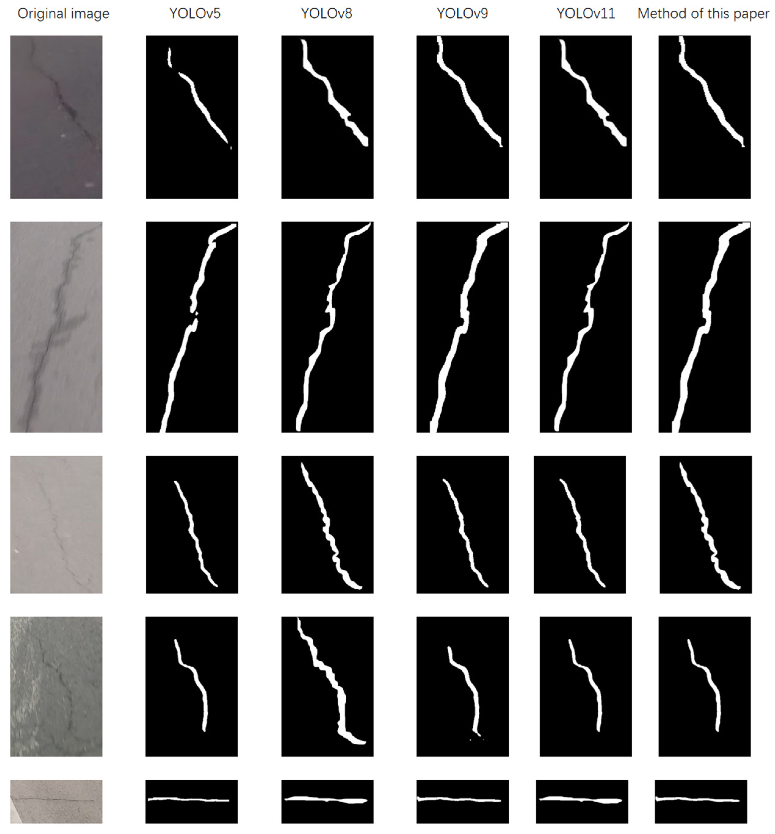
A comparison with the commonly used yolov5, yolov8, yolov9, and yolov11 methods was also conducted. Through a comparison of the detection results in the example diagram shown in Figure 20, it was determined that this method can effectively detect cracks and extract large areas of cracks. As the cracks in the self-built dataset were all captured from driving vehicles, various factors such as angle, light, and speed will have an impact on their detection, so the effect is somewhat reduced. However, when making a horizontal comparison, it can be seen in

Table 2. Comparison of the crack detection results.

Method	Precision	Recall	mAP50	Dice Coefficient
Yolov5	0.613	0.523	0.584	0.564
Yolov8	0.624	0.542	0.572	0.580
Yolov9	0.596	0.518	0.569	0.554
Yolov11	0.601	0.506	0.574	0.549
Ours	0.733	0.622	0.686	0.673

that the four evaluation indicators of this method are still higher than those of the other detection methods used, which is sufficient to prove that this method is effective and offers certain advancements.

Figure 21 allows for a more intuitive visual comparison of the evaluation indicators obtained after conducting experiments using different methods. The method introduced in this paper is more effective than the other methods.

When compared with other methods in the YOLO series, the differences in computational cost and running time are significant, mainly due to the evolution of the architecture and the variation in model size. Compared to our baseline model YOLOv5s, the introduction of the Mish activation function and the EfficientFormerV2 attention mechanism inevitably increases the theoretical computational load (GFLOPs), resulting in an approximately 15–20% decrease in the frame rate (FPS) when running on the same hardware. This is a necessary trade-off that we have made to improve detection accuracy. When compared with more advanced architectures such as YOLOv8, although our model shows advantages in specific tasks, the new-generation models, with their superior overall design, usually achieve higher benchmark performance at similar computational costs. Moreover, model size is the most significant factor affecting resource consumption. Our improved YOLOv5s outperforms large models (such as YOLOv8x) in speed but is slower than lightweight models (such as YOLOv8n). Therefore, model selection essentially involves a comprehensive trade-off between accuracy, speed, and deployment cost. Our method provides a performance-enhanced and well-practiced option for the mature YOLOv5 ecosystem.

4. Discussion

This study proposes a road crack detection method that utilizes deep learning methods in the field of computer science and technology. It is an improvement of the traditional YOLOv5 algorithm, and it uses a new loss function, SIoU; adopts a new activation function, Mish; and uses a new attention mechanism, EfficientFormerV2. This method has strong operability and realizability. It can be seen from the results that, although it has certain advantages, it is not outstanding. Thus, we need to conduct further exploration and incorporate new modules or functions to improve performance.

Road cracks are key indicators of the early health status of the pavement structure. Their timely and accurate detection is of vital importance for infrastructure maintenance and traffic safety. Traditional detection methods mainly rely on manual inspections, which have problems such as low efficiency, high subjectivity, and high safety risks. In recent years, computer vision-based deep learning methods, especially single-stage object detection models such as the YOLO series, have become a research hotspot in this field. Based on the classic YOLOv5 algorithm, this study made a series of targeted improvements to enhance its crack detection accuracy and robustness in complex road scenarios.

Our improvements mainly focus on three core components: the loss function, the activation function, and the attention mechanism. These improvements were not made arbitrarily but were based on a profound understanding of the unique challenges of the crack detection task. We adopted the SIoU loss. SIoU builds upon CIoU and incorporates vector angle considerations by defining the directionality between bounding boxes, enabling the regression process to first attempt to align the axes of the predicted box with those of the real box and then fine-tune them in terms of position and size. The smoothness of Mish gives it better gradient flow, which can alleviate the problem of gradient disappearance and make deep networks easier to train. At the same time, its small information flow retained in the negative half-space helps the model learn richer features, which may have potential benefits for distinguishing cracks from similar shadowy or stained backgrounds, thereby potentially improving the model’s generalization and feature representation abilities. We integrated EfficientFormerV2, which is a lightweight network specifically designed for visual tasks, with a pure Transformer architecture. We embedded it as an attention module into the backbone network of YOLOv5. EfficientFormerV2 can efficiently establish long-distance dependencies in images. In crack detection, this means that the model can better understand the global context.

Compared with the baseline YOLOv5, our model achieved a significant improvement in the mAP@0.5 metric. Especially in the detection of small cracks and cracks in complex backgrounds, the false-negative and false-positive rates both decreased. This verifies the effectiveness of the combination of SIoU, Mish, and EfficientFormerV2. Our method leverages the speed advantage of single-stage detectors while maintaining comparable to or even better accuracy than them, which better meets the real-time requirements of road inspection. Our model training is more stable, converges faster, and has lower requirements for computing resources, demonstrating the superiority of embedding a lightweight Transformer as a module into the CNN architecture.

Generalization capability bottleneck: The performance of the model is highly dependent on the distribution of the training data. Models trained under specific lighting conditions or on specific road surface materials (such as asphalt) may exhibit a sharp decline in performance when faced with night conditions, post-rain reflections, cement roads, or cracks covered by dust or vegetation. The diversity and coverage of the dataset are some of the biggest challenges currently faced. Insufficient handling of extreme and ambiguous cases: For extremely fine hair-like cracks, low-contrast cracks that blend with the road texture, or severely obscured cracks, the recall rate of the model is still not high. This is due to the reliance of deep learning models on “significant” features, while the characteristics of these cases are not significant. Trade-off between computing resources and real-time performance: Although EfficientFormerV2 improves efficiency, the introduction of Mish and more complex attention mechanisms still increases the computational load. On resource-constrained edge devices (such as the embedded Jetson platform on inspection vehicles), to achieve stable high-frame-rate (such as >60 FPS) processing of high-definition video streams, optimization steps such as model quantization and pruning are still required. The “false-positive” problem in practical applications: In complex real road environments, road joints, tire marks, oil stains, shadows, etc., may all be misjudged by the model as cracks. An excessively high false-positive rate will significantly increase the cost of manual review and even cause the system to lose the trust of users. How to design more refined post-processing algorithms or introduce multimodal data (such as infrared, 3D point clouds) for fusion verification is an urgent problem to be solved. The gap from “detection” to “evaluation”: Current models only complete the task of “marking cracks”, but road maintenance decisions require quantitative evaluation information such as that pertaining to the length, width, area, and type (transverse, longitudinal, or mesh-like) of cracks. This requires an evolution from target detection to more fine-grained tasks such as instance segmentation or keypoint detection.

5. Conclusions

Road surface fractures represent a primary hazard affecting pavement integrity, necessitating advanced identification approaches for effective infrastructure maintenance. Contemporary research in fracture recognition has shown substantial advancements through deep learning applications. To enhance algorithmic efficiency in both accuracy and processing speed, this study introduces an enhanced YOLOv5-based framework for pavement defect identification. In the proposed methodology, structural modifications are made to the conventional YOLOv5 architecture, demonstrating improved practical applicability and processing efficiency through comprehensive experimental validation. Comparative analyses reveal that this approach achieves notable enhancements in detection precision and operational velocity compared to baseline models. Future research will focus on refining this methodology to attain superior performance metrics through continuous algorithmic optimization.

The precision, recall, mAP50, and Dice coefficient values in this paper demonstrated certain advantages when compared with those of other methods, whether obtained on public datasets or on self-built datasets. A better balance is achieved between detection accuracy and speed, verifying the feasibility and value of algorithm optimization for specific tasks. It provides a solid technical foundation for building an automated and intelligent road inspection system. Future research will focus on the following: Exploring stronger backbone networks: Attempts will be made to integrate more advanced versions of YOLO (such as YOLOv9) or pure Transformer architectures to pursue higher performance limits. Data augmentation and generation: Generative adversarial networks (GANs) or diffusion models will be used to generate diverse crack samples, enhancing the model’s generalization ability at a low cost. Multi-task learning: Crack detection, segmentation, and classification tasks will be integrated into a unified framework to achieve the transition from “whether there is” to “what and how it is”. Edge computing optimization: In-depth studies on model compression techniques will be conducted to ensure that the algorithm can run efficiently on low-power devices, truly realizing the intelligent inspection system of “cloud-edge-end” collaboration.

In conclusion, the path to intelligent road crack detection is still long, requiring the deep integration and continuous exploration of algorithms, data, hardware, and application scenarios.