Article

The Effect of Data Augmentation on Performance of Custom and Pre-Trained CNN Models for Crack Detection

1
Department of Civil Engineering, Nigerian Army University Biu, Biu 603108, Nigeria
2
Department of Mechanical Engineering, Nigerian Army University Biu, Biu 603108, Nigeria
3
Department of Civil Engineering, ARISE, ISISE, University of Minho, 4800-058 Guimarães, Portugal
*
Author to whom correspondence should be addressed.
Appl. Sci. 2025, 15(22), 12321; https://doi.org/10.3390/app152212321
Submission received: 12 October 2025 / Revised: 15 November 2025 / Accepted: 18 November 2025 / Published: 20 November 2025
(This article belongs to the Section Civil Engineering)

Abstract

Data augmentation is one of the effective solutions to improve the performance of machine learning models in general and deep learning in particular. Data augmentation techniques bring different effects to each model, but very few studies have considered this issue. This study investigated the effect of five distinct data augmentation strategies on a custom-built Convolutional Neural Network (CNN) and nine pre-trained CNN models for crack detection. All ten models were initially trained on a reference dataset of unaugmented images, followed by separate experiments using the augmented datasets. The results show that the pre-trained models, especially VGG-16, EfficientNet-B7, Xception, DenseNet-201, and EfficientNet-B0, consistently achieved greater than 98% in accuracy across all augmentation techniques. Meanwhile, the custom-built CNN was very sensitive to illumination changes and noise. Image rotation and cropping have minimal negative impact and sometimes improve performance. The findings demonstrate that combining data augmentation with state-of-the-art pre-trained models offers a powerful and efficient alternative to the reliance on large-scale datasets for accurate crack detection using CNNs.

1. Introduction

Early detection of cracks in infrastructure is crucial for timely repairs, preventing further deterioration and potential total collapse. Visual inspection (VI) is one of the oldest and most common methods of crack detection, especially at the surfaces. While visual inspection is relatively easy to undertake, it is highly subjective, time-consuming, and poses a significant risk to inspectors when inspecting hard-to-reach areas [1]. The emergence of artificial intelligence (AI), however, has generated significant interest in deep-learning-based crack detection as a viable alternative to VI. One widely popular and effective deep learning (DL) method suitable for image-based cracks or defect detection is the convolutional neural network (CNN) algorithm. The main strength of CNN is its ability to self-learn by extracting features from images, making it well-equipped for the task of crack detection and minimizing the need for manual inspection [2]. Compared to classical computer vision approaches, CNNs have demonstrated superior accuracy, generalization, and robustness across various datasets and defect types. Research also finds that CNN models are faster and more consistent than manual inspections, making them ideal for real-time infrastructure monitoring [3,4,5,6].
Although CNNs have achieved significant successes in damage detection, the associated cost of acquiring and processing image data for CNN crack/damage detection is significant, accounting for 80–90% of the overall cost; therefore, a major drawback in its implementation is the requirement for large amount of labeled and diverse image data for effective training and to prevent underfitting [7]. Underfitting occurs when a CNN model fails to sufficiently learn the underlying pattern in the data, leading to inaccurate predictions, particularly with unseen datasets. To prevent this, transfer learning and data augmentation are proven strategies. These techniques have been applied and proven effective in many models. Transfer learning utilizes already trained models, which are then fine-tuned to fit the task objective. Transfer learning techniques allow the model to generalize better and avoid overfitting. Meanwhile, data augmentation uses basic transformations to create new data. From there, the model has more data to learn and achieves better generalization [8].
For transfer learning techniques, the models used have been trained on a huge amount of image data (e.g., ImageNet). This data includes millions of images with specific labeled object categories. Because they are trained on large data, these models already have a high generalization ability. They can easily recognize the target in the given task. However, before being used, the model needs to be fine-tuned to fit the task datasets. Instead of training a model from scratch, which requires substantial computational resources and a large dataset, this method enables the creation of a new model with high generalization ability while utilizing significantly smaller resources. This method significantly reduces training time, improves generalization ability, and has been shown to provide higher accuracy even on limited datasets [9]. Common examples include VGG-16, ResNet-50, Inception-V3, EfficientNet, and DenseNet.
On the other hand, data augmentation has emerged as a highly effective strategy for improving model generalization and performance across a wide range of machine learning domains. A summary of these methods is shown in Figure 1. While it is most often associated with computer vision tasks, which involve geometric and photometric transformations of images, its applications extend far beyond visual data. In natural language processing (NLP), augmentation techniques such as synonym replacement, random insertion, and back-translation have been shown to improve sentiment analysis and text classification tasks. In speech and audio processing, pitch shifting, time stretching, and background noise injection are also commonly used to increase model robustness in speech recognition and speaker identification. In time series analysis, data augmentation solutions significantly support model performance. Specifically, augmentations such as adding Gaussian noise, shifting, or rescaling can make models immune to noise and measurement errors. Even in biomedical signal processing, data augmentation for electrocardiogram (ECG) or EEG data has been shown to be effective in improving model reliability on small datasets. Recent survey papers such as [10,11,12,13] have detailed the breadth of augmentation techniques used across these fields.
In crack detection, specifically, several studies have demonstrated the effectiveness of data augmentation in improving model performance in scenarios where data is scarce, with basic geometric augmentations such as horizontal and vertical flipping, rotation, cropping, and scaling being among the most commonly used techniques [10]. These help CNNs learn invariance to orientation and position, which is critical since cracks can appear at any angle or part of a structure. For instance, Gu et al. [14] demonstrated that combining data augmentation with hyperparameter tuning significantly enhanced CNN performance on the CIFAR-10 dataset. The approach reduced overfitting and improved VGG16 test accuracy to 92%, while t-SNE visualizations further confirmed clearer class separation due to augmentation. Similarly, Kim and Cho [15] employed data augmentation to address the limited diversity of images used in training the AlexNet model, which contains over 60 million parameters. Hence, they ultimately expanded the dataset size by up to tenfold and significantly reduced overfitting.
Similarly, photometric augmentations, such as brightness adjustment, contrast variation, and gamma correction, introduce variability in lighting conditions. These are especially helpful in simulating real-world conditions where shadows, reflections, or uneven illumination may otherwise degrade model performance [16]. Osman et al. [17] applied CLAHE (Contrast Limited Adaptive Histogram Equalization) to enhance pavement crack images before training VGG16 and a nine-layer CNN. Contrast enhancement significantly improved the performance of the models. Accuracy increased to 99.6 and 99.1%, outperforming raw unprocessed images. Researchers have leveraged this to explore additional noise-based enhancement techniques. The methods significantly enhance the performance of data from sensors with limited or poor image quality. These methods enhance model robustness in low-quality or UAV-acquired images, as shown by Nguyen et al. [18]. To overcome overfitting issues suffered by deep neural networks when faced with noisy datasets, Zhang et al. [19,20] proposed a sample selection method that utilized the loss function or training dynamics to distinguish between clean and noisy datasets. The main idea is for the deep neural network to fit the clean data first, while the loss values for noise datasets remain high or fluctuate significantly during the early stages of training.
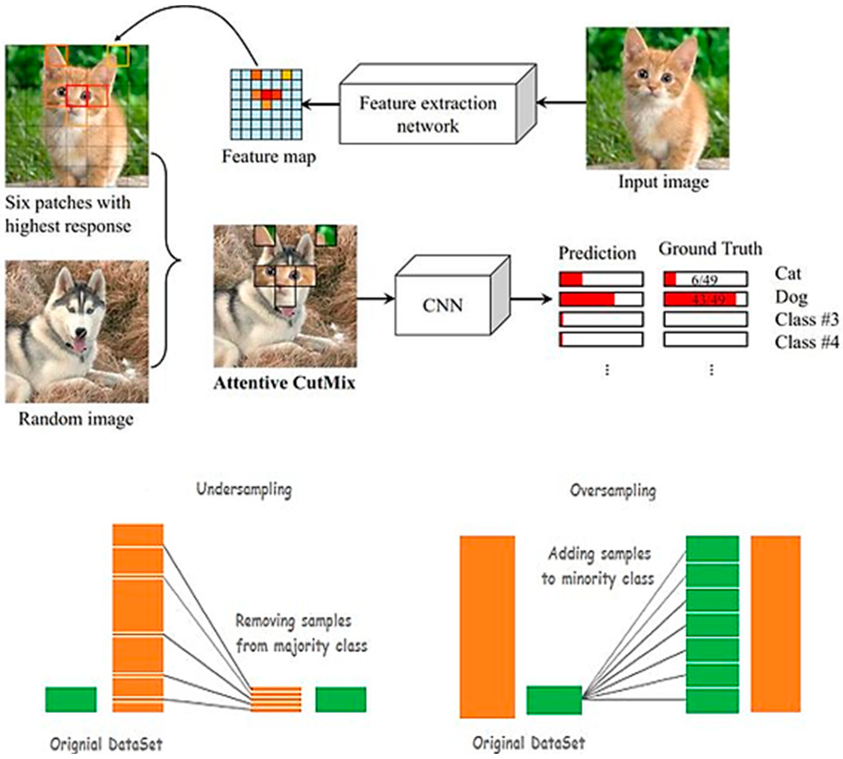
Some researchers have also experimented with synthetic data generation using generative adversarial networks (GANs) or traditional rendering tools to create artificial crack images. While computationally intensive, these methods provide additional flexibility in simulating rare or severe crack conditions [21,22]. Similarly, Choi et al. [23] combined real-world images with synthetically generated data from a 3D virtual environment. Their method automated both image creation and annotation using mask-based rendering, and the resulting hybrid dataset improved their model performance, increasing the F1-score by 10% compared to using real image augmentation alone and by 4.4% over virtual images alone. Other novel data augmentation techniques which have proven highly effective for addressing imbalanced datasets include the region-based techniques like CutMix and MixUp (see Figure 2), which involve blending or patching together different training images or labels to encourage the model to focus on more diverse features [24], and the SMOTE (Synthetic Minority Oversampling Technique), a data augmentation technique that generates new synthetic samples by interpolating between existing minority class samples [25].
The effectiveness of data augmentation will vary depending on the type and quality of the original dataset. Similarly, the choice between training a custom model from scratch and fine-tuning a pre-trained model depends on factors such as dataset size, computational resources, and task-specific requirements [16]. Given these considerations, this study aims to systematically evaluate the effect of data augmentation on the performance of both a proposed lightweight CNN and a set of pre-trained models. To achieve this, we employed nine widely recognized pre-trained CNNs, each renowned for its prowess in image classification and transfer learning. These models span a range of architectural depths and complexities, offering diverse learning capacities and inference efficiencies.
VGG16, developed by the Visual Geometry Group at Oxford, is renowned for its straightforward, uniform 16-layer structure, which stacks 3 × 3 convolutional layers with max pooling and fully connected layers. While computationally intensive, its simplicity and robust feature extraction make it a classic choice for tasks like crack detection, where fine textures are critical [28]. Building on this, He et al. [29] developed ResNet50 which introduces residual connections to tackle the vanishing gradient problem, enabling the training of much deeper networks [29]. Unlike VGG16, its skip connections facilitate identity mappings, striking a balance between depth and performance, and making it a popular option for civil infrastructure defect detection.
Expanding on architectural innovation, InceptionV3 by Google incorporates inception modules—parallel filters of varying sizes—to extract multi-scale features efficiently [30]. Meanwhile, EfficientNet-B0 leverages compound scaling to optimize depth, width, and resolution simultaneously, while its larger counterpart, EfficientNet-B7, pushes this scaling further for higher accuracy, albeit with increased computational demands [30,31].
DenseNet201 stands out for its ability to connect each layer to every other layer in a feed-forward fashion, promoting feature reuse and mitigating vanishing gradients. This allows the model to learn better and avoid forgetting details [32,33]. On the other hand, Xception, an evolution of the Inception family developed by François Chollet [34], employs depth-wise separable convolutions for greater efficiency, making it excellent in tasks where channel-wise spatial features are significant. InceptionResNetV2 merges the strengths of inception modules and residual connections, enabling very deep learning with manageable complexity and achieving top-tier performance in large-scale image classification [30], while the ResNet152V2, an enhanced version of ResNet, boasts 152 layers and improved normalization, a remarkable depth that enables it to capture highly complex patterns, especially when augmented data is used [35].

2. Materials and Methods

2.1. Dataset Description

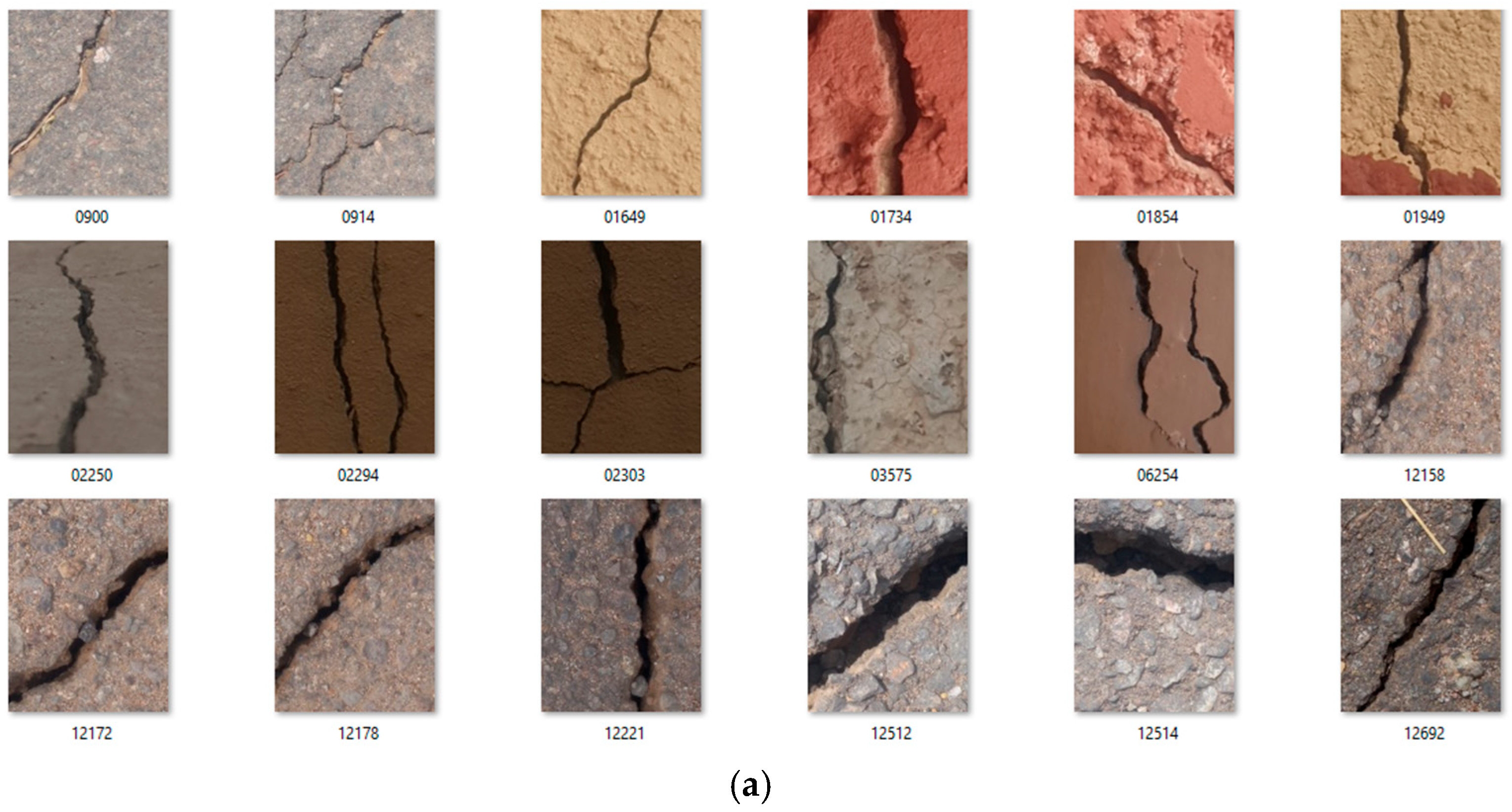
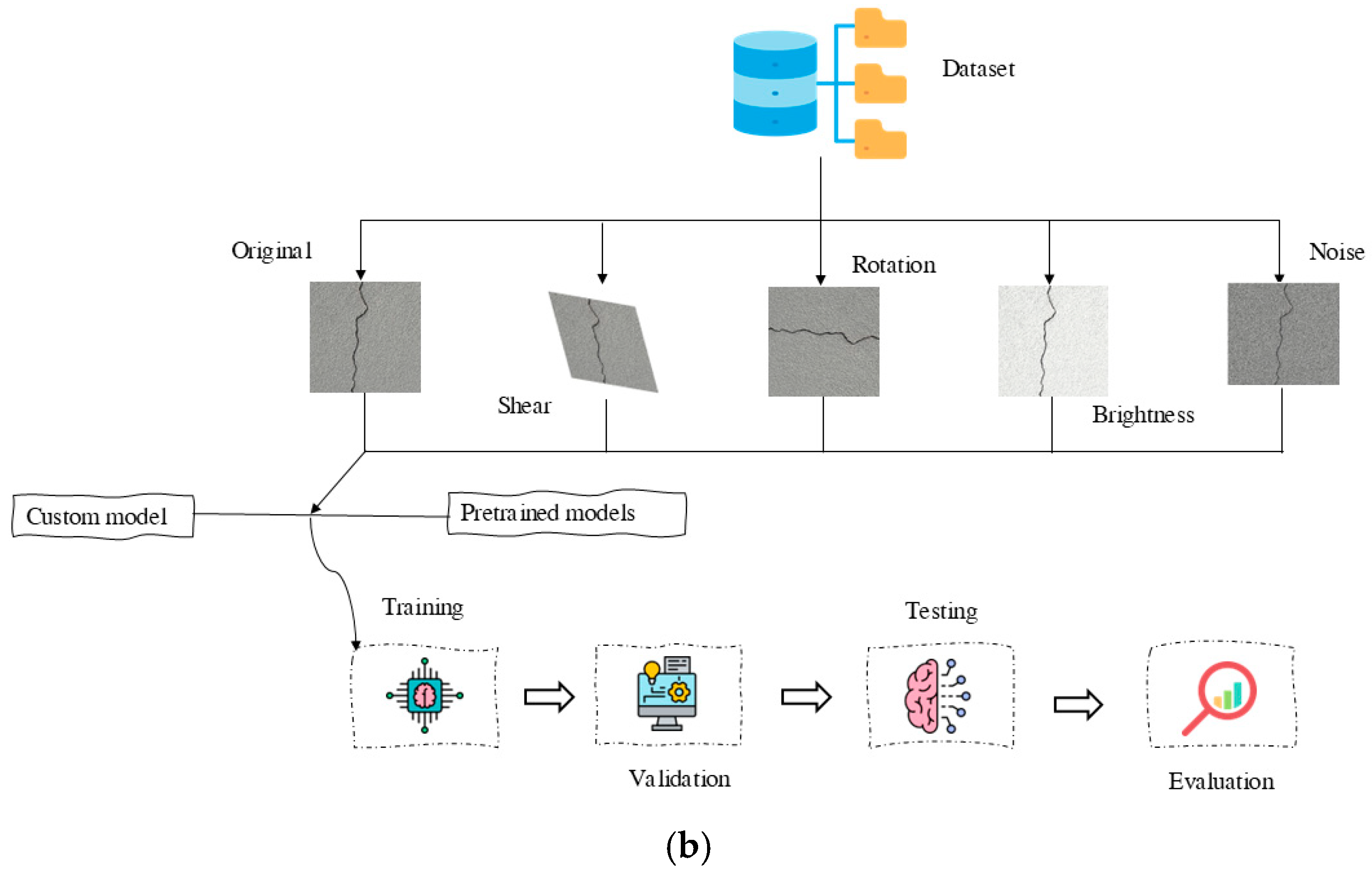
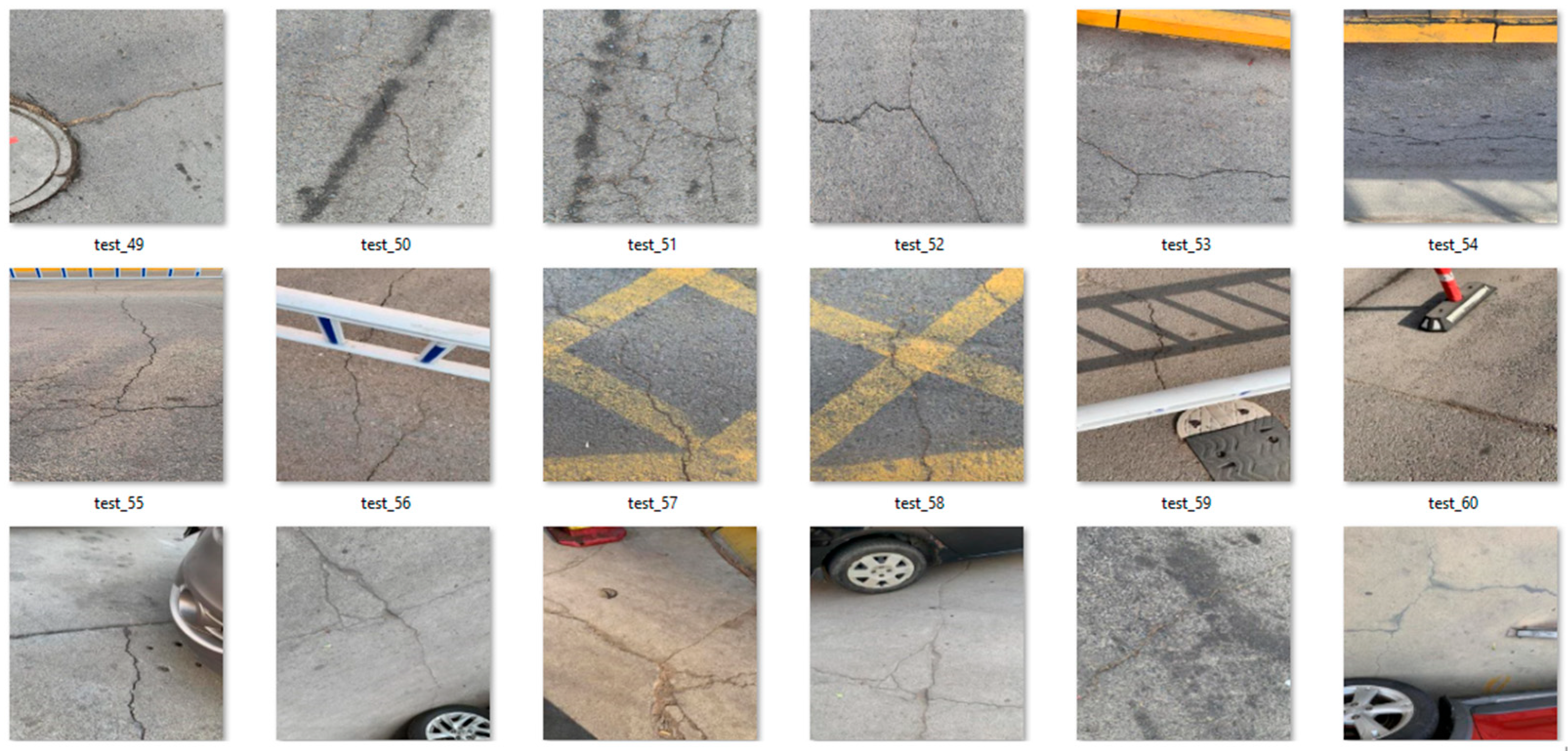
The dataset used in this study was adopted from Omoebamije et al. [2], comprising approximately 32,500 high-resolution images of concrete surfaces. It was developed for a binary classification task: crack versus no crack, and the images were curated across diverse structures (buildings, road pavements, drainages, etc.), ensuring a diverse mix of crack patterns, surface textures, and lighting conditions. All images were resized to 120 × 120 pixels to standardize input dimensions across both the custom-built and pre-trained CNN models. Figure 3a,b shows some representative samples of images used and the general workflow adopted in the study, respectively.

2.2. Data Augmentation

To evaluate how data augmentation affects crack detection performance, the dataset was split into 15,000 training and 2500 testing images without augmentation. In separate trials, 3750 augmented images were used for training, while the test set and validation split (25%) remained unchanged. A targeted augmentation pipeline was applied to the training set to simulate real-world image variability and improve model generalization. The augmentations implemented include shear (±10°), rotation (±15°), brightness adjustment (±20%), Gaussian noise injection (0.25%), and blurring (2.5 px), all executed using the Roboflow workspace.

2.3. Model Implementation and Training

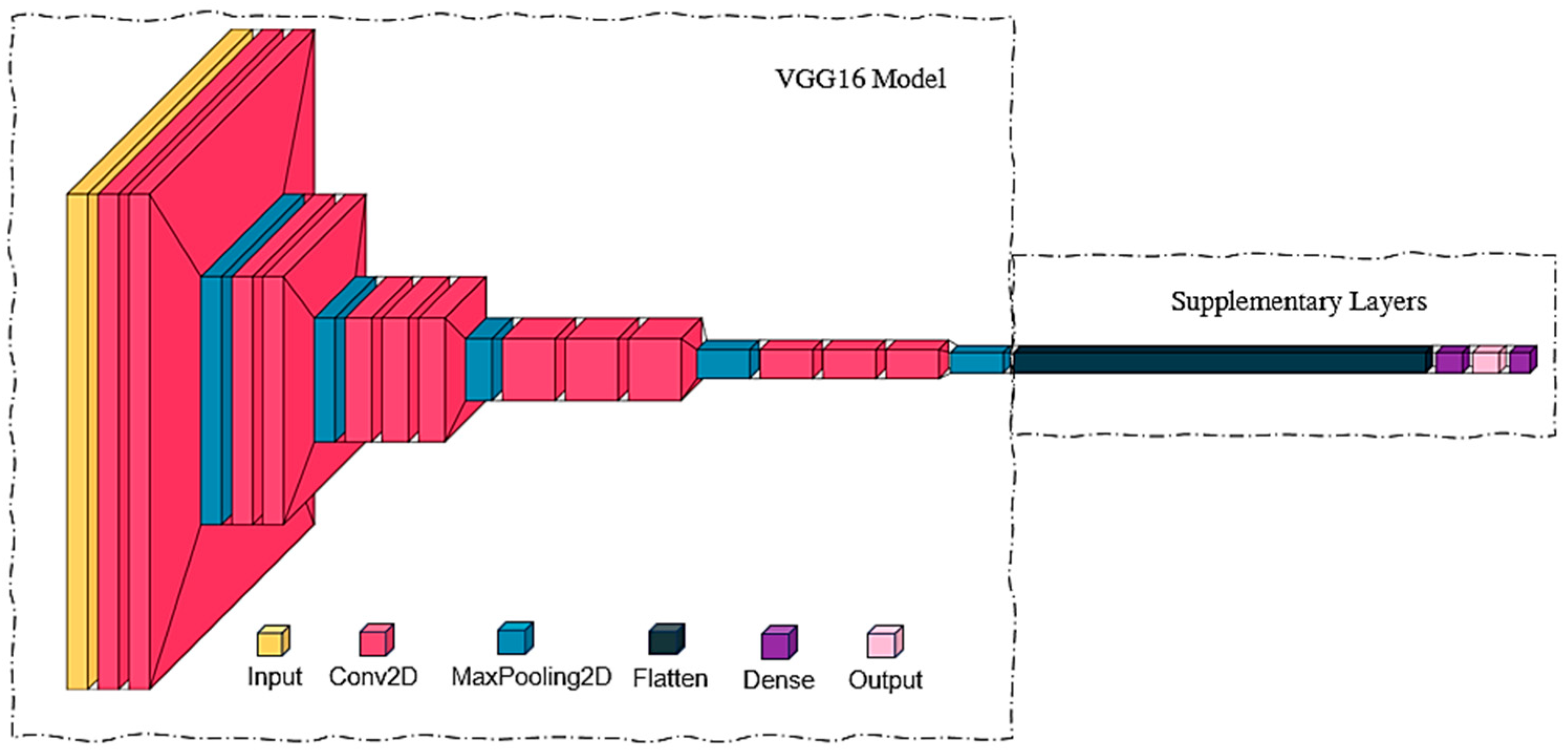
This study adopted a dual-path approach involving the adoption of a lightweight custom convolutional neural network (CNN) from Omoebamije et al. [2] and the fine-tuning of nine widely used pre-trained CNN architectures for binary crack classification. The custom CNN model comprises three convolutional layers, each preceding a max-pooling layer, all flattened into a fully connected layer using SoftMax activation for binary classification between crack and no-crack cases. In parallel, nine pre-trained models, VGG16, ResNet50, InceptionV3, EfficientNet-B0, EfficientNet-B7, ResNet152V2, DenseNet201, Xception, and InceptionResNetV2, were all employed and fine-tuned for transfer learning. For each model, the final output layer was replaced with a fully connected layer tailored to the binary classification task (crack or no crack), incorporating dropout and batch normalization layers to reduce overfitting, as depicted in Figure 4.
All models were trained with the Adam optimizer, learning rate 0.00001, and batch size 128. Meanwhile, binary cross-entropy served as the loss function. The number of training epochs was set to 20. However, all layers in the pre-trained models were initially frozen for the first 10 epochs, and only the last four layers were thawed for fine-tuning in the last 10 epochs. The goal of this was to stabilize the learning process of the model. The environment used to implement the experiments was Google Colab Pro, using a virtual machine equipped with an NVIDIA Tesla T4 GPU (16 GB GDDR6 memory), 52 GB RAM, and a 2-core Intel Xeon CPU @2.30 GHz. The software environment included Python 3.13, TensorFlow 2.18, and Keras 3.9.0. In addition, training was performed in the Jupyter Notebook environment using the Keras API.

2.4. Evaluation Metrics

To evaluate the models’ performance, the following metrics were employed on the test dataset:
i 
Accuracy (A): This reflects the overall correctness of predictions and is defined as: A = T P + T N T P + T N + F P + F N
where TP = True Positives, TN = True Negatives, FP = False Positives, and FN = False Negatives.
ii 
Precision (P): This is a measure of the proportion of correctly identified crack instances among all predicted as cracks: P = T P T P + F P
iii 
Recall (R): This is also called sensitivity, and it quantifies the model’s ability to capture all actual crack instances: R = T P T P + F N
iv 
F1-score: This is a measure of a test’s accuracy, defined as the harmonic mean of its precision and recall values: F1-score = 2 P R P + R
v 
Confusion Matrix (CM): The confusion matrix provides a detailed breakdown of the model’s classification results, showing the counts of true positives, false positives, true negatives, and false negatives.
These metrics were computed using the same fixed test set of 2500 images. For completeness, confusion matrices, Receiver Operating Characteristics (ROC) curves, and Precision-Recall (PR) curves were also plotted for both the custom and pre-trained CNN models, enabling a robust assessment of their classification performances.

3. Results

Model Training Patterns

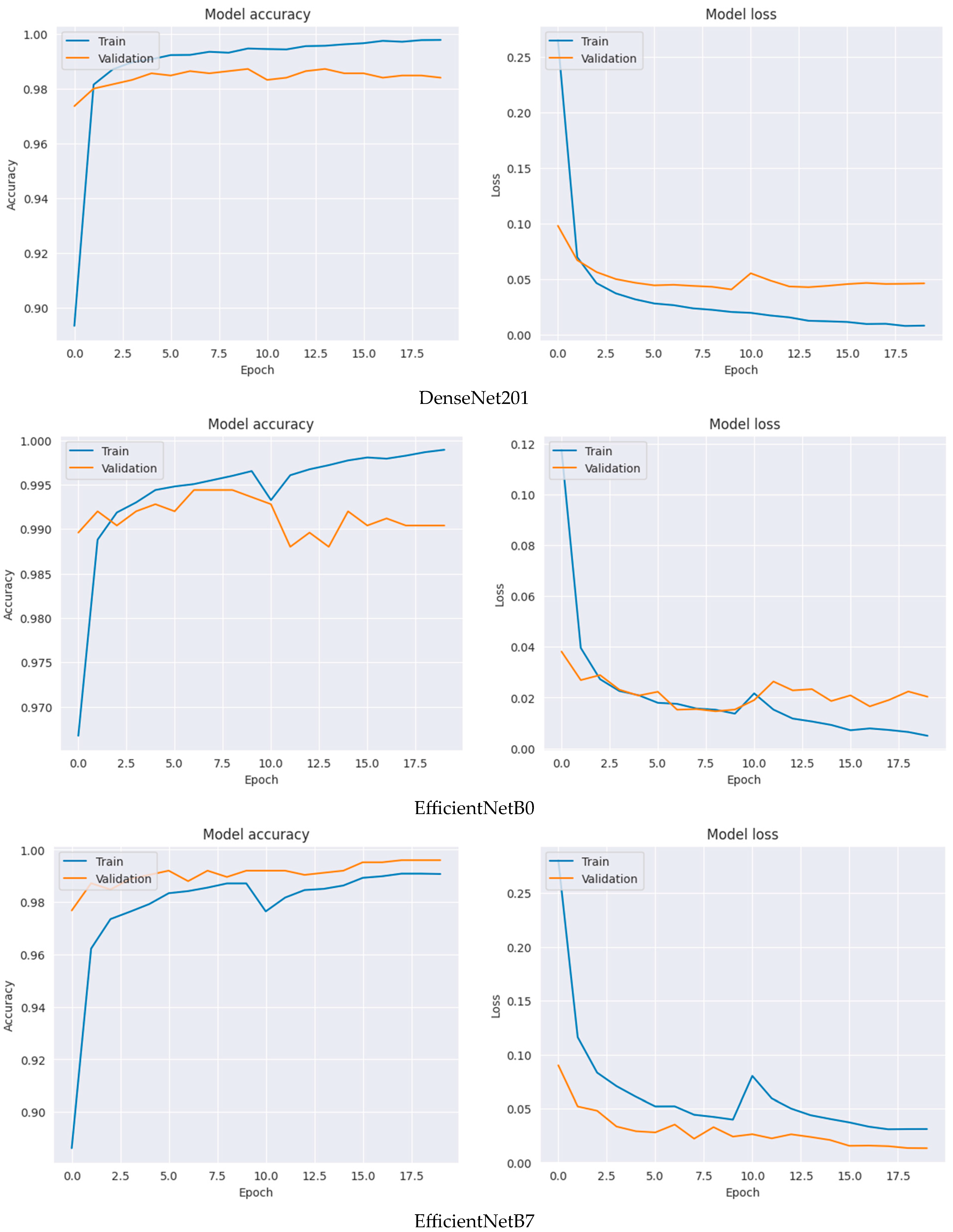
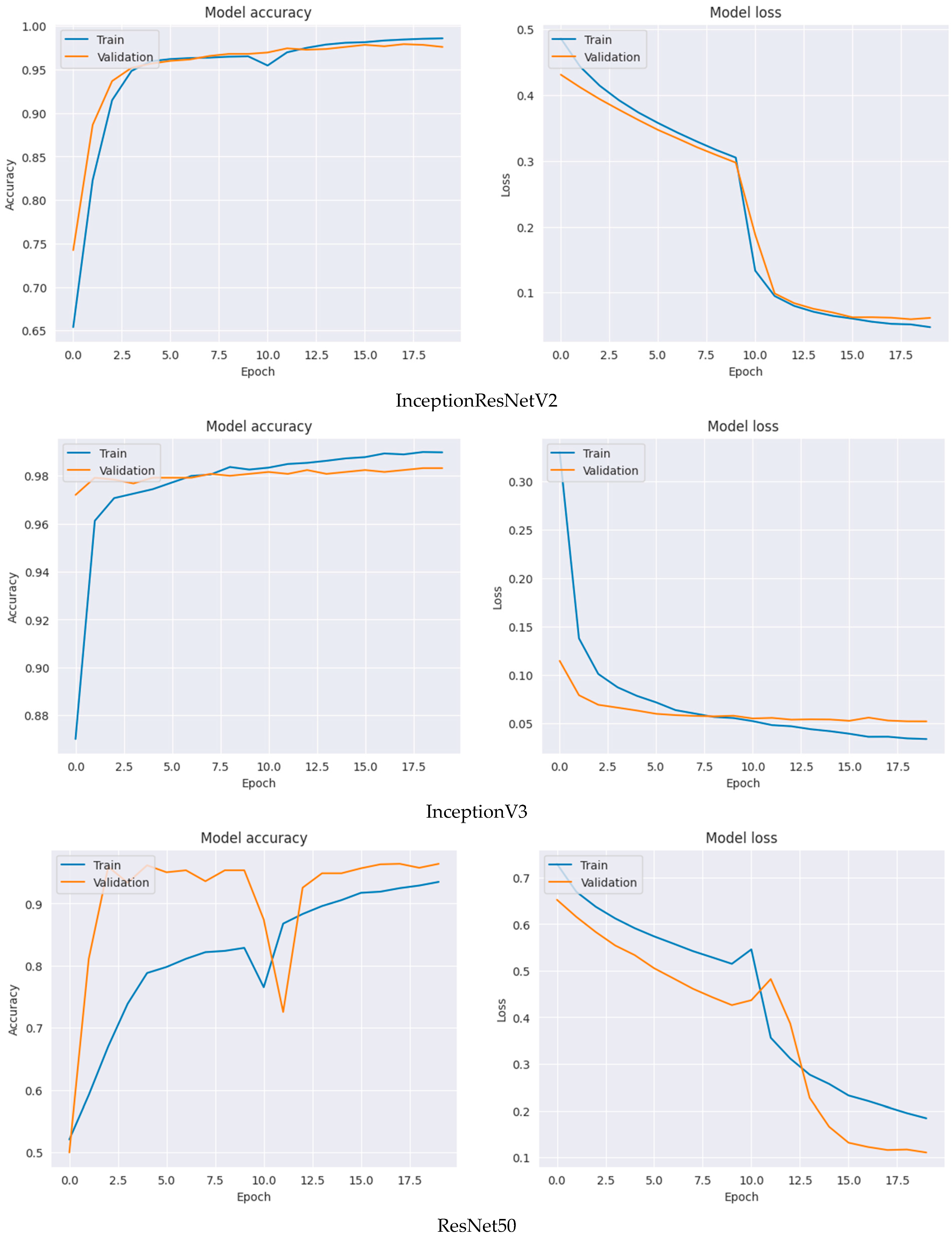
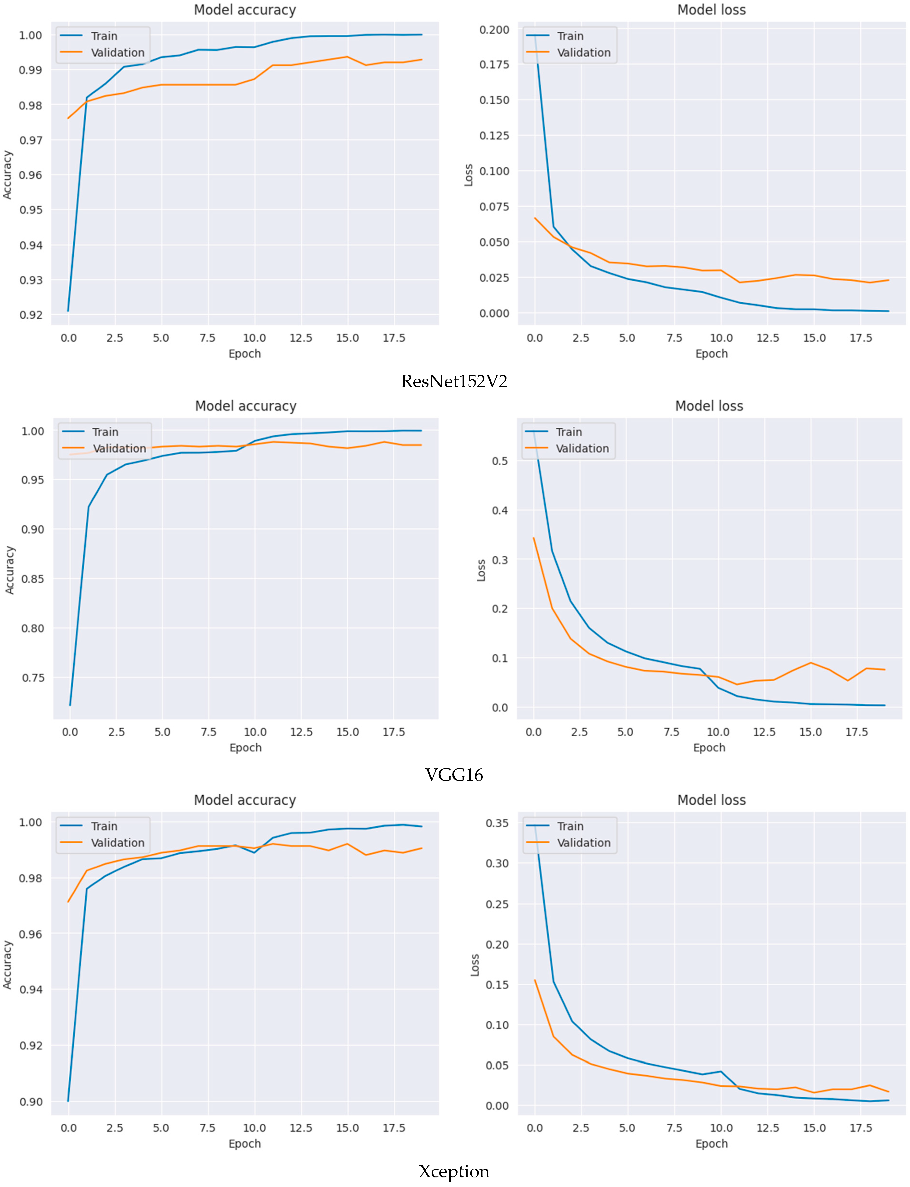
The behavior of the model during training on the baseline dataset (without augmentation) and the augmented dataset is evaluated using the plots of the model’s accuracy and loss for both training and validation datasets. Figure 5, Figure 6 and Figure 7 show these plots for the baseline dataset. As can be seen in these figures, the training accuracies of VGG-16, InceptionV3, InceptionResNetV2, ResNet152V2, and Xception gradually increase, reaching 98.5%, 98.3%, 97.6%, 99.3%, and 99.0%, respectively. Also, the validation accuracy mirrors closely the training accuracy. Equally, training and validation losses showed a consistent decrease from Epoch 1–20. The consistent increase and decrease in accuracies and losses as observed with these CNN architectures indicate insignificant overfitting, strong model performance, and ability to generalize on unseen data.
Conversely, while attaining accuracies of 96.4%, 99.4%, 98.4%, and 99.6% for ResNet50, EfficientNetB0, DenseNet, and EfficientNetB7, respectively, minor to moderate fluctuations were observed on both the accuracy and loss curves. These fluctuations are most visible in EfficientNetB0 and ResNet50, which indicates the presence of patterns in the validation data that are not as prevalent in the training data. Unlike VGG-16, InceptionV3, InceptionResNetV2, ResNet152V2, and Xception, EfficientNetB0 and ResNet50 showed an inability to effectively learn the features during training. This inadequacy is shown in the validation loss/accuracy plots where marked divergence was observed between the validation and training in the model loss/accuracy plots especially towards the 20th epoch.
These fluctuations are most visible in EfficientNetB0 and ResNet50, which indicates the presence of patterns in the validation data that are not as prevalent in the training data. The training pattern of the custom-built model presented in Figure 8 shows consistent increase and decrease for accuracies and losses, respectively, indicating strong model performance and ability to generalize.
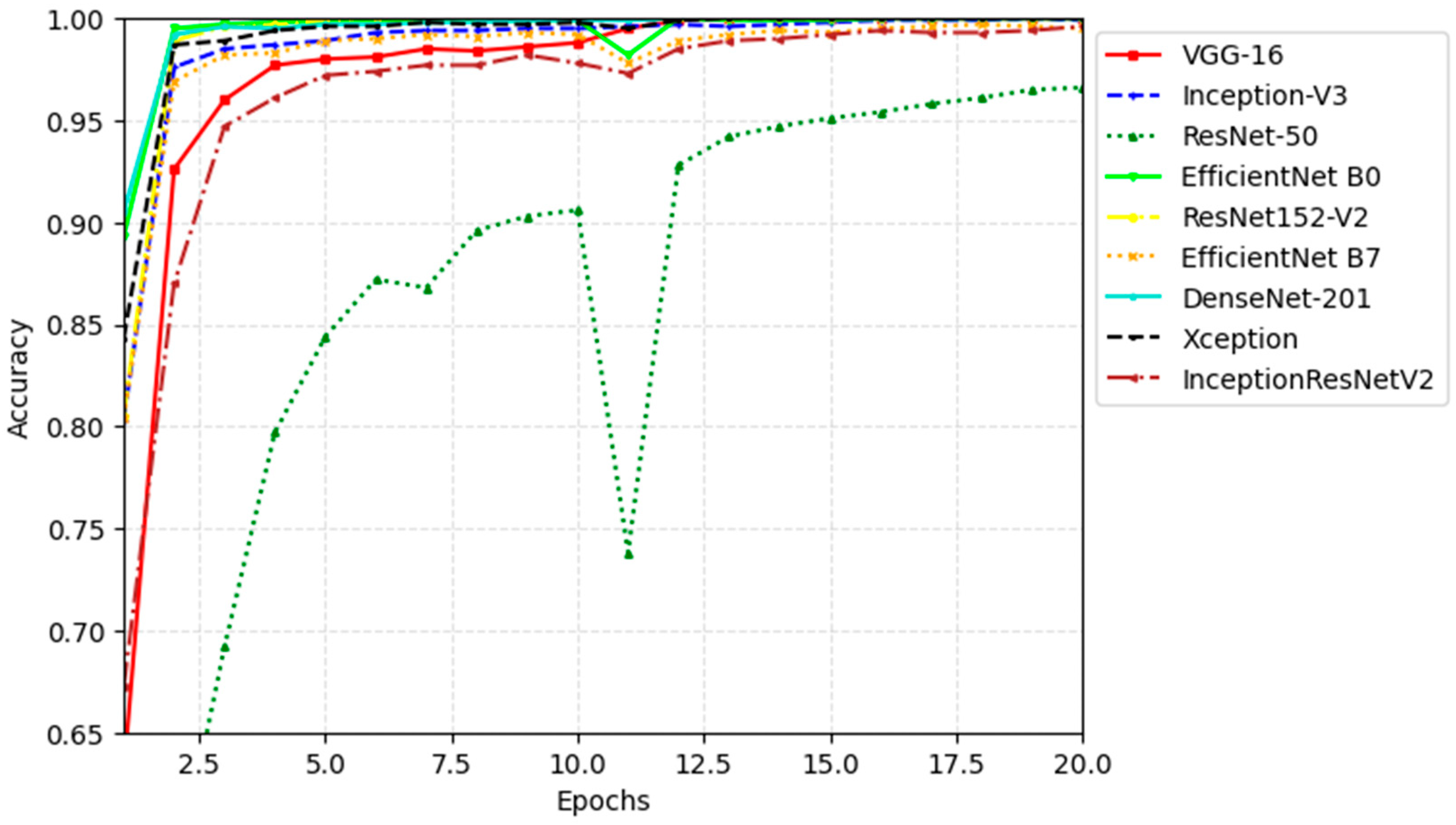
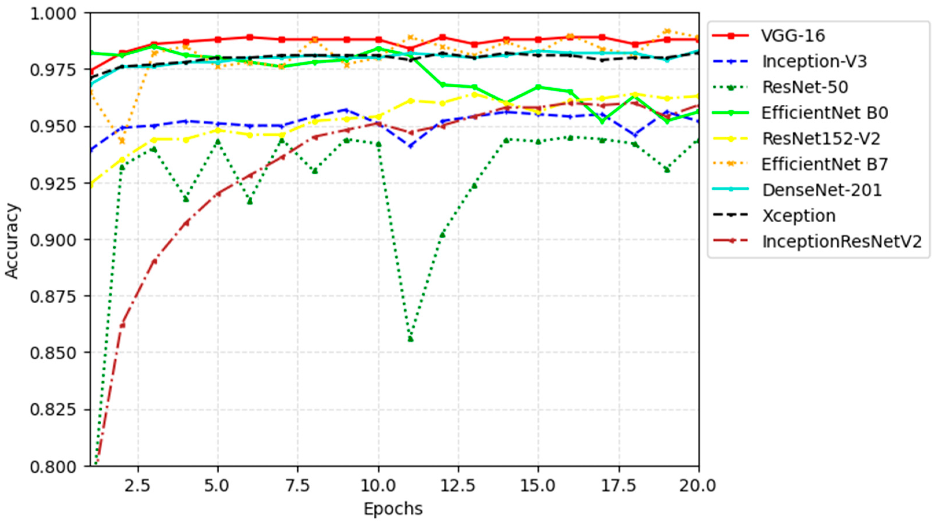
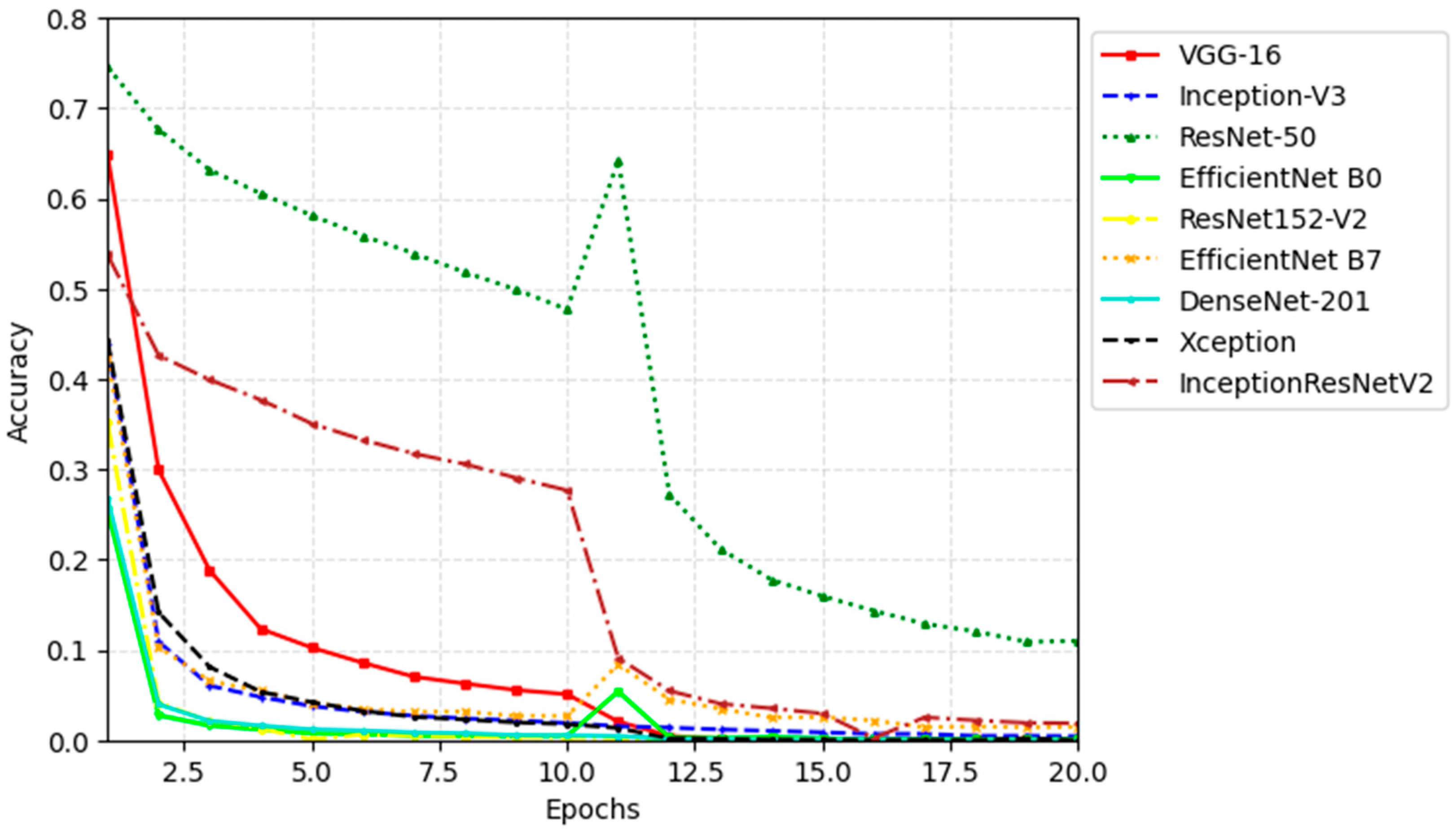
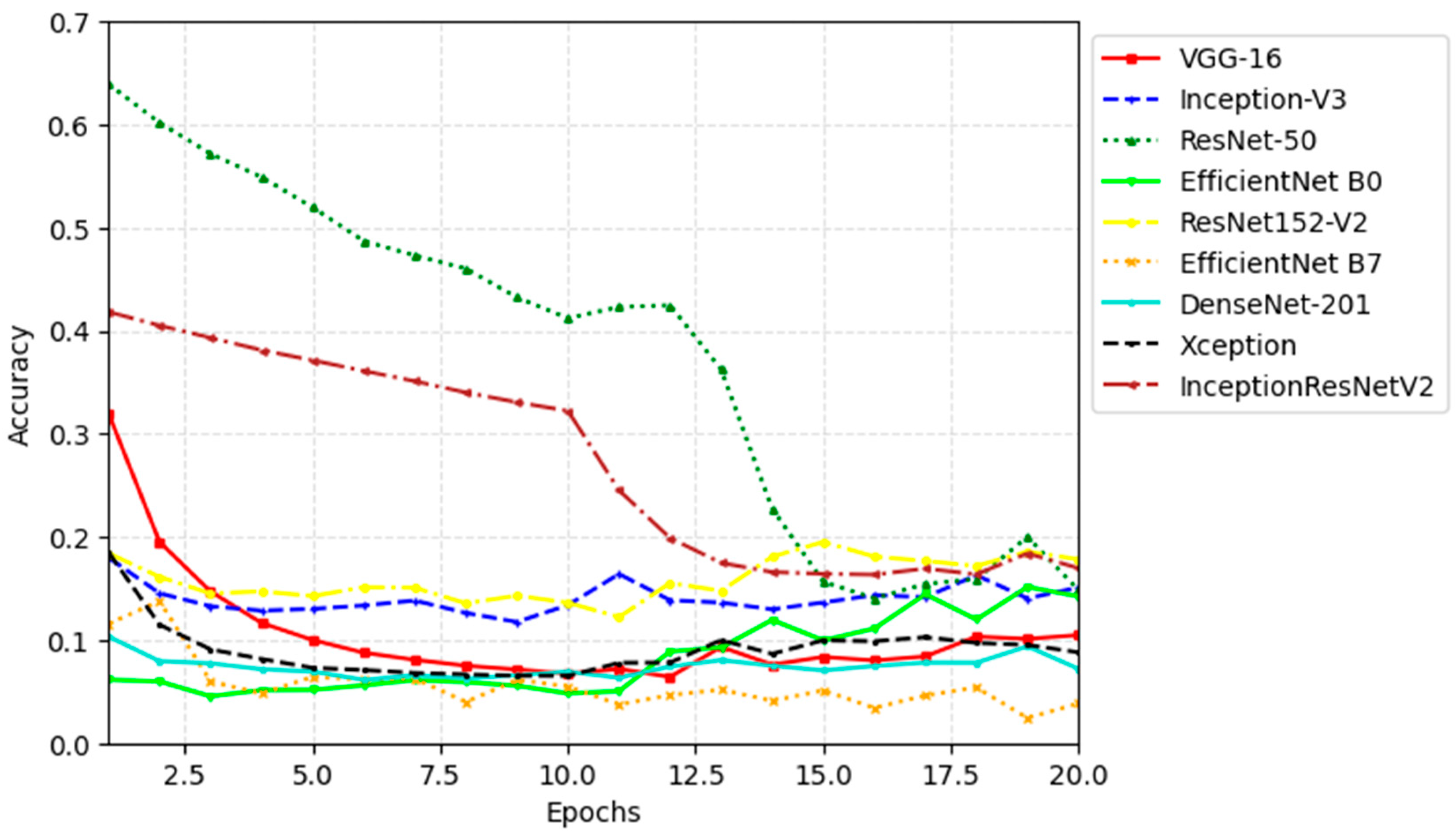
Figure 8, Figure 9, Figure 10 and Figure 11 shows the model accuracy and loss graphs across 20 epochs for all pre-trained models for brightness augmentation. As observed in Figure 8 and Figure 9, the training and validation accuracy consistently increased across the 20 epochs, exceeding 95% in most cases. VGG-16, Xception, DenseNet-201, EfficientNet B7, and EfficientNet B0 showed remarkable performances that were closely followed by InceptionResNetV2, ResNet 152 V2, and Inception-V3. ResNet 50 achieved a high accuracy of 93.16% but showed major fluctuations during training and validation. The steady increase without fluctuations in the training and validation accuracies of all the pretrained models except ResNet-50 indicates effective feature learning, absence of overfitting, stable training, and ability to generalize well on the test data.
The model losses on training and validation presented in Figure 10 and Figure 11 showed a consistent decrease from epoch 1–20 for all the pre-trained models except ResNet 50 and InceptionResNet V2. The training and validation loss curves for ResNet-50 and InceptionResNetV2 models exhibited minor fluctuations between epochs 10 and 13 but ultimately converged by epoch 20 where the loss function minimized. Generally, with the exception of ResNet-50, the training pattern of all the other models showed remarkable performance that outperforms the baseline dataset even with a smaller number of image datasets. The steady increase in training and validation accuracies of all the pre-trained models, except for ResNet-50, indicates effective feature learning, the absence of overfitting, stable training, and the ability to generalize well on the test data.
The model losses on training and validation presented in Figure 10 and Figure 11 showed a consistent decrease from epoch 1–20 for all the pre-trained models except ResNet 50 and InceptionResNet V2. The training and validation loss curves for ResNet-50 and InceptionResNetV2 models exhibited minor fluctuations between epochs 10 and 13 but ultimately converged by epoch 20 where the loss function minimized. Generally, with the exception of ResNet-50, the training pattern of all the other models showed remarkable performance that outperforms the baseline dataset even with a smaller number of image datasets.
To avoid visual clutter from the numerous image augmentation techniques, the training patterns for all augmentation types are summarized in a table rather than a figure. Table 1 indicates the presence or absence of fluctuations in accuracy and loss. To assess the training pattern of the pretrained models across the various augmentation techniques, three (3) categories were employed, which represent the level of fluctuations in accuracy and loss plots. No fluctuations (NF) represents a smooth training curve where models’ accuracy consistently increases and their loss consistently decreases without significant fluctuations. Minor fluctuations (MNF) represent training curves with minimal and relatively small fluctuations in the accuracy and loss curves. Major fluctuations (MJF) denote training curves with turbulent and substantial fluctuations in the model accuracy and loss curves, indicating a less stable training process. Several pretrained models, including VGG-16, InceptionResNetV2, Xception, and DenseNet-201, generally exhibited stable behavior during training with minimal fluctuations. Furthermore, the augmentation techniques showed no significant disruptions to the stability of these models during the training phase.

4. Discussion

4.1. Proposed Architecture of the Custom-Built Model

The design of the custom-built model involved a two-stage process. The first stage focused on hyper-parameter optimization, which was executed through multiple iterative experiments. The mini-batch size and learning rate were subject to variation in the initial stage with the aim of minimizing the model’s loss function while enhancing its evaluation metrics and minimizing both training and inference times. The second stage focused on optimizing crucial model parameters, such as the number of convolutional layers, optimizers, and kernel sizes, while preserving the best results achieved from the first stage. The results of the iterative process of the first stage are presented in Table 2. It is observed that the combination of a batch size of 128 and a learning rate of 10−5 yielded the best performance metrics (accuracy, precision, F1-score, and recall) while minimizing training and inference times, whereas the learning rates 10−1 and 10−2 performed worst, irrespective of the batch size.
The iterative process to determine the optimum number of convolutional layers was conducted by fixing the batch size and learning rate at 128 and 10−5, respectively, while varying the number of convolutional layers as shown in Table 3. The experimental results revealed that the model architecture utilizing exactly three convolutional layers achieved the highest performance across all evaluation metrics. To determine the best optimizer among Adam, RMSProp, and Adagrad for the model architecture with three convolutional layers, trained with a batch-size of 128 and learning rate of 10−5, an ablation experiment was conducted, and the results are presented in Table 4 and Table 5. The model architecture achieved its best performance when utilizing the Adam optimizer, a 3 × 3 kernel size, the categorical cross-entropy as the loss function, rectilinear units (RELU) as the activation function (hidden layer), and softmax as the activation function for the output layer.

4.2. Performance of Custom Model on Baseline and Augmented Datasets

The evaluation metrics of the custom-built model on the baseline and augmented datasets are presented in Table 6. Largely, the custom-built model, having all metrics higher than 97%, performed better on the base-graded line dataset than the augmented dataset. These high-performance metrics are indicative of the model’s ability to accurately identify cracks. The model’s performance on the augmented dataset varies with the augmentation technique applied. As can be seen from Table 6, the addition of noise to the training dataset led to a decrease in the model performance compared to the baseline dataset. For instance, precision, recall, accuracy, and F1 score reduced by 10.3%, 5.5%, 6.21%, and 5.5%, respectively, compared with the baseline datasets. The use of brightness augmentation resulted in a similar reduction in model performance as noise. The addition of extreme values of noise and brightness are capable of significantly reducing model performance. Blur and rotation caused a minor reduction in model performance compared to noise and brightness, even achieving higher recall values (98.96% and 99.04% for blur and rotation, respectively) than the baseline dataset. Shear augmentation had the least effect on model performance, producing metrics that are similar to those from the baseline datasets. In essence, shear augmentation neither significantly improved nor degraded model learning ability. Overall, some data augmentation techniques are reliable means of artificially increasing data sizes where there is a limited amount of data for training a CNN model for optimum performance. Results showed that rotation and shear are highly reliable data augmentation techniques capable of producing evaluation metrics that are comparable with those of the baseline (unaugmented) dataset.
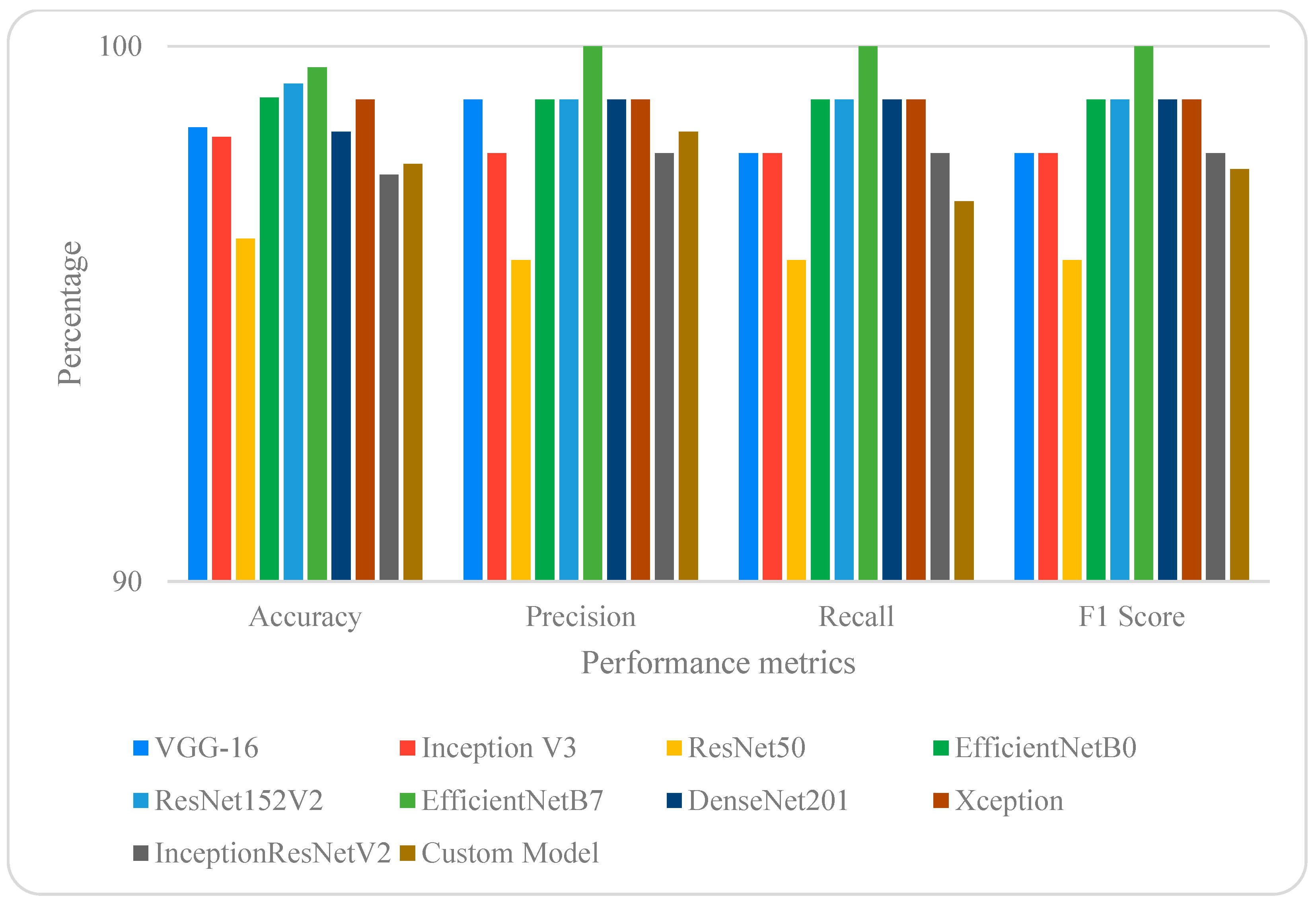
In order to evaluate the performance of the custom model, it was compared against some existing state-of-the-art (SOTA) models on the baseline datasets, and the results presented in Figure 12. Figure 12 showed that EfficientNet-B7 outperformed all models, achieving a 99.6% accuracy and 100% in recall, precision, and F1 score. Also, Xception, EfficientNet-B0, and DenseNet followed closely, achieving 99% on all evaluation metrics. The experimental results demonstrate that ResNet-50 model achieves a prediction accuracy of 96.4%, precision of 96.0%, with a recall of 96.0%, and an F1 score of 96.0%. The high metrics achieved by these models underscores their accuracy and effectiveness in crack detection. The custom-built model achieved an accuracy of 97.8%, precision of 98.4%, recall of 97.1%, and F1 score of 97.7%. The high-performance metrics of the custom-built model fell short of those of all state-of-the-art models except ResNet50.

4.3. Evaluation of the Effect of Data Augmentation on Performance of Pre-Trained Models

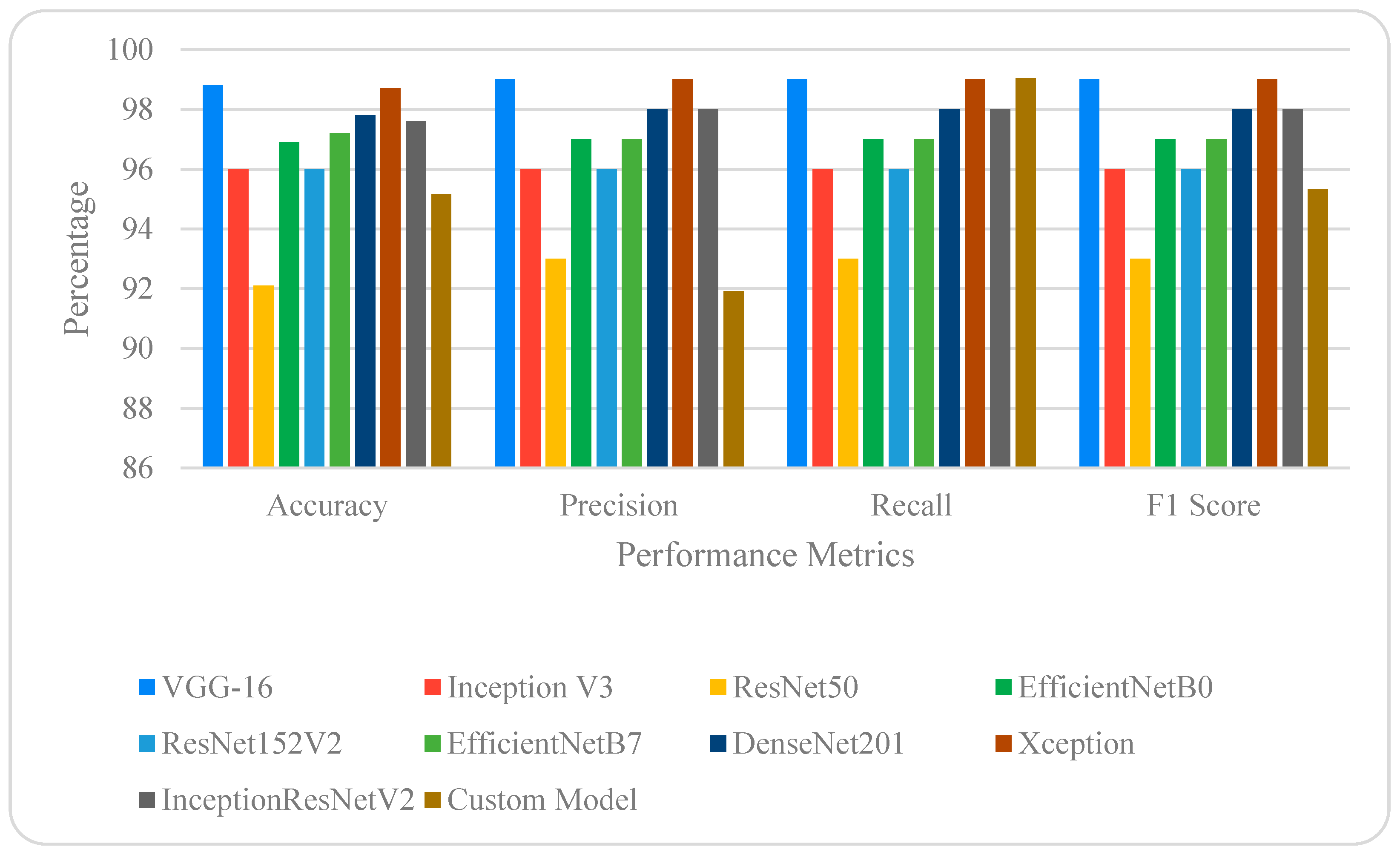
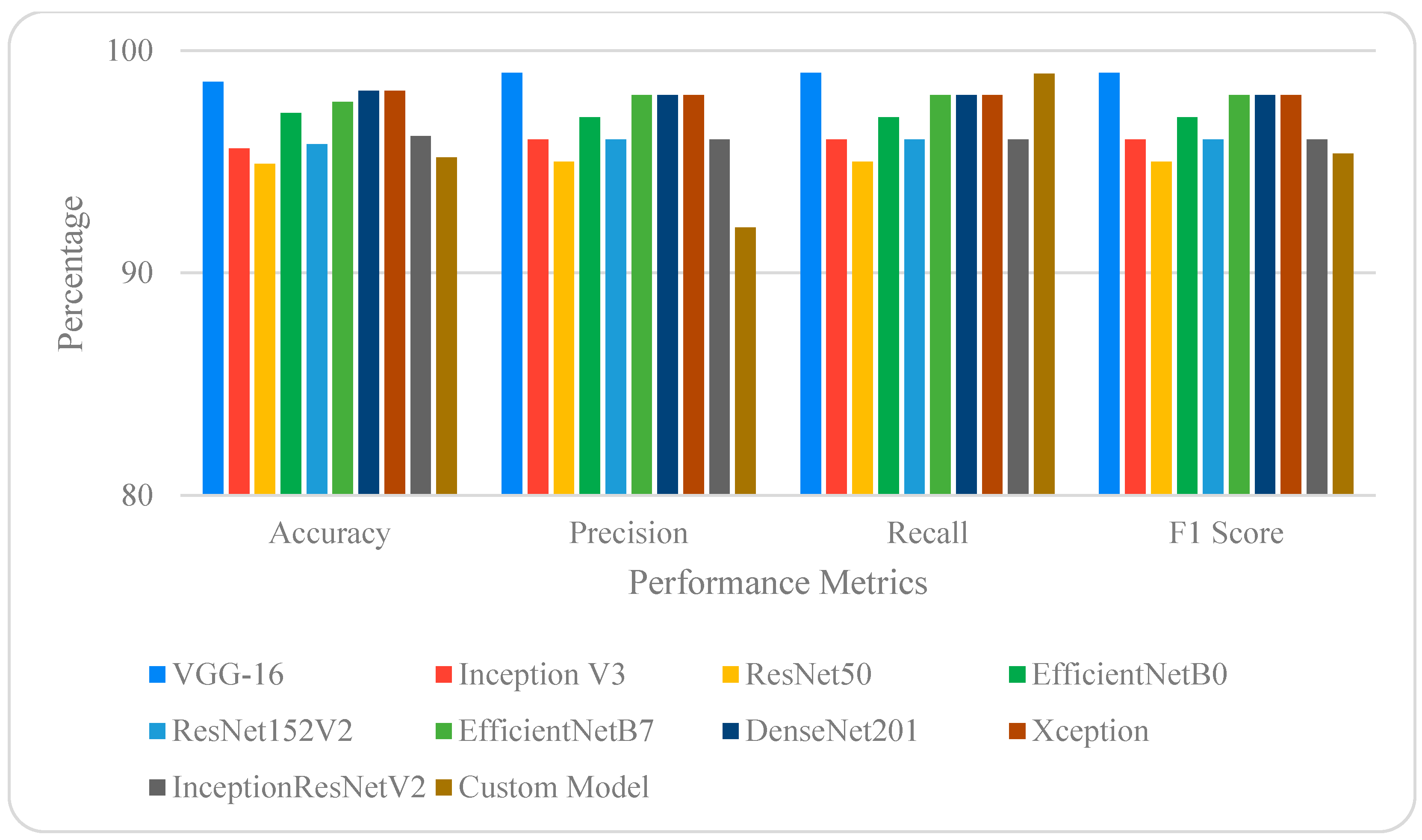
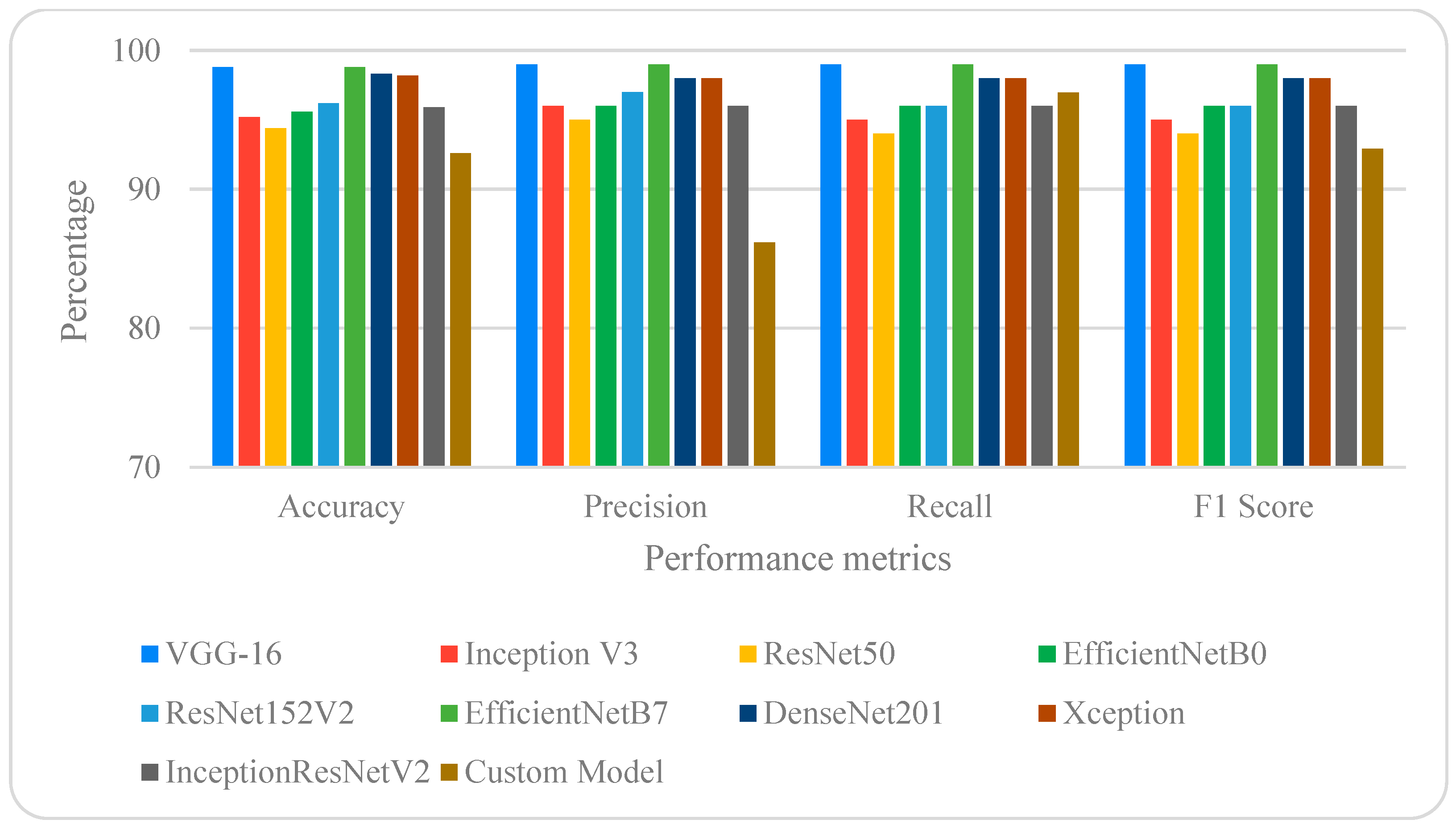
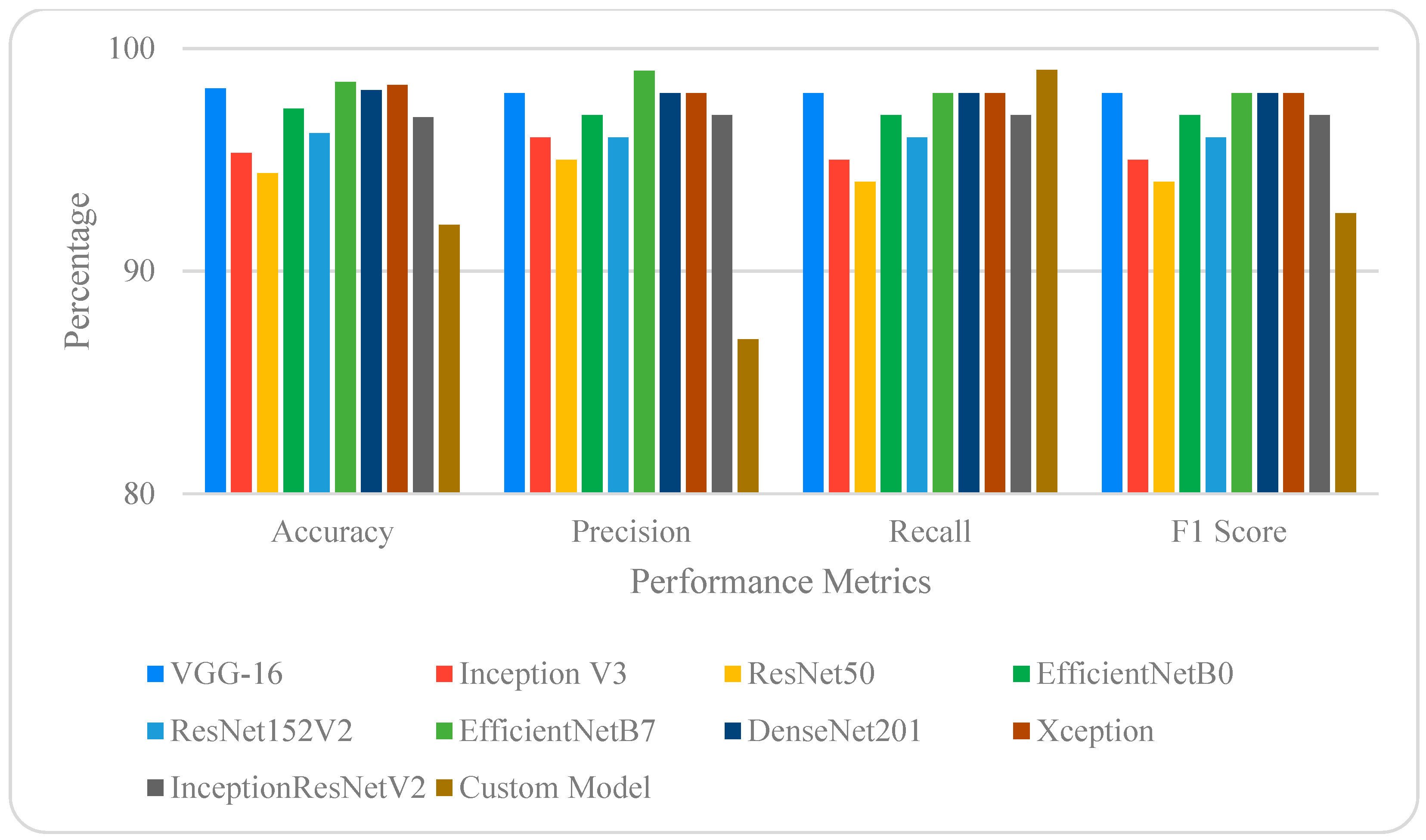
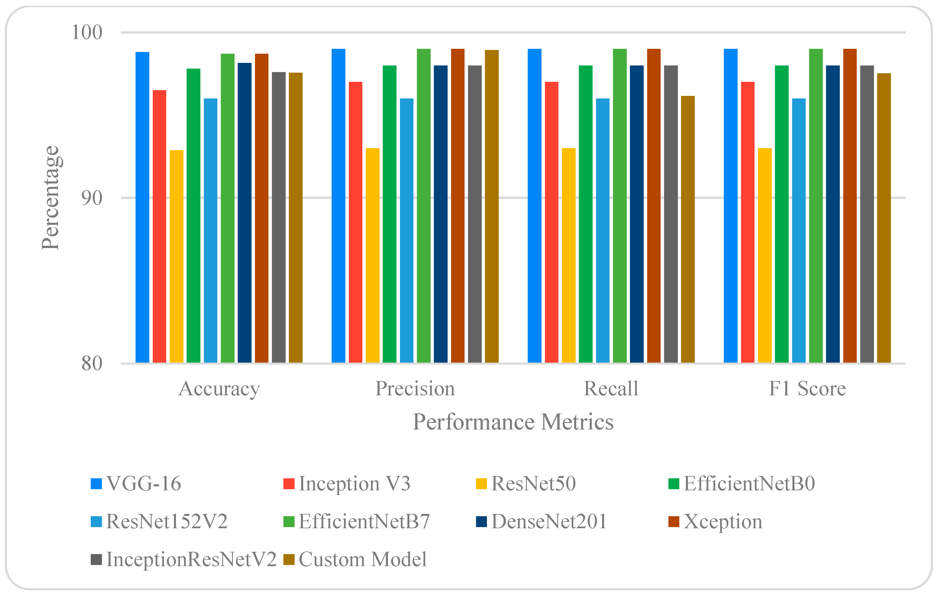
This study applies five (5) data augmentation techniques to improve the variability in the training dataset and consequently improve models’ ability to effectively learn and generalize on unseen data. The augmentation techniques include image rotation, shear, brightness, blur, and noise addition. Figure 13, Figure 14, Figure 15, Figure 16 and Figure 17 presents the performance metrics of all models across the data augmentation techniques. It can be seen from Figure 13 that VGG-16 is the best performing model followed by Xception and DenseNet-201 in descending order when image rotation augmentation was applied. When compared to the baseline model, three performance categories were observed: improvement, reduction, and no change. VGG-16 and ResNet-50 showed improvement, while Inception V3, EfficientNet-B0, EfficientNet-B7, ResNet152V2, DensNet-201, Xception, and the custom model showed reductions in performance compared with the baseline dataset. InceptionResNetV2 presented exactly the same results with the output of the baseline. In most cases, the reduction in performance metrics did not exceed 2%. In essence, image rotation augmentation increased the training dataset and improved generalization, while only leading to a minor decrease ( 2%) in the performance metrics when trained on pretrained models. This suggests that the pretrained model already offers significant level of feature extraction, thereby minimizing the impact of rotations. Conversely, rotation decreased some performance metrics by as much as 7% when trained on the custom model.
As shown in Figure 14, VGG-16 outperformed all other models on blur augmentation with the highest accuracy of 98.6%, precision of 99%, recall of 99%, and F-score of 99%. This performance is followed by Xception, DenseNet-201, EfficientNet-B7, and EfficientNet-B0, all having evaluation metrics > 97%. This indicates that image blurring had no effect on the performance of these pretrained models. However, the custom-built model and pre-trained ResNet-50 produced the lowest performances on blur augmentation, with precision decreasing by 6% compared with the performance of the baseline dataset. This suggests that blurring the images reduces the chance of a correct positive class identification, leading to an increase in the false negative rate.
Similarly, experimental results on brightness augmentation shown in Figure 15 revealed that VGG-16 and EfficientNet-B7 were the best performers, achieving 99% on accuracy, recall, precision, and F1-score. Meanwhile, compared to all pretrained models on brightness augmentation, the custom-built model had the lowest performance, achieving an accuracy of 92.6%, precision of 86.18%, recall of 96.96%, and F-score of 92.91%. The findings from noise and shear augmentation techniques shown in Figure 16 and Figure 17 indicates that VGG-16 model performed slightly better than Xception, DenseNet-201, EfficientNet-B7, and EfficientNet-B0. ResNet-50 and the custom-built model performed lowest for shear and noise augmentation, respectively.
The study results consistently showed that VGG-16, Xception, DenseNet-201, EfficientNet-B7, and EfficientNet-B0 were the best performing models across all data augmentation techniques. The consistently high performance metrics derived from VGG-16 originates from a combination of their deep architecture (16 layers) and deployment of small kernel 3 × 3 filters, enabling effective learning of complex features, leading to improved accuracy in image classification tasks [36,37,38]. The high successes of the EfficientNet (B0–B7) family of CNNs in image classification tasks is mainly due their ability to optimize network depth, width, and resolution simultaneously using a compound scaling method [31,39,40].
The sensitivity of test models to noise and illumination variations can be explained by the architectural features and training exposure. Models with shallower depth or fewer connections between layers tend to rely more on edge and fine texture signals for crack detection. Noise distorts this signal by introducing artificial pixel-level variations. This obscures crack boundaries and increases the likelihood of false negatives. Meanwhile, illumination variations alter the pixel intensity distribution and contrast between cracked regions and the background. Models trained on images with varied lighting conditions may have reduced generalization ability. In contrast, deeper and more densely connected architectures such as DenseNet-201 and Xception are more robust. These models reuse multi-path features, allowing them to preserve structural information even when low-level features are degraded. Pretrained models also benefit from prior exposure to large datasets containing high variations in image quality and illumination. This reinforces their robustness to such disturbances.
From a practical perspective, high noise sensitivity implies that these models may underperform in real-world inspections. Specifically, in image acquisition environments affected by poor sensor quality, environmental dust, or UAV camera instability, these models will underperform. Similarly, light sensitivity also highlights potential challenges in outdoor inspection (sunlight, shadows, or changing artificial lighting). For field deployment, models should be pre-trained on highly diverse datasets or combined with targeted preprocessing and augmentation techniques such as histogram equalization or denoising filters.
The effectiveness and high accuracy of Xception model stems from the replacement of regular convolution with depth-wise separable convolution, also leading to fewer computational resources. More so, the Xception model is pre-trained on large image datasets, making it highly effective in image-based damage detection tasks [41,42]. DenseNet model creates a unique pattern of connecting each layer to every other layer. In essence, each subsequent layer receives input from all preceding layers and passes its own feature maps to all subsequent layers. This architecture eliminates the vanishing gradient problem, improves feature propagation, enhance feature reuse, and significantly minimize the number of parameters involved in the computations [43,44]. Inception V3 depends on parallel convolution layers, factorized convolutions, and other optimization techniques to achieve high accuracy at less computational expense on image-based classification tasks [45]. Extensive image features are effectively captured from images by combining various filter sizes and dimensionality reduction techniques without any significant increase in computational cost and a reduced error rate. These major advantages make Inception V3 highly suitable for image classification and transfer learning tasks [46,47]. The main advantage of ResNet model architectures is their ability to effectively train deep neural networks through the use of residual connections, otherwise known as skip connections. The skip connections bypass one or more layers, permitting the input to be added to the output within a block of layers. ResNet improves the efficiency of information dissemination, leading to improved accuracy, easier optimization, and an eventual solution to the vanishing gradient problem [48,49].

4.4. Model Performances on Real-World Noise Datasets

To evaluate the reliability of the noise augmentation phase of the study, both the custom-built and pre-trained CNN models were run on real-world images of cracked objects containing noise. The real-world noise image data was adopted from Zhou [48] and contains 984 positive images of cracks with diverse forms of real noise (Figure 18). Table 7 presents a comparison of various evaluation metrics for machine learning models, including accuracy, precision, recall, F1-score, and both training and inference times. In most cases, a slight decrease in the evaluation metrics was observed when the real-world noise data was used compared with the augmented dataset. For instance, the accuracy, precision, and F1-score of the high-performing VGG-16 slightly decreased from 98.2%, 98%, and 98% to 97.2%, 95%, and 97%, respectively, when real-world noise data was used.
There was a slight improvement in the recall from 98% to 100%. A similar trend was observed for DenseNet-201, Xception, and ResNet152V2. The above-mentioned models showed some degree of consistency on both augmented and real-world noise data and therefore validated the reliability of the noise augmentation preprocessing technique. However, Inception V3, ResNet50, InceptionResNetV2, EfficientNetB7, and EfficientNetB0 exhibited significant decreases in evaluation metrics.

4.5. Confusion Matrices

While the evaluation metrics like accuracy, precision, recall, and F1 score are useful tools for assessing a model’s performance, a confusion matrix offers a more reliable visualization of its efficiency on unseen data. The confusion matrix helps in understanding how well the CNN model distinguishes between the different classes on the test (unseen) data in image-based classification tasks by showing the number of correctly and incorrectly classified instances. The true positives (TP), false negatives (FN), true negatives (TN), and false positives (FP) are extracted from a large number of confusion matrices and presented in Table 8, Table 9, Table 10, Table 11, Table 12 and Table 13.
The outputs from the confusion metrics of the baseline datasets when trained with the custom built and pretrained models are compared in Table 8. EfficientNet-B7 outclassed all other models, achieving a TP = 622, FP = 3, FN = 2, and TN = 623. ResNet152V2 was slightly behind EfficientNet-B7 with TP = 618, FP = 7, FN = 2, and TN= 623. Although Xception, DenseNet-201, Inception-V3, and EfficientNetB0 had more misclassifications, their performance on the unseen dataset was equally good. Interestingly, the consistently high-performing VGG-16 misclassified 19 uncracked images as cracked images, while accurately classifying all 600 uncracked images. Furthermore, misclassifying a small amount of uncracked images as cracked images is common in image-based classifications, especially when dealing with subtle difference in surface conditions.
The confusion matrices for rotation augmentation are presented in Table 9. As observed from the values, VGG-16 has 1248 true positives (TP) out of 1250 positive instances (cracks) and 1222 true negatives (TN) out of 1250 negative instances (no cracks). These results translate to true positive rate (TPR) and true negative rate (TNR) of 99.84% and 97.76%, respectively. High values of TPR and TNR indicates a strong ability of the model to correctly classify both positive (cracked) and negative (uncracked) surfaces in the dataset. Furthermore, the confusion matrices demonstrate the superiority of the pretrained VGG-16 model over the other models, including the custom-built model in a crack identification and classification task. A noteworthy observation from Table 9 is the relatively high number of correct negative (uncracked) classifications across all the models. This indicates that the models were favorable towards detecting uncracked surfaces. When compared to the baseline classification studies, image rotation effectively increases image data size and improves the generalization capability of both pretrained and custom-built models.
The experimental results for blurring augmentation in Table 10 revealed that VGG-16 performed better, correctly classifying 1219 cracked surfaces out of a possible 1250, misclassifying 31 cracked images as uncracked images. This translates to a true positive rate of 97.7%, suggesting that when VGG-16 classifies an image as cracked, then it is highly likely to be a crack. This is a strong indication of the superiority and robustness of VGG-16 whose identification capabilities are not affected synthetically adding blur images to the training datasets. DenseNet-201 and Xception models performed well, achieving a true positive rate of 97.3% and 96.9%, respectively. Conversely, Inception V3, ResNet152V2, and the custom-built model were most affected by image-blurring augmentation, achieving a reduced true positive rate of 93.2%, 91.8%, and 87.8%, respectively. Similar to the rotation augmentation, all models were generally better at predicting uncracked images than cracked images. This suggests that even with image-blurring, the models are capable of classifying uncracked images to a high degree of accuracy.
The confusion matrices of image brightness augmentation presented in Table 11 showed that EfficientNetB7 outclassed all the others with a true positive rate (TPR) and true negative rate (TNR) of 97.8% and 100%, respectively. Other high performing models are VGG-16, DenseNet201, and Xception, with all TPRs and TNRs greater than 95%. The custom-built model had the least performance for TPR (87.38%) and appeared to be significantly affected by the image brightness augmentation technique. Overall, the results suggest that the brightness augmentation technique enhanced the model training and generalization ability of most pretrained models.
The result of image noise augmentation, presented in Table 12 revealed that EfficientNet-B7 (TPR = 97.4%), Xception (TPR = 96.8%), VGG-16 (TPR = 96.6%), and DenseNet201 (TPR = 96.3%) are the best performing models. The custom-built model and ResNet-50 are the worst performing models, as the results suggest that they are highly susceptible to noise in the training dataset. For the baseline dataset, the best performing EfficientNet-B7 and custom-built models achieved TPRs of 99.5% and 98.4%. These figures dropped to 97.4% and 85.1%, respectively, after noise augmentation, suggesting that the pre-trained model was more robust to the added noise.
Shear performance of the confusion matrices for all pretrained and custom-built models are presented in Table 13. Interestingly, the custom-built model had the highest TPR of 95.15% and the lowest TNR of 96.2%, indicating a very good capability to accurately identify cracks and uncracked surfaces. Generally, shear augmentation produced more pretrained models having TP > 1200 out of 1250 than any augmentation technique applied. This suggests that shear augmentation enhanced model performance during the training, validation, and testing phases. ResNet-50, with 153 false positives, had the worst misclassification of all the pretrained models.

4.6. Comparison of Model Complexities and Computational Efficiency

Models which achieve remarkable accuracy and precision must be evaluated on critical factors such as computational cost, model complexities, and efficient utilization of resources. This comprehensive evaluation is crucial to ensure model suitability for deployments on lightweight devices, unmanned aerial vehicles (UAVs) or other platforms with limited hardware resources. The evaluating metrics for lightweight models include floating-point operations (FLOPs), number of parameters involved in the computations, number of parameters, model size, and inference/training time [3,4]. While FLOPs measure the computational cost of a model during training, the number of parameters relates to the model’s complexity and capacity. Model size and training times indicate memory footprint and time required by the model for effective training, respectively. These parameters are presented in Table 14. As observed in Table 14, InceptionResNet has the highest number of deep layers, 449, and is closely followed by EfficientNetB7 and DenseNet 201 with 438 and 402 deep layers, respectively. VGG-16 has the maximum FLOPs of 16G, followed by InceptionResNet and ResNet152V2 with 15.1G and 11G, respectively. VGG-16 has the highest number of parameters, which is more than twice as many of ResNet152V2 and EfficientNet B7, indicating significantly high computational cost and memory requirement, making it unsuitable for resource-constrained devices or edge computing environments. Meanwhile, VGG has the longest training time of all the pre-trained CNN models. In contrast to most pre-trained CNN models, the proposed model had the lowest FLOP, which is less than 2% of the FLOP required by the high-performing VGG-16. Also, among all the models, the proposed custom model had the least number of parameters, smallest model size, and shortest running time. These metrics indicate the proposed model is lightweight, requires significantly less memory, and is fast and computationally efficient, making it an innovative solution suitable for edge computing environments deployable on resource constrained devices such as UAVs [51]. Although the accuracy of the custom-built CNN is slightly lower than that of outstanding VGG-16 and a few other pre-trained models across all augmentation techniques, its great advantage is the trade-off it offers between accuracy and other critical factors such as computational expense, speed, and memory footprint.

5. Implication of the Study

This study examined the impact of five data augmentation techniques, shear, rotation, noise, blur, and brightness, on the performance of a custom-built convolutional neural network (CNN) and nine pre-trained CNN models. To demonstrate the practical benefit of this approach, the results were compared to a previous study by Omoebamije et al. [2], where a lightweight CNN model was trained from scratch on a large, generic dataset of crack images. In that earlier study, 30,000 images were used for training and 2500 for testing. Although the model achieved impressive results (99.0% accuracy, 98.8% precision, 99.3% recall, and 99.0% F1-score), the process required over 30 days of data acquisition and preprocessing by three personnel, totaling approximately 32,500 manually prepared images.
In contrast, this current study demonstrated that comparable performance can be achieved using far fewer images when data augmentation and transfer learning are effectively applied. The custom-built CNN, trained on just 15,000 images (half the original dataset), still achieved 97.8% accuracy, 98.4% precision, 97.1% recall, and 97.1% F1-score. More remarkably, using only 3750 augmented images per experiment, several pre-trained models including VGG-16, EfficientNet-B7, EfficientNet-B0, DenseNet-201, and Xception, produced results that not only matched but, in some cases, surpassed the metrics achieved in the original large-data study. For instance, under brightness augmentation alone, these models outperformed the previous benchmarks across multiple evaluation metrics.
These findings highlight the effectiveness of combining state-of-the-art pretrained CNN models with data augmentation techniques on smaller image datasets to reduce the need for large-scale image datasets. This approach significantly lowers the labor and time costs associated with manual data collection and preprocessing. Moreover, the study builds on and corroborates prior findings [10,52,53] by using the traditional augmentation technique in a distinct manner with numerous state-of-the-art pretrained models.

6. Conclusions

This study investigated the effect of five distinct data augmentation techniques, shear, rotation, noise, blur, and brightness, on the crack detection performance of a custom-built convolutional neural network (CNN) and nine pre-trained CNN models. Each model was trained on both a baseline dataset (unaugmented) and separately augmented datasets. The key findings are summarized as follows:
  • The custom CNN model achieved over 97% in accuracy, precision, recall, and F1-score on the baseline dataset. However, its performance declined when trained on augmented data, especially with noise and brightness, which reduced precision to 86.94% and 89.18%, respectively. Shear, rotation, and blur had minimal impact.
  • Among all models, EfficientNet-B7 outperformed the rest, achieving 99.6% accuracy and perfect scores (100%) across all metrics on the baseline dataset. Other strong performers included Xception, EfficientNet-B0, and DenseNet-201. Except for ResNet50, all pre-trained models surpassed the custom CNN.
  • Across all augmentation techniques, VGG-16, Xception, EfficientNet-B0, EfficientNet-B7, and DenseNet-201 consistently ranked highest in performance. Notably, VGG-16 maintained 99% across all key metrics regardless of the augmentation type.
  • Confusion matrices revealed that these top models produced high true positive and true negative counts with minimal misclassifications, confirming their reliability and robustness in real-world crack detection tasks.
  • The results demonstrate that applying targeted augmentation techniques in conjunction with pre-trained CNN models can deliver high accuracy, even when training data is limited. This mitigates the need for large-scale datasets in crack detection applications.
Contributions of this study include: (1) a targeted evaluation of five augmentation strategies on a lightweight custom CNN model; (2) a comparative analysis of nine state-of-the-art pre-trained CNNs trained on individually augmented datasets; and (3) a performance benchmark relative to prior work using large datasets.
Future work should explore the combined effect of multiple augmentation techniques and assess other lightweight or real-time architectures such as MobileNet, DarkNet, ShuffleNet, AlexNet, and YOLO to further expand the understanding of model suitability under data-constrained conditions. Also, more recent CNN architecture such as ConvNeXt V2, EfficientNetV2, and SWIM transformers should be considered to investigate the effect of data augmentation on model performance.

Author Contributions

Conceptualization, T.M.O. and O.O.; methodology, T.M.O. and B.A.; software, T.M.O. and O.O.; validation, all authors; investigation, T.M.O. and O.O.; formal analysis, T.M.O., Z.M.O., and T.Q.M.; resources, B.A. and T.M.O.; data curation, O.O. and Z.M.O.; writing—original draft preparation, all authors; writing—review and editing, all authors; visualization, O.O. and T.M.O.; supervision, J.C.M. and J.T. All authors have read and agreed to the published version of the manuscript.

Funding

This research was fully funded by the institutional based research (IBR) of Tertiary Education Fund issued to the Nigerian Army University Biu with reference: TETF/DR&D/CE/UNIV/NAUBIU/IBR/2024/VOL.1.

Institutional Review Board Statement

Not applicable.

Informed Consent Statement

Not applicable.

Data Availability Statement

The data and codes presented in this study are available on request from the corresponding author.

Acknowledgments

The authors are thankful for the support from the Federal Ministry of Education Nigeria and the Nigerian Army University Biu.

Conflicts of Interest

The authors declare no conflicts of interest.

Abbreviations

The following abbreviations are used in this manuscript:
CNNConvolutional neural network
VIVisual inspection
AIArtificial intelligence
DLDeep learning
NLPNatural language processing
CLAHEContrast limited adaptive histogram equalization
UAVUnmanned aerial vehicle
GANGenerative adversarial networks
SMOTESynthetic minority oversampling technique
ROCReceiver operating characteristics
PRPrecision-recall
NFNo significant fluctuations
MNFMinor and relatively small fluctuations
MJFMajor fluctuations
TPTrue positive
TNTrue negative
FPFalse positive
FNFalse negative
TPRTrue positive rate
TNRTrue negative rate

References

  1. Abubakr, M.; Rady, M.; Bedran, K.; Mahfouz, S. Application of deep learning in damage classification of reinforced concrete bridges. Ain Shams Eng. J. 2024, 15, 102297. [Google Scholar] [CrossRef]
  2. Omoebamije, O.; Omoniyi, T.M.; Musa, A.; Duna, S. An improved deep learning convolutional neural network for crack detection based on UAV images. Innov. Infrastruct. Solut. 2023, 8, 236. [Google Scholar] [CrossRef]
  3. Dorafshan, S.; Thomas, R.J.; Maguire, M. Comparison of deep convolutional neural networks and edge detectors for image-based crack detection in concrete. Constr. Build. Mater. 2018, 186, 1031–1045. [Google Scholar] [CrossRef]
  4. Mohammadzadeh, M.; Kremer, G.E.O.; Olafsson, S.; Kremer, P.A. AI-Driven crack detection for remanufacturing cylinder heads using deep learning and Engineering-Informed data augmentation. Automation 2024, 5, 578–596. [Google Scholar] [CrossRef]
  5. Minh, T.; Van, T.N.; Nguyen, H.X.; Nguyễn, Q. Enhancing the Structural Health Monitoring (SHM) through data reconstruction: Integrating 1D convolutional neural networks (1DCNN) with bidirectional long short-term memory networks (Bi-LSTM). Eng. Struct. 2025, 340, 120767. [Google Scholar] [CrossRef]
  6. Minh, T.; Matos, J.C.; Sousa, H.S.; Ngoc, S.D.; Van, T.N.; Nguyen, H.X.; Nguyen, Q. Data reconstruction leverages one-dimensional Convolutional Neural Networks (1DCNN) combined with Long Short-Term Memory (LSTM) networks for Structural Health Monitoring (SHM). Measurement 2025, 253, 117810. [Google Scholar] [CrossRef]
  7. Thompson, N.; Fleming, M.; Tang, B.J.; Pastwa, A.M.; Borge, N.; Goehring, B.C.; Das, S. A model for estimating the economic costs of computer vision systems that use deep learning. Proc. AAAI Conf. Artif. Intell. 2024, 38, 23012–23018. [Google Scholar] [CrossRef]
  8. Ying, X. An Overview of Overfitting and its Solutions. J. Phys. Conf. Ser. 2019, 1168, 022022. [Google Scholar] [CrossRef]
  9. Pan, S.J.; Yang, Q. A survey on transfer learning. IEEE Trans. Knowl. Data Eng. 2009, 22, 1345–1359. [Google Scholar] [CrossRef]
  10. Shorten, C.; Khoshgoftaar, T.M. A survey on Image Data Augmentation for Deep Learning. J. Big Data 2019, 6, 60. [Google Scholar] [CrossRef]
  11. Wen, Q.; Gao, J.; Sun, L.; Xu, H.; Lv, J.; Song, X. Time series data augmentation for deep learning: A survey. arXiv 2021, arXiv:2002.12478. [Google Scholar]
  12. Feng, S.Y.; Gangal, V.; Wei, J.; Chandar, S.; Vosoughi, S.; Mitamura, T.; Hovy, E. A survey of Data Augmentation Approaches for NLP. arXiv 2021, arXiv:2105.03075. [Google Scholar] [CrossRef]
  13. Ko, T.; Peddinti, V.; Povey, D.; Khudanpur, S. Audio augmentation for speech recognition. Proc. Interspeech 2015, 2015, 3586–3589. [Google Scholar] [CrossRef]
  14. Gu, S.; Pednekar, M.; Slater, R. Improve Image Classification Using Data Augmentation and Neural Network. SMU Data Sci. Rev. 2019, 2, 1. [Google Scholar]
  15. Kim, B.; Cho, S. Automated Vision-Based detection of cracks on concrete surfaces using a deep learning technique. Sensors 2018, 18, 3452. [Google Scholar] [CrossRef]
  16. Xu, M.; Yoon, S.; Fuentes, A.; Park, D.S. A comprehensive survey of image augmentation techniques for deep learning. Pattern Recognit. 2023, 137, 109347. [Google Scholar] [CrossRef]
  17. Osman, M.K.; Mohammad, Z.E.A.; Idris, M.; Ahmad, K.A.; Muhamed, Y.N.A.; Ibrahim, A.; Hasnur, R.A.; Bahri, I. Pavement Crack Classification using Deep Convolutional Neural Network. J. Mech. Eng. 2021, 1, 227–244. [Google Scholar]
  18. Nguyen, C.L.; Nguyen, A.; Brown, J.; Byrne, T.; Ngo, B.T.; Luong, C.X. Optimising Concrete Crack Detection: A Study of Transfer Learning with Application on Nvidia Jetson Nano. Sensors 2024, 24, 7818. [Google Scholar] [CrossRef] [PubMed]
  19. Zhang, Q.; Zhu, Y.; Yang, M.; Jin, G.; Zhu, Y.; Lu, Y.; Zou, Y.; Chen, Q. An improved sample selection framework for learning with noisy labels. PLoS ONE 2024, 19, e0309841. [Google Scholar] [CrossRef]
  20. Zhang, Q.; Zhu, Y.; Cordeiro, F.R.; Chen, Q. A progressive sample selection framework with contrastive loss designed for noisy labels. Pattern Recognit. 2025, 16, 111284. [Google Scholar] [CrossRef]
  21. Kim, J.; Seon, S.; Kim, S.; Sun, Y.; Lee, S.; Kim, J.; Hwang, B.; Kim, J. Generative AI-Driven Data Augmentation for Crack Detection in Physical Structures. Electronics 2024, 13, 3905. [Google Scholar] [CrossRef]
  22. Zhou, Z.; Zhang, J.; Gong, C.; Wu, W. Automatic tunnel lining crack detection via deep learning with generative adversarial network-based data augmentation. Undergr. Space 2022, 9, 140–154. [Google Scholar] [CrossRef]
  23. Choi, S.M.; Cha, H.S.; Jiang, S. Hybrid Data Augmentation for Enhanced Crack Detection in Building Construction. Buildings 2024, 14, 1929. [Google Scholar] [CrossRef]
  24. Jamshidi, M.; El-Badry, M.; Nourian, N. Improving Concrete Crack Segmentation Networks through CutMix Data Synthesis and Temporal Data Fusion. Sensors 2023, 23, 504. [Google Scholar] [CrossRef] [PubMed]
  25. Widodo, A.O.; Setiawan, B.; Indraswari, R. Machine Learning-Based intrusion detection on multi-class imbalanced dataset using SMOTE. Procedia Comput. Sci. 2024, 234, 578–583. [Google Scholar] [CrossRef]
  26. Mohammed, R.; Rawashdeh, J.; Abdullah, M. Machine Learning with Oversampling and Undersampling Techniques: Overview Study and Experimental Results. In Proceedings of the 11th International Conference on Information and Communication Systems (ICICS), Irbid, Jordan, 7–9 April 2020; pp. 243–248. [Google Scholar] [CrossRef]
  27. Walawalkar, D.; Shen, Z.; Liu, Z.; Savvides, M. Attentive CutMix: An enhanced data augmentation approach for deep learning based image classification. In Proceedings of the IEEE International Conference on Acoustics, Speech and Signal Processing (ICASSP), Barcelona, Spain, 4–8 May 2020. [Google Scholar] [CrossRef]
  28. Simonyan, K.; Zisserman, A. Very deep convolutional networks for large-scale image recognition. arXiv 2014, arXiv:1409.1556. [Google Scholar]
  29. He, K.; Zhang, X.; Ren, S.; Sun, J. Deep Residual Learning for Image Recognition. CVPR 2016, 770–778. [Google Scholar] [CrossRef]
  30. Szegedy, C.; Ioffe, S.; Vanhoucke, V.; Alemi, A. Inception-V4, Inception-ResNet and the impact of residual connections on learning. Proc. AAAI Conf. Artif. Intell. 2017, 31. [Google Scholar] [CrossRef]
  31. Tan, M.; Le, Q.V. EfficientNet: Rethinking model scaling for convolutional neural networks. arXiv 2019, arXiv:1905.11946. [Google Scholar] [CrossRef]
  32. Huang, G.; Liu, Z.; Van Der Maaten, L.; Weinberger, K.Q. Densely Connected Convolutional Networks. In Proceedings of the IEEE Conference on Computer Vision and Pattern Recognition (CVPR), Honolulu, HI, USA, 21–26 July 2017. [Google Scholar] [CrossRef]
  33. Huang, G.; Liu, Z.; Pleiss, G.; Van Der Maaten, L.; Weinberger, K.Q. Convolutional Networks with Dense Connectivity. IEEE Trans. Pattern Anal. Mach. Intell. 2019, 44, 8704–8716. [Google Scholar] [CrossRef]
  34. Chollet, F. Xception: Deep Learning with Depthwise Separable Convolutions. In Proceedings of the 30th IEEE Conference on Computer Vision and Pattern Recognition (CVPR), Honolulu, HI, USA, 21–26 July 2017; pp. 1800–1807. [Google Scholar] [CrossRef]
  35. He, K.; Zhang, X.; Ren, S.; Sun, J. Identity mappings in deep residual networks. Lecture notes in computer science. In Proceedings of the European Conference on Computer Vision, Honolulu, HI, USA, 17 September 2016; pp. 630–645. [Google Scholar] [CrossRef]
  36. Mittal, K.; Gill, K.S.; Chattopadhyay, S.; Singh, M. Innovative Solutions for solar panel maintenance: A VGG16-Based approach for early damage Detection. In Proceedings of the International Conference on Communication, Computing and Internet of Things (IC3IoT), Chennai, India, 17–18 April 2024; pp. 1–4. [Google Scholar] [CrossRef]
  37. Fan, C. Deep neural networks for automated damage classification in image-based visual data of reinforced concrete structures. Heliyon 2024, 10, e38104. [Google Scholar] [CrossRef] [PubMed]
  38. Swain, S.; Tripathy, A.K. Automatic detection of potholes using VGG-16 pre-trained network and Convolutional Neural Network. Heliyon 2024, 10, e30957. [Google Scholar] [CrossRef]
  39. Fu, R.; Cao, M.; Novák, D.; Qian, X.; Alkayem, N.F. Extended efficient convolutional neural network for concrete crack detection with illustrated merits. Autom. Constr. 2023, 156, 105098. [Google Scholar] [CrossRef]
  40. Ali, H.; Shifa, N.; Benlamri, R.; Farooque, A.A.; Yaqub, R. A fine-tuned EfficientNet-B0 convolutional neural network for accurate and efficient classification of apple leaf diseases. Sci. Rep. 2025, 15, 25732. [Google Scholar] [CrossRef]
  41. Gülmez, B. A novel deep neural network model based Xception and genetic algorithm for detection of COVID-19 from X-ray images. Ann. Oper. Res. 2022, 328, 617–641. [Google Scholar] [CrossRef] [PubMed]
  42. Joshi, S.A.; Bongale, A.M.; Olsson, P.O.; Urolagin, S.; Dharrao, D.; Bongale, A. Enhanced Pre-Trained Xception Model Transfer learned for breast cancer detection. Computation 2023, 11, 59. [Google Scholar] [CrossRef]
  43. Akgül, İ. Mobile-DenseNet: Detection of building concrete surface cracks using a new fusion technique based on deep learning. Heliyon 2023, 9, e21097. [Google Scholar] [CrossRef]
  44. Alfaz, N.; Hasnat, A.; Khan, A.; Sayom, N.; Bhowmik, A. Bridge Crack Detection Using Dense Convolutional Network (Densenet). In Proceedings of the 2nd International Conference on Computing Advancements, New York, NY, USA, 11 August 2022; pp. 509–515. [Google Scholar] [CrossRef]
  45. Ahmed, M.; Afreen, N.; Ahmed, M.; Sameer, M.; Ahamed, J. An inception V3 approach for malware classification using machine learning and transfer learning. Int. J. Intell. Netw. 2023, 4, 11–18. [Google Scholar] [CrossRef]
  46. Ehtisham, R.; Qayyum, W.; Camp, C.V.; Plevris, V.; Mir, J.; Khan, Q.Z.; Ahmad, A. Classification of defects in wooden structures using pre-trained models of convolutional neural network. Case Stud. Constr. Mater. 2023, 19, e02530. [Google Scholar] [CrossRef]
  47. Meftah, I.; Hu, J.; Asham, M.A.; Meftah, A.; Zhen, L.; Wu, R. Visual Detection of Road Cracks for Autonomous Vehicles Based on Deep Learning. Sensors 2024, 24, 1647. [Google Scholar] [CrossRef]
  48. Zhang, J.; Bao, T. An Improved ResNet-Based Algorithm for Crack Detection of Concrete Dams Using Dynamic Knowledge Distillation. Water 2023, 15, 2839. [Google Scholar] [CrossRef]
  49. Wen, L.; Xiao, Z.; Xu, X.; Liu, B. Disaster Recognition and Classification Based on Improved ResNet-50 Neural Network. Appl. Sci. 2025, 15, 5143. [Google Scholar] [CrossRef]
  50. Zhou, J.H. Noise Crack Dataset. GitHub. 2020. Available online: https://github.com/zhoujh2020/ (accessed on 10 November 2025).
  51. Zhang, R.; Jiang, H.; Wang, W.; Liu, J. Optimization Methods, Challenges, and Opportunities for Edge Inference: A Comprehensive Survey. Electronics 2025, 14, 1345. [Google Scholar] [CrossRef]
  52. Alomar, K.; Aysel, H.I.; Cai, X. Data Augmentation in Classification and Segmentation: A Survey and New Strategies. J. Imaging 2023, 9, 46. [Google Scholar] [CrossRef] [PubMed]
  53. Šegota, B.M.; Lorencin, I.; Anđelić, N. Data Augmentation-Driven Improvements in Malignant Lymphoma Image Classification. Computers 2025, 14, 252. [Google Scholar] [CrossRef]
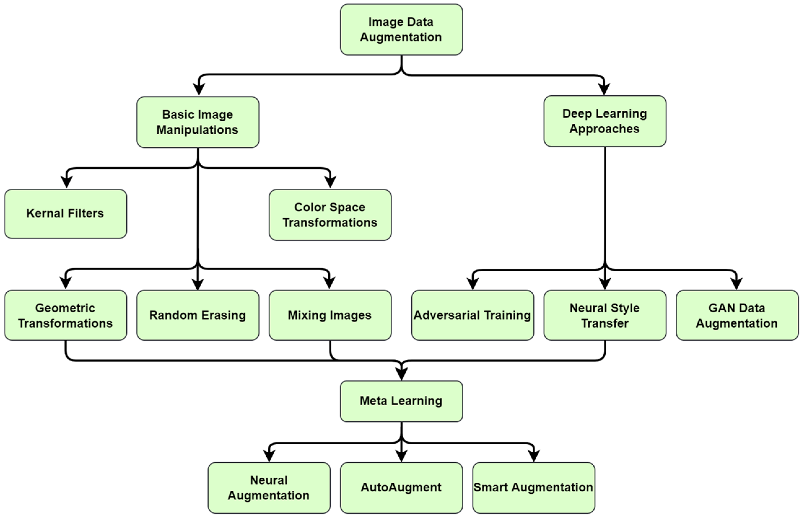
Figure 1. Summary of the most common data augmentation techniques [10].
Applsci 15 12321 g001
Figure 2. CutMix and SMOTE [26,27].
Applsci 15 12321 g002
Figure 3. (a). Representative samples of images used in the study [2]. (b). Schema of the proposed approach.
Applsci 15 12321 g003aApplsci 15 12321 g003b
Figure 4. Proposed pretrained model top layering.
Applsci 15 12321 g004
Figure 5. Model accuracy and loss curves on both training and validation (Set 1).
Applsci 15 12321 g005
Figure 6. Model accuracy and loss curves on both training and validation (Set 2).
Applsci 15 12321 g006
Figure 7. Model accuracy and loss curves on both training and validation (Set 3).
Applsci 15 12321 g007
Figure 8. Training accuracies pattern for all pretrained models on brightness augmentation.
Applsci 15 12321 g008
Figure 9. Validation accuracies pattern for all pretrained models on brightness augmentation.
Applsci 15 12321 g009
Figure 10. Training losses pattern for all pretrained models on brightness augmentation.
Applsci 15 12321 g010
Figure 11. Validation loss patterns for all pre-trained models on brightness augmentation.
Applsci 15 12321 g011
Figure 12. Evaluation metrics comparing custom-built model and pretrained models on baseline dataset.
Applsci 15 12321 g012
Figure 13. Model performance comparison for rotation augmentation.
Applsci 15 12321 g013
Figure 14. Model performance comparison for blur augmentation.
Applsci 15 12321 g014
Figure 15. Model performance comparison for brightness augmentation.
Applsci 15 12321 g015
Figure 16. Model performance comparison for noise augmentation.
Applsci 15 12321 g016
Figure 17. Model performance comparison for shear augmentation.
Applsci 15 12321 g017
Figure 18. Representative samples of the noise crack dataset [50].
Applsci 15 12321 g018
Table 1. Summary of model training behaviors across all augmentation techniques.
Pretrained ModelsShearBlurNoiseRotation
VGG-16Accuracies (MNF)Loss (NF)Accuracies (NF)Loss (NF)Accuracies (NF)Loss (NF)Accuracies (NF)Loss (NF)
Inception V3Accuracies (MJF)Loss (MJF)Accuracies (NF)Loss (NF)Accuracies (NF)Loss (NF)Accuracies (NF)Loss (NF)
ResNet50Accuracies (MNF)Loss (NF)Accuracies (MJF)Loss (NF)Accuracies (NF)Loss (NF)Accuracies (NF)Loss (NF)
EfficientNetB0Accuracies (NF)Loss (NF)Accuracies (MJF)Loss (MJF)Accuracies (MJF)Loss (MJF)Accuracies (MJF)Loss (MJF)
EfficientNetB7Accuracies (MNF)Loss (MNF)Accuracies (MNF)Loss (MNF)Accuracies (MNF)Loss (MNF)Accuracies (MNF)Loss (MNF)
ResNet152V2Accuracies (NF)Loss (NF)Accuracies (MJF)Loss (MJF)Accuracies (MNF)Loss (MNF)Accuracies (NF)Loss (NF)
DenseNet201Accuracies (NF)Loss (NF)Accuracies (NF)Loss (NF)Accuracies (MNF)Loss (MNF)Accuracies (NF)Loss (NF)
XceptionAccuracies (NF)Loss (NF)Accuracies (NF)Loss (NF)Accuracies (MNF)Loss (MNF)Accuracies (NF)Loss (NF)
InceptionResNetV2Accuracies (NF)Loss (NF)Accuracies (NF)Loss (NF)Accuracies (NF)Loss (NF)Accuracies (NF)Loss (NF)
NF = No significant fluctuations. MNF = Minor and relatively small fluctuations. MJF = Major fluctuations.
Table 2. Hyper-parameter optimization on the custom-built model.
Mini Batch SizeLearning RateAccuracyPrecisionRecallF1 ScoreTraining Time (s)Inference Time (s)
3210−150.121000.240.48181.742.16
10−250.000.000.000.00185.042.04
10−386.278.5599.687.83185.111.98
10−496.0493.6398.8096.15189.472.16
10−591.686.1699.1292.19186.081.98
6410−193.5695.5691.3693.42170.802.72
10−250.000.000.000.00172.662.57
10−394.8091.1298.2494.97173.642.57
10−495.6893.5298.096.0175.692.77
10−595.9294.0998.096.0170.272.53
128
10−150.000.000.000.00166.052.74
10−289.8883.3999.6090.78163.782.72
10−393.3689.4999.6893.75173.03.36
10−495.392.899.0495.5177.34.1
10−597.898.497.797.1170.183.58
No of conv. layer = 3.
Table 3. Custom-built model optimization for number of convolution layers.
No of Conv. LayersAccuracy
(%)
Precision
(%)
Recall
(%)
F1 Score
(%)
Training
Time (s)
Inference
Time (s)
168.9262.2995.9275.53102.242.61
290.5686.1196.7291.11150.482.49
397.898.497.797.1170.183.58
492.5287.9998.4892.94178.572.75
578.2869.7499.9282.14183.943.75
Learning rate = 10−5, mini-batch size = 128.
Table 4. Custom-built model optimization for optimizers.
Type of
Optimizers
Accuracy
(%)
Precision
(%)
Recall
(%)
F1 Score
(%)
Training
Time (s)
Inference
Time (s)
Adam 97.898.497.797.1170.183.58
RMSProp91.3291.9690.5691.25170.166.08
Adagrad 58.5458.6360.0859.34169.104.32
Learning rate = 10−5, mini-batch size = 128, no of conv. layer = 3.
Table 5. Custom-built model optimization for kernel sizes.
Kernel SizeAccuracy
(%)
Precision
(%)
Recall
(%)
F1 Score
(%)
Training
Time (s)
Inference
Time (s)
3 × 397.898.497.797.1170.183.58
5 × 592.287.6098.3292.65238.513.50
7 × 797.4895.5599.697.52329.474.21
Learning rate = 10−5, mini-batch size =128, no of conv. layers = 3, optimizer = Adam, loss function. = sparse categorical cross entropy.
Table 6. Evaluation metrics of the custom-built model on the baseline and augmented datasets.
Augmented Data
PrecisionRecallAccuracyF1 ScoreAUC
98.497.197.897.797.8
Unaugmented data
Blur92.0498.9695.2095.3795.20
Brightness89.1896.9692.6092.9192.60
Noise86.9492.0492.0892.6092.08
Rotation91.9199.0495.1695.3495.16
Shear98.9396.1697.5697.5397.56
Blur92.0498.9695.2095.3795.20
Table 7. Performance of models on real-world noise datasets.
Model Evaluation Metrics
ModelAccuracy Precision Recall F1 Score Training Time (s)Inference Time (s)
VGG-1697.29510097912
Inception V388.58398898412
ResNet5086.9957886718
EfficientNetB063.010026417114
ResNet152V294.6901009512020
EfficientNetB7
DenseNet20198.3971009812047
Xception97.29510097913
InceptionResNetV283.682868410322
Proposed Model97.610095.297.6272
Table 8. Summary of confusion matrices (Baseline).
CNN ModelsParameters
TPFPTNFN
VGG-16606190 2625 1
Inception V3612138617
ResNet506022322603
EfficientNetB0613120 2625 1
EfficientNetB7622 13 22623
ResNet152V261872623
DenseNet201614119616
Xception61693622
InceptionResNetV26071812613
Proposed ResNet6151018607
1 Signifies the highest number of True positives (TP) and True negatives (TN). 2 Signifies the least number of False positives (FP) and False negatives (FN).
Table 9. Summary of confusion matrices (Rotation).
CNN ModelsParameters
TPFPTNFN
VGG-161222 128 221248
Inception V3116585151235
ResNet501085165311219
EfficientNetB01173770 21250 1
EfficientNetB711826811249
ResNet152V211539731247
DenseNet201121238171233
Xception12203031247
InceptionResNetV2121040201230
Proposed ResNet1141109121238
1 Signifies the highest number of True positives (TP) and True negatives (TN). 2 Signifies the least number of False positives (FP) and False negatives (FN).
Table 10. Summary of confusion matrices (Blur).
CNN ModelsParameters
TPFPTNFN
VGG-161219 131 241246
Inception V3114810271243
ResNet50116783431207
EfficientNetB011876711249
EfficientNetB71193570 21250 1
ResNet152V2114710321248
DenseNet201121634111239
Xception12113961244
InceptionResNetV211628881242
Proposed ResNet1098152161234
1 Signifies the highest number of True positives (TP) and True negatives (TN). 2 Signifies the least number of False positives (FP) and False negatives (FN).
Table 11. Summary of confusion matrices (Brightness).
CNN ModelsParameters
TPFPTNFN
VGG-161222 128 221248
Inception V3113911181242
ResNet501146104351215
EfficientNetB0113911101250
EfficientNetB71222 128 20 21250 1
ResNet152V211648661244
DenseNet201122228141236
Xception12113961244
InceptionResNetV211549661244
Proposed ResNet1092158231227
1 Signifies the highest number of True positives (TP) and True negatives (TN). 2 Signifies the least number of False positives (FP) and False negatives (FN).
Table 12. Summary of confusion matrices (Noise).
CNN ModelsParameters
TPFPTNFN
VGG-1612084211249
Inception V3113911171243
ResNet50115298411209
EfficientNetB01183670 11250 1
EfficientNetB71217 133 20 21250 1
ResNet152V211579321248
DenseNet20112044611249
Xception12104011249
InceptionResNetV211807071243
Proposed ResNet1064186121238
1 Signifies the highest number of True positives (TP) and True negatives (TN). 2 Signifies the least number of False positives (FP) and False negatives (FN).
Table 13. Summary of confusion matrices (Shear).
CNN ModelsParameters
TPFPTNFN
VGG-1612232731247
Inception V3117575111239
ResNet501097153251225
EfficientNetB011975301250
EfficientNetB71217330 21250 1
ResNet152V211569441246
DenseNet201121535111239
Xception12232741246
InceptionResNetV2120545151235
Proposed ResNet1237 113 2481202
1 Signifies the highest number of True positives (TP) and True negatives (TN). 2 Signifies the least number of False positives (FP) and False negatives (FN).
Table 14. Comparison of model computational efficiency and complexity.
Model Parameters
ModelParameter (in Millions)Size
(Mb)
DepthFLOPsTraining Time (s)
VGG-16138.45281616 G839
Inception V323.9921896 G331
ResNet5025.6981074 G482
EfficientNetB05.3291320.39 G323
ResNet152V260.423230711 G1003
EfficientNetB766.72564380.37 G1615
DenseNet20120.2804024 G820
Xception22.9888111 G694
InceptionResNetV255.921544915.1 G666
Proposed Model7.4828.540.296 G170
Disclaimer/Publisher’s Note: The statements, opinions and data contained in all publications are solely those of the individual author(s) and contributor(s) and not of MDPI and/or the editor(s). MDPI and/or the editor(s) disclaim responsibility for any injury to people or property resulting from any ideas, methods, instructions or products referred to in the content.