Hybrid Physics-Informed Neural Network Correction of the Lotka–Volterra Model Under Noisy Conditions: Sensitivity Analysis of the λ Parameter

Abstract

In recent years, hybrid systems combining data-driven and physics-based approaches have gained increasing attention for solving complex real-world problems where deterministic modeling alone is insufficient. Within this framework, Physics-Informed Neural Networks and related hybrid models have been successfully applied across physics, engineering, and biological systems to improve predictive accuracy under uncertainty. However, their stability and sensitivity to noise and model misspecification remain open questions. This study investigates a hybrid Lotka–Volterra population dynamics model augmented with a neural correction term, aiming to analyze how the strength of the neural contribution, controlled by the coupling parameter $\lambda$ ($0\le \lambda \le 1$), affects model performance under noisy and distorted conditions. Here, $\lambda =0$ corresponds to the purely physical Lotka–Volterra system, whereas $\lambda =1$ represents the fully neural-corrected model. Three experimental setups were implemented: (1) evaluation on noisy data, (2) analysis of the $\lambda$ sensitivity and its stabilizing effect, and (3) compensation of parameter distortion through neural adaptation. The results indicate that, in the absence of parameter-induced distortions, relying solely on noisy data, moderate neural correction provides the most accurate and stable model behavior, whereas excessive neural influence may distort the original system dynamics. Conversely, when the underlying Lotka–Volterra model incorporates biased parameters, neural correction with a higher $\lambda$ effectively compensates for structural inaccuracies, enhancing predictive robustness.

1. Introduction

The modeling of ecological systems plays a crucial role in the study of population dynamics. One of the most well-known and widely cited formalisms for the mathematical description of prey–predator interactions is the Lotka–Volterra (LV) model, a system of differential equations that has played a defining role in ecological dynamics research since the 1920s [1]. However, it also exhibits several limitations: for instance, it assumes a homogeneous environment, constant parameters, and a simple linear form of interactions [2]. Empirical data are often noisy and subject to nonlinear effects, which reduce the purely deterministic predictive capability of the LV model.

In recent decades, applications of artificial intelligence (AI) have undergone remarkable advancement, and their use has become widespread across various fields of science and technology. AI-based methods, particularly the hybridization of intelligent algorithms, have enabled the efficient and effective solution of complex real-world problems that are difficult or even impossible to address using traditional deterministic approaches [3,4,5,6].

Significant progress has been made in the field of Physics-Informed Neural Networks (PINN) and hybrid modeling approaches [7]. These methods combine classical differential equation–based models with the flexibility of neural networks (NN). The objective is for the neural component to compensate for structural deficiencies in the model while the differential equation ensures physical or ecological coherence. Several studies in the literature have incorporated neural networks into parameter estimation for ecological models [8]. However, an important question arises: under what conditions does the neural network component provide genuine advantages compared to the classical model?

The hybrid residual correction with $\lambda$-weighting represents a less-explored approach. This weighting parameter regulates the relative contribution of the neural correction to the classical LV dynamics. The aim of the present study is to investigate the hybrid LV–NN model. By adjusting the $\lambda$ parameter, we determine the extent to which the neural network contributes to the prediction compared to the purely mathematical model. Consequently, this study seeks to address the following research questions:

• To what extent can the neural network improve the fit of the classical LV model when applied to noisy data?
• How does the variation in the $\lambda$ parameter influence the model’s performance, and under what circumstances does the neural correction provide genuine added value?
• In which cases is $\lambda =0$ optimal—no neural contribution—and when can higher $\lambda$ values be observed to enhance predictive accuracy?

At the beginning of the paper, international studies addressing similar problems are presented. This is followed by the methodology section, which aims to provide an overview of the mathematical formalism and theoretical background of the Lotka–Volterra model, as well as to introduce the hybrid modeling approach combined with neural networks and the specific solutions applied in this research. This includes the generation of simulated and noisy datasets, the architecture of the employed neural networks, and the procedure used to determine the optimal $\lambda$ value based on the loss function. The fourth chapter discusses the results, presenting the model’s fitting performance under different $\lambda$ values, the loss function curves, and the visualization of prey–predator dynamics. The fifth chapter focuses on the interpretation of the results, the answers to the research questions, and the summary of the main conclusions, while also outlining the existing limitations and proposing directions for future development.

2. Related Work

Several studies have addressed the extension of PINNs to handle noisy measurements, typically Gaussian noise as well as model inaccuracies [9,10,11]. Pilar and Wahlström demonstrated that the standard PINN approach may become unreliable in the presence of non-Gaussian noise and proposed the joint training of energy-based models (EBMs) to learn the noise distribution. This allows the PINN’s data loss to be aligned with the true measurement likelihood, implying that the nature of noise fundamentally determines the conditions under which a PINN-based solution can be applied reliably [12].

Within the field of population modeling and population balance (PBL-type) problems, the application of physics-informed approaches has also gained attention. In a recent study, Ali (2025) employed PINN-based, data-driven networks to compensate for deficiencies in mechanistic models and found that neural components adhering to the underlying physical structure while fitting observational data can significantly enhance estimation and model fitting performance—particularly in cases where measurement noise or certain parameters cannot be directly modeled [13].

Rapid progress has also been observed in the application of PINNs within ecological and vector-transmission modeling contexts. In their study, Lalic et al. specifically examined how PINNs can assist in the inverse estimation of parameters in mechanistic (Ordinary Differential Equation—ODE-based) models. They compared PINN-based solutions with classical mechanistic models and found that the PINN approach often delivers superior performance, particularly in cases where the accuracy of the mechanistic model is limited [14].

The use of PINN frameworks is also expanding in more specific ODE optimization problems. The study by Cuong et al. investigates the adaptation of PINNs to improve the estimation performance of ODE-based population models [15].

In addition to their own results, Yang and Li’s study provides a detailed introduction to parameter estimation methods for nonlinear dynamic systems [16]. The field has been extensively studied using both classical and modern approaches. Traditional methods such as Extended and Particle Kalman Filters, Bayesian inference, and adaptive filtering have shown strong theoretical foundations but often struggle with noisy or limited data [17,18,19].

More recent research has shifted toward neural approaches that combine the expressiveness of deep learning with the interpretability of physical modeling. The introduction of Neural Ordinary Differential Equations (Neural ODEs) by Chen et al. [20] established a continuous-time formulation for learning dynamical systems directly from data. Subsequent extensions, such as the Bayesian Neural ODEs of Dandekar et al. [21], further improved uncertainty quantification and robustness in parameter estimation tasks.

These developments highlight the growing interest in hybrid physical–neural models, where the integration of physical priors and neural corrections enables accurate system identification under high noise and data scarcity—a direction that also motivates the present study.

The reviewed literature consistently reflects a central insight that also underpins the motivation of the present study: the combination of physical models and neural networks can be advantageous, yet the key to effective integration lies in the nature of the noise, the specificity of the models, and the method of integration. Accordingly, the current study investigates the sensitivity of corrective weights through the application of PINN-like principles. The approaches and methods employed are aligned with the common recommendations highlighted in the aforementioned studies.

3. Materials and Methods

Population dynamics models constitute one of the oldest sets of tools for studying biological systems. Simpler approaches, such as exponential or logistic growth models, provide important insights into the fundamental growth tendencies of populations; however, they are incapable of capturing interactions between different species, as these cases involve single-population models studied within closed systems [22,23]. Natural phenomena, such as predator–prey cycles, exhibit far more complex dynamics, for which the classical Lotka–Volterra equations provide a foundational modeling framework. The LV system investigated in this study describes the temporal changes in two interacting populations using differential equations [1]:

$$\begin{gathered} {\displaystyle \frac{dx}{dt}}=x\left(\alpha -\beta y\right), \\ {\displaystyle \frac{dy}{dt}}=y(\delta x-\gamma ), \end{gathered}$$

(1)

where $x(t)$ represents the prey population, while $y(t)$ denotes the predator population as functions of time. The parameter $\alpha$ corresponds to the prey’s reproductive rate, $\beta$ reflects the predation rate, $\delta$ represents the predator growth resulting from prey–predator encounters, and $\gamma$ denotes the natural mortality rate of the predators. Solutions of the model typically exhibit periodic oscillations, intuitively reflecting the cyclical nature of prey and predator populations.

Although the Lotka–Volterra equations provide an important theoretical foundation, a primary limitation lies in their sensitivity to parameter inaccuracies. In real ecological systems, parameters are often difficult to measure, may vary over time, or are available only as approximate estimates. Consequently, predictions from the classical LV model can deviate from actual dynamics, particularly in the presence of noisy observations or errors in parameter estimation. To address this issue, we propose a hybrid approach that combines the classical Lotka–Volterra model with a neural network. Conceptually, the proposed hybrid modeling framework follows the principles of Physics-Informed Neural Networks, aiming to integrate prior physical knowledge into data-driven learning frameworks. Unlike the traditional PINN formulation—where governing differential equations are directly embedded into the loss function via physics-based residuals—the present model retains the explicit analytical form of the Lotka–Volterra equations and trains a neural network to learn the residual dynamics between the measured (noisy) data and the derivatives predicted by the model. This design choice renders the architecture more flexible and interpretable within the context of population dynamics, enabling the neural component to function as a data-driven corrective term that compensates for model inaccuracies, parameter distortions, and unmodeled environmental effects. The central idea is to augment the deterministic structure provided by the LV model with a learnable corrective term:

$${\displaystyle \frac{dz}{dt}}=f_{LV}\left(z,t;\theta \right)+\lambda f_{NN}\left(z,t\right),$$

(2)

where

• $z={[x,y]}^T$ is the state vector of the system, where $x(t)$ denotes the prey population and $y(t)$ denotes the predator population at time $t$;
• $f_{LV}\left(z,t;\theta \right)$ represents the deterministic component of the LV model, describing the classical prey–predator dynamics with the parameter vector $\theta =(\alpha ,\beta ,\delta ,\gamma )$;
• $f_{NN}(z,t)$ denotes the neural correction component, estimated by a multilayer perceptron (MLP), which aims to capture nonlinear or noisy behaviors not represented by the LV model;
• $\lambda \in \left[0,1\right]$ is a scaling factor that controls the extent to which the neural correction contributes to the overall dynamics;
• ${\displaystyle \frac{dz}{dt}}$ is the time derivative of the system, representing the population change predicted by the hybrid model.

The experiments and simulations were conducted in the MATLAB R2023a environment (MathWorks, Inc., Portola Valley, CA, USA) using the Deep Learning Toolbox and Signal Processing Toolbox modules. The classical trajectory was generated by numerically integrating the LV model with the use of the ode45 function [24]. To simulate the noise present in real-world data, additive Gaussian noise was introduced to the population trajectories:

$$Z_{obs}\left(t\right)=Z_{true}\left(t\right)+\epsilon \left(t\right),\epsilon ~N(0,{\sigma }^2)$$

(3)

where

• $\sigma$ denotes the standard deviation of the noise, $\sigma =0.5$;
• $Z_{true}\left(t\right)={\left[x\left(t\right),y(t)\right]}^T$ is the reference trajectory obtained by numerical integration of the classical LV equation;
• $Z_{obs}\left(t\right){=\left[x_{obs}\left(t\right),y_{obs}(t)\right]}^T$ represents the noise-corrupted dataset used for training the neural network.

Additive Gaussian noise is a well-established and commonly applied method for introducing stochastic perturbations into simulated population trajectories [25]. This ensures that the neural network learns not from “perfect” data but from realistic, noise-affected measurements. The objective of the neural network is to correct the deficiencies of the LV model. To achieve this, a numerical derivative was first computed from the noisy data:

$${\displaystyle \frac{d{Z}_{obs}}{dt}}\approx {\nabla }_{SG}{Z}_{obs}\left(t\right)$$

(4)

and then smoothed using a moving average to reduce the influence of noise. Following subsequent expert recommendations, the numerical smoothing procedure was extended by incorporating the Savitzky–Golay (SG) polynomial filtering method to obtain more robust derivative estimates (denoted by ${\nabla }_{SG}$). This approach preserves essential signal features while effectively suppressing high-frequency noise, improving the numerical stability of the hybrid model. The implementation followed MATLAB’s built-in sgolayfilt function description [26].

The difference between the model-derived and data-derived derivatives was defined as the residual error:

$$R\left(t\right)={\displaystyle \frac{d{Z}_{obs}}{dt}}-f_{LV}\left(Z_{obs}\left(t\right)\right)$$

(5)

where $f_{LV}$ denotes the right-hand side of the LV model.

Consequently, the objective function of the neural network is defined as:

$$\widehat{R}\left(t\right)\approx R\left(t\right).$$

(6)

A supervised regression neural network was employed to approximate the residual error of the Lotka–Volterra model. The network input consist of the current values of the prey and predator populations, along with time, forming a three-dimensional input vector:

$$X\left(t\right)=\left[x\left(t\right),y\left(t\right),t\right].$$

(7)

The neural network was trained on discrete timepoints which was produced by ode45 solver, forming a supervised dataset $M=301$ samples corresponding to the numerical solution grid. Each training pair is defined as:

$$T=\left\{\left(X\left(t_i\right),R\left(t_i\right)\right),i=1,\dots ,M\right\}.$$

(8)

The network output represent the model correction of the derivatives of the two populations which the neural network estimates through by learning from the residual errors.

Between the input and output layers, one fully connected hidden layer was initially employed, followed by two hidden layers in later experiments. The architectural configuration (number of layers and neurons) was refined empirically based on experimental performance and stability analysis, as discussed later in the manuscript. During our initial experiments the first hidden layer consisted of 32 neurons, while the second contained 16 neurons. A Rectified Linear Unit (ReLU) activation function was applied between the layers [27]:

$$ReLU\left(z\right)=\mathit{max}\left(0,z\right).$$

(9)

The ReLU function was chosen because this nonlinear transformation is capable of expressing complex nonlinear patterns while remaining computationally efficient. Moreover, it avoids the saturation problem commonly observed in classical sigmoid or tanh activation functions [28]. The ReLU activation function was employed, consistent with the common practice in neural dynamical modeling due to its Lipschitz continuity and computational efficiency [16,29]. Based on both experimental results and literature findings, the two hidden layers provide sufficient complexity for learning nonlinear patterns, while remaining compact enough to avoid overfitting on the relatively small dataset [30]. In line with literature on neural ODEs and hybrid models, a fully connected network architecture was adopted [16].

The neural network was trained using the Adam optimizer for 200 epochs with an initial learning rate of 10⁻³, mini-batches of 32 samples, and $L_2$ regularization (10⁻⁴). Inputs were normalized using z-score normalization at the feature layer to improve numerical stability and eliminate ordering bias, which settings follows MATLAB’s training procedure description [31]. The adaptive learning rate and fast convergence of the Adam algorithm enable stable and efficient training of the network, even on small or noisy datasets [32]. Following the reviewers’ suggestions, the training process was refined by shuffling data samples at every epoch to enhance convergence stability. To evaluate the robustness of the hybrid model, the entire training process was repeated across multiple random seeds, each corresponding to a distinct weight initialization of the network.

The resulting hybrid system thus represents a combination of the classical LV model and the neural correction component, formulated in MATLAB as follows:

$$f_{hybrid}(t,z)=f_{LV}(t,z)+\lambda \widehat{R}(t,z),$$

(10)

where the weighting parameter $\lambda \in [0,1]$ controls the contribution of the neural correction as follows:

• $\lambda =0$ means purely LV model;
• $\lambda =1$ means full neural correction.

The model performance was evaluated based on its fit to the noisy observations. The Root Mean Square Error (RMSE) was computed separately for each component [6,33]:

$$\begin{gathered} {\mathrm{R}\mathrm{M}\mathrm{S}\mathrm{E}}_x=\sqrt{{\displaystyle \frac{1}{N}}\sum _{i=1}^N{(x_{hybrid}\left(t_i\right)-x_{obs}\left(t_i\right))}^2,} \\ {\mathrm{R}\mathrm{M}\mathrm{S}\mathrm{E}}_y=\sqrt{{\displaystyle \frac{1}{N}}\sum _{i=1}^N{(y_{hybrid}\left(t_i\right)-y_{obs}\left(t_i\right))}^2.} \end{gathered}$$

(11)

In this study, the optimal value of $\lambda$ was determined based on the minimization of the RMSE.

4. Results

The model performance was examined under three different configurations, designed to test the learning capability of the neural correction and the stability of the hybrid system. In all three cases, the Lotka–Volterra model served as the basis for the “true” dynamics, while the neural network learned corrective adjustments from the residual errors. The classical LV system operated with constant parameters ($\alpha ,\beta ,\gamma ,\delta$), which remained unchanged throughout the experiments, implying that the model was structurally time-invariant. The neural component did not estimate these parameters directly; instead, it learned to dynamically correct the modeling errors arising from them. The main objective was to observe when and to what extent the neural component improves the predictive performance of the classical model.

Figure 1 presents the simulation of the classical Lotka–Volterra model with fixed constant parameters ($\alpha =1.0,\beta =0.1,\delta =0.075,\gamma =1.5$). The initial population values were set to $x_0=10$ and $y_0=5,$ and the simulation was performed over the time interval $t\in \left[0,30\right].$ The system of differential equations (Equation (1) was numerically solved using MATLAB’s ode45 function. The resulting curves illustrate the temporal dynamics of the prey (x—shown in blue) and predator (y—shown in red) populations. The obtained results exhibit the characteristic periodic oscillations of the system: the increase in the prey population is followed by a rise in the number of predators, which in turn leads to a decline in the prey population, after which the predator count decreases, and the cycle repeats.

4.1. Instability in the Hybrid Lotka–Volterra–Neural Model and the Phenomenon of Drift

As an extension of the classical Lotka–Volterra model, a hybrid system was developed in which an artificial neural network was employed to correct the dynamics described by the differential equations. The aim was for the network, trained on noisy observations, to learn to reduce the model’s errors, thereby bringing the simulated trajectory closer to the “real” data.

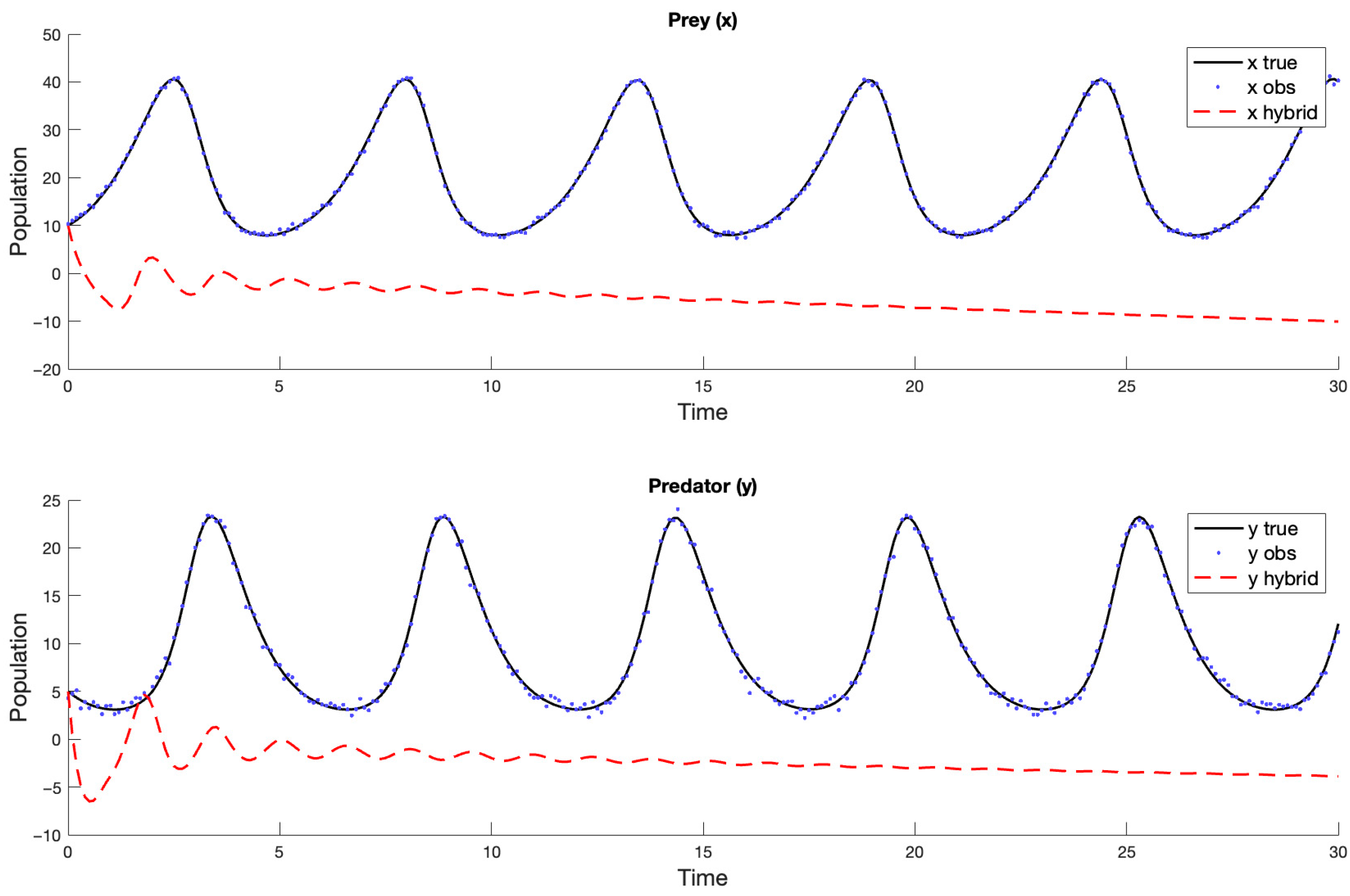
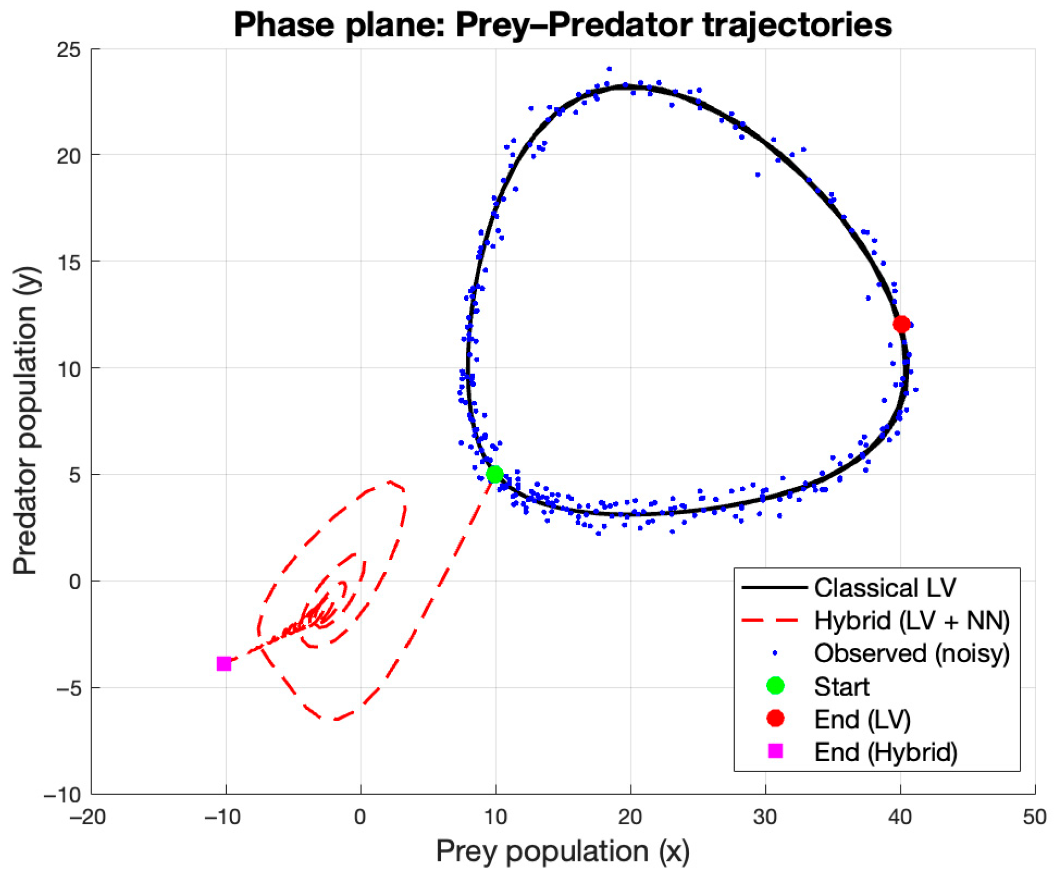
In the first iteration of the model, a simple neural network architecture was employed, consisting of a single hidden layer with 16 neurons and a ReLU activation function. The input data were fed directly into the network without prior normalization. The output layer represented two dimensions, corresponding to the correction values for the derivatives of the prey and predator populations. Training was performed using the Adam optimizer over 200 epochs with a batch size of 64. The experiments shown in Figure 2 and Figure 3 clearly demonstrate the inaccuracy of the neural network.

Upon examining the simulation results, it was observed that the trajectory computed from the hybrid model (red dashed line) gradually drifted away from the region defined by the classical LV model (black line) and the noisy observations (blue dots). Consequently, the system became unstable, the population values either decreased or increased unrealistically over time, and the simulation dynamics failed to remain within a biologically simulated plausible range.

During the analysis of the experimental settings, several sources of instability in the system were identified. The numerical derivatives computed directly from the noisy observations significantly distorted the target function. As highlighted in the literature, conventional finite-difference-based numerical differentiation is highly sensitive to noise, and even minor measurement errors can cause substantial distortion in the estimated derivatives [34]. Consequently, the neural network learned the noise rather than the model discrepancy, resulting in unstable training. As a result, when $\lambda =1$, the correction estimated by the neural network was fully added to the Lotka–Volterra dynamics. This complete weighting led to uncontrolled error amplification. Furthermore, since the input data were fed into the network without preprocessing, the model suffered from convergence instability. Given that the prey and predator population values differ in magnitude, the absence of normalization likely caused biased parameter learning within the network. Similar observations have been reported in PINN research, where improper scaling of input variables complicates optimization and introduces excessive error when fitting physical laws [35].

The first hybrid model experiment was therefore unstable, and the neural network failed to learn a meaningful correction for the model. Instead, the network captured fluctuations originating from the noise, which progressively amplified the deviations during numerical integration. This outcome clearly illustrates that incorporating a neural network into dynamical modeling leads to improvement only when the training data are properly preprocessed and when the neural correction exerts a constrained influence on the underlying model.

4.2. Stability Analysis of the Hybrid Lotka–Volterra–Neural Model Under Varying $\lambda$ Values

The objective of the second experiment was to stabilize the neural correction model that had produced unstable results in the first trial and to examine in detail how the magnitude of the neural correction influences the behavior of the hybrid system. The modifications primarily focused on improving the model’s numerical stability and mitigating the distortions in learning caused by noise. The neural network architecture was also revised to enhance the stability and accuracy of the training process. The single-layer network with 16 neurons used in the initial experiment exhibited underfitting, as it struggled to extract the true dynamical patterns from the noisy derivatives. Therefore, in the second experiment, a deeper architecture consisting of two hidden layers (with 32 and 16 neurons, respectively) and ReLU activations was employed. The numerically derived values obtained from noisy observations were smoothed using a moving average filter (with a five-point window), since gradient-based differentiation is highly sensitive to noise—a factor that significantly distorted the learning process in the previous experiment. By applying the smoothing procedure, the noise component originating from the numerical derivatives was successfully reduced, allowing the neural network to learn to correct the actual deviations of the Lotka–Volterra model rather than random noise. The normalization of the input variables further improved model stability by preventing input variables of different magnitudes from distorting the weight updates during training. To reduce the risk of overfitting, $L_2$ regularization (with a weight of 10⁻⁴) was incorporated into the training process. To examine the effect of the neural correction magnitude, simulations were conducted with multiple values of the $\lambda$ parameter ($\lambda =0.1,0.5,0.9$). As a result of these modifications, the hybrid system exhibited significantly improved stability. The neural network outputs closely followed the temporal variations in population dynamics, and the overall model predictions remained close to those of the classical LV model. 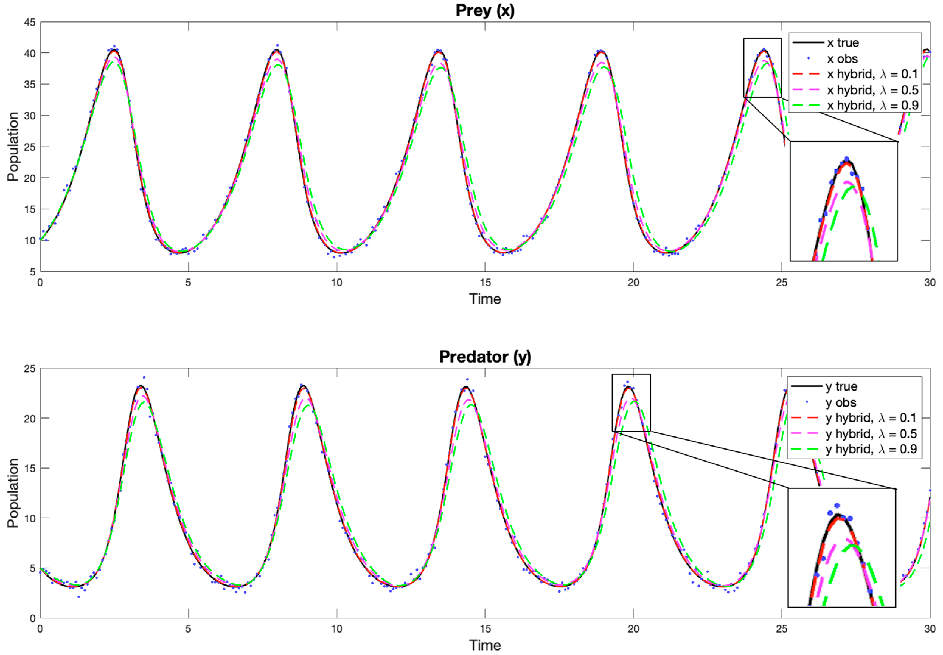Figure 4 and Figure 5 illustrates the population curves obtained for different $\lambda$ values, showing that while the neural corrections slightly deviate from the original LV trajectories, they accurately preserve the main dynamical characteristics of the system.

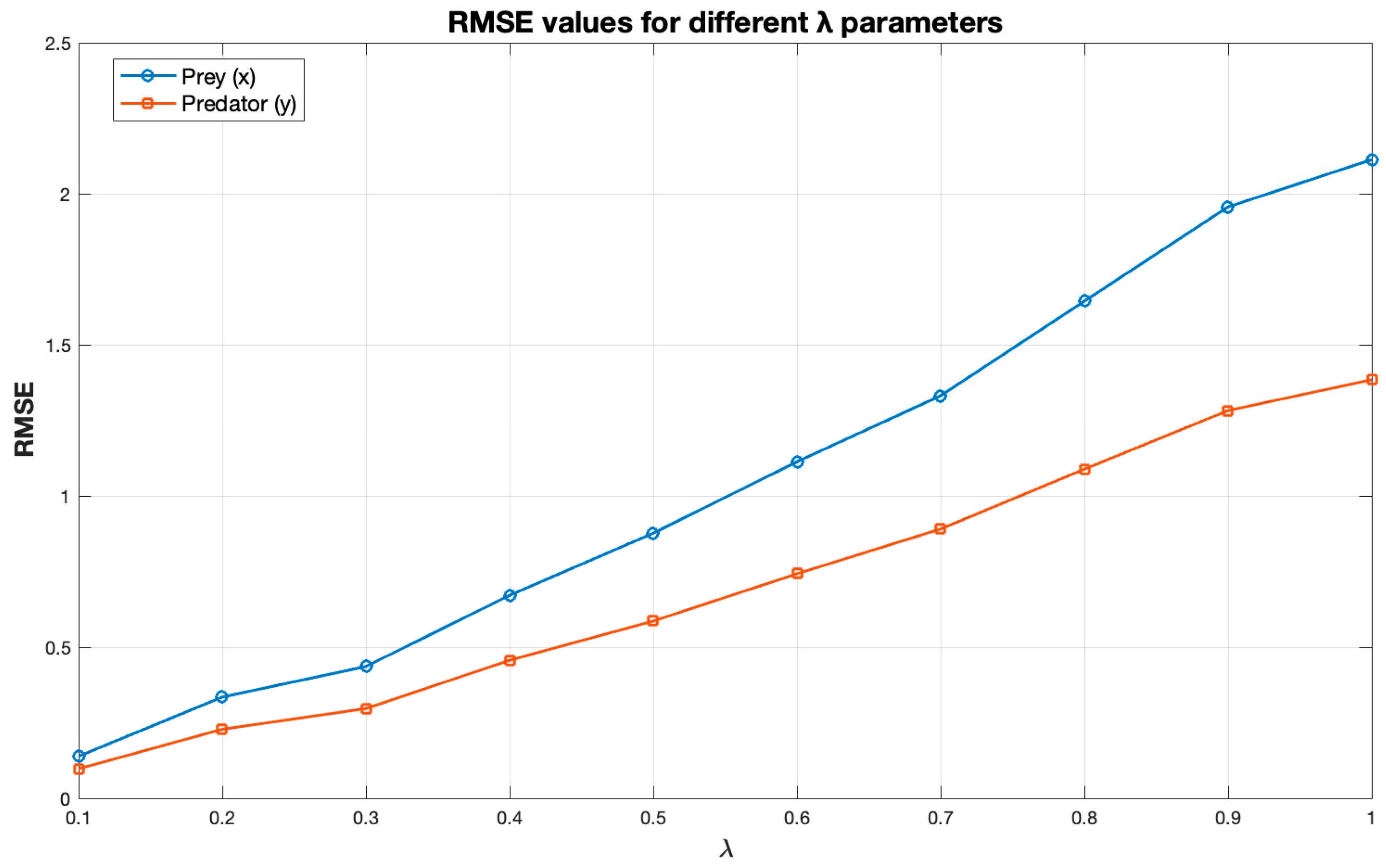
Figure 4 presents the fitting curves corresponding to different $\lambda$ values. Unlike in the first experiment (Figure 2), where the full neural correction (effectively $\lambda =1$) amplified the noise and produced drift, the present results demonstrate that a weaker correction (smaller $\lambda \approx 0.1–0.2$) yields a more accurate and stable fit to the noisy data. This is confirmed by the RMSE curve shown in Figure 6, plotted for different $\lambda$ values, evaluated in increments of $0.1$ within the range from $0.1$ to $1$. Nevertheless, higher $\lambda$ values (e.g.,$\lambda \approx 0.9$) still preserve the overall Lotka–Volterra oscillatory dynamics, indicating that the neural component remains consistent with the physical model structure even when its contribution is dominant, albeit slightly less precise.

Based on the results, it can be concluded that the smallest error was obtained with a moderate intensity of neural correction ($\lambda =0.1$), indicating that under these conditions the hybrid model achieved the highest accuracy. For larger $\lambda$ values, the corrections introduced by the neural network excessively influenced the system dynamics, leading to a deterioration in the model fit. This is an interesting observation, as it shows that although the prediction obtained with the neural network performed better than in the previous experiment, it still did not reach the accuracy of the classical LV output. Consequently, the true added value of the NN component within the system cannot yet be clearly observed.

4.3. Evaluating the Effectiveness of the Neural Correction Under Parameter-Biased Conditions

The aim of the third experiment was to investigate the extent to which the neural network could compensate for parameter distortions in the classical LV model ($\alpha =0.9,\beta =0.12,\delta =0.06,\gamma =1.7$), and under what conditions the neural correction can be considered effective. For this purpose, the base model parameters were intentionally deviated from their original values, so the hybrid system was built upon a misparameterized LV model, which the neural network attempted to correct. Since real ecological systems often exhibit time-varying environmental conditions, the heterogeneity of the model is not merely a simulation experiment. Several recent studies have similarly examined the LV model using time-varying parameters on this basis [36,37]. These findings imply that the effectiveness of the neural correction can be particularly significant when the physically modeled components are only approximate and when the system parameters are not static but vary over time. In our experiment, the neural network inputs again consisted of the state variables and time, while its objective function was defined as the difference between the noisy measured derivative and the derivative computed by the biased model. The network was trained using the Adam optimizer for 200 epochs, retaining the regularization parameters proven effective in the previous experiment. 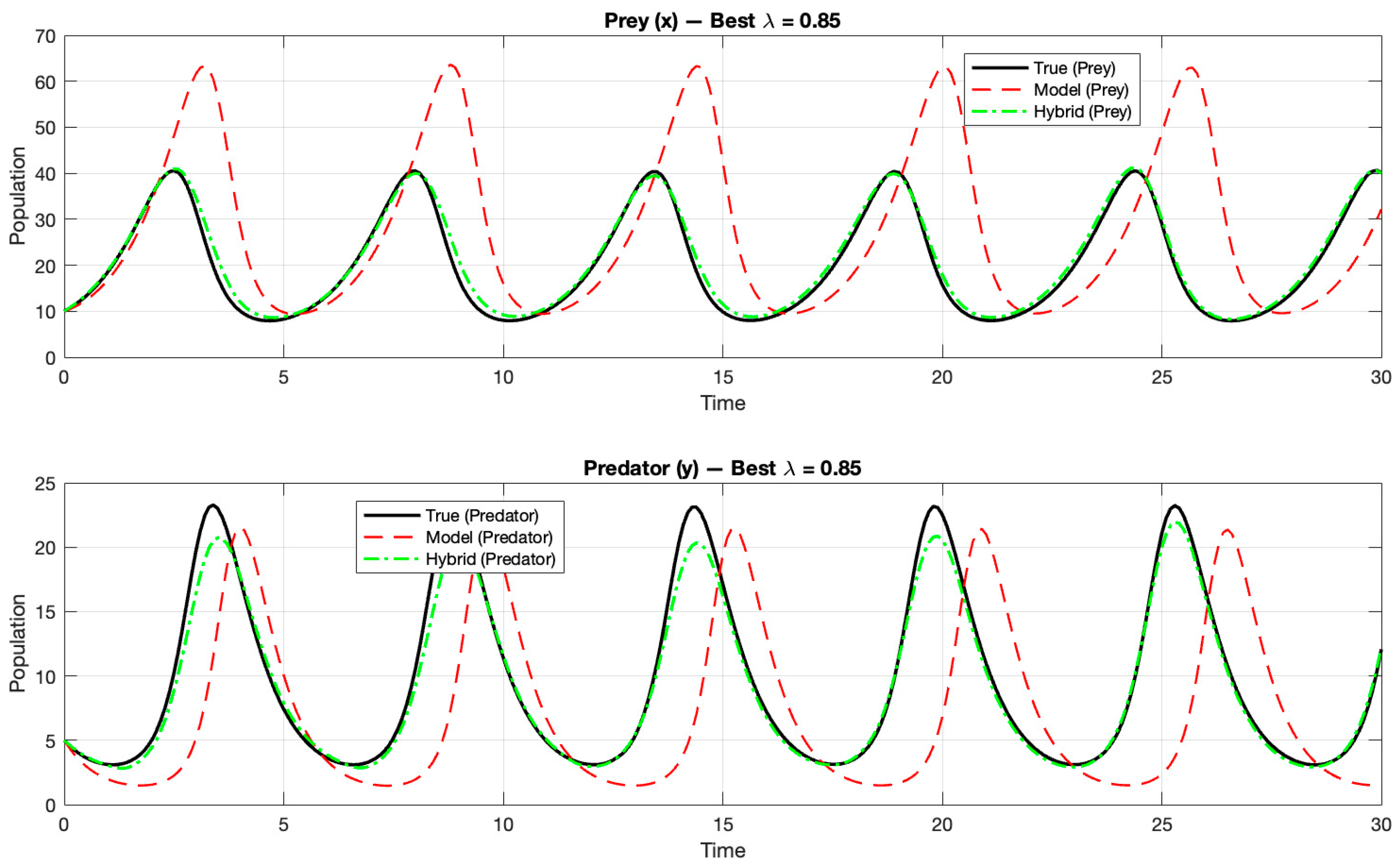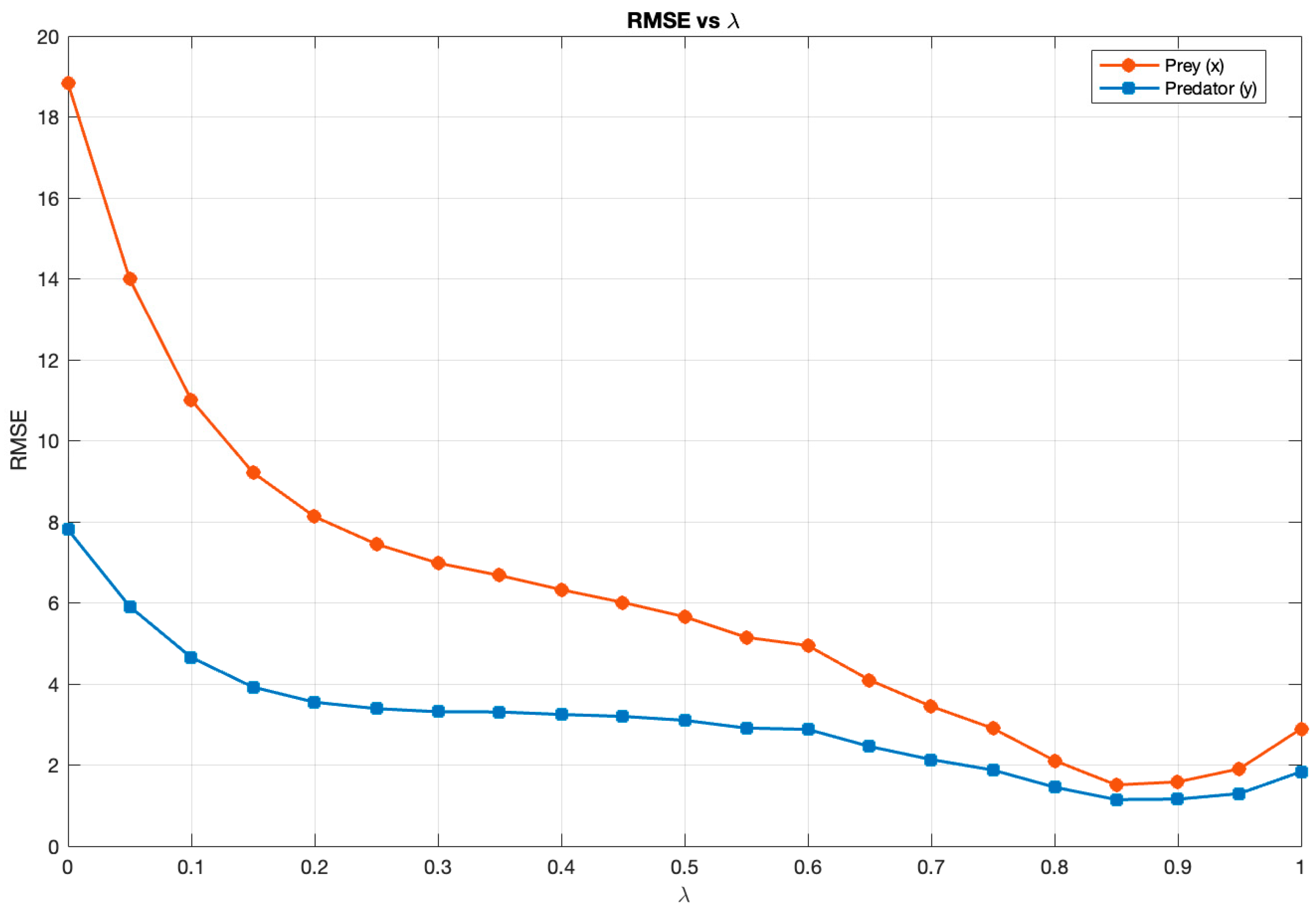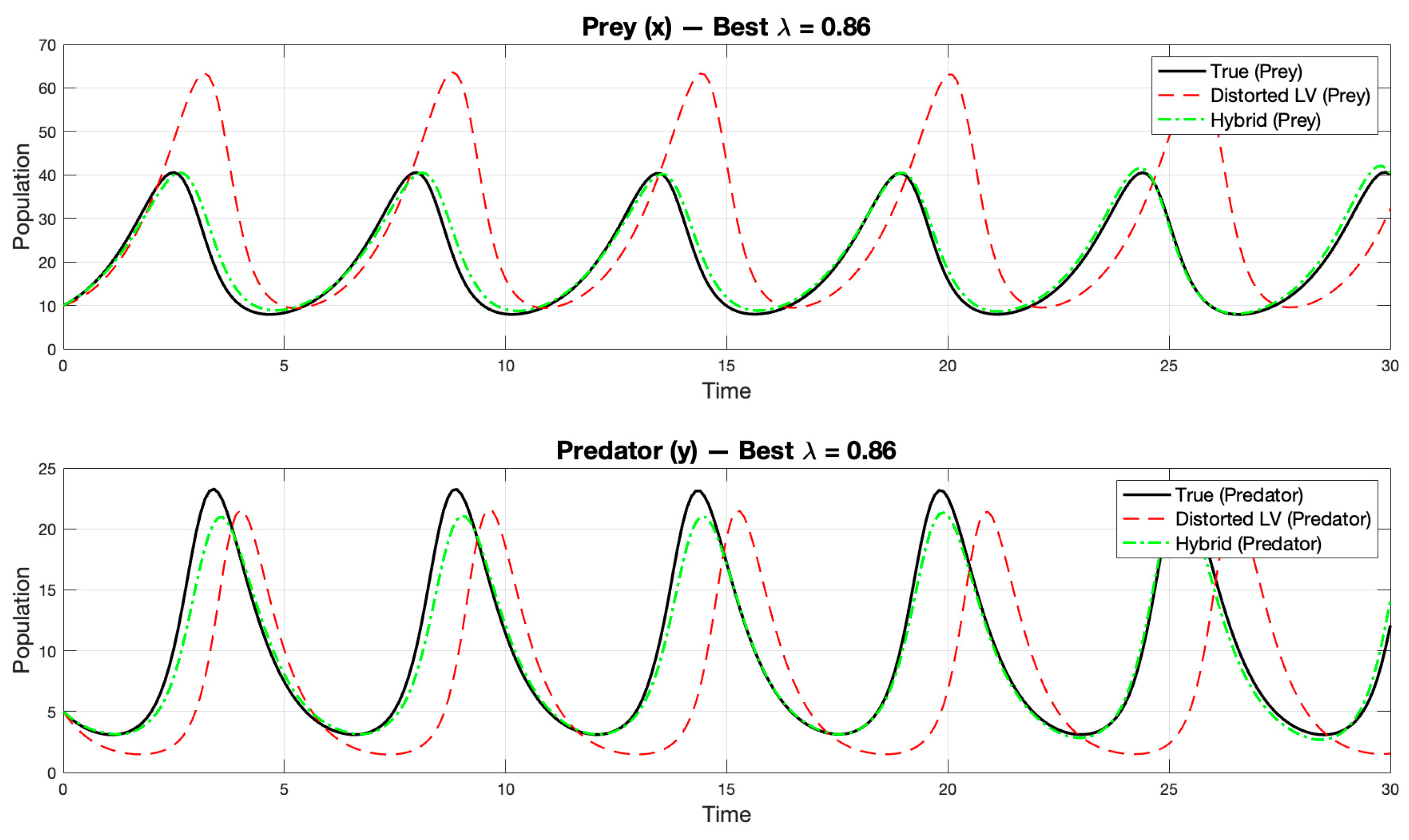During the experiment, the output of the hybrid model was evaluated for multiple $\lambda$ values (within the [0, 1] interval, with a step size of 0.05), based on the RMSE function. The results showed that the neural network was indeed able to improve the fit of the model operating with distorted parameters: the error metric decreased substantially with the application of the hybrid approach. The lowest RMSE was obtained at $\lambda =0.85$, indicating that the neural correction was most effective within this range. Figure 7 compares the temporal outputs of the classical, distorted, and hybrid models, while Figure 8 illustrates the variation in RMSE as a function of $\lambda$.

To quantitatively assess whether the neural correction in the hybrid model significantly improved the performance of the distorted LV system, we conducted a non-parametric statistical analysis comparing the two models’ residual errors over time.

The comparison was performed on paired samples taken at 301 equally spaced time points ($t_1=0,\dots {,t}_{301}=30$). Thus, for both the prey and predator variables, we obtained n = 301 paired observations of absolute error values for the two models.

Because the residuals did not meet normality assumptions, we applied the Wilcoxon signed-rank test to compare the distributions of model errors [38]. Although this test assumes independent paired samples, it was used here in a descriptive sense to provide an overall indication of median error differences. Given that the samples originate from temporally autocorrelated trajectories, the resulting p-values should be interpreted as qualitative indicators of systematic improvement rather than strict inferential statistics [39]. The hypotheses were formulated as follows:

H0. 

The median absolute errors of the hybrid and the distorted LV model are equal.

H1. 

The median absolute error of the hybrid model is lower than that of the distorted LV model.

The Wilcoxon signed-rank test results indicated consistently lower median absolute errors for the hybrid model across both prey and predator populations (prey: p = 3.68 × 10⁻⁴⁹; predator: p = 6.10 × 10⁻⁴⁸). Given the temporal dependence between consecutive samples, these results should be interpreted as descriptive indicators rather than formal hypothesis testing outcomes. Nevertheless, the consistent reduction in errors across the entire time domain supports the conclusion that the hybrid model provides systematically better performance than the distorted LV model. Therefore, the findings are in agreement with the alternative hypothesis. The effect sizes measured using Cohen’s $d_z$ were $d_{z,x}=0.86$ and $d_{z,y}=1.0$, which correspond to large effect sizes according to Cohen’s conventional thresholds [38]. Although the resulting p-values were extremely small this pattern is consistent with the highly systematic error reduction observed for the hybrid model across all time points, rather than indicating formal statistical significance. The large sample size and consistent direction of the error differences make the observed trend statistically stable and robust in a descriptive sense. 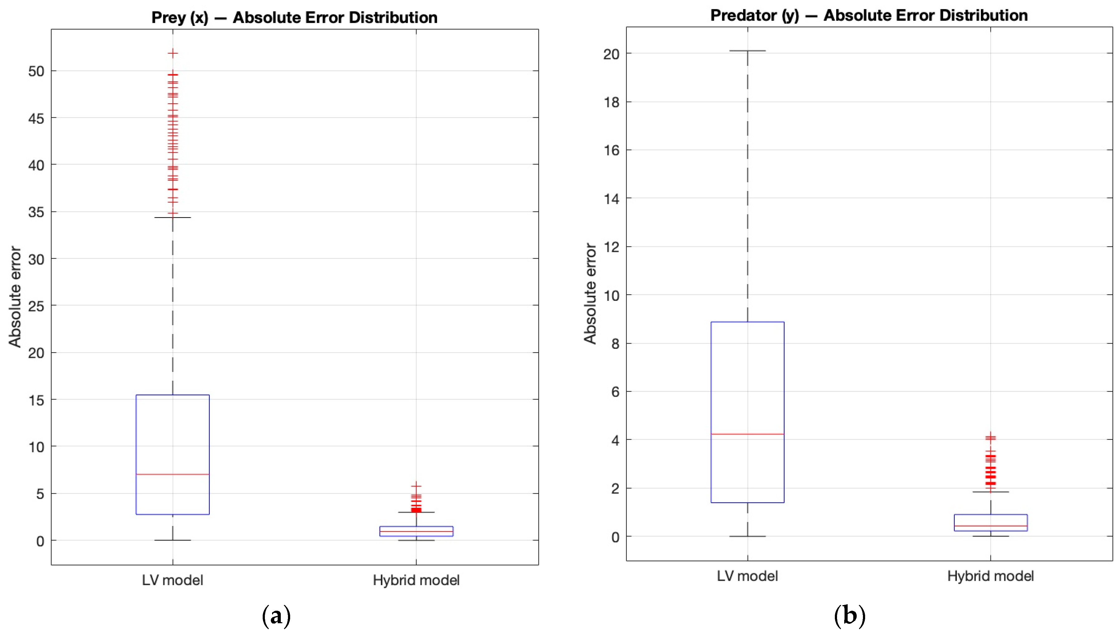Figure 9 presents the distribution of absolute errors for the prey and predator populations. The distorted LV model exhibits a much larger error variance and higher median compared to the hybrid model, whose distribution is compact and centered near zero.

Based on the results, it can be concluded that the stronger neural correction did not distort but rather compensated for the deviations caused by the incorrect parameters. This suggests that the neural network proves particularly effective when the uncertainties of the physical model stem from structural or parametric inaccuracies. In such cases, the neural correction does not alter the underlying dynamics but instead compensates for the missing or erroneous components, thereby enhancing the model’s predictive capability. This operating principle is consistent with the findings of PINN-style studies such as [40], where deficiencies in physical models were successfully mitigated through neural correction terms.

4.4. Extended Analysis with Filtered Data and Stochastic Robustness Testing

Following the reviewers’ valuable suggestions regarding the validation and robustness of the hybrid model, additional experiments were conducted to assess the stability and reliability of the previously presented results.

In particular, the reviewers emphasized the importance of employing more advanced differentiation techniques for noisy data and performing multi-seed validation to confirm the robustness of the hybrid framework.

In the original experiments, the numerical derivatives required for training the neural correction were estimated using a simple finite-difference approximation. However, this naïve approach was highly sensitive to measurement noise, which caused drift in the learned dynamics, as observed in Section 4.1.

To address this issue, the Savitzky–Golay polynomial smoothing and differentiation method was implemented to obtain more robust derivative estimates. This technique preserves key signal characteristics while effectively suppressing high-frequency noise [41]. The implementation followed MATLAB’s sgolayfilt function [26].

Figure 10 compares the naïve gradient-based derivatives and the Savitzky–Golay filtered derivatives for both prey and predator variables.

The results demonstrate that the simple gradient amplifies noise and produces irregular oscillations, whereas the Savitzky–Golay approach yields smooth and stable derivatives.

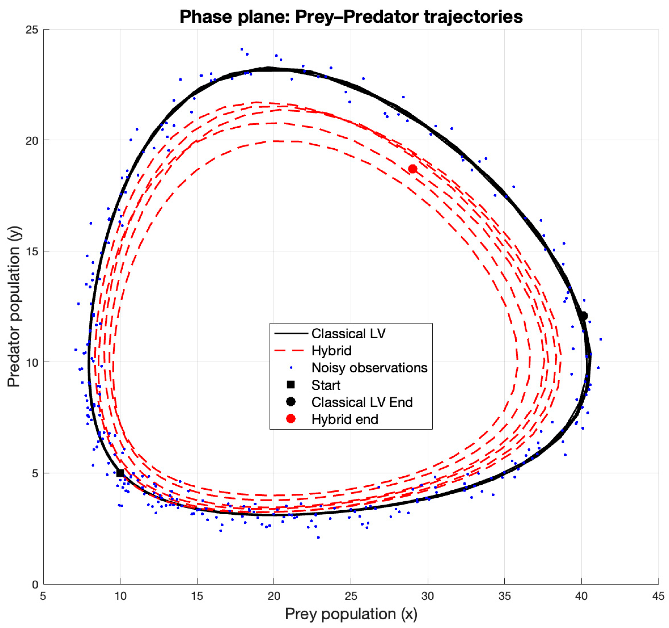
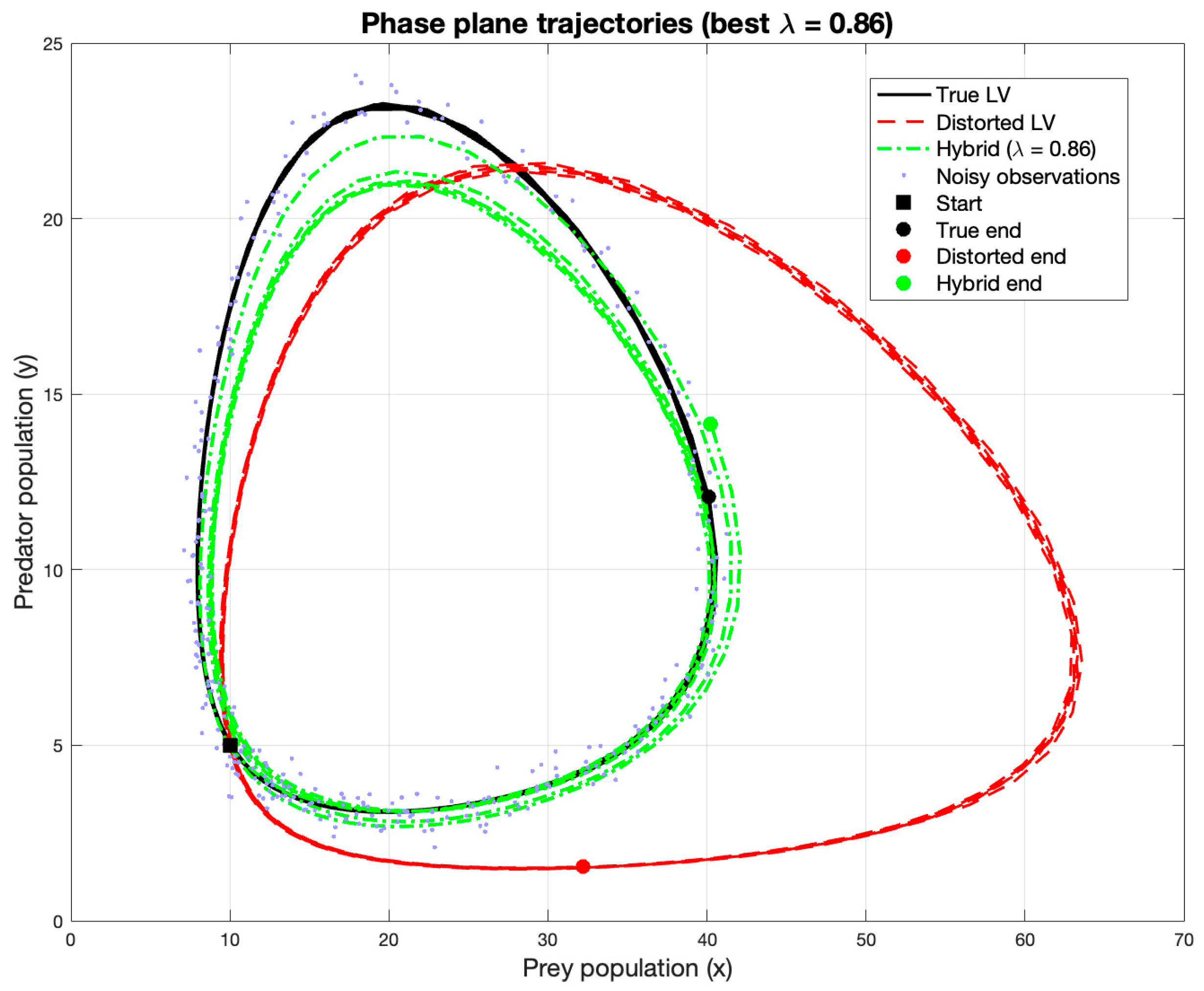
Consequently, the hybrid model trained with these improved derivatives exhibited significantly reduced drift and a closer alignment with the classical Lotka–Volterra trajectories in the phase plane as we can in Figure 11.

This test confirms that the previously observed drift originated primarily from noisy derivative estimates rather than from the hybrid modeling framework itself.

After applying Savitzky–Golay-based numerical differentiation in the second test, the RMSE–$\lambda$ curve remained consistent with the previous results demonstrated in Section 4.2. Although this filtering reduced local oscillations and yielded smoother derivative estimates, the optimal $\lambda$ still remained close to zero.

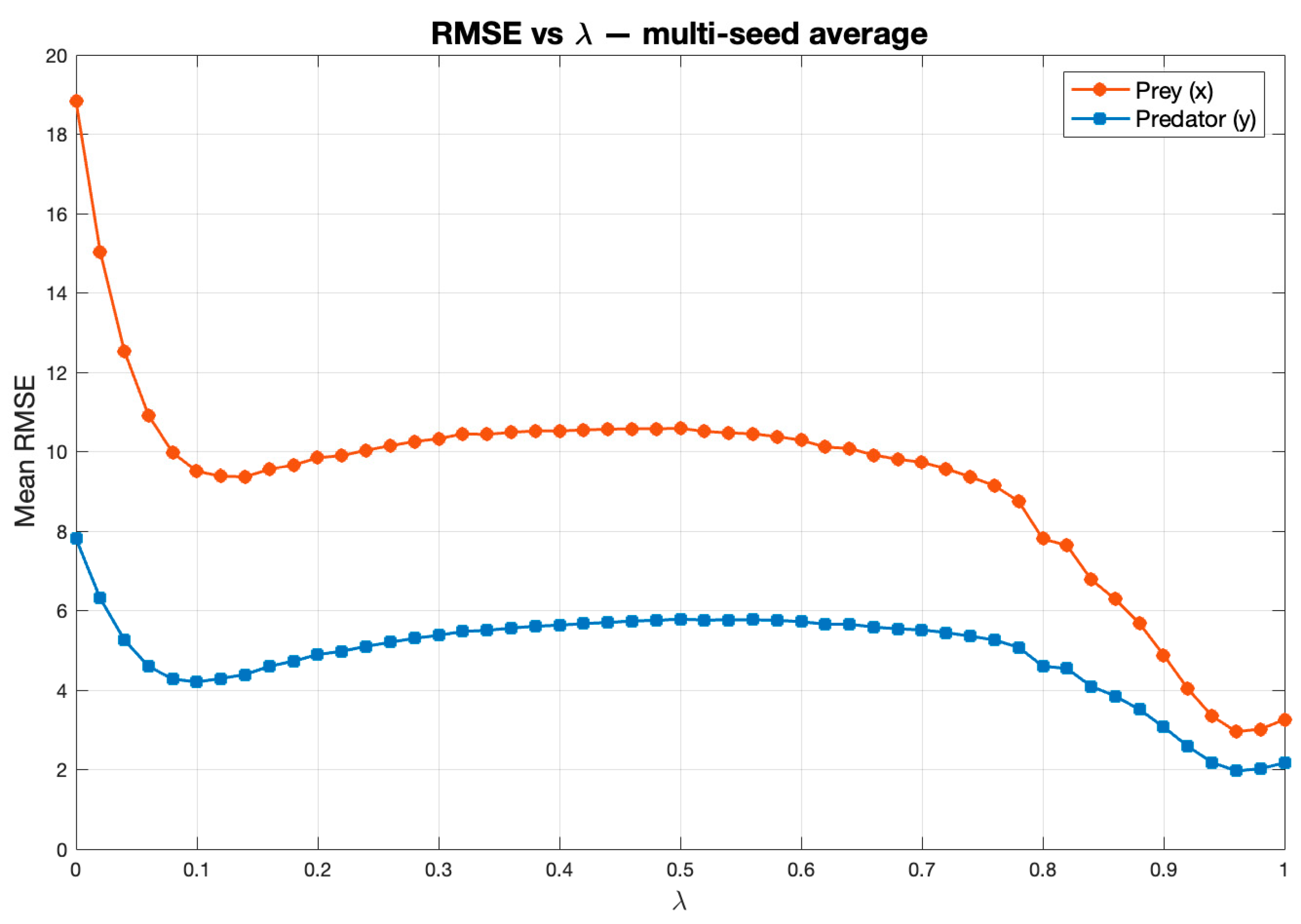
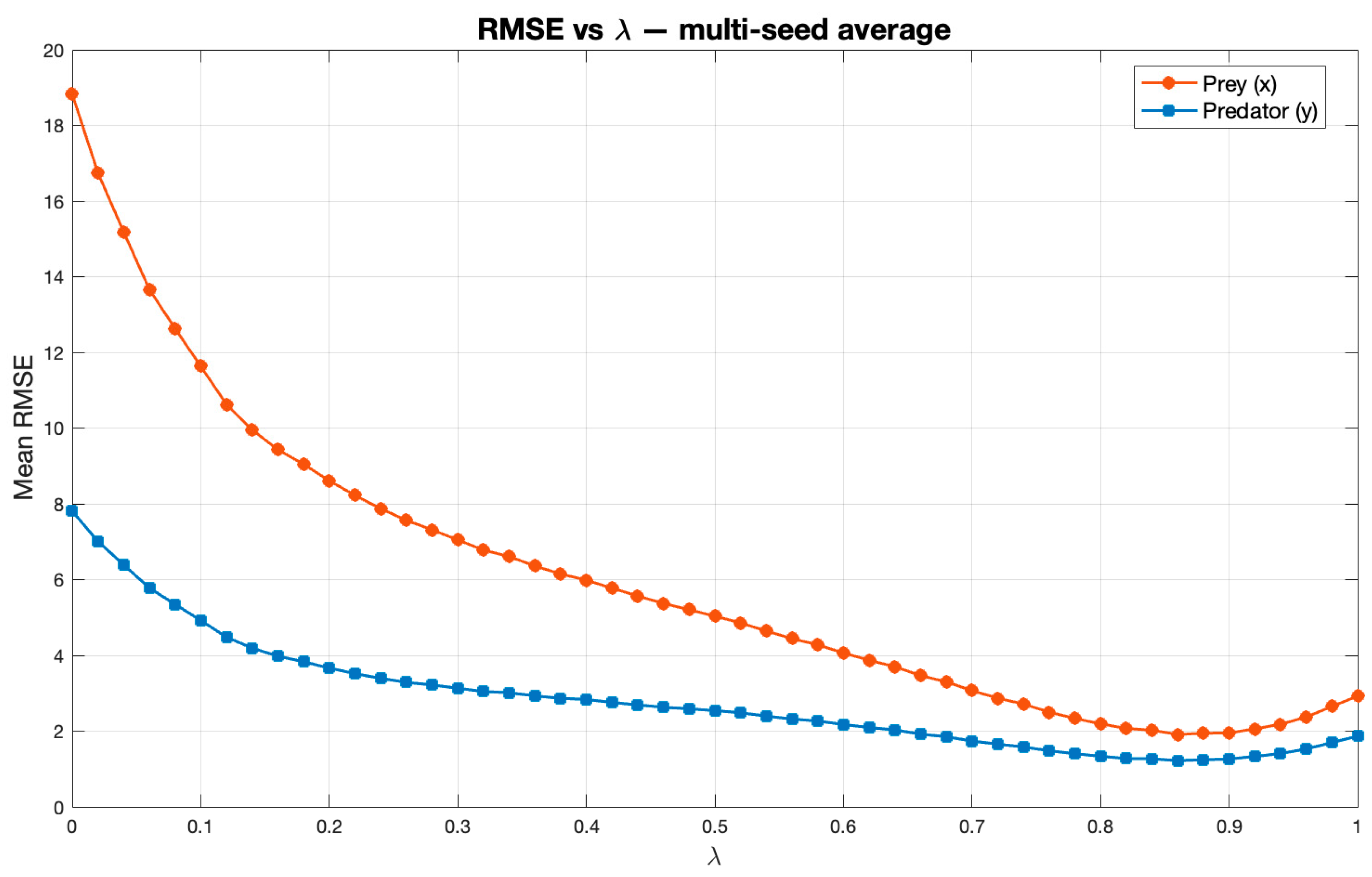
In the third experiment after filtering, the RMSE–$\lambda$ profile exhibited a noticeable shift: the minimum RMSE, previously around $\lambda \approx 0.85$, now appeared near $\lambda \approx 0.9–1.0$. To refine this observation, $\lambda$ values were tested with a smaller step ($\Delta \lambda =0.02$), producing a more detailed RMSE curve. To evaluate robustness, the neural network was retrained under three random seeds, each representing a distinct weight initialization. Additionally, mini-batch shuffling was enabled at every epoch to mitigate potential bias from data ordering. Across multiple neural architectures (1–3 hidden layers, 16–128 neurons), the results consistently demonstrated that the optimal $\lambda$ remained within 0.9–1.0.

These findings indicate that the hybrid model’s correction mechanism is robust to stochastic initialization and training randomness. Furthermore, the RMSE–$\lambda$ relationship revealed a steep initial improvement between $\lambda =0$ and $\lambda =0.1$, showing that even minimal neural correction rapidly compensates for parameter distortion. This was followed by a broad plateau region—indicating robustness to $\lambda$ variations—and a second improvement zone where RMSE reached its minimum near $\lambda \approx 0.94–0.98$ (prey RMSE ≈ 2.64; predator RMSE ≈ 1.87). 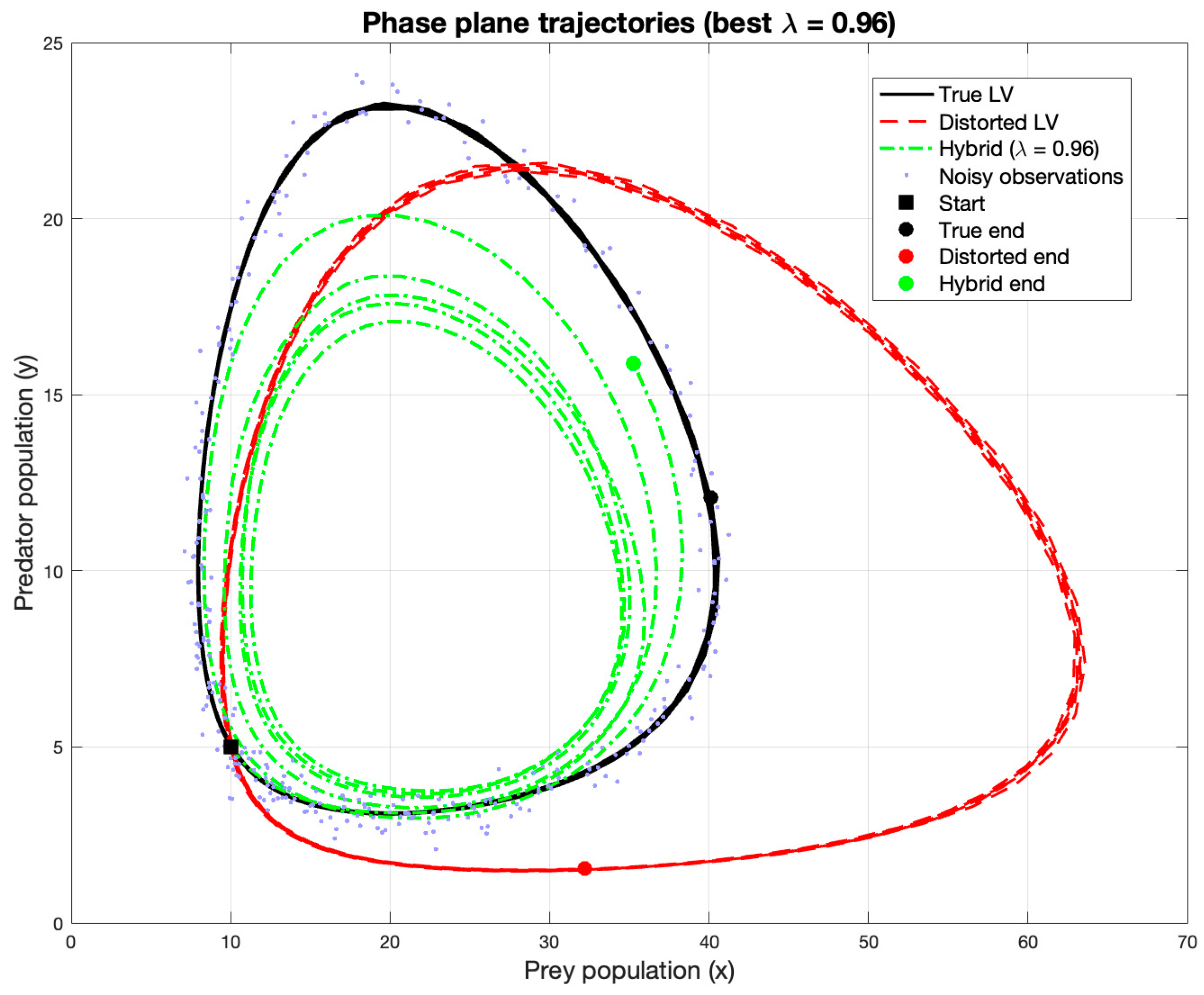Figure 12 illustrates the prey–predator phase-plane trajectories, where the black curve represents the true Lotka–Volterra dynamics, the red curve corresponds to the distorted-parameter model, and the green curve shows the hybrid model output obtained with the $\lambda$ value yielding the minimum RMSE. These results were produced after introducing the Savitzky–Golay smoothing method and training the neural network with multiple random seeds and shuffled mini-batches, in order to assess the robustness and consistency of the hybrid framework.

Across multiple seeds, the standard deviation of RMSE values decreased markedly for higher $\lambda$ values. In the near-optimal range ($\lambda \approx 0.9–1.0$), the deviations dropped to approximately ±0.25–0.3, confirming the stability of the hybrid model under different random initializations.

Table 1. Mean ± standard deviation of RMSE values across three random seeds in the distorted-parameter case.

$\mathit{\lambda }$	RMSEx (Mean ± sd)	RMSEᵧ (Mean ± sd)	Remark
0.00	18.83 ± 0.00	7.81 ± 0.00	No correction
0.10	9.50 ± 0.05	4.20 ± 0.07	Rapid improvement
0.50	10.59 ± 1.04	5.78 ± 0.47	Plateau region
0.80	7.80 ± 3.03	4.60 ± 1.52	Reduced error variance
0.94	3.35 ± 0.68	2.18 ± 0.29	Near optimal
0.96	2.95 ± 0.52	1.97 ± 0.26	Best value in the test

summarizes the mean and standard deviation of RMSE values across $\lambda$, illustrating the accuracy near the optimal $\lambda$ region. The illustration of this is demonstrated in Figure 13.

In the previous experiments, the Savitzky–Golay filter operated with a relatively high (>11) window length and a third-order polynomial. The selection of smoothing parameters was guided not only by empirical testing but also by recommendations from the literature. Prior studies, such as Sadeghi and Behnia [42], have emphasized that the choice of the Savitzky–Golay window length critically affects both noise suppression and signal fidelity. Following these findings, multiple window sizes were evaluated. Additional tests performed with smaller window length (<11) revealed a distinct change in the RMSE–$\lambda$ profile, resulting in an overall reduction in RMSE and a smoother, more monotonic trend. This observation indicates that the smoothing parameters influence not only the degree of noise suppression but also the apparent optimal $\lambda$ range, confirming that filter configuration is an integral factor in the stability and performance of the hybrid model. The RMSE values decreased substantially, with the minimum again observed at $\lambda \approx 0.86$ (RMSE_x = 1.91, RMSE_y = 1.22), confirming the consistency of the optimal correction strength across filtering configurations. However, unlike the broader minimum obtained with the larger window, the RMSE–$\lambda$ curve exhibited a monotonic decline, indicating that smoothing parameters allows the neural term to capture finer residual variations. The results of this additional experiment are illustrated in Figure 14, Figure 15 and Figure 16.

Table 2. Mean ± standard deviation of RMSE values across three random seeds in the distorted-parameter case with SG filter: window length = 5, polynomial order = 3.

$\mathit{\lambda }$	RMSEₓ (Mean ± sd)	RMSEᵧ (Mean ± sd)	Remark
0.00	18.83 ± 0.00	7.81 ± 0.00	No correction
0.10	11.63 ± 0.37	4.92 ± 0.16	Strong early improvement
0.30	7.05 ± 0.06	3.13 ± 0.13	Stable improvement zone
0.50	5.03 ± 0.29	2.54 ± 0.27	Mid–range saturation
0.80	2.19 ± 0.25	1.34 ± 0.21	Near optimal
0.86	1.91 ± 0.21	1.22 ± 0.14	Best value in the test
0.90	1.95 ± 0.20	1.27 ± 0.10	Slight overcorrection
0.96	2.37 ± 0.33	1.53 ± 0.20	Performance degradation

summarizes the RMSE behavior under the refined smoothing configuration (SG filter: window length = 5, polynomial order = 3).

Overall, the incorporation of Savitzky–Golay filtering and stochastic validation provides evidence that the hybrid neural–dynamical model maintains consistent accuracy and stability across multiple training realizations.

5. Discussion, Conclusions and Future Research

The combined results of the three experiments clearly demonstrate that the neural correction to the classical Lotka–Volterra model does not represent a universal advantage but rather a context-dependent phenomenon. Based on our experimental findings, all of our research questions were successfully addressed.

In the first experiment, where no smoothing or input normalization was applied and the correction weight was implicitly set to a high value ($\lambda \approx 1$), the neural network “drifted away” from the optimal trajectory. This can be attributed to the network’s tendency to model the noise instead of the true residual dynamics or deviations. Since the physical model itself already provided mostly accurate behavior, the excessively strong correction only introduced instability. This observation is consistent with the findings of Raissi et al. [35], who reported that PINN-like methods exhibit excessive error propagation when input variables are inadequately conditioned relative to the underlying physical model. Recent analyses of related physics-informed and neural differential equation frameworks have shown that instability and drift often arise from operator ill-conditioning, Lipschitz-sensitivity and error propagation mechanisms rather than from the model architecture itself. Krishnapriyan et al. [43] demonstrated that the differential-operator regularization terms used in PINNs may be highly ill-conditioned, making the training process sensitive to noise and leading to unstable gradients. Complementary work by Zhang et al. [44] highlighted that excessively large Lipschitz constants can cause gradient explosion and degrade long-horizon predictions, while Gouk et al. [45] showed that constraining the Lipschitz constant of neural networks can mitigate such effects. Although our method is not a PINN, these studies provide valuable theoretical context: they explain why numerical derivative noise can induce drift or error accumulation in hybrid models as well.

In the second experiment, the introduction of data smoothing, input normalization, and lower $\lambda$ values yielded more stable and accurate results, aligning with the stabilization techniques proposed by Cuong et al. [15] for PINN-based estimation in ODE population models. The errors were reduced, and the hybrid model approached the reference (noise-free) Lotka–Volterra trajectories more closely. However, the results also indicate that the “strongest” correction is not necessarily the most beneficial: the lowest RMSE was achieved at $\lambda \approx 0.1$, where the neural term acted as a subtle refinement rather than a full-scale modification of the system’s dynamics.

A key innovation in the third experiment was the intentional distortion of the physical model’s parameters: the “true” parameters differed from those used within the model. In this context, the analysis of the neural network revealed that the lowest RMSE was achieved at $\lambda \approx 0.85$, indicating that a relatively strong correction weight enabled the network to effectively compensate for the model inaccuracies.

The additional validation experiments confirmed that the previously observed drift and minor inconsistencies were not inherent limitations of the hybrid framework itself, but rather consequences of noisy numerical differentiation and single-seed training.

The effect became even more pronounced when varying the SG window length. With a smaller window length, the filter preserved more of the underlying dynamical structure, resulting in a smoother and more monotonic RMSE–$\lambda$ curve. Under this configuration, the hybrid model achieved its best performance at $\lambda \approx 0.86$, showing a clear minimum in both the prey and predator RMSE values. In contrast, experiments with larger window lengths yielded flatter RMSE profiles, with the optimal range shifting toward $\lambda \approx 0.9–0.96$. Although the RMSE values were generally higher in this configuration, the variability across seeds remained low (standard deviations below ±0.3).

These observations suggest that the smoothing parameters act as an integral stabilizing component of the hybrid learning pipeline, influencing both the derivative estimation and the apparent optimal correction weight. Moreover, the multi-seed analysis confirmed that the hybrid model consistently converges toward similar optima, exhibiting moderate but controlled variance across different random initializations. This robustness indicates that once the derivative estimation is stabilized, the hybrid neural–dynamical formulation generalizes reliably under stochastic initialization and parameter perturbations.

The integration of the Savitzky–Golay smoothing and differentiation method across all test scenarios substantially improved the stability and interpretability of the hybrid Lotka–Volterra model. In all three experiments, the method effectively mitigated the amplification of noise in derivative estimates, resulting in smoother training data and more consistent hybrid dynamics. These outcomes align with prior findings in numerical modeling studies, where polynomial-based differentiation techniques were shown to outperform finite-difference approximations under noisy conditions [46,47].

This finding suggests that the neural network becomes particularly effective when the discrepancies stem not merely from measurement noise but also from structural or parametric distortions within the physical model. This observation aligns with the conclusions of Lalic et al. [14], who demonstrated that when the parameters of a physical model are inaccurate or incomplete, a data-driven component can successfully compensate for these deficiencies, enhancing the model’s overall representational and predictive capability. These findings align closely with results reported in the broader literature. Zhou’s work [40] demonstrates that when a physical model is incomplete or imprecise, the inclusion of a neural component can yield substantial improvements in predictive accuracy. Furthermore, Swailem and Täuber [37] investigated how species coexistence and population dynamics evolve under periodically varying environmental constraints, highlighting that parameter temporal variability and distortions are inherent features of real-world systems. These comparisons reinforce the notion that neural correction is most effective when the model’s deficiencies are not negligible but instead manifest as genuine structural deviations. Similarly, Sel et al. [48] confirmed that the synergy between the physical framework and the learning component—when carefully designed—can lead to improved generalization and more robust predictions, even in the presence of noisy data. A similar conceptual framework was employed in Bas Jacobs’ population dynamics experiment, where a PINN model was implemented for the Lotka–Volterra system based on the Hudson’s Bay dataset. In that approach, the neural network incorporated the differential equation residuals directly into the loss function, thereby penalizing any violations of the underlying physical laws explicitly during the training process [49]. In contrast, the hybrid system used in the present study retains an explicit physical model and complements it with a separate, data-driven neural correction component that learns the derivative-based discrepancies between the model and the observed data. The key distinction between the two approaches lies in their treatment of model parameters: while Jacobs’ method treats parameters as trainable components, the current research assumes parameter distortions as given and focuses on examining the neural correction’s ability to compensate for these inaccuracies.

While recent studies in control theory employ multilayer neuroadaptive controllers with active disturbance rejection to achieve robust trajectory tracking [50], the present work focuses instead on model reconstruction rather than control, using a neural correction term to enhance the predictive performance of a dynamic system. This conceptual distinction underscores that the hybrid model developed here is not intended for stabilization or trajectory control, but for reconstructing physically meaningful dynamics from distorted or noisy observations.

Although hybrid modeling with residual correction is conceptually related to PINN-based formulations, the present method differs fundamentally in how the physical model and the neural component interact. In standard Physics-Informed Neural Networks, the ODE residual is embedded directly into the loss function, model parameters are typically treated as trainable variables, and the physical constraints are enforced during training [35]. In contrast, the approach used in this study retains a fixed mechanistic Lotka–Volterra model and learns only a separate residual correction term offline, without embedding physical constraints into the loss function. This makes the method structurally simpler than canonical PINNs or Neural ODEs and positions it closer to residual-learning frameworks rather than physics-constrained network training. Moreover, unlike Neural ODEs, which parametrize the entire vector field and optimize it through adjoint-based continuous-time backpropagation [20,51,52], the present model preserves the original dynamics and estimates only a low-dimensional correction based on noisy data-derived derivatives. This avoids the need for adjoint training and significantly reduces computational complexity. The aim of the method is not to replace or outperform fully physics-informed or Neural-ODE-based approaches, but to study how a lightweight residual learner can compensate for parametric distortion in classical population-dynamical models.

Compared to other methods, Sparse Identification of Nonlinear Dynamics (SINDy) provides a data-driven framework for discovering governing equations by selecting a small number of active terms from a large library of candidate functions using sparse regression. Brunton et al. [53] demonstrated that this approach can recover interpretable dynamical models directly from measurement data. Mortezanejad et al. paper also details SINDy and describes its various applications, including biological systems [54]. Recent studies further show that sparse model discovery can remain effective even when the data are corrupted by substantial measurement noise, enabling the recovery of partial differential equations with improved robustness [55]. In contrast to these methods, which aim to reconstruct the full governing equations from data, the present work keeps the Lotka–Volterra structure fixed and learns only a residual correction term. Thus, our hybrid model does not attempt to replace the physical equations but rather to compensate for parametric distortions and model–data discrepancies through a neural correction.

In the present study, several limitations must be acknowledged that affect the generalizability of the results. First, all experiments were conducted using simulated data, where the noise level, the “ground truth” dynamics, and the degree of parameter distortion were predefined and temporally invariant. In real ecological systems, however, numerous additional sources of uncertainty exist—such as fluctuating environmental conditions, seasonal variations, changes in food availability, competition, disease outbreaks, alternative prey for predators, and migration—all of which can influence the underlying parameters [2].

Furthermore, the architecture of the neural network may significantly affect the accuracy of the obtained results. One limitation of the present study is that the neural correction term was implemented solely using an MLP. While the current architecture demonstrated adequate flexibility for the conducted experiments, future studies could benefit from exploring alternative neural structures and benchmarking their performance against the present method to provide a more comprehensive evaluation. Nevertheless, the selected MLP configuration was not arbitrary: several network depths and neuron counts were systematically tested, and the final neuron architecture was chosen based on its stable convergence and low RMSE values across all $\lambda$ values. The chosen neural architecture and activation function are consistent with prior work in neural ODE-based modeling [16], which similarly rely on fully connected networks and ReLU activation for stable residual learning. However, unlike neural ODE frameworks that treat network parameters as the direct generators of the system dynamics, the present approach retains an explicit physical model and trains the neural component solely to correct its residual discrepancies. This distinction positions the hybrid model as a data-driven enhancement of a known physical system, rather than a fully learned dynamical model. Nevertheless, larger or deeper networks, or alternative architectures, might perform better when dealing with more complex distortions; however, confirming this would require further studies and experimental validation. While the present research explored a range of $\lambda$ values (between 0 and 1), there is no guarantee that the same optimal range would apply to other systems—such as competitive or predator–combat models [23]—or under different parameter distortions, or when extending the framework to multi-species dynamics.

Next, although the hybrid model reduces the residual error, it does not explicitly enforce the structural invariants. Consequently, in some configurations, the neural correction may introduce mild deviations from closed trajectories or transient negative population estimates. Nevertheless, this behavior can be interpreted as an increased modeling flexibility that enables the hybrid approach to capture more complex or dissipative ecological phenomena. Future extensions could incorporate physics-constrained regularization or structure-preserving neural networks [56] to maintain these invariants while retaining flexibility. Nevertheless, while testing, the numerical experiments showed that solutions are positive. Invariant function $H(x,y)$ is not constant, but only a small difference (≈ 0.1) was between Classical LV and Hybrid LV.

While the hybrid model demonstrates strong reconstruction capability under noisy and distorted conditions, it does not directly perform online or sequential state estimation. Unlike classical filtering or Bayesian frameworks, which perform sequential state estimation or probabilistic inference [17,18,19], the hybrid model introduced here focuses on residual learning to reconstruct the underlying system dynamics offline. This approach complements rather than replaces traditional estimators, providing a structural correction mechanism for mechanistic models affected by parameter distortions. In future work, benchmarking against established filtering and probabilistic methods will be recommended to better contextualize the performance and applicability of the proposed hybrid framework.

In summary, our research has demonstrated that, within the chosen model framework, the neural network can serve as an effective hybrid component, particularly under distorted parameter conditions, and that the correction weight ($\lambda$) plays a crucial role in determining the usefulness of the applied correction. At the same time, the findings indicate that the classical Lotka–Volterra model alone, when appropriately parameterized, can often be sufficient—especially when parameter distortions are minor or the system is noise-free.

For future work, it will be important to apply the proposed approach to real-world field population data that involve multiple species, varying environmental conditions, and time-dependent parameters, in order to assess the practical robustness of the neural correction. Optimizing the network architecture by experimenting with different numbers of neurons and layers, as well as alternative activation functions, also represents a promising direction for investigating how neural corrections can better adapt to system complexity.

With the continuous development of artificial intelligence applications—such as Physics-Informed Neural Networks, knowledge-guided neural architectures, hybrid modeling principles, and adaptive learning techniques like dynamic $\lambda$ adjustment—future research will likely deepen the synergy between AI and classical scientific modeling. This integration has the potential to enable more accurate prediction and interpretation of complex, nonlinear processes.