LP-DSG: A LiDAR Point-Based Docking Spot Generation System for Unmanned Surface Vehicles in Berthing Environments

Abstract

We propose a LiDAR point-based docking spot generation system for autonomous docking using point clouds from a low-density LiDAR sensor in berthing environments. The system consists of four key stages: scan matching, 3D object detection, long-term object perception, and docking spot generation. Scan matching estimates the unmanned surface vehicle’s position within the global coordinate system using scan-to-map matching. In the 3D object detection stage, high-quality point clouds are generated from low-density LiDAR data to enhance detection performance, and detected object information is transformed into the global coordinate system. In the long-term object perception stage, object information beyond the LiDAR’s field of view is stored on the map for continuous environmental perception. Finally, the docking spot generation stage employs an algorithm to generate valid docking spots. Experimental validation in real-world environments demonstrates that the proposed system achieves an average 3D mAP improvement of 23.38 percentage points across multiple detection architectures. Notably, for small object detection, the average 3D AP improvement reaches 38.12 percentage points, demonstrating significant effectiveness in challenging scenarios. These improvements enhance long-term perception, object management, and docking spot generation stability.

1. Introduction

In recent years, unmanned surface vehicles (USVs) have become more widely used in various fields, including environmental monitoring, maritime transportation, and search and rescue operations. However, in line with the increasing awareness of climate change and the demand for marine environmental protection, there is a growing need for the development of USV technologies for maritime applications that minimize human intervention. Maritime environments are inherently unstructured and unpredictable. This complexity requires precise detection strategies and robust autonomous navigation for the successful deployment of marine USVs [1]. Autonomous docking is a particular challenge for the practical development of USVs, requiring reliable object detection, docking path planning, and accurate localization.

To achieve autonomous docking, various types of sensors can be employed, with cameras, RAdio Detection And Ranging (RADAR), and Light Detection And Ranging (LiDAR) the most commonly used options. Cameras accurately capture the colors and shapes of objects in the surrounding environment, making them highly effective for object detection [2]. Therefore, a number of researchers have taken advantage of the low-cost, high-precision localization capabilities of cameras for autonomous docking applications. For example, stereo vision-based localization systems have been combined with 3D reconstruction techniques to identify stable autonomous docking spots even in unstructured environments [3]. Self-supervised learning-based models have also been employed to predict the docking station location and orientation [4], while deep reinforcement learning employs RGB images to control the speed and posture during autonomous docking [5]. However, camera-based systems suffer from performance degradation during nighttime or under low-visibility conditions and are less reliable in complex environments. As a result, the use of cameras alone is insufficient for the establishment of stable autonomous docking systems.

RADAR is a powerful sensor capable of detecting objects over long distances and is widely used in autonomous docking systems within maritime environments. A representative approach involves first detecting targets using RADAR and then refining object tracking through electro-optical systems [6]. However, it remains difficult to use RADAR to accurately track objects in complex environments where multiple objects are densely clustered or exhibit significant shape variations [7].

LiDAR technology generates 3D point clouds to precisely detect the geometric features of an environment, and it has been widely investigated for use in autonomous docking systems [8,9,10]. For example, a LiDAR-based approach has been used to analyze the horizontal planes and pillar positions of docks and identify autonomous docking spots, and LiDAR has been combined with deep learning-based semantic segmentation with a Kalman filter to track and classify objects near rivers [11,12]. Point cloud clustering has also been utilized to separate static and dynamic objects, thus overcoming the challenges associated with dynamic object detection [13]. In localization research using LiDAR point clouds, the deep learning-based inference of coastlines and semantic information on buildings has been integrated with simultaneous localization and mapping (SLAM) or applied reinforcement learning to reduce the risk of collisions when detecting autonomous docking spots [14].

Unlike cameras and RADAR, LiDAR provides highly accurate environmental perception even in complex environments and at nighttime. However, the deployment of high-density LiDAR, which produces high-resolution, high-quality point clouds, is limited by its significantly high initial purchase cost. Therefore, research is needed to enhance object detection using low-density LiDAR and thus improve the stability and reliability of autonomous docking systems [15,16].

Point cloud density, defined as the number of points per unit area, is a critical factor affecting 3D object detection performance. While there is no universally standardized threshold distinguishing high-density from low-density point clouds, the impact of point density on detection performance can be observed in the range-based evaluation metrics of established 3D object detection benchmarks [17,18]. Due to the inherent characteristics of LiDAR sensors, point density naturally decreases with distance, as objects farther from the sensor receive fewer points per unit area, effectively becoming low-density point clouds. The evaluation results from these benchmarks consistently show that detection performance degrades significantly at longer ranges, which directly correlates with lower point density. This demonstrates the fundamental challenge of maintaining reliable object detection performance with low-density point clouds.

In the present study, we propose a method to generate high-quality point clouds from low-density LiDAR data based on point cloud registration techniques to improve object detection. The proposed approach enables the implementation of highly accurate autonomous docking systems in cost-constrained environments that rely on low-density LiDAR. In this framework, a map is constructed using scan matching to ensure precise localization within the global coordinate system, which is essential for autonomous docking. Detected objects are then continuously stored on the map to manage those that fall outside the field of view (FOV) of the LiDAR. Next, a docking spot generation (DSG) algorithm is employed to generate valid docking spots.

We applied the high-quality point clouds generated by our method to various object detection models. All models demonstrated consistent performance improvements, validating the generalizability of our approach. Real-world docking experiments further confirmed the reliability and practical utility of the proposed system. The key contributions of the present study are as follows:

• High-quality point cloud generation using low-density LiDAR sensor: We generate high-quality point clouds by registering sequential low-density LiDAR point clouds over time.
• Improved object detection accuracy based on high-quality training data: By applying the high-quality training data to various object detection models and achieving consistent performance improvements, the proposed method demonstrates its generalizability and validity.
• Long-term perception and management of objects: We store and manage object information on the map over time to improve environmental perception in docking scenarios.
• DSG algorithm: The devised algorithm identifies candidate docking spots and selects valid docking spots.
• Real-world applicability of docking technology: We validate our autonomous docking system under various real-world scenarios, demonstrating its technological efficiency and stability.

The remainder of this paper is organized as follows: Section 2 discusses the related work. Section 3 presents the detailed algorithm of the LP-DSG system. Section 4 describes the experimental evaluation used to verify the major contributions of LP-DSG. Finally, Section 5 concludes the paper.

2. Related Works

Scan matching and 3D object detection are important technological components of autonomous docking systems for USVs. Scan matching utilizes LiDAR point clouds to estimate the position of a USV in the global coordinate system. LiDAR point clouds are also employed in 3D object detection to precisely estimate the positions of objects in 3D space and extract the surrounding object information necessary to generate autonomous docking spots. In the present study, we integrate these two technologies to generate autonomous docking spots using low-density LiDAR.

2.1. Scan Matching Methods

Scan matching is used to accurately estimate the position of a moving object within an environment based on LiDAR point cloud data. This method can be categorized into two types: direct point matching and feature-based matching. Direct point matching estimates the transformation between two LiDAR scan positions based on LiDAR point information. Iterative closest point (ICP) [19] minimizes the sum of the squared distance between corresponding point pairs to determine the optimal transformation of two LiDAR scan positions. Although ICP is straightforward to implement, it is highly susceptible to local minima, which can lead to significant errors, while iterative optimization can result in high computational costs.

To address these issues, several improvements have been proposed. For example, trimmed ICP (TrICP) [20] enhances the computational efficiency and robustness of ICP by employing a trimmed least-squares approach instead of the standard least-squares method. Point-to-plane ICP [21] also improves ICP performance by incorporating planar information in real-world environments. Generalized ICP (GICP) [22] extends ICP by integrating both approaches [20,21] and additionally utilizing covariance information for neighboring points to enhance performance. However, these methods still struggle to completely avoid local minima because they rely on point distance information.

As a response to these limitations, normal distributions transform (NDT) [23] was introduced to utilize point distribution information. NDT partitions the 3D space into small volumetric grid cells called voxels. Within each voxel, the point distribution is modeled as a Gaussian distribution, creating a smooth and continuous representation of the environment. NDT then uses this representation as a cost function to find the optimal transformation between the current point cloud and an existing map, providing highly reliable output in static environments. In addition, because NDT does not require explicit point correspondence, it offers superior computational efficiency and ensures stability during the registration process.

The feature-based matching approach estimates the positions of objects by extracting key structural information from LiDAR point cloud data in the form of geometric features. By using feature points instead of the entire point cloud, outliers such as noise are effectively removed, thus improving the computational speed and overall performance. LiDAR odometry and mapping (LOAM) [24] identifies and matches feature points corresponding to edges and planes by evaluating the smoothness of local surfaces and estimating the transformation between two LiDAR scan positions. This method ensures accurate feature extraction through point cloud segmentation and has been developed further to progressively determine transformations with six degrees of freedom [25]. Other research has also aimed to reduce feature detection errors for horizontal planes, particularly when using LiDAR sensors optimized for vertically sparse scanning [26]. Furthermore, surfel-based mapping (SuMa) [27] utilizes surface normals for odometry estimation by comparing vertex and normal maps rendered from the current scan with a surfel-based map. This approach has been extended to integrate semantic information to achieve more accurate odometry estimation [28].

Though feature-based matching performs well in environments where structural feature points are well-defined, it is limited in the presence of sparse features or high levels of noise. Berthing environments in particular tend to be structurally monotonous and lack distinctive feature points, complicating standardized feature extraction. Therefore, we estimate the transformation between LiDAR scan positions using the computationally efficient NDT, which effectively addresses feature sparsity and local minima.

2.2. 3D Object Detection Methods

3D object detection predicts the location of objects in 3D space by generating 3D bounding boxes with rotation based on point cloud data. This method can be categorized into two types: point-based object detection and voxel-based object detection. A representative example of point-based object detection is PointRCNN [29], which utilizes PointNet++ [30] to identify foreground points that are potential objects in the point cloud. Based on these points, it conducts the region-proposal process [31] to highlight potential object regions. The points within these regions are passed through the PointNet++ encoder to predict 3D bounding boxes.

Another point-based approach, 3DSSD [32], differs from PointRCNN in that it adopts an encoder-only structure. It utilizes Distance-based Farthest Point Sampling (D-FPS) and Feature-based Farthest Point Sampling (F-FPS) in parallel, enabling the model to efficiently sample only the most informative points. In addition, it applies a voting mechanism inspired by VoteNet [33], allowing each point to predict the center of its corresponding object, upon which 3D bounding boxes are regressed. IA-SSD [34], which also adopts an encoder-based architecture like 3DSSD, predicts in advance the likelihood of each point belonging to an object. This enables the model to preserve important points that might otherwise be discarded during the sampling process. As a result, it reduces the loss of semantically meaningful information and facilitates more robust 3D object detection.

A representative example of voxel-based object detection is PointPillars [35]. PointPillars divides the point cloud into vertical pillars and utilizes a simplified PointNet [36] to extract features from each pillar. These pillars are then converted into a pseudo-image and processed through a 2D convolutional network, where 3D bounding boxes are predicted at each pixel. This structure significantly reduces computational complexity by replacing 3D convolutions with 2D convolutions, enabling high processing speed. In contrast, SECOND [37] partitions the point cloud into 3D voxels and normalizes the points within each voxel to preserve spatial structure. To address the high computational cost of 3D convolutions, it adopts 3D sparse convolution [38,39], which greatly improves efficiency. As a result, SECOND is capable of accurately learning 3D spatial structures while maintaining both high detection performance and computational efficiency.

Voxel R-CNN [40], similar to SECOND, divides the point cloud into voxels and extracts features using 3D sparse convolution. It then generates region proposals based on the 2D feature map in the Bird’s Eye View (BEV) and defines a 3D grid of query points within each proposal region. For each query point, voxel-level features from the 3D feature map are retrieved using a voxel query mechanism, enabling the extraction of precise object information. These features are subsequently used to predict 3D bounding boxes. PillarNet [41] builds upon the lightweight architecture of PointPillars by incorporating 2D sparse convolution to improve computational efficiency. Furthermore, it enhances the utilization of 2D feature maps by improving the intermediate processing stage to integrate and emphasize multi-scale information. This allows PillarNet to maintain fast inference speed while further improving object detection accuracy.

Point-based object detection models are sensitive to the number of input points, making their configurations highly dependent on point density. These models typically filter points to a fixed number at the input layer and sample points to specific numbers at each subsequent layer, with network parameters configured according to the expected point distribution of the training dataset. This architectural dependency means that fairly comparing raw point clouds and high-quality point clouds would require designing and tuning separate network architectures for each dataset, introducing additional variables beyond point cloud quality itself. This characteristic has been consistently observed across various point-based detection architectures [32,34].

Consequently, it is difficult to fairly evaluate raw point clouds and high-quality point clouds generated by the proposed method under the same model setting. Therefore, we adopt only voxel-based object detection models, which can provide stable and consistent representations across different density conditions.

2.3. Low-Density LiDAR for 3D Object Detection

Several 3D object detection datasets [17,42] provide ground truth poses for each frame. Many detection methods [32,34,35,37] leverage these provided poses to aggregate low-density point clouds across multiple frames into a single keyframe coordinate system, generating high-quality point clouds for training. While this approach effectively demonstrates the benefits of increased point density, it fundamentally depends on dataset-provided pose information, typically obtained through high-precision global positioning system (GPS) and inertial measurement unit (IMU). This dependency creates a significant barrier for deployment in new environments where such pose information is unavailable.

In contrast, our LP-DSG system generates pose estimates directly from LiDAR point clouds through scan matching, eliminating dependency on external pose sources. This self-contained approach enables direct deployment in new berthing environments without requiring dataset specific pose information or additional sensor infrastructure while maintaining real-time performance on embedded platforms.

3. LP-DSG System

We propose a LiDAR point-based DSG (LP-DSG) system to generate autonomous docking spots for USVs in berthing environments. As shown in Figure 1, LP-DSG consists of four key stages: scan matching, 3D object detection, long-term object perception (LOP), and DSG.

In the scan matching stage, the system estimates the transformation matrix between the current LiDAR scan and the map through scan-to-map matching. The map is continuously updated by accumulating multiple scans in the global coordinate system. In the 3D object detection stage, low-density LiDAR point clouds are transformed into high-quality point clouds using the transformation matrix from scan matching. The object detection model then generates precise 3D bounding boxes, which are projected onto the map. In the LOP stage, bounding boxes from each frame are clustered and stored to preserve object information outside the LiDAR FOV. Finally, in the DSG stage, the system establishes guidelines using landmarks and selects valid docking spots from the generated candidates.

3.1. Scan Matching

Scan matching utilizes point clouds to estimate the transformation matrix between LiDAR scan positions, thus aligning point clouds with the global coordinate system to construct a map. As shown in Figure 2, the scan matching process consists of two stages: Scan-to-Map Matching, which accurately estimates the current position in the global coordinate system by aligning newly collected point clouds with the existing map to calculate the transformation matrix, and the Map Updater, which integrates newly collected point clouds into the map.

3.1.1. Scan-to-Map Matching

Scan-to-map matching estimates the transformation matrix ${}_{\mathrm{}}{}^{\mathrm{W}}\mathbf{T}_t^{\mathrm{}}$, which transforms point cloud ${\mathbf{P}}_t$ collected at time t from the LiDAR sensors into the global coordinate system, with ${\mathbf{P}}_t$ designated as the source and map ${}_{\mathrm{}}{}^{\mathrm{W}}\mathbf{P}_{1:t-1}^{\mathrm{}}$ as the target.

Source ${\mathbf{P}}_t$ is defined based on a coordinate system centered on the sensor and is expressed as

$${\mathbf{P}}_t=\{{\mathbf{p}}_t^i\mid i=1,2,\dots ,{\mathrm{N}}_t\},{\mathbf{p}}_t^i={[x_t^i,y_t^i,z_t^i,r_t^i]}^{\top },$$

(1)

where ${\mathbf{P}}_t$ contains ${\mathrm{N}}_t$ points at time t, and each point ${\mathbf{p}}_t^i$ is represented as a column vector that includes its position $(x_t^i,y_t^i,z_t^i)$ and intensity $r_t^i$.

Target map ${}_{\mathrm{}}{}^{\mathrm{W}}\mathbf{P}_{1:t-1}^{\mathrm{}}$ consists of the accumulated point cloud in the global coordinate system up to time $t-1$:

$${}_{\mathrm{}}{}^{\mathrm{W}}\mathbf{P}_{1:t-1}^{\mathrm{}}=\sum _{k=1}^{t-1}{}_{\mathrm{}}{}^{\mathrm{W}}\mathbf{T}_k^{\mathrm{}}·{\mathbf{P}}_k,$$

(2)

where k represents any time step from 1 to $t-1$.

As illustrated in Figure 2, scan-to-map matching estimates ${}_{\mathrm{}}{}^{\mathrm{W}}\mathbf{T}_t^{\mathrm{}}$ at time t using ${\mathbf{P}}_t$ and ${}_{\mathrm{}}{}^{\mathrm{W}}\mathbf{P}_{1:t-1}^{\mathrm{}}$:

$${}_{\mathrm{}}{}^{\mathrm{W}}\mathbf{T}_t^{\mathrm{}}=f({\mathbf{P}}_t,{}_{\mathrm{}}{}^{\mathrm{W}}\mathbf{P}_{1:t-1}^{\mathrm{}})=\left[\begin{array}{cc}{\mathbf{R}}_t& {\mathbf{t}}_t\\ \mathbf{0}& 1\end{array}\right],$$

(3)

where the scan-to-map matching function $f(·)$ estimates ${}_{\mathrm{}}{}^{\mathrm{W}}\mathbf{T}_t^{\mathrm{}}$ in real time. Here, $3\times 3$ rotation matrix ${\mathbf{R}}_t$ and $1\times 3$ translation vector ${\mathbf{t}}_t$ represent the 3D rotational state and position in the global coordinate system at time t, respectively.

3.1.2. Map Updater

As shown in Figure 2, transformed point cloud ${}_{\mathrm{}}{}^{\mathrm{W}}\mathbf{P}_t^{\mathrm{}}$ at time t in the global coordinate system is obtained by applying ${}_{\mathrm{}}{}^{\mathrm{W}}\mathbf{T}_t^{\mathrm{}}$ to ${\mathbf{P}}_t$:

$${}_{\mathrm{}}{}^{\mathrm{W}}\mathbf{P}_t^{\mathrm{}}={}_{\mathrm{}}{}^{\mathrm{W}}\mathbf{T}_t^{\mathrm{}}·{\mathbf{P}}_t,$$

(4)

${}_{\mathrm{}}{}^{\mathrm{W}}\mathbf{P}_t^{\mathrm{}}$ is then merged with ${}_{\mathrm{}}{}^{\mathrm{W}}\mathbf{P}_{1:t-1}^{\mathrm{}}$ to update map ${}_{\mathrm{}}{}^{\mathrm{W}}\mathbf{P}_{1:t}^{\mathrm{}}$ as follows:

$${}_{\mathrm{}}{}^{\mathrm{W}}\mathbf{P}_{1:t}^{\mathrm{}}={}_{\mathrm{}}{}^{\mathrm{W}}\mathbf{P}_{1:t-1}^{\mathrm{}}\cup {}_{\mathrm{}}{}^{\mathrm{W}}\mathbf{P}_t^{\mathrm{}}.$$

(5)

3.2. 3D Object Detection

3D object detection estimates the position, size, and orientation of objects in point clouds. Registration-based Frame Stacking (RFS) is conducted to align continuously collected low-density point clouds, generating high-quality point clouds. The high-quality point clouds generated using RFS compensate for the low object detection performance that results from the use of low-density point clouds. Crucially, the high-quality point clouds provide the Object Detection Model with more reliable and accurate geometric cues of the object’s true shape and volume, enabling precise detection of objects within the sensor coordinate system. These detected objects are then transformed into the global coordinate system via Coordinate System Calibration.

3.2.1. Registration-Based Frame Stacking

Figure 3 illustrates the overall process for RFS. One of scan matching output ${}_{\mathrm{}}{}^{\mathrm{W}}\mathbf{P}_t^{\mathrm{}}$ is stored in the point cloud queue for each frame. The point clouds stored in the queue are merged to generate ${}_{\mathrm{}}{}^{\mathrm{W}}\overline{\mathbf{P}}_t^{\mathrm{}}$ in the global coordinate system:

$${}_{\mathrm{}}{}^{\mathrm{W}}\overline{\mathbf{P}}_t^{\mathrm{}}={}_{\mathrm{}}{}^{\mathrm{W}}\mathbf{P}_{(t-n+1):t}^{\mathrm{}},$$

(6)

where n represents the queue size $\mathrm{Q}$. Subsequently, the other of scan matching output ${}_{\mathrm{}}{}^{\mathrm{W}}\mathbf{T}_t^{\mathrm{}}$ is inverted to obtain inverse transformation matrix $({}_{\mathrm{}}{}^{\mathrm{W}}\mathbf{T}_t^{\mathrm{}}{)}^{-1}$. Applying $({}_{\mathrm{}}{}^{\mathrm{W}}\mathbf{T}_t^{\mathrm{}}{)}^{-1}$ to ${}_{\mathrm{}}{}^{\mathrm{W}}\overline{\mathbf{P}}_t^{\mathrm{}}$ transforms it into ${\overline{\mathbf{P}}}_t$, which represents the high-quality point cloud in the sensor coordinate system:

$${\overline{\mathbf{P}}}_t=({}_{\mathrm{}}{}^{\mathrm{W}}\mathbf{T}_t^{\mathrm{}}{)}^{-1}·{}_{\mathrm{}}{}^{\mathrm{W}}\overline{\mathbf{P}}_t^{\mathrm{}}.$$

(7)

$({}_{\mathrm{}}{}^{\mathrm{W}}\mathbf{T}_t^{\mathrm{}}{)}^{-1}$ is given by the following equation:

$$({}_{\mathrm{}}{}^{\mathrm{W}}\mathbf{T}_t^{\mathrm{}}{)}^{-1}=\left[\begin{array}{cc}{\mathbf{R}}_t^{\top }& -{\mathbf{R}}_t^{\top }·{\mathbf{t}}_t\\ \mathbf{0}& 1\end{array}\right].$$

(8)

3.2.2. Object Detection Model

As shown in Figure 4, the high-quality point cloud ${\mathbf{P}}_t$ obtained through the preprocessing stage is cropped to a region of interest (ROI) with dimensions $({\overleftrightarrow{x}}_{\mathrm{R}},{\overleftrightarrow{y}}_{\mathrm{R}},{\overleftrightarrow{z}}_{\mathrm{R}})$, which is then divided into voxels of size $({\mathit{v}}_{\mathrm{X}},{\mathit{v}}_{\mathrm{Y}},{\mathit{v}}_{\mathrm{Z}})$. In the case of using a 2D backbone, the height of the region ${\overleftrightarrow{z}}_{\mathrm{R}}$ is set equal to ${\mathit{v}}_{\mathrm{Z}}$. Each voxel is fed into the object detection model, which outputs a feature map of size $\mathrm{H}\times \mathrm{W}$. Each pixel in this feature image is assigned $\mathrm{S}$ anchors, resulting in a total of $\mathrm{S}\times (\mathrm{H}\times \mathrm{W})$ anchors, which form the anchor set $\mathbf{A}$:

$$\mathbf{A}=\{{\mathbf{a}}_k\mid {\mathbf{a}}_k=\left(x_k,y_k,z_k,{\mathit{w}}_k,l_k,h_k,{\theta }_k\right),k=1,\dots ,\mathrm{S}\times (\mathrm{H}\times \mathrm{W})\}.$$

(9)

Each anchor ${\mathbf{a}}_k$ is characterized by its position $(x_k,y_k,z_k)$ and anchor type $({\mathit{w}}_k,l_k,h_k,{\theta }_k)$. $(x_k,y_k)$ is determined by pixel location in the feature image, and $z_k$ is fixed as the center value of ${\overleftrightarrow{z}}_{\mathrm{R}}$. The anchor type is defined by its size $({\mathit{w}}_k,l_k,h_k)$ and initial rotation angle ${\theta }_k$. The number of anchors assigned per pixel $\left(\mathrm{S}\right)$ is determined by the product of the number of object classes and the number of initial rotation angles. As illustrated in Figure 4, two object classes are defined: the Boat and the Front. The Front represents the berth edge, which is the outermost part of the dock. The initial rotation angles are set to predefined values of $0°$ and $90°$.

The object detection model predicts offset $\Delta {\mathbf{a}}_k$ for the predefined anchors in terms of position, size, and orientation, along with direction prediction score ${\mathbf{s}}_k$ and class confidence score ${\mathbf{c}}_k$. These predictions refine the anchor to generate bounding box ${\mathbf{o}}_k$:

$${\mathbf{o}}_k=({\mathbf{a}}_k+\Delta {\mathbf{a}}_k,{\mathbf{s}}_k,{\mathbf{c}}_k),$$

(10)

where ${\mathbf{s}}_k$ indicates whether the predicted bounding box orientation is correct:

$${\mathbf{s}}_k=\{s_{\mathrm{R}}\mid \mathrm{R}\in \{0,1\}\},$$

(11)

In this context, when $\mathrm{R}$ is 0, the bounding box orientation has been correctly predicted, as represented by the confidence score. Conversely, when $\mathrm{R}$ is 1, the bounding box orientation has been rotated by $180°$, and the class confidence score set ${\mathbf{c}}_k$ is formally defined as

$${\mathbf{c}}_k=\{c_n\mid n=1,\dots ,\mathrm{C}\},$$

(12)

where $c_n$ represents the confidence score for the n-th class among a total of $\mathrm{C}$ classes. Finally, the bounding box ${\mathbf{B}}_t$ is obtained via non-maximum suppression (NMS) as follows:

$$\begin{array}{c}\hfill \begin{array}{c}{\mathbf{B}}_t=\{{\mathbf{b}}_t^i\mid i=1,2,\dots ,{\mathrm{B}}_t\},\hfill \\ {\mathbf{b}}_t^i\leftarrow h\left({\mathbf{o}}_k\right),\hfill \end{array}\end{array}$$

(13)

where only ${\mathbf{o}}_k$ selected via the NMS function $h(·)$ is used for bounding box generation. Each bounding box ${\mathbf{b}}_t^i$ consists of position $(x_t^i,y_t^i,z_t^i)$, size $(w_t^i,l_t^i,h_t^i)$, Z-axis rotation angle ${\theta }_t^i$, direction prediction score ${\mathbf{s}}_t^i$, and class confidence score ${\mathbf{c}}_t^i$ as follows:

$${\mathbf{b}}_t^i=(x_t^i,y_t^i,z_t^i,{\mathit{w}}_t^i,l_t^i,h_t^i,{\theta }_t^i,{\mathbf{s}}_t^i,{\mathbf{c}}_t^i).$$

(14)

3.2.3. Coordinate System Calibration

Because ${\mathbf{B}}_t$ contains position and orientation information within the sensor coordinate system, it must be transformed into the global coordinate system to determine the position and orientation of the objects on the map. Algorithm 1 takes ${\mathbf{B}}_t$ and ${}_{\mathrm{}}{}^{\mathrm{W}}\mathbf{T}_t^{\mathrm{}}$ as inputs and describes the process of converting bounding boxes into ${}_{\mathrm{}}{}^{\mathrm{W}}\mathbf{B}_t^{\mathrm{}}$ within the global coordinate system.

Algorithm 1: Coordinate System Calibration

3.3. Long-Term Object Perception

To perceive objects outside the LiDAR FOV, which is essential for DSG, we propose LOP (Algorithm 2). In berthing environments, the USV continuously moves relative to the dock, causing objects to enter and exit the LiDAR FOV. Without long-term perception, the DSG algorithm would only consider objects currently visible in the LiDAR FOV, leading to incomplete environmental understanding and potentially identifying occupied locations as valid docking spots. LOP addresses this limitation by maintaining a persistent representation of all detected objects over time, ensuring that the DSG algorithm has access to complete environmental information regardless of the current LiDAR FOV constraints. LOP stores and manages object information beyond the LiDAR FOV through two key processes: Bounding Box Clustering, which clusters bounding boxes within the global coordinate system for each frame, and Long-term Object Queue Updating, which updates the long-term object queue by storing the object information used for DSG and assigning unique identifiers to manage objects over time.

Algorithm 2: Long-term Object Perception

3.3.1. Bounding Box Clustering

As shown in Figure 5, the process of storing ${}_{\mathrm{}}{}^{\mathrm{W}}\mathbf{B}_t^{\mathrm{}}$ in bounding box queue ${\mathbf{Q}}_{\mathrm{B}}$ for each frame follows Step 1 of Algorithm 2. In this step, ${\mathbf{Q}}_{\mathrm{B}}$ can store up to $\mathrm{B}$ elements. In Step 2, density-based spatial clustering of applications with noise (DBSCAN) [43] is employed for the distance-based clustering of bounding boxes. Specifically, DBSCAN operates on the center coordinates of the detected bounding boxes across sequential frames, grouping boxes that are close in distance. This density-based approach inherently treats spatially isolated or transient false detection boxes as noise, effectively discarding them from the subsequent LOP process. Cluster distance threshold ${\tau }_{\mathrm{C}}$ and minimum cluster points ${\mathrm{N}}_{\mathrm{C}}$ are set as DBSCAN parameters. For bounding boxes classified as the same cluster, average pooling is conducted on their positions and orientations, and the results are stored in cluster buffer ${\mathbf{Q}}_{\mathrm{C}}$.

3.3.2. Long-Term Object Queue Updating

Cluster buffer ${\mathbf{Q}}_{\mathrm{C}}$ is used to update the long-term object queue ${\mathbf{Q}}_{\mathrm{L}}$ or to add new elements (Figure 6). In Step 3 of Algorithm 2, each element ${}_{\mathrm{}}{}^{\mathrm{W}}\mathbf{b}_C^{\mathrm{}}$ in ${\mathbf{Q}}_{\mathrm{C}}$ is matched with all elements in ${\mathbf{Q}}_{\mathrm{L}}$ based on matching distance threshold ${\tau }_{\mathrm{M}}$ to determine whether matching is successful. If the matching succeeds, the information for ${}_{\mathrm{}}{}^{\mathrm{W}}\mathbf{b}_L^{\mathrm{}}$ is updated by incorporating information from ${}_{\mathrm{}}{}^{\mathrm{W}}\mathbf{b}_C^{\mathrm{}}$ in proportion to weight ratio $\alpha$. If the matching fails, ${}_{\mathrm{}}{}^{\mathrm{W}}\mathbf{b}_C^{\mathrm{}}$ is added to ${\mathbf{Q}}_{\mathrm{L}}$ as a new object element ${}_{\mathrm{}}{}^{\mathrm{W}}\mathbf{b}_L^{\mathrm{}}$. In this process, ${\mathbf{Q}}_{\mathrm{L}}$ can store up to ${\mathrm{Q}}_{\mathrm{L}}$. Subsequently, Step 4 assigns unique identifiers to ${}_{\mathrm{}}{}^{\mathrm{W}}\mathbf{b}_L^{\mathrm{}}$. If ${}_{\mathrm{}}{}^{\mathrm{W}}\mathbf{b}_L^{\mathrm{}}$ does not have an identifier, a new unique ID is generated and assigned. This step ensures that objects stored in ${\mathbf{Q}}_{\mathrm{L}}$ can be consistently identified between frames, facilitating long-term object management.

3.4. Docking Spot Generation

As illustrated in Figure 7, the DSG process utilizes object information stored in LOP to identify valid docking spots. Steps 1 to 3 correspond to guideline creation, where the Front is designated as a landmark to generate guidelines. Steps 4 and 5 correspond to docking spot selection, in which candidate docking spots are identified based on the guidelines, and valid docking spots are determined using an object matching process. The process for each step in Figure 7 is detailed in Algorithm 3.

3.4.1. Guideline Creation

Before generating the docking spots, it is necessary to configure the environmental parameters based on the structure of the dock and the size of the USV. $l_{\mathrm{D}}$ and ${\mathit{w}}_{\mathrm{D}}$ are both fixed constants that represent the length and width of the dock, respectively. $d_{\mathrm{D}}$ is a user-defined variable that specifies the desired dock distance.

As LOP progresses, object information is progressively stored in ${\mathbf{Q}}_{\mathrm{L}}$. As shown in Step 1 of Figure 7, if at least one bounding box for the Boat and Front is stored in ${\mathbf{Q}}_{\mathrm{L}}$, these bounding boxes are selected to define the docking area. In Step 2, vertical guidelines are drawn based on the position of the Front. These include central vertical guideline ${\mathbf{v}}_{\mathrm{C}}$ and two vertical guidelines ${\mathbf{v}}_{\mathrm{L}}$ and ${\mathbf{v}}_{\mathrm{R}}$, spaced ${\mathit{w}}_{\mathrm{D}}/2$ on the left and right sides of the dock. The guideline information consists of vectors defined by their start and end points. The direction $\mathcal{D}$ of the Boat is determined based on the position and orientation information of the Boat and Front, where ${\mathbf{v}}_{\mathcal{D}}$ is selected from ${\mathbf{v}}_{\mathrm{L}}$ and ${\mathbf{v}}_{\mathrm{R}}$. To align the vertical guidelines with the dock, the vertical guidelines are then rotated around the endpoint of ${\mathbf{v}}_{\mathrm{C}}$ as the rotation axis until the center of ${\mathbf{v}}_{\mathcal{D}}$ aligns with the center of the Boat.

Step 3 defines a set of horizontal guidelines $\mathbf{H}$, drawn at intervals of $d_{\mathrm{D}}$ within $l_{\mathrm{D}}$, extending upward and downward from the intersection of the Boat and ${\mathbf{v}}_{\mathcal{D}}$. As a result, a grid-like pattern of guidelines covering the entire dock is generated.

3.4.2. Docking Spot Selection

In Step 4, the intersection of all elements in $\mathbf{H}$ with ${\mathbf{v}}_{\mathrm{L}}$ and ${\mathbf{v}}_{\mathrm{R}}$ is designated as candidate docking spots. Step 5 then initiates an object matching process to determine the occupancy of each docking spot. When ${\mathbf{Q}}_{\mathrm{L}}$ is updated, if the center of a Boat’s bounding box stored in ${\mathbf{Q}}_{\mathrm{L}}$ is located on a candidate docking spot, that spot is marked as occupied. An occupied docking spot is no longer available, and the non-occupied docking spots become valid docking spots.

Algorithm 3: Docking Spot Generation

4. Experimental Evaluation

4.1. Experimental Setup

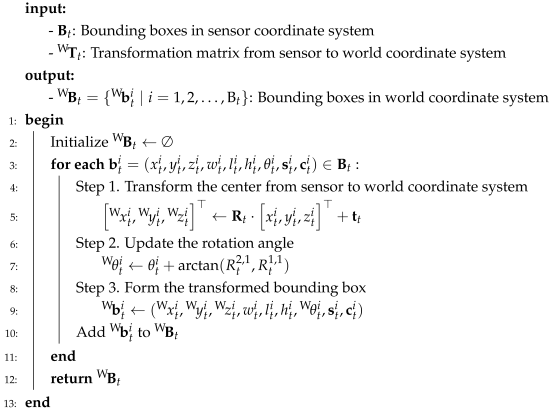
To experimentally evaluate the performance of LP-DSG, a Livox MID-360 (Livox, Shenzhen, China) LiDAR sensor is used as the low-density LiDAR, and a low-power NVIDIA Jetson AGX Orin (NVIDIA, Santa Clara, CA, USA) is employed to run the algorithm. The Livox MID-360 sensor can detect objects with 80% reflectivity at a maximum range of 70 m and objects with a reflectivity of 10% at a maximum range of 40 m. It also has a horizontal FOV of $360°$ and a vertical FOV that ranges from $-7°$ to $52°$. Sensor data is collected at 10 Hz intervals, with approximately 20,000 points per scan frame. The NVIDIA Jetson AGX Orin features an 8-core Cortex-A78AE CPU and an Ampere architecture-based GPU with 2048 CUDA cores, delivering up to 275 TOPS.

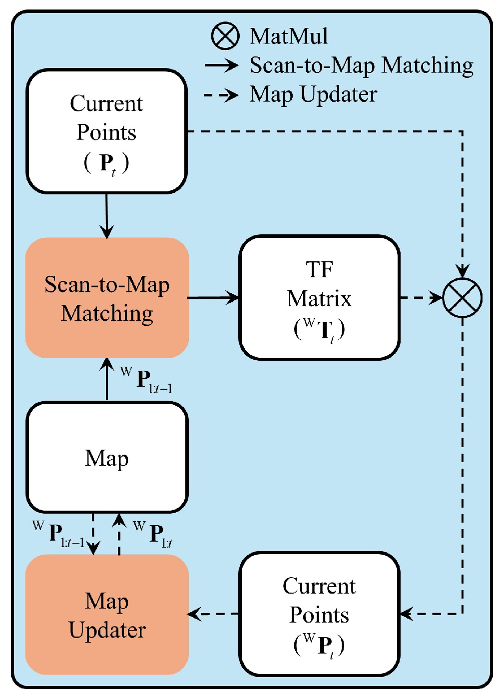
NDT is used as a scan-to-map matching technique. NDT partitions the point cloud into voxel spaces and models them as normal distributions, producing an optimal transformation matrix that minimizes the distributional differences between two LiDAR scans or between a LiDAR scan and a map. This process is used to generate the map. In LP-DSG, NDT is employed to match the LiDAR scans with the map to ensure stable map generation.

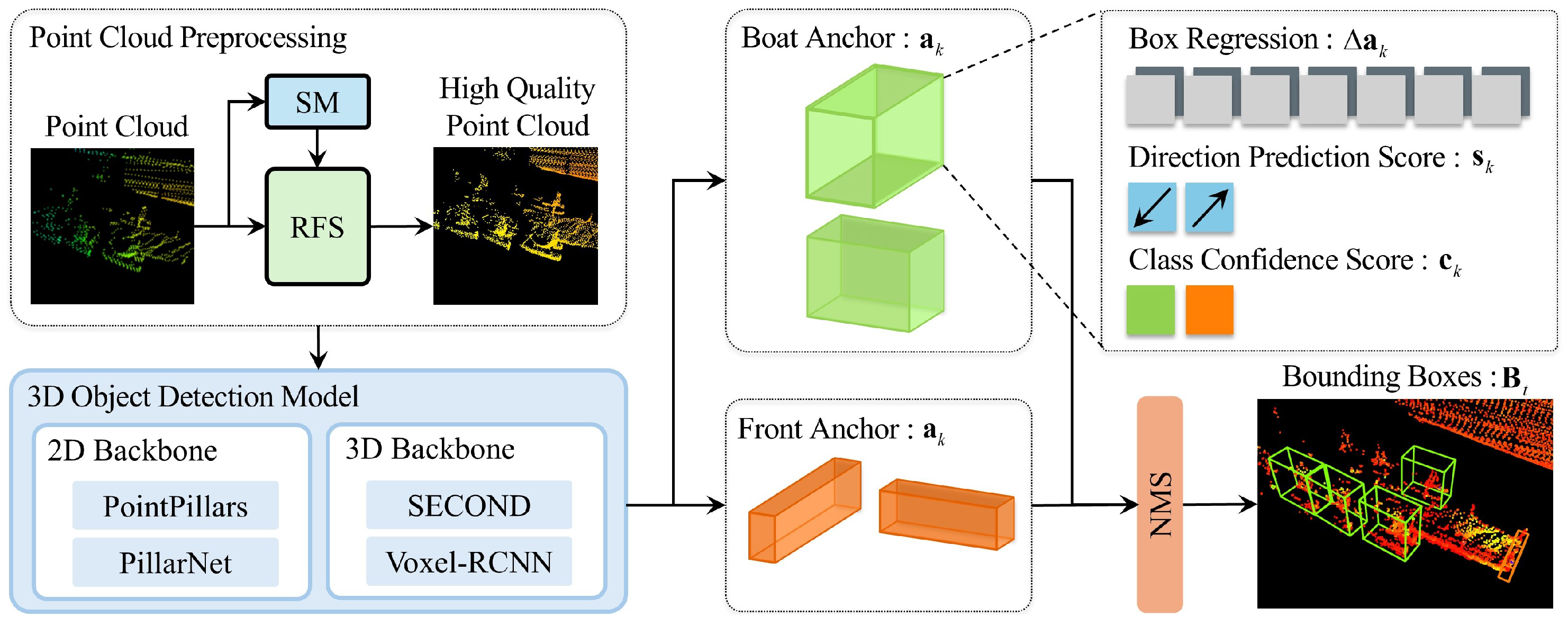
For 3D object detection, we used voxel-based PointPillars, PillarNet, SECOND and Voxel R-CNN models. Among these, PointPillars was selected as the experimental model for evaluating the entire LP-DSG system, including LOP and DSG algorithms, due to its computational efficiency suitable for real-time operation on embedded platforms while maintaining sufficient detection performance. For PointPillars, the voxel size $({\mathit{v}}_{\mathrm{X}},{\mathit{v}}_{\mathrm{Y}},{\mathit{v}}_{\mathrm{Z}})$ is set to (0.16, 0.16, 6) m, and each voxel is configured to hold a maximum of 16 points for computational efficiency. The point cloud queue size $\mathrm{Q}$ in Equation (6) is set to 5, determined through systematic experiments using this PointPillars configuration. 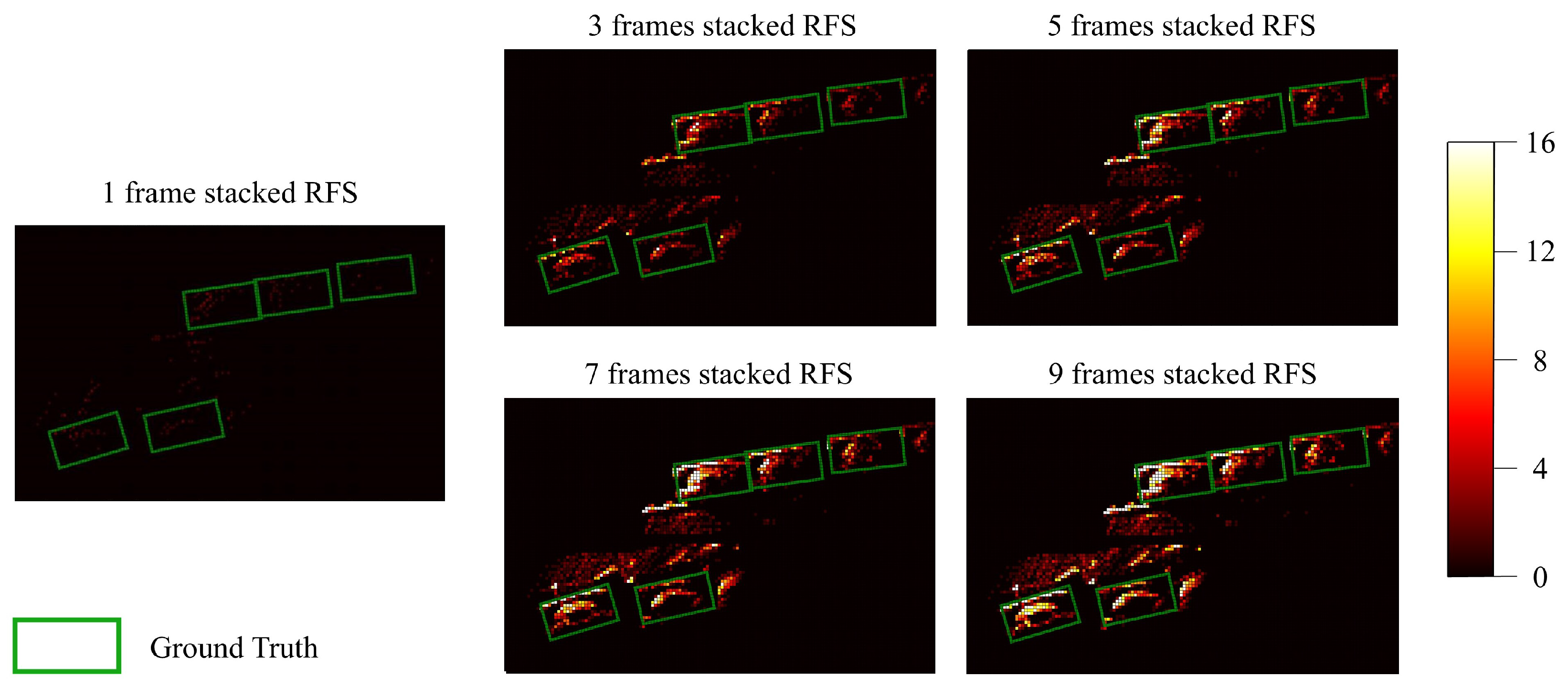Figure 8 visualizes the effect of different queue size $\mathrm{Q}$ on voxel occupancy as a heatmap, while

Table 1. Effect of queue size $\mathrm{Q}$ on voxel occupancy in ground truth bounding box region: The total number of voxels in the region is 1662.

Q	Voxel
	Empty	Non-Empty	Over-Capacity
1	1555	107	0
3	1227	435	5
5	1137	525	20
7	1074	588	61
9	1026	636	91

provides a detailed quantitative analysis. The analysis region contains 1662 voxels from the same ground truth bounding box.

As shown in Table 1, increasing $\mathrm{Q}$ from 3 to 5 adds 90 non-empty voxels while introducing only 15 over-capacity voxels, achieving a 6 to 1 ratio. However, further increasing from 5 to 7 adds just 63 non-empty voxels but introduces 41 over-capacity voxels, resulting in a 1.5 to 1 ratio. Here, non-empty voxels represent features that capture object geometry, while over-capacity voxels require random sampling that can disrupt learning. In PointPillars, when a voxel exceeds the 16-point limit, random sampling may produce point distributions that do not represent actual object surfaces, creating unrealistic geometric patterns that hinder model training. Additionally, larger queue sizes increase computational overhead, which can compromise real-time performance on embedded platforms. Therefore, $\mathrm{Q}$ of 5 was selected as the optimal balance that maximizes geometric feature coverage while minimizing both learning interference from random sampling artifacts and computational burden for real-time operation.

Furthermore, the ROI for USV $({\overleftrightarrow{x}}_{\mathrm{R}},{\overleftrightarrow{y}}_{\mathrm{R}},{\overleftrightarrow{z}}_{\mathrm{R}})$ is set to [−69.12, 69.12] m, [−69.12, 69.12] m, and [−2, 4] m, respectively, to enable detection in all directions. Voxel size $({\mathit{v}}_{\mathrm{X}},{\mathit{v}}_{\mathrm{Y}},{\mathit{v}}_{\mathrm{Z}})$ is determined with each model’s downsampling ratio in mind, as shown in

Table 2. Voxel size, feature map resolution, and downsampling ratio for each object detection model.

Model	Backbone	Voxel Size (m)	Feature Map Resolution	Downsample Ratio
PointPillars	2D	(0.16, 0.16, 6)	$432\times 432$	0.5
PillarNet		(0.08, 0.08, 6)	$216\times 216$	0.125
SECOND	3D	(0.16, 0.16, 0.15)	$108\times 108$	0.125
Voxel R-CNN		(0.16, 0.16, 0.15)	$108\times 108$	0.125

. Because 3D backbone models preserve detailed information along the Z-axis, reducing XY resolution incurs minimal performance loss. In contrast, 2D backbone models lose some Z-axis information when projecting to BEV and therefore require higher XY resolution to maintain a fine-grained representation. Accordingly, PillarNet uses a voxel size with half the XY dimensions of the other models to ensure sufficient performance despite its 0.125 downsampling ratio. The anchor sizes for the Boat and Front are set to (2.0, 3.8, 3.6) m and (3.6, 0.8, 1.5) m, respectively, reflecting actual object dimensions. All training-related settings, including network architecture, optimizer, scheduler, learning rate, and loss function, are implemented in OpenPCDet [44] using the default hyperparameter values specified in the original publications [35,37,40,41].

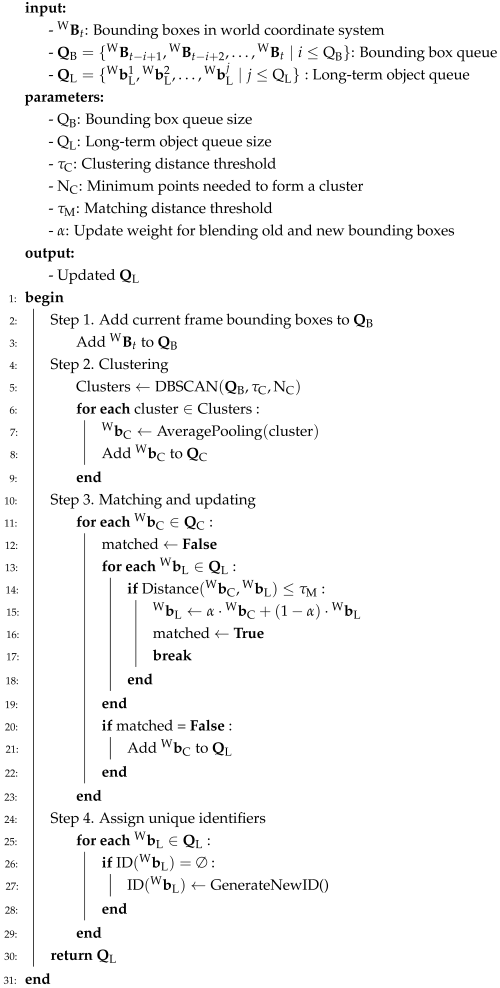
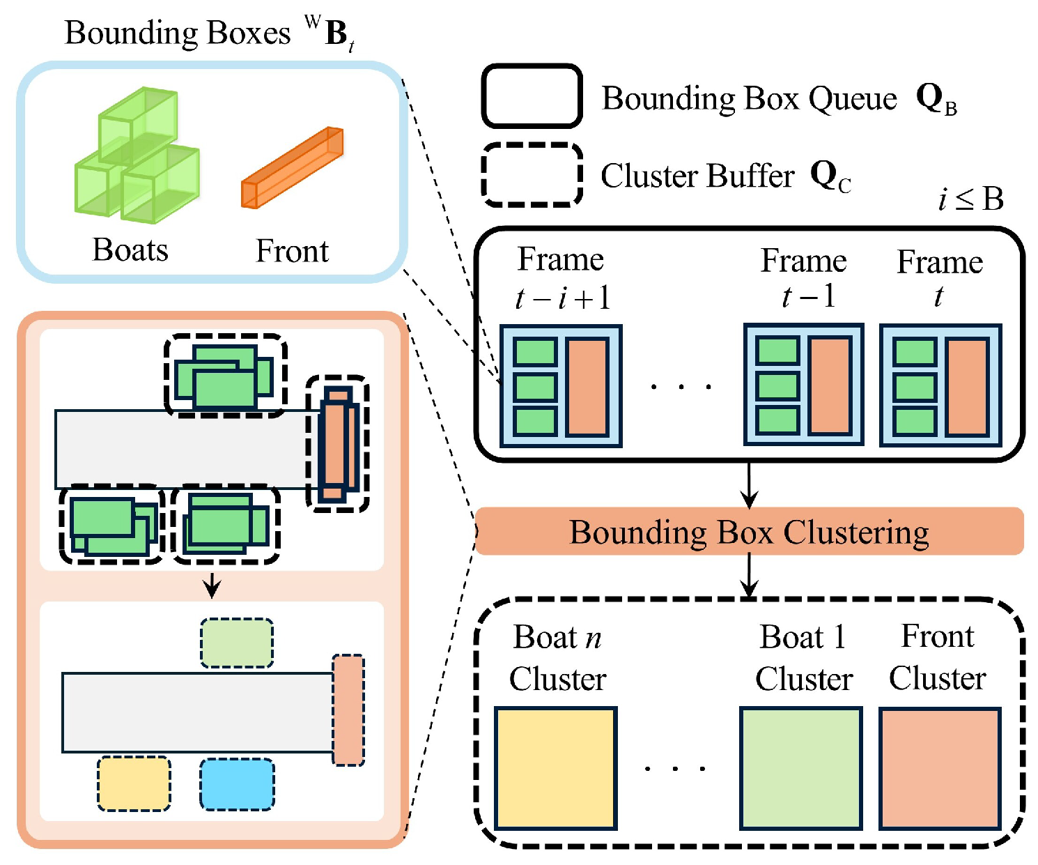
LOP employs DBSCAN as the clustering method. The DBSCAN parameters in Algorithm 2 are set considering the size of the USV, with the cluster distance threshold ${\tau }_{\mathrm{C}}$ set to 1.0 m and the minimum cluster points ${\mathrm{N}}_{\mathrm{C}}$ set to 3. 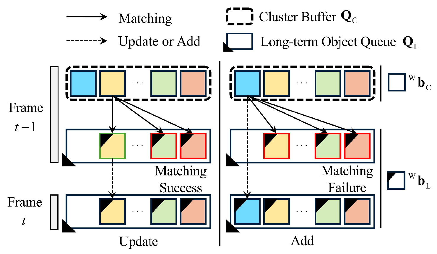Because LP-DSG operates across a relatively small scale of approximately 50 m, the sizes of the bounding box queue ${\mathrm{Q}}_{\mathrm{B}}$ and long-term object queue ${\mathrm{Q}}_{\mathrm{L}}$ are both set to 100, allowing up to 100 objects to be stored on the map. Considering the size of the USV and registration errors, matching distance threshold ${\tau }_{\mathrm{M}}$ between the cluster buffer and long-term object queue is set to 2.0 m. 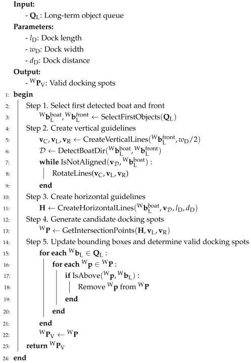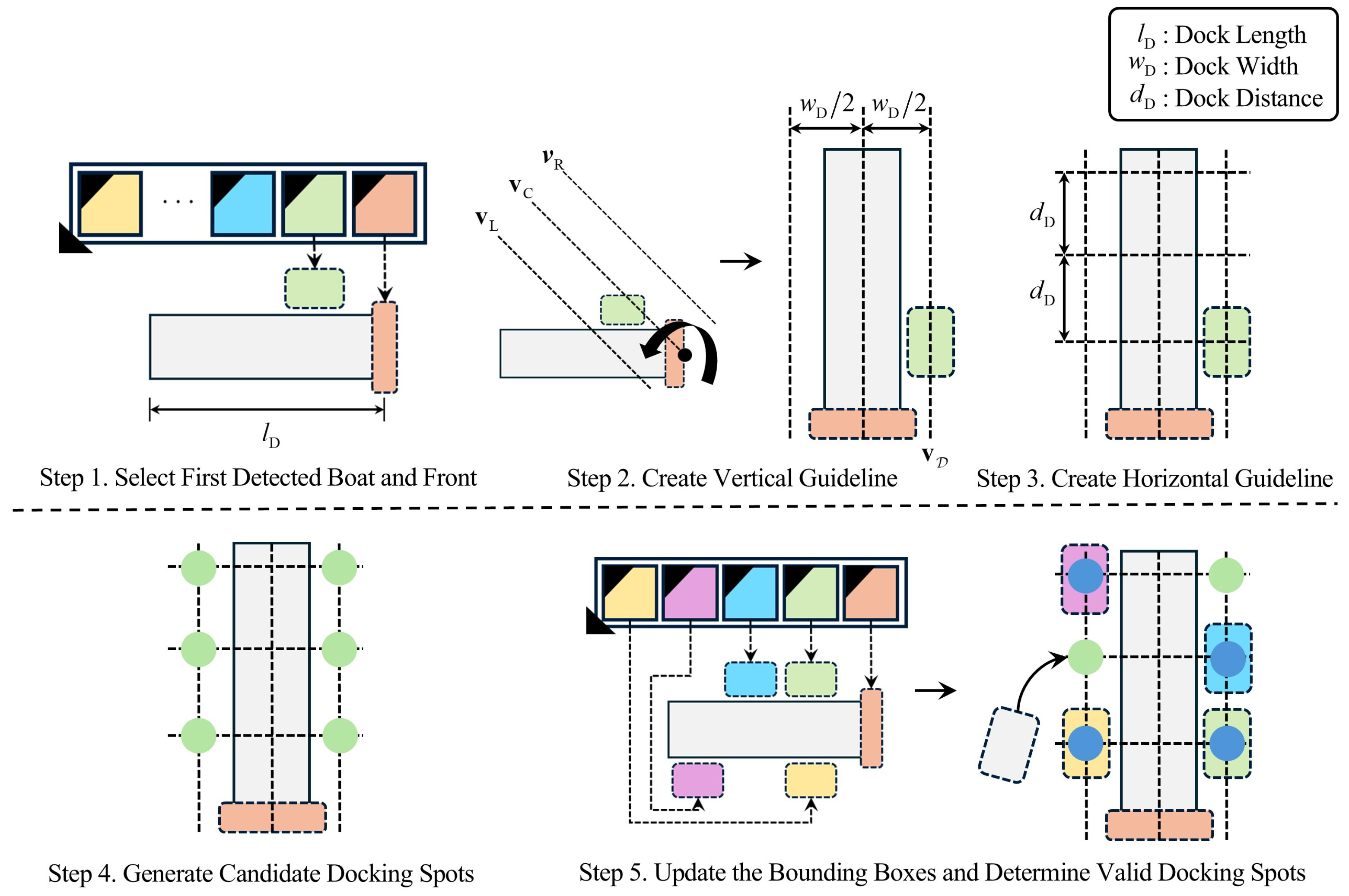Long-term object queue update weight $\alpha$ is set to 0.9, meaning that 90% of the information from the cluster buffer and 10% from the long-term object queue is incorporated to maintain the most up-to-date information during updates. 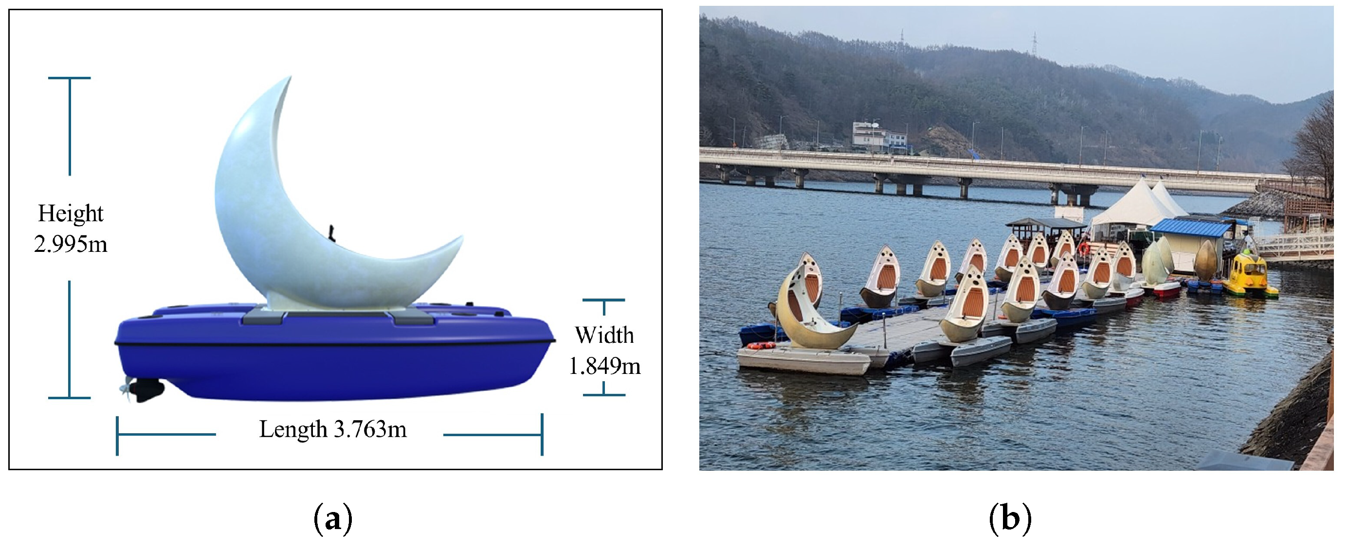Given the actual berthing environment for DSG, dock length $l_{\mathrm{D}}$ is set to 32.0 m, dock width ${\mathit{w}}_{\mathrm{D}}$ to 5.6 m, and dock distance $d_{\mathrm{D}}$ to 4.0 m. The specific dimensions for these parameters are derived from the physical constraints of the test site and the USV, as referenced in Figure 9a.

4.2. Dataset Construction

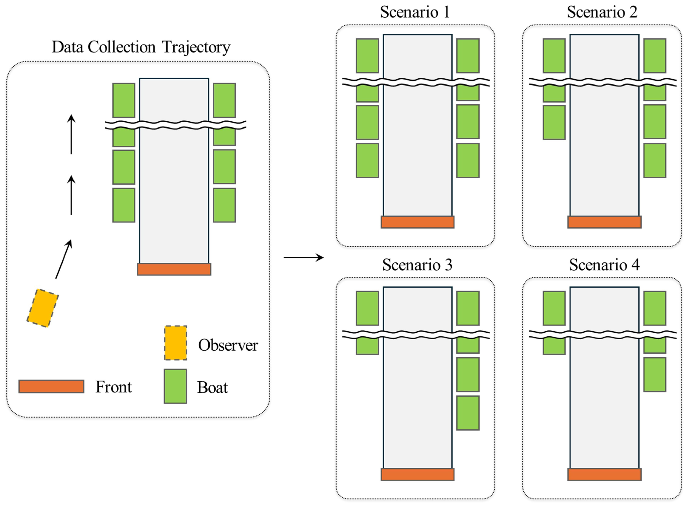
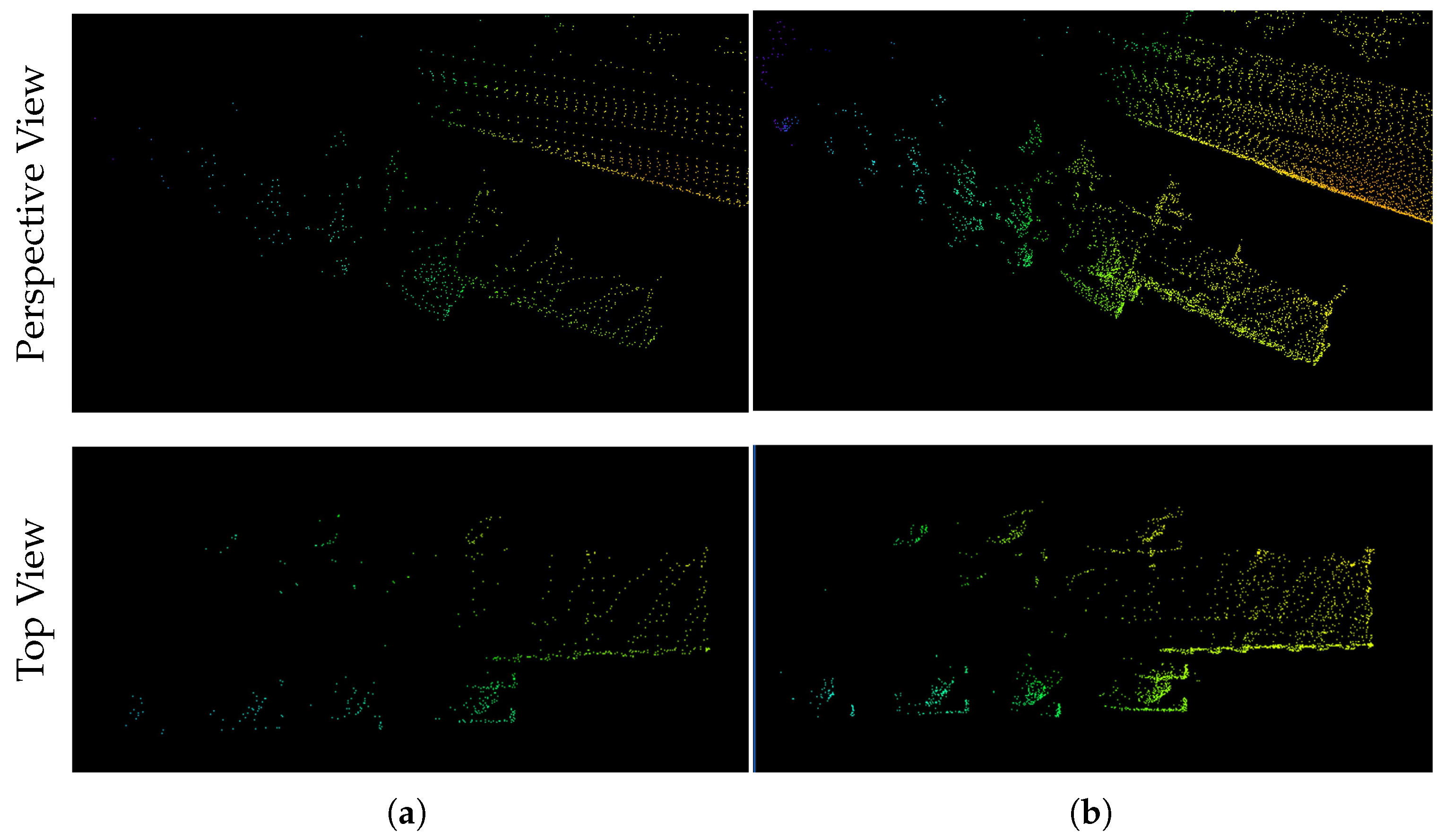
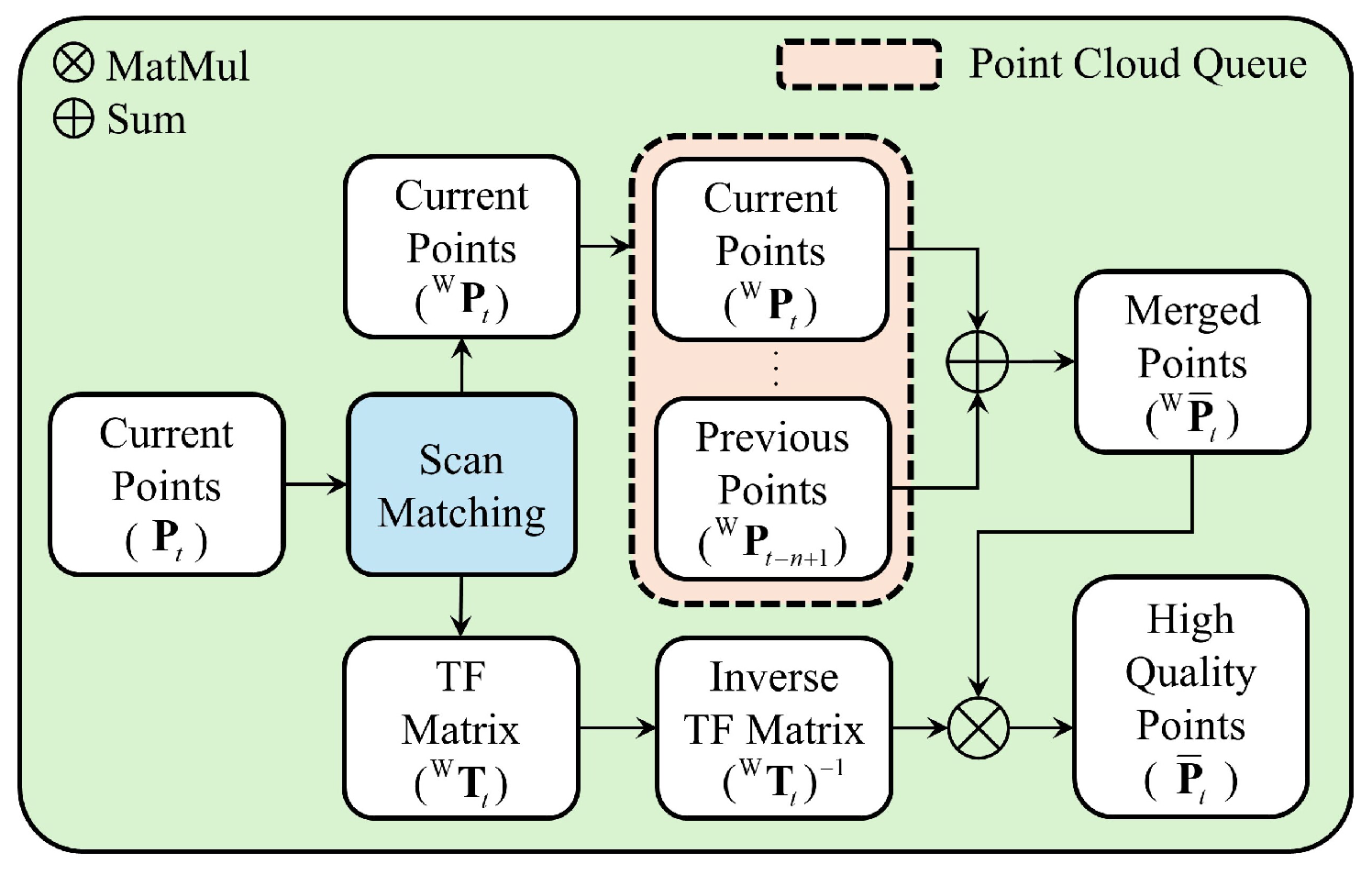
As shown in Figure 9b, the experiments are conducted on a large lake using a USV, from which the necessary data for training are collected. To ensure diversity in the point cloud data collected from LiDAR, three datasets were constructed based on four scenarios (Figure 10). The first dataset consists of raw point cloud data collected directly from LiDAR (Figure 11a), while the second dataset was generated by applying frame stacking (FS) to create high-quality point cloud data. FS accumulates point clouds from previous frames in the current frame to produce a merged point cloud, without a registration process. The third dataset was constructed by registering and merging five consecutive frames of raw point cloud data, producing high-quality point cloud data using RFS (Figure 11b).

All three datasets share the same label information, which was generated using the high-quality point clouds from RFS. This labeling approach is justified by the fact that all three datasets exist in the same sensor coordinate system and represent the same physical scenes captured at the same time. In LiDAR-based 3D object detection, bounding box annotations represent the physical dimensions and locations of objects based on surface points, independent of point density.

This follows the standard practice in major 3D detection benchmarks [17,42,45], where objects are labeled based on their physical extent regardless of point sparsity in any particular frame. Using consistent labels across all datasets ensures fair comparison by eliminating annotation variance as a confounding factor, allowing us to isolate and evaluate the effect of point cloud quality on detection performance. Each of the three datasets consists of the same 1722 scenes, and the labeled dataset is divided into 1378 and 344 scenes for training and validation, respectively.

We employ four data augmentation techniques to enhance training data diversity and reduce observation angle bias. First, we perform ground-truth sampling [37], which extracts points from labeled bounding boxes and inserts them into other scenes. We set the minimum points to sample to 5 for both Boat and Front classes, with up to 20 Boat objects and 5 Front objects inserted per scene. Second, we randomly flip each scene along the X and Y axes. Third, we apply random rotation around the Z axis within $(-\pi /4,\pi /4)$. Finally, we apply random scaling with factors between 0.95 and 1.05. These augmentations ensure that each training iteration encounters a different scene variation, allowing the model to learn from diverse inputs.

4.3. Experimental Results

Experiments are conducted to evaluate the improvement in object detection reliability and accuracy, efficiency in the long-term perception and management of objects, and the stability of DSG in real-world scenarios. In this experiment, PointPillars was selected as the experimental model for performing subsequent tasks after comparing object detection performance.

To evaluate the improvement in object detection reliability and accuracy due to the use of high-quality training data, a comparative analysis is conducted using 344 validation scenes, as shown in

Table 3. Object detection results.

Model	Method	3D AP@R40			BEV AP@R40
		Boat	Front	mAP	Boat	Front	mAP
PointPillars	Baseline	84.62	53.58	69.10	92.35	81.02	86.69
	+ FS	90.30	65.48	77.89	98.24	82.71	90.48
	+ RFS	93.64	89.45	91.55	96.45	99.78	98.12
PillarNet	Baseline	87.04	43.84	65.44	92.72	72.18	82.45
	+ FS	94.09	69.47	81.78	94.46	87.57	91.02
	+ RFS	94.36	83.03	88.70	94.49	99.66	97.08
SECOND	Baseline	80.15	36.82	58.49	89.29	66.02	77.66
	+ FS	90.58	56.53	73.56	93.81	80.53	87.17
	+ RFS	91.30	78.55	84.93	93.72	96.47	95.10
Voxel R-CNN	Baseline	92.27	56.89	74.58	95.26	77.18	86.22
	+ FS	99.01	82.33	90.67	99.23	93.44	96.34
	+ RFS	99.32	92.57	95.95	99.38	99.82	99.60

Gray shading indicates the proposed RFS method. Bold values represent the best performance across all methods for each metric.

. For each model, the evaluation compares its baseline and extended versions incorporating FS and RFS. Table 3 presents a quantitative evaluation of detection accuracy by comparing class-wise AP and mAP for both 3D bounding boxes and BEV. For all classes, the IoU threshold is set to 0.7, and 40 recall positions are used for a more detailed performance analysis [46,47].

As a result, compared to the single-frame baseline models, applying RFS consistently improves performance across all four model architectures. Quantitatively, RFS achieves an average 3D mAP improvement of 23.38 percentage points across all models. Specifically, PointPillars improves by 22.45 percentage points, PillarNet by 23.26 percentage points, SECOND by 26.44 percentage points, and Voxel R-CNN by 21.37 percentage points. Notably, the Front class shows particularly substantial improvements across all architectures. PointPillars achieves a 35.87 percentage point improvement, PillarNet 39.19 percentage points, SECOND 41.73 percentage points, and Voxel R-CNN 35.68 percentage points. These results indicate that high-quality point clouds generated by RFS are especially effective for detecting small objects with sparse point clouds. This consistent improvement pattern across diverse model architectures, ranging from lightweight PointPillars to complex Voxel R-CNN, validates the robustness and generalizability of our approach.

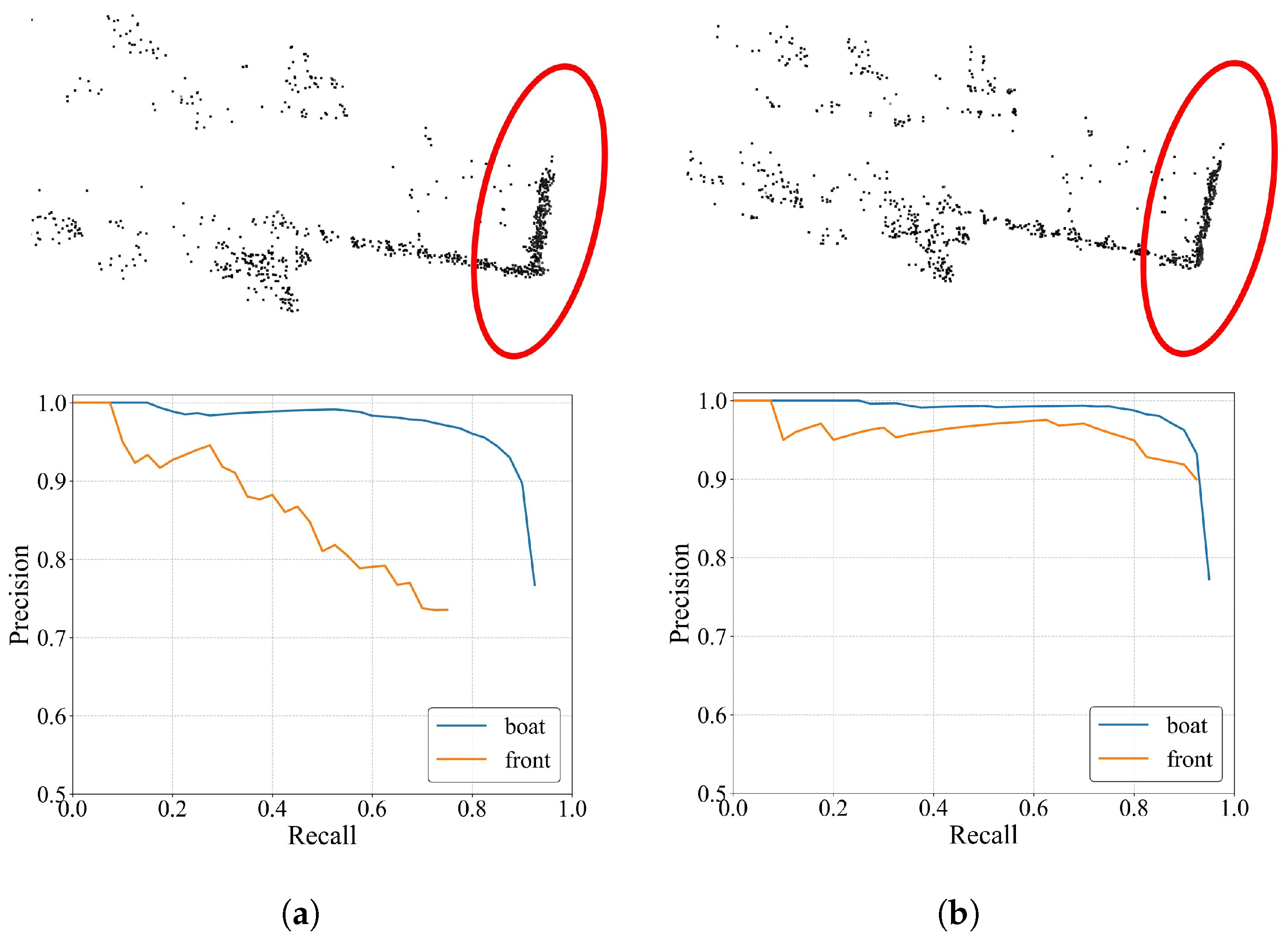
RFS produces a higher object detection performance than FS, another multi-frame model. This improvement is attributed to the multi-frame alignment process in RFS, which refines the point cloud, making it more suitable for object detection. Figure 12 visualizes the point cloud datasets generated by applying FS and RFS to the experimental model and shows the class-wise precision-recall (PR) curve results for each model. Notably, in the Front object region, indicated by the red ellipse, the FS data sample produces an unstable object shape. In contrast, with RFS, the object shape is more stable due to precise frame alignment. This is a critical factor in detecting relatively small objects such as the Front.

Figure 13 presents the inference results for the experimental model. Compared to the ground truth, the baseline and baseline with FS models (Figure 13a and Figure 13b, respectively) fail to detect the Front, while the baseline with RFS model reliably does so (Figure 13c).

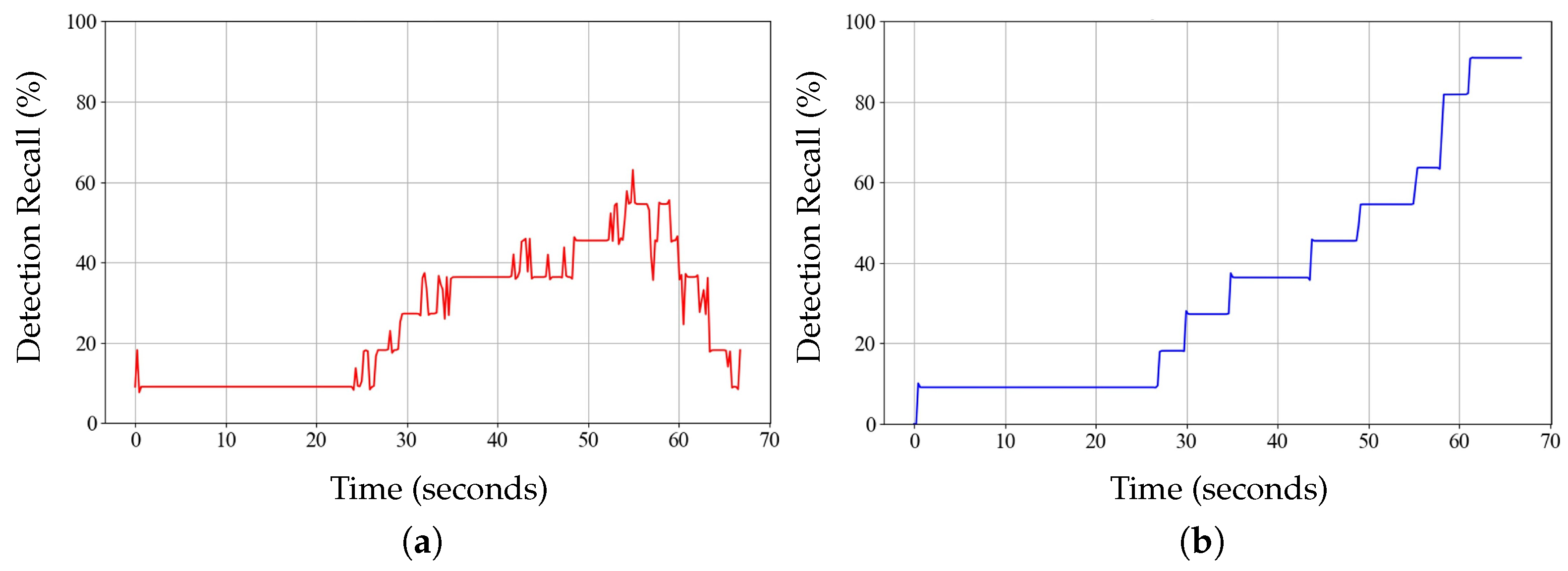
To evaluate the effectiveness of long-term perception and object management, we compare the detection recall (DR) with and without LOP. Figure 14 presents the DR over time, representing the detected objects as a percentage of the total number of actual objects in Scenario 3 of Figure 10. When LOP is not employed, the DR gradually increases over time but starts to decline after reaching 60% (Figure 14a). This decline can be attributed to objects moving out of the LiDAR FOV. In addition, due to noise in the real-world environment, the DR fluctuates during the detection process. In contrast, when LOP is used, the DR steadily increases over time (Figure 14b). This is because LOP retains object information even when they move out of the LiDAR FOV. As a result, a DR of approximately 90% is achieved in Scenario 3, contributing to the stability of DSG.

The stability of the DSG algorithm employed in Scenario 1 of Figure 10 is also tested.

Table 4. DSG results.

Model	Matching Distance (m)
	Avg.	Std. Dev.	95% CI
Baseline	0.654	0.125	[0.614, 0.693]
+ RFS	0.579	0.152	[0.531, 0.627]

Gray shading indicates the proposed RFS method. Bold values represent the best performance for each metric.

presents the DSG results for the baseline and RFS of the experimental model. Nearest-neighbor matching is performed in the XY plane between the bounding boxes of the Boat stored in LOP and the candidate docking spots generated by the DSG algorithm. The mean, standard deviation, and 95% confidence interval of the matching distances between paired points are calculated. As a result, the baseline model exhibits a mean matching distance of 0.654 m, whereas the model with RFS achieves an improved mean matching distance of 0.579 m. Additionally, when comparing the confidence intervals of both models, the baseline model has a range of [0.614, 0.693] m, while the model with RFS has a range of [0.531, 0.627] m. Because the confidence interval widths are relatively small compared to the size of the USV, which has a length of 3.8 m and a width of 1.8 m, it can be confirmed that the DSG algorithm is stable in both cases. 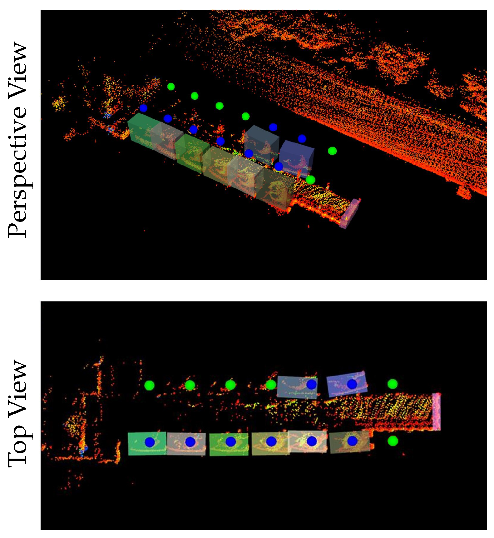Figure 15 visualizes the DSG results for the model with RFS, confirming that the system can reliably generate autonomous docking spots in real-world environments. A detailed visualization of the complete LP-DSG system workflow is provided in Video S1.

5. Discussion and Conclusions

In the present study, we proposed LP-DSG, a LiDAR point-based docking spot generation system for autonomous USV docking using low-density LiDAR in berthing environments. The key innovation of LP-DSG is the integration of scan matching with registration-based frame stacking (RFS) to generate high-quality point clouds from low-density LiDAR data. This approach enables accurate object detection and long-term environmental perception, which are essential for reliable autonomous docking spot generation.

To validate the performance of LP-DSG, we conducted experiments in a large lake using a USV. The USV was equipped with low-density LiDAR and an embedded board, and its performance was evaluated under practical operating scenarios. Based on the experimental results, the proposed approach was shown to be effective in improving the accuracy of 3D object detection, the long-term perception and management of objects, and the stability of DSG. Given its practical applicability in real-world environments, LP-DSG is thus suitable for low-density LiDAR. In particular, it has the potential to be a cost-effective alternative for situations where the use of expensive high-precision sensors may not be feasible, such as with small autonomous vessels, USVs, and floating offshore structures.

While LP-DSG demonstrates effective performance in berthing environments, several limitations should be acknowledged. One limitation is that the RFS method inherently accumulates points from sequential frames over time, which limits its applicability in highly dynamic environments. When objects in the scene move significantly between frames, the point cloud registration process may introduce misalignment artifacts, potentially degrading the quality of the accumulated point cloud. Our current implementation is therefore most suitable for berthing scenarios where the environment is relatively static.

Another limitation is that the DSG algorithm relies on the successful detection of both Front and Boat objects stored in long-term object queue. The Front serves as a landmark for establishing the global coordinate system and generating guidelines, while the Boat provides directional information for determining docking orientation. If either object fails to be detected due to occlusion, sensor limitations, or challenging environmental conditions, the system cannot generate optimally oriented docking spots. However, we note that if only the Front is detected, it would be possible to generate docking spots using the Front’s orientation information as a default docking direction, though this would result in less accurate directional alignment compared to using actual Boat positions. This dependency on landmark detection represents a fundamental limitation of the current approach.