Lightweight Multi-Class Autoencoder Model for Malicious Traffic Detection in Private 5G Networks

Abstract

This study proposes a lightweight autoencoder-based detection framework for the efficient detection of multi-class malicious traffic within a private 5G network slicing environment. Conventional deep learning-based detection approaches encounter difficulties in real-time processing and edge environment applications because of their significant computational complexity and resource demands. To address this issue, this study balances traffic data using slice-label-based hierarchical sampling and performs domain-specific feature grouping to reflect semantic similarity. Independent autoencoders are trained for each group, and the latent vectors from the encoder outputs are combined to be used as input for an SVM-based multi-class classifier. This structure reflects traffic differences between slices while also improving computational efficiency. Four sets of experiments were constructed to verify the model’s performance and evaluate its structural performance, resource usage efficiency, classifier generalization performance, and whether it met SLA constraints from various perspectives. As a result, the proposed Multi-AE model achieved an accuracy of 0.93, a balanced accuracy of 0.93, and an ECE of 0.03, demonstrating high stability and detection reliability. Regarding resource utilization efficiency, GPU utilization was under 7%, and the average memory usage was approximately 5.7 GB, demonstrating resource efficiency. In SLA verification, inference latency below 10 ms and a throughput of 564 samples/s were achieved based on URLLC. This study is significant in that it experimentally demonstrated a detection structure that achieves a balance of accuracy, lightweight design, and real-time performance in a 5G slicing environment.

1. Introduction

In recent years, detection of malicious traffic using AI has emerged as one of the most actively researched areas within network security [1]. Conventional signature-based or rule-based detection systems, which depend on static policies, have difficulty addressing contemporary cyber threats that are always developing and evading detection [2,3,4]. Accordingly, machine learning and deep learning-based intrusion detection systems (IDSs) are attracting interest as pattern-oriented methodologies capable of learning from extensive traffic data, comprehending intricate patterns, and identifying previously undiscovered threats.

With the spread of private 5G networks, the importance of malicious traffic detection is becoming even more prominent. Private 5G networks are used in enterprise or industrial environments and have a multi-logical network slice structure to support various service types, such as enhanced mobile broadband (eMBB), ultra-reliable low-latency communication (URLLC), and massive machine-type communication (mMTC) [5,6]. Each slice enhances efficiency and flexibility by providing independent resources and quality of service (QoS). Attackers can exploit the fact that if traffic for each slice is handled through separate virtual networks, the central control system will find it difficult to directly observe detailed packet flows [7]. By manipulating control signals or resource management mechanisms between slices, they can cause service disruption or performance degradation [8]. In particular, slice operation is performed based on a Service Level Agreement (SLA) defined by latency, throughput, resource utilization, and so on [9]. These indicators go beyond simple quality assurance standards and can be interpreted as crucial security signals that allow for the early identification of anomalous behavior. Therefore, malicious traffic detection in a 5G slice environment requires not only high accuracy but also lightweight performance and real-time capabilities to maintain SLAs. However, most existing studies are limited by the fact that they are trained based on large-scale supervised learning in a single network environment or by treating all traffic features in the same way, failing to fully reflect the structural differences between 5G slices. Furthermore, complex deep learning models are difficult to apply in edge devices or distributed environments at the slice level due to their high computational cost [10,11].

Against this backdrop, this study proposes a lightweight, autoencoder-based AI traffic detection model in a private 5G network environment. The proposed model normalizes traffic data through multi-stage preprocessing and then separates semantically similar features into domain groups, training an autoencoder for each group. Subsequently, by combining the latent vectors of each encoder and training a multi-class classifier based on Support Vector Machine (SVM) [12] various attack types between 5G slices are efficiently detected. This structure reduces associative complexity while simultaneously preserving feature interactions and pattern differences between slices, thereby improving real-time processing performance. Ultimately, this study aims to lighten the burden of AI-based malicious traffic detection in a 5G slicing environment while maintaining accuracy. Specifically, this study proposes a new detection framework that combines feature compression using an autoencoder with an SVM-based multi-classification structure, enabling both real-time detection and generalized attack identification.

The main contributions of this study are as follows.

• Suggestion of a Slice-Aware Data Preprocessing Structure: A hierarchical, balanced sampling procedure is designed by simultaneously considering slices and labels to mitigate the data imbalance problem that occurs in 5G network slicing environments.
• Systematization of Domain-Based Feature Grouping and Preprocessing: Data correlation and stability are ensured by classifying traffic features into 6 domain groups based on semantic similarity and performing preprocessing steps for each group.
• Suggestion of a Group-wise Autoencoder Learning Structure: Group-specific variability is preserved by applying independent autoencoders to each feature group. For groups containing slice information, a slice identifier is added as an input to learn the traffic differences between slices.
• Design of a Lightweight SVM-based Multi-class Detection Structure: By combining only the encoders of the group-wise autoencoders and using the latent representation as input to train an SVM classifier, an efficient detection architecture is implemented that maintains high detection performance while reducing computational cost.

This paper is organized as follows. Section 2 introduces the theoretical background of Private 5G Networks, Network Slicing, SLAs, and Autoencoders. Section 3 examines related studies and discusses the limitations of conventional methodologies. Section 4 outlines the overall structure and step-by-step methodology of the proposed detection framework. Section 5 assesses the proposed model’s detection performance and efficiency using experimental conditions and outcomes. Finally, Section 6 draws conclusions and suggests future research directions and scalability.

2. Background

2.1. Private 5G Network & 5G Network Slicing

Private 5G networks are a popular technology for industrial applications, offering solutions for edge computing, but current implementation methods can be expensive and complex for simpler scenarios [13]. Network slicing is an important technology that makes it possible for new services and solutions to work in 5G and future 6G communications [14,15,16]. This technology allows Mobile Network Operators (MNOs) to deploy multiple logical and independent networks on top of their physical infrastructure, with each network orchestrated according to specific service requirements [17]. These logical slicing networks can be managed and configured individually based on various parameters, such as bandwidth, latency, privacy, and QoS. The ultimate goal of 5G network slicing is to achieve end-to-end (E2E) network slices that span from the mobile edge, through mobile transport, and into the core network. E2E network slicing presents various design challenges and requires advanced management and automation. Key enabling technologies for network slicing include Network Function Virtualization [18]. Both optical network virtualization and network slicing are important enabling technologies for future 5G networks [19].

2.2. SLA (Service Level Agreement) in 5G Network Slicing

SLA in 5G network slicing defines the QoS and performance levels that each slice must guarantee [20,21]. It requires agreements between network operators and service providers, specifying measurable key performance indicators (KPIs) to ensure independent performance for each slice, such as latency, throughput, reliability, and availability [22]. SLA defines different quality conditions based on the service characteristics of each slice and enables independent operation without interference between slices [23].

In 5G, the following three representative slice types are defined based on service purpose [24].

• eMBB (enhanced Mobile Broadband): The eMBB slice is designed for high-volume content delivery and ultra-fast data services. It is optimized for bandwidth-intensive services used by general consumers, such as mobile internet, cloud streaming, and high-definition video calls. This slice primarily ensures high throughput and session persistence, requiring stable connections even when users move. Additionally, multiple access control (MAC) and dynamic scheduling techniques are applied to minimize QoS degradation even in high-traffic environments. The core parameters of the eMBB SLA are high throughput and session continuity, which are designed to maximize bandwidth efficiency [25].
• URLLC (Ultra-Reliable Low-Latency Communication): URLLC slices are specialized for real-time control-based services that require ultra-low latency and high reliability. It is applied to mission-critical services such as vehicle-to-everything (V2X) communication for autonomous vehicles, robot control in smart factories, and remote surgery [26]. Because the SLA for URLLC slices is extremely sensitive to packet loss and jitter, the network guarantees deterministic performance through resource reservation and route isolation. Furthermore, it is designed to minimize the probability of service interruption by combining reliability enhancement technologies such as Multipath TCP (MPTCP) and Hybrid ARQ retransmission control [27].
• mIoT (Massive Internet of Things): The mIoT slice is designed for environments where a massive number of IoT devices connect simultaneously, focusing on low power, low bandwidth, and massive connectivity. It is mainly suitable for services that focus on periodic data collection or status reporting, such as smart metering, sensor networks, and environmental monitoring. The SLA for this slice focuses on ensuring connectivity stability and UE density rather than latency, efficiently allocating network resources to allow hundreds of thousands of devices to communicate stably within a single cell [28]. Designed for long-term operation by optimizing transmission cycles and energy efficiency, this protocol maximizes operational efficiency in large-scale IoT infrastructure [29,30].

The SLA requirements for each slice type are summarized in

Table 1. Summary of SLA and QoS Indicators for 5G Network Slice Types.

Slice Type	QoS Profile (5QI Example)	Latency Limit (ms)	Packet Error Rate	Priority	Example Services
eMBB	1, 2, 5–9	100–300	1%–10−6	10–90	Video Streaming, Voice/Video Calls, Cloud Service
URLLC	82	≥10	0.01%	19	Autonomous driving, Industrial robot control, Remote Surgery
mIoT	9	300	10−4–10−6	90	Smart metering, Sensor networks, Environmental monitoring

[5,6].

(Standards-Based SLA Benchmarks) While Table 1 reflects the KPI profiles and service-quality indicators defined in GSMA NG.116 [5], slice-specific SLA benchmarks are also explicitly defined in 3GPP specifications. 3GPP TS 28.530 [31] and TS 28.531 [32] introduce the network slice SLA-management architecture, defining service profiles, service-level specifications (SLSs), measurement procedures, and assurance functions. In addition, 3GPP TS 28.541 [33] provides a detailed list of standardized performance indicators such as guaranteed bitrate (GBR), maximum packet delay budget, jitter constraints, and packet error rate thresholds that must be satisfied for slice assurance. This study aligns with both frameworks:

• GSMA NG.116: Table 1 and QoS/KPI mappings (operator-oriented SLA baseline)
• 3GPP TS 28.530/28.531/28.541 [31,32,33]: Technical SLA benchmarks and monitoring requirements

By grounding our evaluation in these standardized SLA definitions, the performance metrics analyzed in this work—latency, throughput, reliability, and resource efficiency—directly correspond to the slice-specific benchmarks defined by key standardization bodies.

2.3. Autoencoder

Autoencoder (AE) is an unsupervised learning-based neural network that learns the intrinsic structure of data by compressing input data into a low-dimensional latent space and then reconstructing it back to its original form, as shown in Figure 1 [34].

This model consists of two main components.

• Encoder: Encodes input data into a latent representation to extract key features.
• Decoder: Reconstructs the original input from the encoded representation.

The learning objective of an autoencoder is to minimize the difference between the input vector $x$ and the reconstructed vector $\widehat{x}$. Generally, Mean Squared Error (MSE) is used as the loss function, and it is defined as follows:

$$L\left(x, \widehat{x}\right)={\displaystyle \frac{1}{n}}{\parallel x-\widehat{x}\parallel }^2$$

(1)

In this process, the model learns the distributional characteristics of the input data on its own, acquiring the ability to remove unnecessary noise and compress only the important features. In particular, the reconstruction error can be used as an indicator to distinguish between normal and anomalous data [35]. Autoencoders go beyond simple dimensionality reduction techniques and are applied in various fields such as anomaly detection, data compression, and denoising. In the field of network security, models trained on normal traffic are effectively used for intrusion detection (IDS) and anomaly detection by exploiting the fact that they exhibit high reconstruction errors for abnormal patterns. Furthermore, autoencoders can be utilized in security data environments where labels are scarce, playing a significant role in network threat detection research based on unsupervised or semi-supervised learning.

In 5G networks and cybersecurity environments, autoencoder-based approaches offer higher efficiency and adaptability compared to simple statistical detection methods due to the high dimensionality and irregularity of traffic data. This enables various applications such as real-time anomaly detection, network slicing-based traffic analysis, and identification of DDoS and session-based attacks. Importantly, lightweight autoencoder models can be applied even on network terminals or edge devices, allowing for expansion into a distributed detection architecture.

3. Related Works

3.1. Autoencoder Based Attack Detection

Salahuddin et al. [36] proposed Chronos, a time series-based anomaly detection system that efficiently detects DDoS traffic using an autoencoder that leverages time-based features over multiple time periods. This system improved performance against various DDoS attacks by developing a heuristic that selects the threshold that maximizes the F1 score. This study achieves performance that is slightly superior to other time series-based systems while using a less complex anomaly detection pipeline, and it outperforms flow-based approaches with greater precision. Additionally, they claim suitability by demonstrating robustness despite zero-day attacks, noise in the training data, and a small number of training packets.

Catak et al. [37] point out the limitations of most current approaches, which are based on supervised learning that requires large, balanced datasets and struggles to identify new types of attacks. To address these limitations, they proposed a semi-supervised DDoS detection model using autoencoders and SVMs. This model achieved 99.57% accuracy and over 99% precision, recall, and F1-score on the CICDDoS2019 dataset, outperforming other models.

Salahuddin et al. [38] note that DDoS attacks continue to receive significant attention due to the surge in cyberattacks targeting the healthcare, education, and financial sectors during the COVID-19 pandemic. The expansion of virtualization and software-defined technologies, along with the surge in IoT devices, is increasing the attack surface and the impact of network attacks. This study presents a novel time series-based anomaly detection system utilizing an autoencoder and investigates its various impacts on detecting several DDoS attacks that are difficult to detect with flow-based features. The proposed approach was trained and evaluated on the CICDDoS2019 dataset, achieving F1-scores of over 99% for most attacks and over 95% for all attacks.

3.2. Real-Time-Based Network Attack Detection

Shi et al. [39] argue that most DDoS attack detection methods proposed in the past have limitations in that they rarely consider real-time performance, adaptability, and other practical issues in real network environments. This paper proposes RT-SAD (Real-Time Sketch-Based Adaptive DDoS Detection), a real-time adaptive DDoS attack detection method based on external network responses when an attack occurs. RT-SAD was designed to be suitable for high-speed network environments by developing a sketch-based feature extraction method and an adaptive update algorithm. The experimental results indicated that this method could detect DDoS attacks in high-speed network environments using sampled Netflow data, and it exhibited excellent real-time performance, low resource consumption, and high accuracy.

Tang [40] states that traditional convolutional neural networks (CNNs) have limitations, requiring more advantages in real-time network intrusion processing. This paper proposes a novel detection method using visualization techniques when real-time traffic data is missing. The system uses offline data to digitize and pixelate hacked network traffic, then performs grayscale conversion as a preprocessing step. This data is rotated to the right and connected to the CNN interface for training. The proposed model was validated using real-time network data and demonstrated excellent detection performance, proving its ability to detect real-time network intrusion types.

3.3. AI-Based Security in 5G Network Slicing

Dangi et al. [41] aimed to address the limitations that, while 5G network slicing is crucial for meeting diverse service requirements, the associated security issues necessitate comprehensive exploration and analysis, and there was a lack of studies that comprehensively compared the machine learning-based approaches presented in existing literature. Their study thoroughly examines machine learning methodologies within 5G network slicing contexts by identifying and categorizing them. Additionally, it explains the concept, layers, and architectural framework of 5G Network Slicing; discusses attacks, threats, and prevention of issues; presents a classification scheme compared to existing research; and demonstrates that models such as machine learning-based, reinforcement learning, CNN, multi-agent reinforcement learning, and distributed SVM are effective in enhancing security.

Thantharate et al. [42] claim that it is vital to maintain the isolation of resources, traffic flows, and network functions between slices for protecting network infrastructure systems from threats like DDoS attacks in a 5G network environment. Therefore, their study develops a neural network-based “Secure5G” network slicing model that proactively detects and removes threats based on incoming connections before they can infect the 5G core network. This model is a neural network-based deep learning framework that provides end-to-end security for 5G networks and addresses the limitations of traditional security approaches by proactively detecting and isolating threats.

3.4. Attack on 5G Network

Singh et al. [43] argue that traditional security tactics (e.g., static security, single points of failure) are inadequate for identifying attacks based on the dynamic nature of 5G networks and addresses issues such as slice isolation, authentication, and authorization. To address these issues, they deeply analyze security vulnerabilities affecting various aspects of 5G network slicing implementation and management, identify the five most vulnerable areas within slicing, and propose security methods.

Olimid et al. [44] conducted an in-depth investigation into 5G network slicing, focusing on a structural framework, applications, service variations, security considerations, and an extensive review of existing literature. Their study addresses vulnerabilities and potential threats that pose risks to 5G network slicing. It also comprehensively investigates various types of potential attacks, revealing the security challenges inherent in this paradigm.

Dias et al. [45] explore the security issues associated with network slicing in 5G networks, a technology that allows for the creation of virtual networks tailored to various use cases. Their study contributes to network slicing research by providing a comprehensive classification of attacks aligned with the 5G architecture layers and complementing practical mitigation approaches suitable for multi-tenant environments. The proposed classification aims to categorize specific attacks and vulnerabilities across layers such as orchestration, virtualization, and inter-slice communication. Mitigation strategies are also discussed, emphasizing the importance of real-time monitoring and access control.

Lee et al. [46] state that 5G wireless networks offer ubiquitous internet access, high user, and device mobility, and IoT device connectivity, but they also present new challenges related to the secure implementation of these technologies and the provision of user privacy. In particular, advancements in cloud computing, Software Defined Networking (SDN), and Network Functions Virtualization (NFV) introduce new security vulnerabilities. Their study investigates user equipment privacy and security issues in 5G networks and presents technologies to address these problems.

4. Methodology

4.1. Architecture

The goal of this study is to maintain multi-class attack detection performance while meeting real-time processing requirements (latency, throughput, resource constraints) in a 5G network slicing environment. The proposed methodology consists of four steps, as shown in Figure 2.

(1) Data diversity and balance are ensured through hierarchical sampling at the slice and label levels. (2) To protect personal information and prevent overfitting, sensitive features are excluded, the remaining features are grouped based on meaning, and slice information is integrated into groups associated with slices. Afterward, preprocessing is performed for each group in the order of winsorize, imputate, and standardscalar to maintain data correlation and consistency. (3) After training an autoencoder for each feature group, only the encoder part is extracted and the multi-dimensional features are compressed into a low-dimensional latent space, thereby reducing the computational complexity during classification. (4) The encoder output vectors for each group are integrated and used to train and infer with an SVM-based multi-class classifier. This architecture ensures detection accuracy while maintaining interactions between slices of features, simultaneously improving throughput and memory efficiency.

4.2. Sampling of the Dataset

This study systematically designs a data sampling process to balance the learning of various attack types in a 5G network slicing environment. The network traffic data includes slice identifiers and is collected into two slices (slice 1 and 2), with each sample consisting of statistical features of traffic flow units and their corresponding labels. However, actual 5G traffic tends to be unevenly distributed depending on the service characteristics of each slice and the frequency of attacks. This data imbalance can distort the learning performance of classifiers, leading to overfitting and reducing detection sensitivity for the minority class. Therefore, this section applies to a slice-label-based hierarchical stratified balanced sampling technique.

Since 5G traffic data is collected on a large scale, using the entire dataset directly for training is inefficient in terms of computational efficiency and training time. Therefore, to construct samples of a size suitable for model training while maintaining the representativeness and diversity of the data, the data is extracted in a balanced manner based on slice and label distributions. The sampling process is performed in two stages. (1) In the distribution exploration phase, the data distribution is analyzed for each slice and label combination. Determine the sample size for each combination and verify that sufficient data has been obtained. (2) In the balanced collection step, random sampling based on random numbers is performed to ensure that each slice-label combination is equally reflected in the learning process. This reduces data bias and ensures that all attack types contribute equally to learning. Combinations with excessive data are adjusted through down sampling, and minority classes are added evenly.

The sampled data is divided into three sets: Train, Validation, and Test. The stratified split method is applied to each set to maintain a consistent class distribution. When splitting, the random number seed is fixed to ensure reproducibility. This data-splitting structure is reflected equally across all classes.

The final dataset constructed is designed to include some attack types and normal traffic evenly across the two slices. Each slice maintains different traffic characteristics while sharing the same feature space, allowing the model to learn detection capabilities that are mutually independent between slices. This slice-label-based hierarchical sampling technique simultaneously ensures data diversity and balance, achieving generalized detection performance without bias toward specific classes in subsequent autoencoder-based dimensionality reduction and SVM classification processes.

4.3. Preprocessing

In the data preprocessing stage, a data preprocessing procedure was configured to mitigate the imbalance and noise issues in 5G network traffic and to ensure the stability and generalization performance of model training. The preprocessing process consists of five steps: (1) Attack Grouping, (2) Feature Grouping, (3) Winsorization, (4) Imputation, (5) Standardization by Group, and (6) Class Balancing. Each step aims to improve data quality and prevent the model from being biased toward specific classes or features.

(1)

In the Attack Grouping stage, attack types with similar behavioral characteristics were integrated into higher-level categories as shown in

Table 2. Attack Grouping.

Attack Group	Attack	Description
benign	benign	Normal TCP traffic that adheres to protocol specifications
TCP SYN	tcp_syn	SYN flag packet used when establishing a TCP connection
TCP PUSH	tcp_push	PSH flag packet requesting immediate delivery to the receiving side
SCAN ATTACK	tcp_scan	Scan traffic to probe ports on a network using TCP
	tcp_fin	FIN flag packet indicating the termination of a TCP connection
	tcp_xmas	A packet with the FIN, PSH, and URG flags set simultaneously
	tcp_ack	ACK flag packet that performs acknowledgment
TCP URG	tcp_urg	URG flag packet that specifies urgent data should be processed first

. All attack labels belonging to the scan category were grouped together and classified as port scanning using TCP flag manipulation and network response inducement attacks. TCP SYN flood is defined as an attack that causes resource exhaustion by repeatedly sending session connection requests. TCP PUSH and TCP URG were categorized as control attacks that distort data transmission or maintain abnormal sessions by using the PUSH and URG flags, respectively. Benign is set as normal traffic and serves as the baseline class. These groupings are designed to allow the model to learn more stable and generalized forms of attack patterns by reflecting the structural similarities in the purpose and transmission methods of the attacks.

(2)

In the Feature Grouping stage, the multi-dimensional characteristics of the traffic are categorized by domain and defined into six groups, as shown in

Table 3. Abstract of Domain-based Feature Grouping.

Feature Group	Description
Volume	Traffic volume, such as throughput and packet count, within the data flow
Size	The size of the transmitted data, expressed by packet size and distribution
Timing	Temporal characteristics expressed by the time interval between packets and the transmission period
Session	Communication characteristics at the session level, such as the number of packets and bytes within a send and receive session
Subflow	Packet and byte flow of individual substreams in a multi-path or connection
Active	The temporal characteristics of the active and waiting periods during which a session exchanges data

. Specifically, the Volume group includes throughput and packet rate statistics (e.g., flow bytes/s, flow packets/s), the Size group includes packet size-related statistics (e.g., packet length mean, variance), the Timing group includes inter-flow time intervals (e.g., flow IAT mean, std), the Session group includes session-level behavior (e.g., fwd segment size, act data pkts), the Subflow group includes detailed flow-based traffic (e.g., sub-flow fwd packets, bytes), and the Active group includes session activity and idle time (e.g., active mean, idle std). This grouping is a structural preprocessing step designed to preserve the semantic relationships between features and allow the autoencoder to learn the underlying correlations at the group level. Additionally, this domain-based grouping introduces a novel perspective compared with prior flat feature approaches. Instead of treating all 55 features uniformly, the grouping reorganizes them according to their functional roles in 5G traffic generation such as throughput, temporal dynamics, session interaction and subflow behavior, allowing the encoder to learn hierarchical and domain-aware correlations. This design is particularly effective in sliced environments where domain-specific traffic variations are more pronounced. As a result, the autoencoder can derive more interpretable latent representations and achieve greater robustness to noise and slice-dependent variability, advancing the representation learning foundations used in existing 5G security studies.

(3)

In the Winsorization stage, extreme values corresponding to the upper and lower quartiles of each feature are clipped to prevent distortion of data distribution. This process reduces the impact of outliers caused by sudden traffic spikes or measurement errors on the calculation of mean and variance and mitigates instability in the loss function during the training process of the autoencoder model. This ensures the statistical safety of the data and encourages the model to learn based on general traffic characteristics rather than extreme fluctuations.

(4)

In the Imputation stage, the Simple Imputer technique using the median is applied. The median is less affected by outliers than the mean, making it suitable for network traffic data that follows a non-Gaussian distribution. This step prevents unnecessary loss during the learning phase by correcting missing feature values and maintaining data continuity and consistency.

(5)

In the Standardization by Group stage, StandardScaler is independently fit and transformed for each of the previously defined feature groups (Volume, Size, Timing, Session, Subflow, and Active). Each feature group is independently normalized to have a mean of 0 and a standard deviation of 1, and the scaling parameters calculated from the training data are applied identically to the validation and test data to prevent data leakage. Afterward, the standardized group-specific results are merged to construct the final feature matrix. These procedures prevent learning bias due to unit differences between features and allow the autoencoder to learn the variability between groups in a balanced way.

(6)

In the Class Balancing stage, the class_weight parameter is used to apply a balancing method to address class imbalance in the training data. By automatically calculating weights inversely proportional to the number of samples in each class, the contribution of relatively infrequent attack classes to learning is increased. This ensures that the model exhibits balanced detection performance not only for major attacks but also for minority classes.

The preprocessing process is designed to effectively mitigate the issues of imbalance, noise, and scale differences that arise in the large-scale, multi-class environment of 5G network traffic. Specifically, it lays the foundation for autoencoder-based anomaly detection models to exhibit efficient and generalized detection performance by simultaneously ensuring the semantic consistency and statistical stability of the data through attack grouping and feature grouping.

4.4. Autoencoder Based Compression

In the Compression stage, an autoencoder (AE)-based feature compression technique is applied to efficiently reduce the high-dimensional feature space of 5G network traffic and transform noisy input data into normalized latent representations. This section proposes structural variations and learning procedures for autoencoders, as well as efficient representation learning methods utilizing them.

Autoencoder-based compression is configured in two forms. (1) Single-AE inputs all feature into a single encoder–decoder network, allowing it to learn global correlations across the entire dataset. This method is advantageous for capturing common patterns in the entire network traffic and comprehensively reflects the interdependencies between all features. (2) Multi-AE is a method where the previously defined feature groups (Volume, Size, Timing, Session, Subflow, Active) are input into separate autoencoders for training. Each group has different physical and statistical meanings, so individual autoencoders are designed to learn the variability specific to their group. Importantly, some groups include slice information along with the input. The Volume, Timing, and Active groups have a direct correlation with the operational characteristics of each slice, such as traffic volume and session activity, so the slice identifier is combined as an additional feature. This configuration reflects the differences in traffic patterns between slices, allowing the autoencoder to learn both the resource usage characteristics and temporal variability of each slice segment simultaneously. On the other hand, the Size, Session, and Subflow groups focus on packet structure or session-level statistics, so they exclude slice information. Afterward, the latent vectors of each group are merged and finally integrated, minimizing loss of information for each group and maintaining an interpretable structure.

In the learning process, early stopping is applied to terminate training early if the validation loss does not improve for a certain number of epochs. This prevents overfitting and improves learning efficiency. Furthermore, the batch size and learning rate were optimized through hyperparameter tuning, and all inputs were preprocessed with StandardScaler to ensure stable learning.

The latent dimension for each group is dynamically set in proportion to the input dimension. Appropriate compression ratios are applied based on the number of features per group, within a range of at least 4 dimensions and up to 64 dimensions. Groups with many features are assigned higher dimensions, while those with fewer features are adjusted to prevent excessive complexity. This design aims to improve efficiency by balancing model complexity and expressiveness.

In an autoencoder after training is complete, only the encoder part is extracted and used. To achieve efficient representation learning without using data restoration, this study significantly reduces model size and computational cost by retaining only the encoder and directly utilizing the learned latent representation as input for subsequent classification models.

4.5. SVM-Based Multi-Classification

The Classification stage uses an SVM with the compressed latent representation from the autoencoder as input. SVM is a representative supervised learning-based classifier that can form a stable decision boundary even with a limited number of samples. It was chosen because it is particularly suitable for network traffic data with many features and complex class boundaries, as in this study, and because it allows for easy expansion based on nonlinear kernels.

In the Compression stage, latent vectors are extracted from each feature group using the group-wise autoencoders trained in the learning stage. Each group’s encoder compresses the input features into low-dimensional representations, and these latent vectors are merged to form an integrated input matrix. Through this process, the model preserves information about feature interactions while removing unnecessary correlations, thus securing an efficient representation space. The multi-classifier uses these latent spaces as input to train an SVM.

During model training, class weights are automatically adjusted to mitigate sample imbalance in each class, thereby improving detection sensitivity against minority attacks. SVM learns decision hyperplanes for each attack type based on a one-vs-test structure, rather than a single binary classifier. In other words, a separate classification function is constructed for each class, and during the prediction phase, the class with the highest decision function value is selected. This method provides a structure that can reliably distinguish multiple attack types while minimizing mutual interference between classes. Additionally, calibration is performed on the predicted probability values to improve the model’s reliability. Since the decision function of SVM inherently outputs scores, the CalibratedClassifierCV module is used to apply sigmoid and isotonic calibration techniques. This method achieves the effect of increasing prediction confidence in real-world detection environments and reducing Expected Calibration Error (ECE) by recalibrating the model’s predicted probability distribution on the validation dataset.

Finally, the trained SVM model calculates the prediction probabilities for each class on the test dataset and performs multi-class prediction and evaluation based on these probabilities.

5. Experiment

5.1. Dataset

The dataset used in this study is based on the SliceSecure Dataset proposed by Khan et al. [47]. This is an experimental traffic dataset directly constructed to reproduce DoS and DDoS attacks in a 5G network slicing environment. Unlike existing general-purpose network attack datasets such as CI-CIDS2017, CSE-CICIDS2018, and CIC-DDoS2019, it reflects the actual traffic characteristics collected from a 5G network slicing structure.

The SliceSecure Dataset was collected from a 5G slice testbed built using Free5GC (v3.0.5) and UERANSIM (v3.1.0). The test environment consisted of a total of 12 Virtual Machines (VMs), each using the Ubuntu 20.04 LTS operating system, 2 GB of RAM, and 2 vCPUs. The 5G core network includes key network functions such as AMF, SMF, NRF, and UPF. Slices 1 and 2 were configured through two user planes, UPF1 and UPF2, respectively. Each UE1–UE6 ran in separate VMs, with UE1–UE5 connected to Slice1 (UPF1) and UE6 connected to Slice2 (UPF2). In the attack scenario, UE2–UE5 sent attack traffic, while UE1 maintained normal traffic, and performance degradation was measured.

The attack traffic generated various DoS/DDoS modification attacks using the hping3 tool. The collected packets were captured using Wireshark and saved in pcap format. A total of 84 traffic features were extracted using the CICFlowMeter tool, and the converted data in CSV format was organized into a dataset. The dataset consists of approximately 5,000,000 traffic flow records, with each sample including benign and various attack types (tcp_syn, tcp_push, tcp_fin, tcp_xmas, tcp_ack, etc.).

In this study, approximately 191,000 balanced samples were extracted using a hierarchical balanced sampling method that considers both slices and labels simultaneously to ensure the representativeness of the dataset and efficient learning.

Table 4. Domain based Feature Grouping.

Feature Group	Feature
Volume	flow bytes/s, flow packets/s, fwd packets/s, bwd packets/s, total fwd packets, total bwd packets, average packet size, down/up ratio
Size	packet length min, packet length std, packet length variance, fwd packet length max, fwd packet length min, fwd packet length mean, fwd packet length std, bwd packet length max, bwd packet length min, bwd packet length mean, bwd packet length std
Timing	flow iat mean, flow iat std, flow iat max, flow iat min, fwd iat total, fwd iat mean, fwd iat std, fwd iat max, fwd iat min, bwd iat total, bwd iat mean, bwd iat std, bwd iat max, bwd iat min
Session	fwd segment size avg, bwd segment size avg, fwd seg size min, fwd act data pkts, bwd bytes/bulk avg, bwd packet/bulk avg, bwd bulk rate avg
Subflow	subflow fwd packets, subflow fwd bytes, subflow bwd packets, subflow bwd bytes
Active	active mean, active std, active max, active min, idle mean, idle std, idle max, idle min

presents the domain-based grouping of the 84 traffic features and shows which specific features are included in each group.

5.2. Experimental Environment

The experiments in this study were conducted in a Linux environment based on Ubuntu 22.04.4 LTS. The server is equipped with an AMD Ryzen 9 7950X (16-core, 32-thread) processor (AMD, Santa Clara, CA, USA) and a total of 128 GB of memory, enabling stable parallel processing of 5G network traffic data and memory-intensive computations. The graphics processing resources used were two NVIDIA GeForce RTX 4080 (16 GB VRAM) cards (NVIDIA, Santa Clara, CA, USA), and the experiments were conducted in a CUDA 12.3 driver environment. To parallelize the training of the autoencoder, I enabled and configured the GPU. The learning and experimental environment was built based on Python 3.10.12. Data preprocessing and autoencoder training were implemented using the TensorFlow and Keras frameworks, while the SVM classifier was implemented using the SVC class from the scikit-learn library.

5.3. Experimental Setting

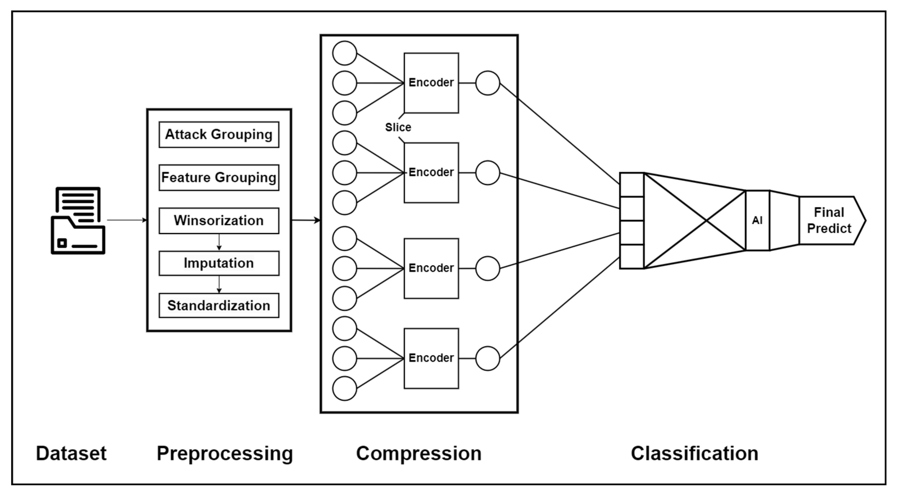
This section describes the experiments conducted to train and evaluate the proposed Autoencoder-SVM-based multi-class malicious traffic detection model. The same preprocessing pipeline (Winsorization, Imputation, Group-wise Standardization) and data split (Train 70%, Validation 15%, Test 15%) were applied, and reproducibility was ensured by fixing the random seed and class weights (class_weight = ‘balanced’). The model’s computational resource usage was measured in real-time using Resource Sampler and a timer, and each experiment was designed to be evaluated not only for accuracy but also for efficiency and reliability in a balanced manner.

For the classification stage, all experiments employed an SVM classifier and the complete parameter configuration is summarized in

Table 5. Using Parameter of SVM.

Parameter	Value
Kernel	RBF
C	1.0
gamma	scale
Class weight	Balanced (0:1.0, 1:1.0, 2:1.0, 3:1.0, 4:1.0)
Probability	True
Random state	41–45
Method	Isotonic
CV	3

. The same SVM settings were applied consistently across Experiment Set 1–4 to ensure a fair comparison. As shown in Table 5, the SVM was configured using an RBF kernel (C = 1.0, gamma = scale), balanced class weight, probability estimation enabled and isotonic calibration with 3-fold cross-validation, with the random state varied from 41 to 45 in accordance with the overall experimental protocol.

The entire experiment consists of a total of four sets (Set 1–4), each designed to analyze the performance and efficiency of the proposed model from different objectives and perspectives.

The first set of experiments (Set 1) for comparing SVM performance by autoencoder structure is conducted to analyze the impact of changes in autoencoder structure on the detection performance of the SVM classifier. This experimental setting compares the following four model configurations.

(1)

B1 (Raw + SVM): A base model trained by directly inputting the preprocessed original features.

(2)

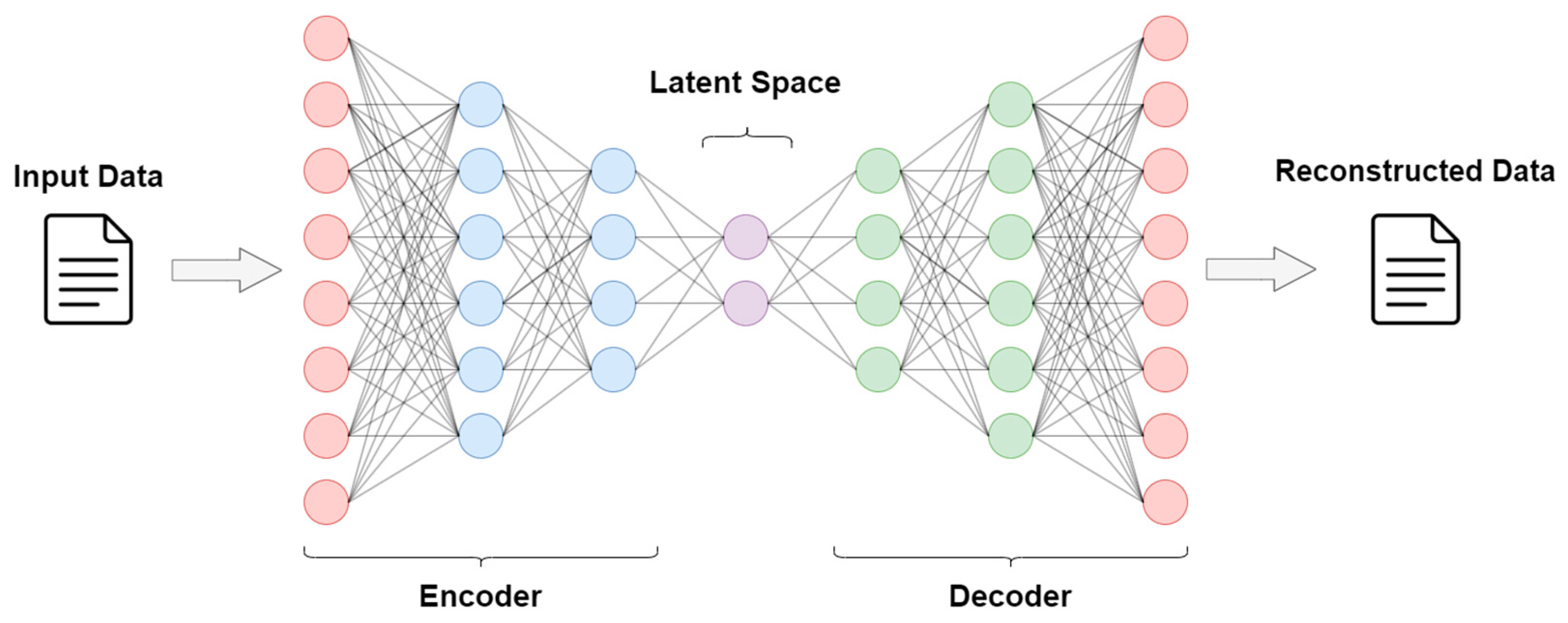
B2 (Single-AE + SVM): The latent representation obtained by compressing all features with a single autoencoder is used as input for the SVM. The encoder structure of the Single-AE model compresses 55 input features into a 13-dimensional latent representation for SVM classification, as shown in

Table 6. Autoencoder Architecture of B2 (Single-AE + SVM).

Stage	Layer (Type)	Output Shape	Param
Single-AE	InputLayer	(None, 55)	0
	Dense	(None, 27)	1512
	Latent	(None, 13)	364

.

(3)

B3 (Multi-AE + SVM): Independent autoencoders for each feature group (Volume, Size, Timing, Session, Subflow, and Active) separated by domain are trained, and then the latent representations from each group are merged to be used as input for the SVM. The encoder structure of the Multi-AE model independently encodes nine feature groups and concatenates them into a 28-dimensional latent vector, as shown in

Table 7. Autoencoder Architecture of B3 (Multi-AE + SVM).

Stage	Layer (Type)	Output Shape	Param
Multi-AE	InputLayer	(None, 9)	0
	Dense	(None, 16)	160
	Latent	(None, 4)	68

.

(4)

B4 (MultiSingle-AE + SVM): A structure that removes redundant representations and maximizes efficiency by further compressing the latent representation generated by the Multi-AE into a single autoencoder for secondary compression. The two-stage encoder structure of the Multi→Single-AE model further compresses the 28-dimensional multi-AE latent representation into 7 dimensions to improve efficiency, as shown in

Table 8. Autoencoder Architecture of B4 (MultiSingle-AE + SVM).

Stage	Layer (Type)	Output Shape	Param
Multi-AE	InputLayer	(None, 9)	0
	Dense	(None, 16	160
	Latent	(None, 4)	68
Single-AE	InputLayer	(None, 28)	0
	Dense	(None, 16)	464
	Latent	(None, 7)	119

.

Table 9. Compression Characteristics of Autoencoder based Models.

Model	Input Dim	Latent 1	Latent 2	Ratio	Reduction (%)
B1_raw_SVM	55	-	-	1.0000	0.00%
B2_single-AE_SVM	55	13	-	0.2364	76.36%
B3_multi-AE_SVM	55	28	-	0.5091	49.09%
B4_multiSingle-AE_SVM	55	28	7	0.1273	87.27%

provides a comparative summary of how each model compresses the original 55-dimensional input features. All models determine their latent dimensions using the same rule-based scheme, where the latent size is set to one-fourth of the input dimension (e.g., 55/4 ≈ 13) and constrained within a minimum of 4 and a maximum of 64 units. Following this rule, the single-AE model B2 produces a 13-dimensional latent vector. The multi-AE model B3 also applies the same compression rule but divides the input features into six groups, applies a separate 1/4-scaled encoder to each group, and then concatenates the six latent outputs. As a result, the final latent dimension becomes 28. Thus, both B2 and B3 follow an identical per-encoder compression principle, and the difference in latent size arises from architectural design rather than differences in compression policy. In contrast, B4 employs the most aggressive two-stage encoding process, ultimately reducing more than 87% of the original input dimension.

For each model, the training results and inference time were measured by separating the encoding and classification stages, and memory usage and throughput were also recorded. The main purpose of this experiment is to reveal the correlation between the structural complexity and performance of autoencoders and to determine a balance between computational efficiency and detection accuracy.

The second set of experiments (Set 2) for comparing resource usage and encoding efficiency analysis by model structure is conducted to quantitatively analyze the computational resource consumption characteristics of each model structure. For the four models (B1–B4) used in Set 1, the hardware resource utilization is measured separately for the encoding and classification stages. The metrics are measured based on a total of three criteria: CPU memory usage (RSS mean/max), GPU utilization (GPU utilization mean/max), and GPU memory usage (GPU VRAM mean/max). This experiment aims to analyze the impact of extending the autoencoder structure on system resource consumption and to evaluate the practical cost of increased structural complexity on computational efficiency.

The third set of experiments (Set 3) for comparing classifiers based on Multi-AE representation is conducted to compare the detection performance among various classifier models using the latent representation generated through the Multi-AE preprocessing step in the proposed B3 model as a fixed input. In this experiment, several machine learning-based classifiers, including SVM, are compared under the same input conditions. The models used are shown in

Table 10. Classifier Model.

Type of Classifier	Model
Kernel-based Models	Support Vector Machine (SVM)
Linear Models	Logistic Regression (LR)
Tree-based Models	Decision Tree (DT)
	Random Forest (RF)
	Extra Trees (ET)
	Gradient Boosting (GB)
	HistGradientBoosting(HGB)
Instance-based Models	K-Nearest Neighbors (KNN)
Neural Network-based Models	Multi-layer Perception (MLP)
Boosting-based Ensemble Models	XGBoost (XGB)
	LightGBM (LGBM)
	CatBoost (CatBoost)

. This experiment aims to show that the proposed autoencoder-based latent representation is not dependent on a specific classifier structure and exhibits consistent detection performance across various learning algorithms.

The fourth set of experiments (Set 4) is conducted to verify whether the proposed model can meet Service Level Agreement (SLA) constraints in a 5G slicing environment. Measurements on an actual 5G network are not performed, but instead our inference results are compared by setting the SLA limit values from public literature as a reference. For the finally selected model (SVM-based Multi-AE structure), the mean/95% latency and throughput are measured while varying the inference batch size to 1, 8, 32, 128, and 512. Additionally, per-class latency is calculated to analyze real-time detection deviations based on attack types. The SLA baseline is as a reference, and whether the model meets the ultra-low latency and high throughput requirements is verified. This experiment aims to verify the inference efficiency and real-time responsiveness of the proposed model and to derive the optimal processing configuration based on batch size.

These four sets of experiments were designed to evaluate performance comparisons based on the structural differences in the autoencoder, the efficiency of computational resource consumption, the generalization performance related to latent representation, and the possibility of real-time detection under SLA constraints. Through this phased experimental design, the proposed model is structured to enable a comprehensive performance analysis that goes beyond simple accuracy evaluation, considering efficiency, reliability, and real-time performance in an actual 5G slicing environment.

5.4. Experimental Results

5.4.1. (Set 1) Comparison of SVM Performance by Autoencoder Structure

The detailed detection characteristics of each model were analyzed through the class-wise F1-score results in

Table 11. Average Metric by Model & Label over random states 41–45.

Label	Metric	B1_Raw_SVM	B2_Single-AE_SVM	B3_Multi-AE_SVM	B4_Multisingle-AE_SVM
Benign	Precision	1.0000	0.9997	0.9996	0.9999
	Recall	0.9993	0.9991	0.9991	0.9909
	F1-Score	0.9997	0.9993	0.9996	0.9954
San Attack	Precision	0.9993	0.9991	0.9995	0.9887
	Recall	0.7582	0.7623	0.7591	0.7579
	F1-Score	0.8599	0.8652	0.8648	0.8580
TCP PUSH	Precision	0.9818	0.9682	0.9788	0.7394
	Recall	1.0000	0.7231	0.9077	0.7024
	F1-Score	0.9908	0.8686	0.9868	0.6665
TCP SYN	Precision	1.0000	1.0000	0.9997	0.9997
	Recall	1.0000	1.0000	1.0000	1.0000
	F1-Score	1.0000	1.0000	1.0000	0.9998
TCP URG	Precision	0.8023	0.6812	0.7562	0.6534
	Recall	0.9814	0.9886	0.9783	0.7269
	F1-Score	0.8828	0.8274	0.8738	0.7163

. which represent the average values calculated over random states 41–45 for generalized performance evaluation. In the case of Benign, the F1-score remained above 0.99 for all models, showing very high stability. This data indicates that normal traffic has a structurally consistent pattern and is relatively less sensitive to changes in the autoencoder structure. For the Scan Attack class, all models showed consistently high precision in the range of 0.99–0.98, while recall remained around 0.76 across the board. Within this narrow performance band, the B3 model achieved a balanced score with a precision of 0.99, recall of 0.76, and F1-score of 0.86, demonstrating the most stable and consistent behavior among the models. Although scan traffic is structurally simple B3 maintains robustness by preserving essential features without excessive compression, resulting in highly reliable detection.

The TCP PUSH class exhibited the largest performance variation across models, and this is where the advantages of the B3 structure became most evident. B3 achieved a precision of 0.98, recall of 0.91, and an F1-score of 0.98, nearly matching the best performance of B1 while significantly outperforming both B2 and B4. In contrast, B2 dropped to an F1-score of 0.87 due to a sharp decrease in recall, and B4 degraded drastically to 0.67 because of aggressive two-stage compression. These results highlight B3’s ability to reduce dimensionality effectively while retaining fine-grained attack-specific patterns, making it the most balanced model between compression and detection accuracy.

For the TCP SYN class, all models consistently maintained excellent detection performance, since SYN flood attacks exhibit a highly repetitive and predictable connection-request pattern. As a result, the autoencoder structure has minimal influence on the classifier’s ability to distinguish this traffic type.

The TCP URG class showed the greatest instability overall, with precision varying from 0.65 to 0.80 and recall from 0.73 to 0.98 across models. Despite this variability, B3 produced the most effective and stable results, achieving a precision of 0.75, recall of 0.98, and an F1-score of 0.87, outperforming the other models. B4 dropped significantly to 0.71, and B2 achieved 0.82, showing inconsistent behavior. B3’s multi-AE architecture effectively captures the irregularity and low session consistency of URG traffic without introducing excessive compression, enabling superior detection stability.

As shown in

Table 12. Evaluation Metric by Model.

Model	Accuracy	Macro f1	Balanced Accuracy	ECE
B1_raw_SVM	0.9478	0.9471	0.9477	0.0422
B2_single-AE_SVM	0.9104	0.9107	0.9104	0.0308
B3_multi-AE_SVM	0.9285	0.9283	0.9285	0.0320
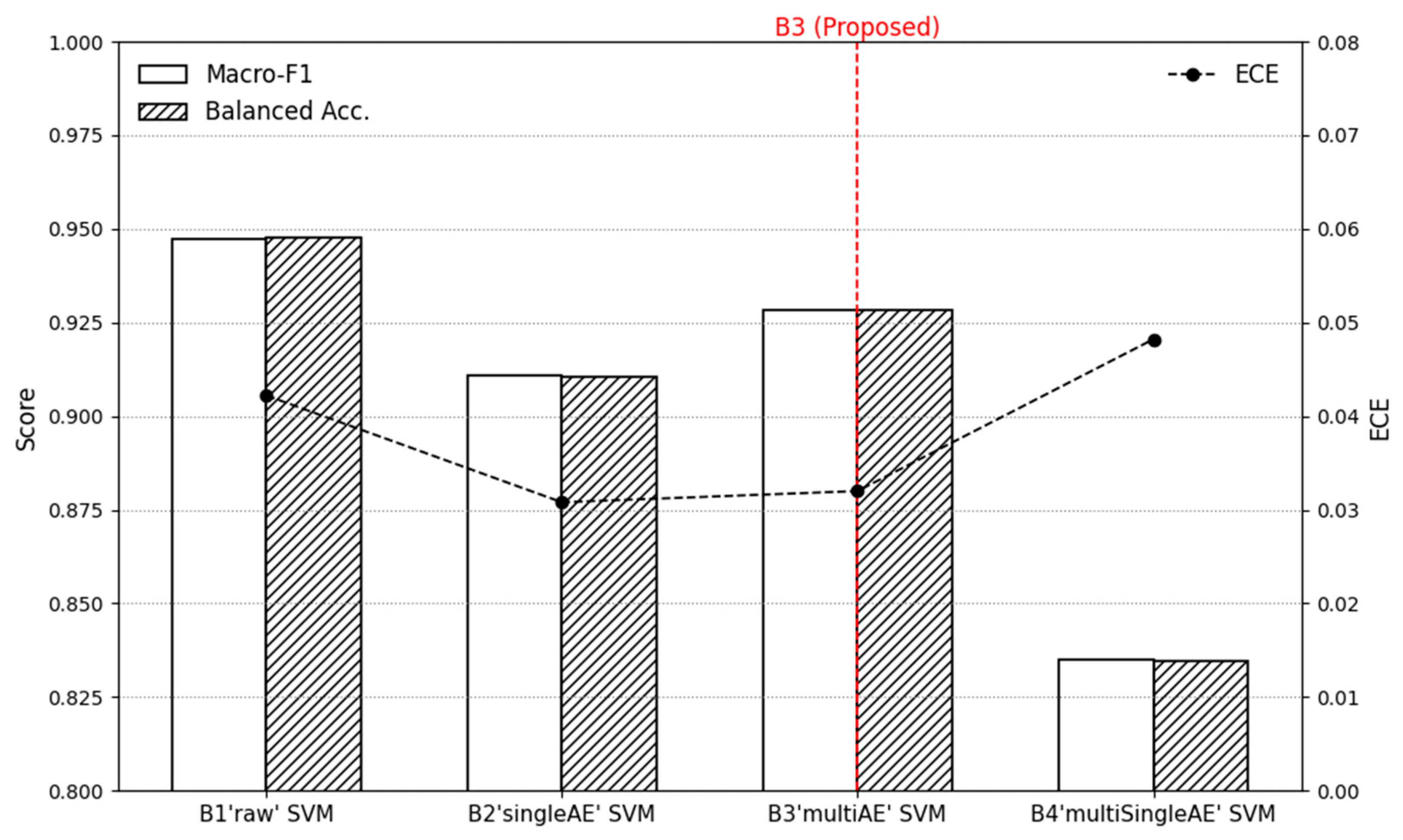
B4_multiSingle-AE_SVM	0.8345	0.8351	0.8345	0.0482

and Figure 3, the performance differences across autoencoder structures become clear when evaluated under identical conditions. The B1 model, which uses raw features without any compression, achieved the highest scores overall, recording an accuracy of 0.95 and a macro F1-score of 0.95. This strong performance is expected, as the model directly leverages the full 55-dimensional feature space without any loss of information. The B2 model, which applies to a single autoencoder with a latent size of 13, showed a slight performance decrease compared to B1, with accuracy and macro F1 both around 0.91. This indicates that a single AE tends to capture only global patterns and is less effective in expressing class-specific feature variations. The B3 model, using the Multi-AE structure with six group-wise encoders and a concatenated latent dimension of 28, achieved moderately improved generalization compared to B2, showing consistent values across accuracy (0.93), macro F1 (0.93), and balanced accuracy (0.93). Its ECE score (0.03) also remained low, suggesting that the model’s probability estimates are more reliable. This improvement can be attributed to the Multi-AE structure independently learning each group’s characteristics, allowing the latent representation to capture finer inter-class distinctions without deviating from the unified com-pression rule. The B4 model, which performs the most aggressive two-stage compression, showed the largest performance drop, with accuracy and macro F1 decreasing to approximately 0.83. This result is consistent with the fact that B4 reduces more than 87% of the feature space, causing loss of detailed information that would otherwise assist in separating similar classes.

5.4.2. (Set 2) Comparison of Resource Usage and Encoding Efficiency Analysis by Model Structure

Table 13. Memory Usage (RSS) by Model.

Model	Encoding 1 (MB, Mean/Max)	Encoding 2 (MB, Mean/Max)	Evaluation (MB, Mean/Max)
B1_raw_SVM	-	-	6100.2/6100.4
B2_single-AE_SVM	5734.6/6100.4	-	5948.8/5957.3
B3_multi-AE_SVM	5630.5/5957.4	-	5869.4/5883.2
B4_multiSingle-AE_SVM	3166.7/3180.4	3166.7/3180.4	3166.7/3180.4

,

Table 14. GPU Utilization (%) by Model.

Model	Encoding 1 (Mean/Max)	Encoding 2 (Mean/Max)	Evaluation (Mean/Max)
B1_raw_SVM	0.0/0.0	-	0.0/0.0
B2_single-AE_SVM	1.4/5.0	-	0.0/0.5
B3_multi-AE_SVM	1.0/7.0	-	0.0/0.0
B4_multiSingle-AE_SVM	0.0/0.5	0.0/0.5	0.0/0.5

and

Table 15. GPU Memory Usage (MB) by Model.

Model	Encoding 1 (Mean/Max)	Encoding 2 (Mean/Max)	Evaluation (Mean/Max)
B1_raw_SVM	-	-	390.0/390.0
B2_single-AE_SVM	390.0/390.0	-	390.0/390.0
B3_multi-AE_SVM	390.8/391.0	-	391.0/391.0
B4_multiSingle-AE_SVM	387.0/387.0	387.0/387.0	387.0/387.0

show the results for memory usage, utilization, and GPU memory occupancy of the proposed model (B3) and the comparison models.

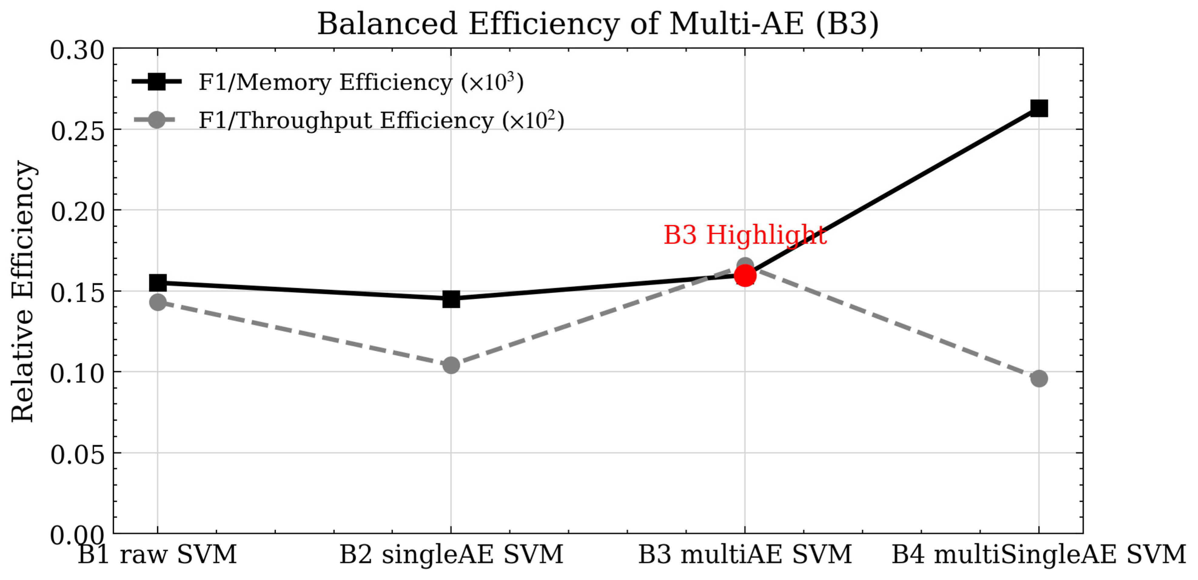
Table 13 shows that the B1 model had the highest memory usage at approximately 6.1 GB, and the B2 model, which uses a single autoencoder, was also at a similar level of 5.9 GB, with no significant difference. On the other hand, the proposed model, B3, efficiently used memory with an average of 5.7 GB, despite employing a parallel encoder structure. This is interpreted as being because each feature group undergoes an independent encoding process, minimizing unnecessary parameter redundancy. Finally, B4 showed the lowest usage at 3.1 GB, but in the previous evaluation, it was confirmed that excessive compression resulted in loss of information, leading to a significant drop in detection rate. In 5G network slicing environments, such differences in memory usage are directly linked to slice-level resource availability and service isolation. Excessive memory consumption in one slice can reduce the available resources for other slices and may lead to degraded SLA performance.

In the GPU utilization analysis results of Table 14, the GPU occupancy of all models was measured to be less than 10%, confirming stable operation is possible even in a real-time 5G traffic analysis environment. Specifically, the B3 model showed a maximum GPU utilization of 7% during the Learning Encoding 1 process, which was confirmed to be a temporary load due to parallel encoding operations. In terms of GPU efficiency, it is still confirmed to be a lightweight structure. Such low GPU load is crucial in slicing-based deployments, since shared GPU resources across slices are highly sensitive to temporary spikes. Excessive utilization may introduce scheduling delays and jitters, especially in URLLC-focused slices.

The GPU memory usage results in Table 15 show that there was little difference between the models, and all models remained stable at around 390 MB. In MEC or slice environments where GPU memory is limited maintaining a small and stable memory footprint helps prevent resource contention and contribute to predictable real-time behavior.

Figure 4 visually represents the results in the table, showing that the proposed model (B3) achieved the best balance between detection performance and resource usage. B3 achieved approximately 5% less memory usage than B1 while maintaining the same level of detection accuracy. It also gained the advantage of improved performance and reduced resource usage compared to B2. This balance is particularly important in slicing environments where resource overload in one analytic component can negatively impact other coexisting slices.

In summary, the B3 model based on Multi-AE has been proven to be a lightweight structure that minimizes hardware resource consumption while achieving improved information representation and generalization performance compared to a single AE.

5.4.3. (Set 3) Comparison of Classifiers Based on Multi-AE Representation

Set 3 compared the detection performance across various classifiers to verify the generalization performance of the proposed Multi-AE-based latent representation. This experiment analyzed performance differences based on classifier structures by using the features encoded through Multi-AE (latent features) as fixed inputs. All models applied the class_weight = “balanced” option to correct for class imbalance and performed isotonic calibration-based calibration to improve the reliability of predicted probabilities.

Table 16. Matric by Multi-Classifier.

Classifier	Accuracy	Macro F1	Balanced Accuracy	ECE	Mean RSS(MB)
LR_balanced	0.9319	0.9324	0.9319	0.1026	6119.7
DT_balanced	0.9598	0.9597	0.9598	0.0029	5766.6
RF_balanced	0.9595	0.9594	0.9595	0.0028	5847.2
ET_balanced	0.9598	0.9597	0.9598	0.0028	5895.9
HGB	0.9602	0.9600	0.9602	0.0029	5925.8
GB	0.9606	0.9604	0.9606	0.0040	5926.2
KNN	0.9589	0.9587	0.9589	0.0045	5930.4
MLP	0.9497	0.9488	0.9496	0.0150	5931.5
XGB	0.9601	0.9599	0.9601	0.0030	5955.3
LGBM	0.9601	0.9599	0.9601	0.0028	5986.5
CatBoost	0.9601	0.9599	0.9601	0.0034	6279.8
SVM	0.9406	0.9398	0.9406	0.0272	5869.4

shows the results of comparing the performance (accuracy, macro F1, balanced accuracy), prediction confidence (ECE), and resource efficiency (mean RSS) of each classifier. Most classifiers achieved accuracy above 0.95, confirming that the Multi-AE latent feature provides consistent detection performance across different models. Specifically, ensemble-based models (GB, HGB, XGB, LGBM) showed high detection performance around 0.96 and very low ECE (0.0028–0.0040), demonstrating that Multi-AE provides stable feature representation capabilities. On the other hand, the model using the proposed SVM model showed slightly lower values, but its resource efficiency was excellent compared to its model complexity. The mean RSS is around 5.8 GB, maintaining a lower memory footprint than most boosting models. In short, the Multi-AE-based feature representation method maintained consistent detection performance without being dependent on the classifier structure, and the proposed model achieved the best balance between performance and resources.

5.4.4. (Set 4) Comparison of SLA Constraints Met by Model

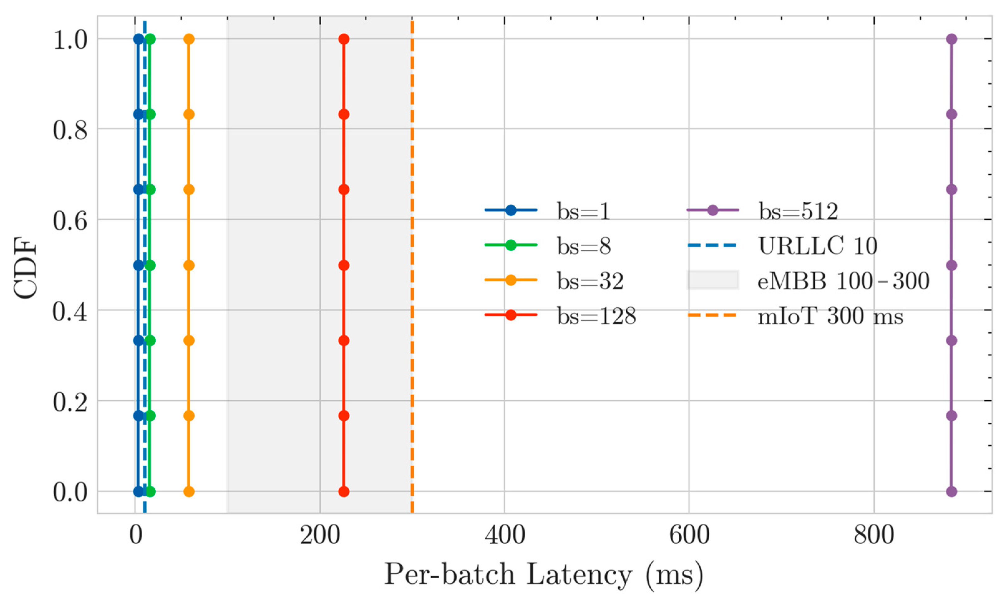
Figure 5 shows that the latency distributions for all batch sizes fall within the SLA region. Specifically, in the bs ≤ 128 range, there is a low latency distribution that meets the 10 ms URLLC criteria. This means that the proposed Multi-AE encoding generated a lightweight latent representation, thereby reducing inference time.

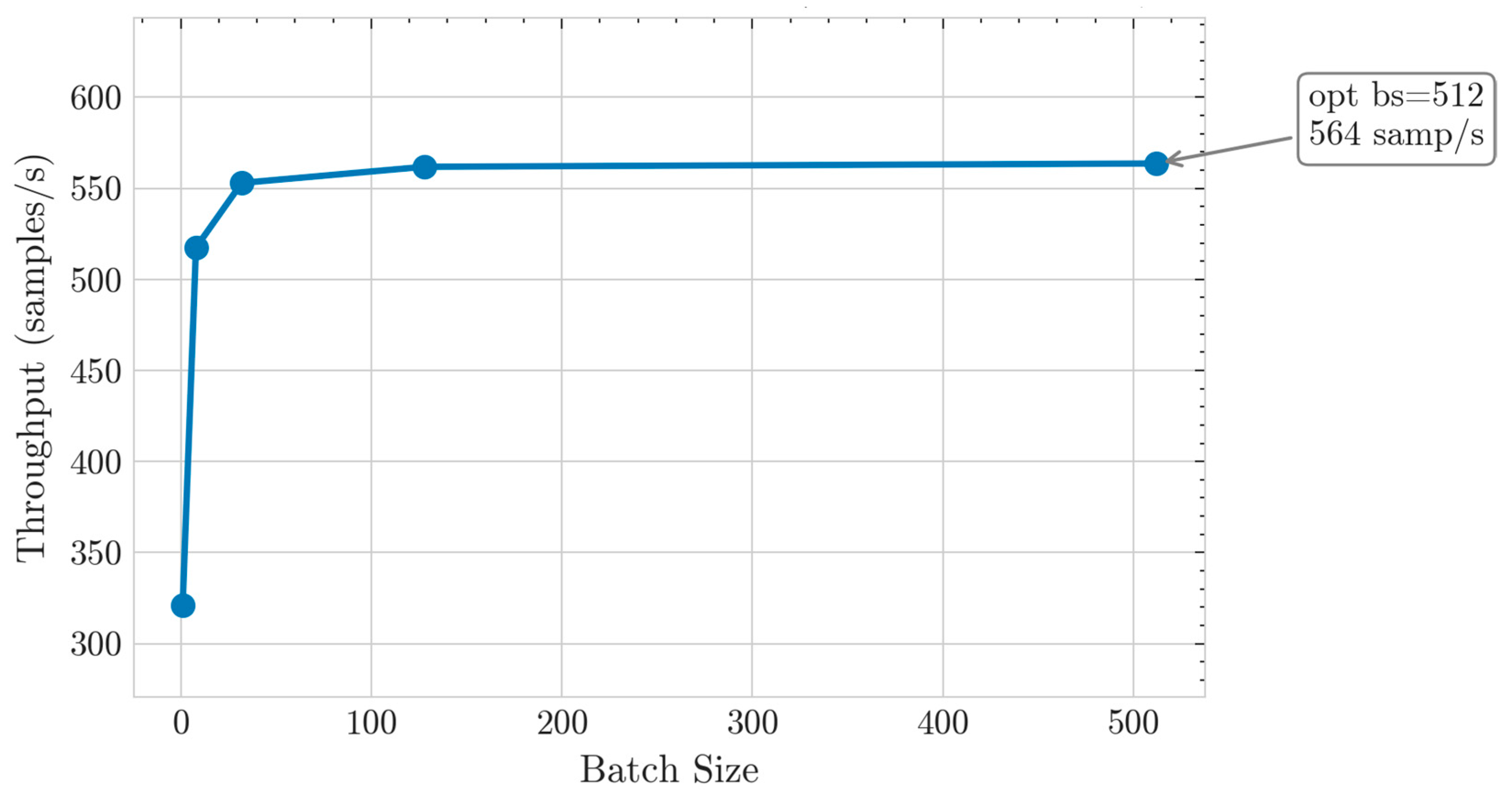
The throughput curve in Figure 6 increases exponentially in the bs (batch size) = 1–8 range, saturates from bs ≥ 128, and achieves a maximum throughput of 564 samples/s at the optimal batch size (bs = 512). This indicates the point where the balance between inference efficiency and latency is optimal, making it a suitable operating point for real-time eMBB services or industrial sensor network environments.

6. Discussion and Conclusions

This study proposed an autoencoder-based multi-class malicious traffic detection framework that satisfies real-time performance, lightweight design, and accuracy in a private 5G network slicing environment. The proposed model achieved high accuracy and resource efficiency even in complex 5G traffic structures by simultaneously considering slice-specific data characteristics and domain-specific traffic features.

The main implications of the experimental results are as follows. First, the Multi-AE structure effectively reflected inter-class variability and slice characteristics compared to a single autoencoder and maintained high detection performance (accuracy 0.93, balanced accuracy 0.93) even with complex traffic patterns. This is the result of the group-wise autoencoders independently learning the correlations between features, minimizing loss of information. Second, the SVM-based lightweight classifier-maintained GPU utilization below 7% and memory usage around 5.7 GB, demonstrating its potential for real-time application. Third, the SLA verification results demonstrated that inference latency of 10 ms or less and throughput of 564 samples/s were achieved based on URLLC standards, proving stable detection is possible even in eMBB and industrial mIoT environments. This is not simply an accuracy-focused model but an approach that considers the practical operational conditions of 5G slicing.

The results of this study differ from previous research in several aspects. Prior autoencoder-based IDS studies mainly focused on global feature learning in single network settings, whereas this work integrates slice-aware preprocessing and group-based encoding to incorporate both the structural properties and SLA requirements of 5G slicing. This enables behavior-aware and slice-level classification beyond simple anomaly detection and achieves efficient resource utilization suitable for real time response. However, the dataset used in this study has a limited slice configuration derived from an experimental environment. Future research will expand the number and types of slices, conduct generalization tests on large, heterogeneous datasets, and evaluate detection robustness in a wider variety of slicing environments.

Beyond experimental validation, a deep understanding of how the proposed model can be operationally deployed and managed in a real-world 5G slicing environment is essential. To achieve this, we present a three-phase deployment roadmap. First, we conduct simulation-based end-to-end evaluations to quantify the inference latency introduced by the model, analyze processing bottlenecks, and ensure that the total latency remains within URLLC-level performance limits. Second, we perform testbed-level validation using Open5GS or a comparable 5G core system. This allows us to integrate the model into the control-plane and user-plane workflows through standardized interfaces such as REST APIs or gRPC telemetry, enabling the measurement of real-world inference latency, queuing delay, and interactions with Network Functions (e.g., AMF, UPF).

The final phase involves integrating the proposed model into a production scale 5G slicing environment through compatibility with ETSI NFV-MANO, SDN controllers, and NWDAF-based analytics frameworks. This includes slice-level validation, multi-slice stress testing, and scalable deployment across distributed MEC nodes. As part of this roadmap, the model’s inference latency will be benchmarked across the entire end-to-end processing chain including data collection, preprocessing, encoding, classification, and alert forwarding to accurately assess the operational delay introduced by the detection engine.

Furthermore, future research will evaluate the model under high-load traffic scenarios to analyze how resource efficiency and real-time behavior change under slice congestion or bursty traffic conditions. This analysis will provide in-depth insights into the model’s operational robustness and scalability in realistic 5G environments where dynamic load fluctuations frequently occur.

In conclusion, the proposed Multi-AE-based multi-class classification framework demonstrates improved accuracy, lightweight computation, and operational stability, satisfying the Service Level Agreement (SLA) requirements that are essential for 5G slicing environments. By combining group-based autoencoders with a Support Vector Machine (SVM) classifier, the model efficiently distinguishes multiple attack types while maintaining low latency and high throughput. This study provides a practical foundation for automated security and intelligent threat detection in private 5G networks. Future work will validate the model’s real-time performance using a full 5G testbed.