Article

Optimizing Vehicle Emission Estimation of On-Road Vehicles Using Deep Learning Frameworks

1
Department of Electrical Electronic Engineering, Zonguldak Bulent Ecevit Üniversity, Zonguldak 67100, Türkiye
2
Department of Geomatics Engineering, Zonguldak Bulent Ecevit Üniversity, Zonguldak 67100, Türkiye
*
Author to whom correspondence should be addressed.
Appl. Sci. 2025, 15(22), 12235; https://doi.org/10.3390/app152212235
Submission received: 17 October 2025 / Revised: 6 November 2025 / Accepted: 10 November 2025 / Published: 18 November 2025

Abstract

Vehicle, industrial, and urban emissions remain major contributors to air quality degradation, affecting public health and the level of environmental cleanliness. Cost-effective specific pollutant estimation models, i.e., for carbon monoxide  CO , carbon dioxide  CO 2 , and ammonia  NH 3 , are essential to tackle the practical challenge of high-resolution monitoring for reducing vehicle emissions in traffic. Existing model design methods, however, may be insufficient, particularly for peak time estimations, since such models are typically designed using gridding-based vehicle-specific power polynomial and non-optimized artificial neural networks. In this paper, we propose vehicle emission models of pollutants based on a Bayesian Monte Carlo (MC) Dropout-based robust data-driven gated recurrent unit (BMC-GRU) method to enhance estimation robustness and mitigate the overfitting problem in the deep learning network. Bayesian optimization determines the optimal architecture by efficiently and probabilistically searching the hyperparameters of the network, while MC-Dropout quantifies epistemic uncertainty through multiple stochastic forward passes during testing. Therefore, the proposed method improves the models’ calibrations and robustness to distribution shifts. For benchmarking, least squares-based first- and fourth-order polynomials, conventional long-short term memory (LSTM), and bidirectional LSTM (BiLSTM)-based estimation models are designed. The proposed method outperforms the mentioned state-of-the-art methods with strong robust estimation performance. The experimental results on multiple real-world vehicle datasets demonstrate that the proposed method significantly outperforms state-of-the-art approaches. The method presents a promising solution for uncertainty-aware vehicle emission modeling that is applicable to transportation systems.

1. Introduction

The air quality of the environment remains a major concern since urbanization, industrial factories, and gasoline/diesel engine-powered vehicles increase air pollution [1,2,3,4]. The United States Environmental Protection Agency (US-EPA) declared that several major pollutants, i.e., carbon monoxide ( CO ), carbon dioxide ( CO 2 ), and ammonia ( NH 3 ), pose a significant risk, where such pollutants are monitored in vehicle exhaust gas [5,6]. Some researchers have found that vehicle emissions have considerable impacts on the air quality of the environment, particularly under heavy traffic conditions [7]. The remote on-board diagnostic (OBD) system, which can perform wireless data transmission, can measure vehicle parameter identities (IDs) in real time, which can be a key component in characterizing the air gas pollutants of vehicles [8]. Such vehicle parameter IDs include instantaneous engine revolution, fuel consumption, velocity, temperature, and acceleration vs. the vehicle and transmission. The system can send on- and off-road parameter IDs to a user device in a wireless environment [9,10]. The key factors affecting the fuel consumption and emission rate of vehicles are summarized in [11]. Some researchers have shown that performing real-time estimation of vehicles is challenging, although vehicle parameters can be measured [12,13].
The United States Environmental Protection Agency used a motor vehicle emission simulator (MOVES) and MOBILE model to estimate emissions from diesel and gasoline-powered vehicles [14,15]. The estimation accuracy of the models may be insufficient since the models present different estimation rates between  10 %  and  45 %  under some road conditions [16,17]. Therefore, simple linear regression equations are derived to estimate vehicle emissions using the MOBILE model based on vehicle model year, average vehicle speed, and air temperature, where the equation varies according to vehicle type [18]. The real-time vehicle emission and fuel consumption of vehicles are conventionally estimated based on vehicle-specific power (VSP) [19,20]. This method requires multiple specific parameters of a vehicle and air, i.e., vehicle mass, the translational mass of the rotating components, road grade, coefficient of rolling resistance, ambient air density, headwind into the vehicle, etc., which makes the estimation specific to the vehicle [21]. A one-dimensional polynomial is derived to estimate the instantaneous power demand of the vehicle using only the vehicle’s specific parameters [22]. Another one-dimensional polynomial is constructed to characterize energy consumption rates based on on-road data in Lisbon, Portugal, for motorcycles [23]. However, VSP-based methods evaluate vehicle emission based on discrete vehicle velocity, which reduces the prediction accuracy of actual emissions under on- and off-road conditions. The method also assumes that instantaneous high gas emissions due to vehicle stopping and starting caused by traffic conditions on rough terrain are a constant value. The machine learning method, i.e., AdaBoost, random forest, and support vector machine, is proposed to estimate the emissions within and outside the vehicle [24,25,26,27,28]. High-frequency components and high-emission/intensity peaks of the actual emission data could not be estimated, where training/validation often occurs with random or short-horizon time. Artificial neural networks (ANNs) and deep learning techniques can provide sufficient and necessary solutions to the problems of developing estimation models thanks to the exponential increase in data collection opportunities in the big data era. An ANN virtual sensor-based method was proposed to predict vehicle emissions in a laboratory environment by neglecting real-world traffic conditions [29]. An estimation model was proposed using an ANN based on data mining and GIS models on the New Klang Valley Expressway, Malaysia [30]. However, the hyperparameters of these networks are tuned using manual search, which is time-consuming [31,32,33]. A genetic algorithm-assisted ANN method was proposed to optimize the hyperparameters of the network to obtain sufficient estimation performance [34,35]. The performance of this model, however, is based on the defined range of the hyperparameters and presents non-unique solutions because of the non-convex nature of the algorithm. Long short-term memory (LSTM) network-based methods have been proposed for vehicle emission pollution prediction using PEMS and OBD systems [36,37,38]. However, these methods present uncertainties and the overfitting problem during the training process. The selection of hyperparameters of the network is based on manual search and prior knowledge of the designer. A hyperparameter tuning approach is proposed using the particle swarm algorithm for an LSTM-based model [39]. Gated recurrent unit (GRU)-based estimation models present a promising solution since the network can achieve better estimation accuracy with limited data [40,41]. The hybrid genetic algorithm-GRU method was proposed to optimize the hyperparameters of the network [42], and it does not interfere with the deep learning process. However, the uncertainties and overfitting problems of the network still remain, which may necessitate rerunning the algorithm multiple times to obtain a performance-optimized model.
In order to contribute to filling in the mentioned research gap, we propose an automatically tuned data-driven robust Bayesian Monte Carlo gated recurrent unit (BMC-GRU)-based vehicle emission estimation model for gasoline and diesel engine motor-based vehicles, where the hyperparameters of the network are optimized via Bayesian optimization. To decrease the network uncertainties and overfitting problems of the deep learning network-based system, we include the Monte Carlo Dropout approach in the training process of the estimation models. A high-quality dataset of vehicle parameters is obtained in various driving scenarios on rough country roads, stopped traffic, and free-flow roads to analyze the effects of these scenarios on the vehicle emission rate. The proposed method is compared with advanced AI-dependent state-of-the-art methods, i.e., LSTM and Bidirectional LSTM-network (BiLSTM)-based models, and ridge regression based on one-dimensional first- and fourth-order polynomials. The contributions of this study are as follows:
  • We propose a Bayesian GRU-network-based estimation method to optimize probabilistically the hyperparameters of the network, i.e., learning rate, batch size, number of hidden layers, and number of nodes in each hidden layer.
  • The method uses an uncertainty-aware emission estimation model that uses MC-Dropout to quantify epistemic uncertainty and Bayesian optimization to probabilistically tune hyperparameters, resulting in calibrated predictions and dependability against distribution drift.
  • The estimation model can achieve high-resolution performance accuracy using the velocity, revolutions per minute (RPM), throttle position, and mass air flow (MAF) sensor data of the vehicle from the OBD system. The dataset is collected under real road conditions, i.e., rough country roads, stopped traffic, and free-flow roads, using multiple vehicles.
The remainder of this paper is structured as follows: Section 2 presents the rich data collection process of the method using the two different vehicles. Section 3 introduces the Bayesian optimization, MC-Dropout approach, GRU, and LSTM networks. Section 4 presents the performance of the data-driven vehicle emission model results using statistical metrics. Section 5 concludes the paper.

2. System Description and Problem Formulation

The real-time vehicle-specific pollutant measurement system is presented in Figure 1, where the system is integrated on two gasoline engine-powered vehicles: a 2018 Opel Astra edition plus and a 2014 Nissan Juke. The Astra 1.6 (115 PS, 155 Nm) and the Juke 1.6 NA (113–117 PS, 144–158 Nm) share the same torque band; both have limited traction at low-to-mid revs and deliver power at high revs. These vehicles, which have similar engine displacement, power output, and fuel type (1.6 L, gasoline), were chosen to observe the impact of components other than engine type on the learning process. This way, the effects of variables such as mass, body form factor, and transmission/gear ratios, which affect pollutant emissions, are included in the learning process. The vehicles, therefore, offer comparability with their front-wheel-drive counterparts, similar power ratings, and common usage characteristics in the same market (urban/extra-urban). These similarities are further standardized by driving cycle, fuel type, tire grade, and regular maintenance requirements.
The throttle position, speed, MAF, and engine RPM data of the vehicles are obtained via the OBD-II interface, which presents the state information of the vehicles under all driving conditions. The MQ-7 sensor is used for  CO  measurement, which has a detection range between  [ 20 ,   2000 ]  parts per million ( ppm ); the MG-811 sensor is used for  CO 2  measurement, which has a detection range between  [ 400 ,   10,000 ] ppm ; and the MQ-137 sensor is used for  NH 3  measurement, which has a detection range between  [ 5 ,   500 ] ppm . These pollutant-specific sensors are placed near the tailpipe mouth at a position close to the exhaust outlet (out of direct contact with the hot stream and minimizing outside air entrainment) and were calibrated before each data collection in a three-step procedure: (i) controlling sensor outputs according to room conditions, (ii) manufacturing multi-point references, and (iii) verification of monotonic response to known ramp steps from their datasheet. The measured outputs of the sensors are verified prior to starting the vehicles on each route to avoid undesired environmental conditions on the measurement: sensor overheating and displacement at measurement points. Following the datasheet recommendations, the MQ-7 sensor is calibrated using a 10k load resistance value for 200 ppm CO in clean air [43]. The position of the vehicle is obtained using the NEO-6M global positioning system (GPS) sensor. Analog output voltages of all sensors are recorded and converted to concentration with the sensor-specific conversion rates. The data is obtained using an Arduino microprocessor.

Data Collection

A dataset is collected as a time series with a 10 Hz sampling frequency to obtain high-resolution deep learning-based specific pollutant estimation models. The vehicle’s inherent data, which is captured via the OBD-II interface, is connected to the Arduino CAN-BUS shield and is read through the connection of an Arduino Uno board integrated with the Arduino CAN-BUS shield. The algorithm for parsing the OBD-II data frame runs on the Arduino board. The vehicle, GPS, and sensors’ data is sent to the host computer using the serial communication interface at a baud rate of 9600–230,400 bit/s for processing in the Python environment. The dataset is filtered using a vector-based zero-phase filtering method to predict the model using the Python Keras 1.4.7 and TensorFlow 2.13.0 Libraries. The deep learning methods are trained on a host computer that has an Intel Core i7-10750H CPU, 2.6 GHz, and 32 GB RAM.
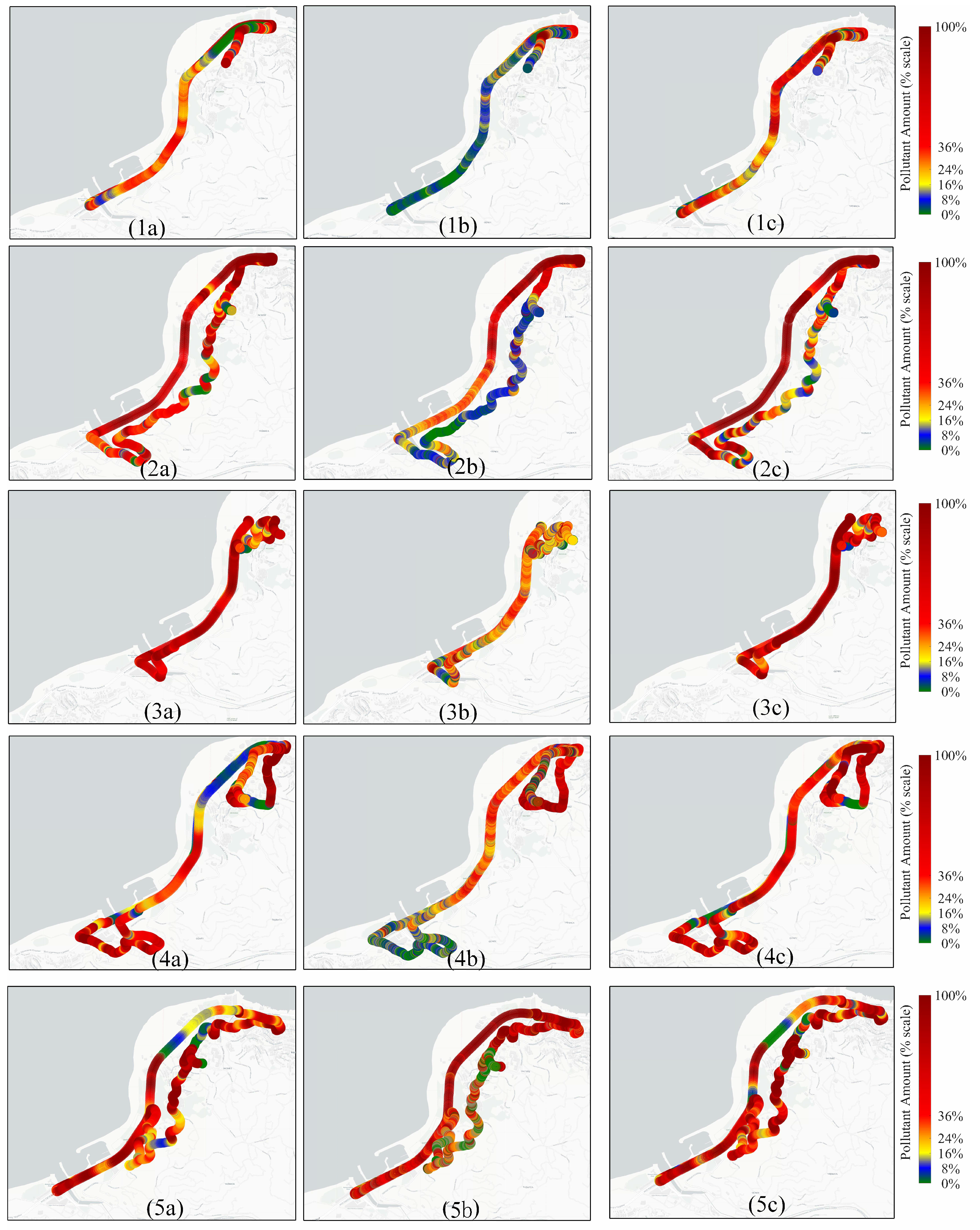
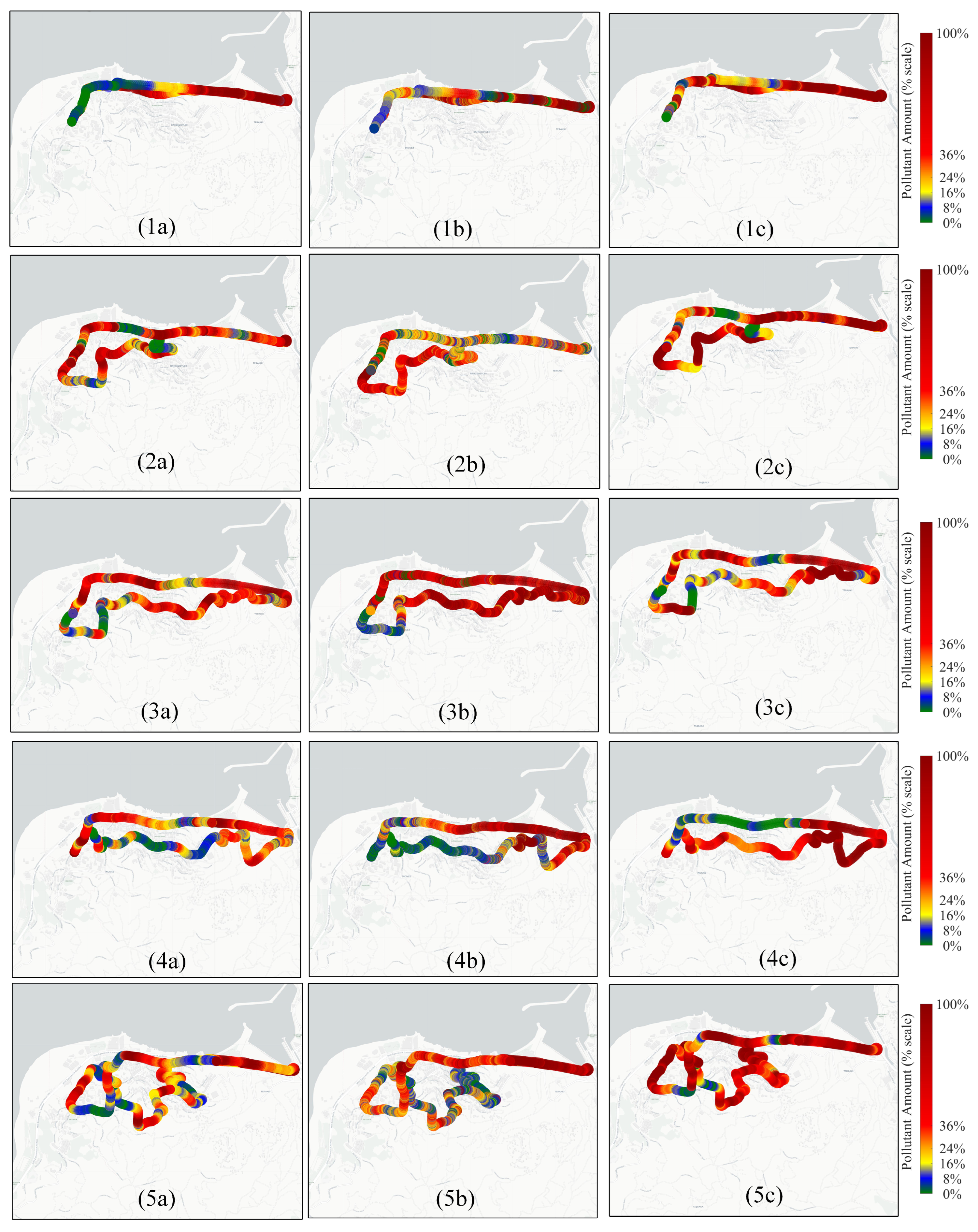
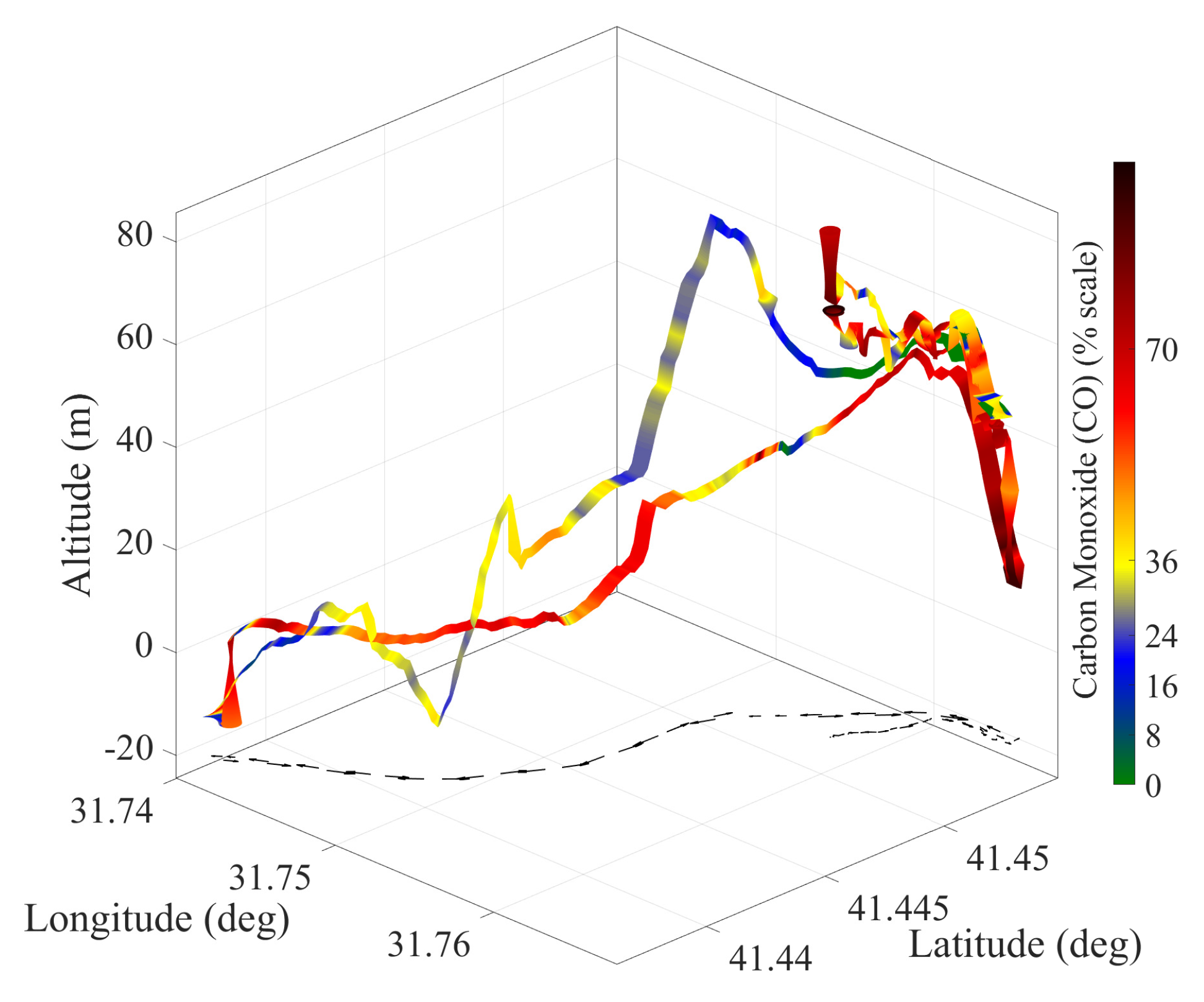
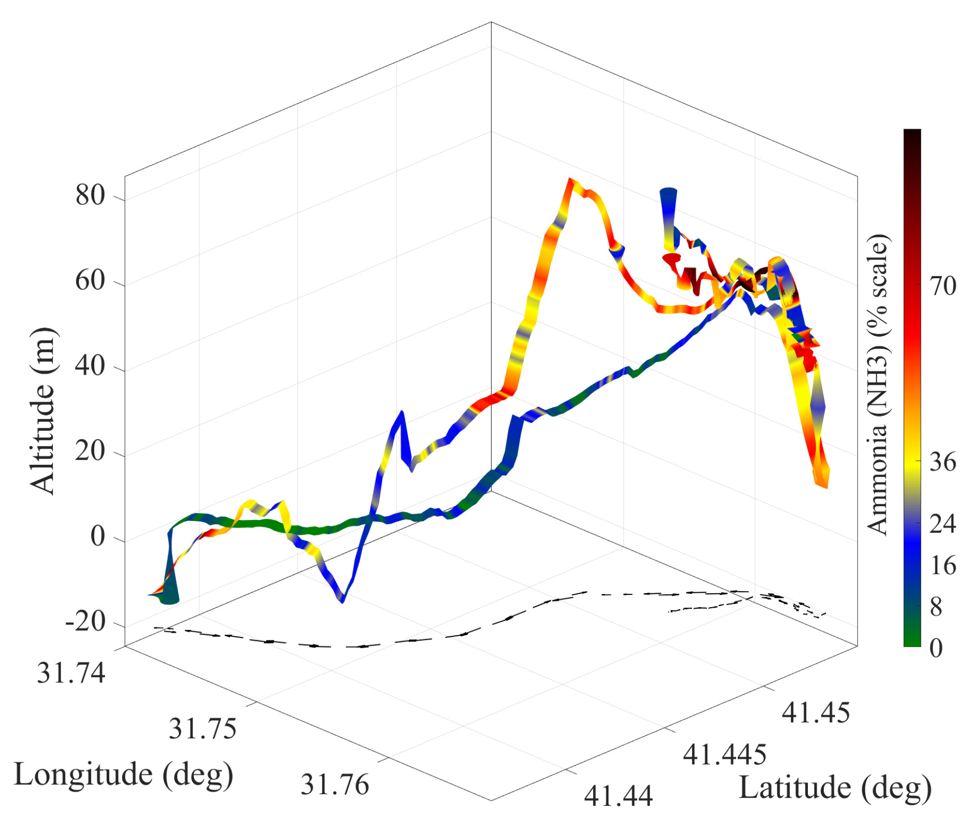
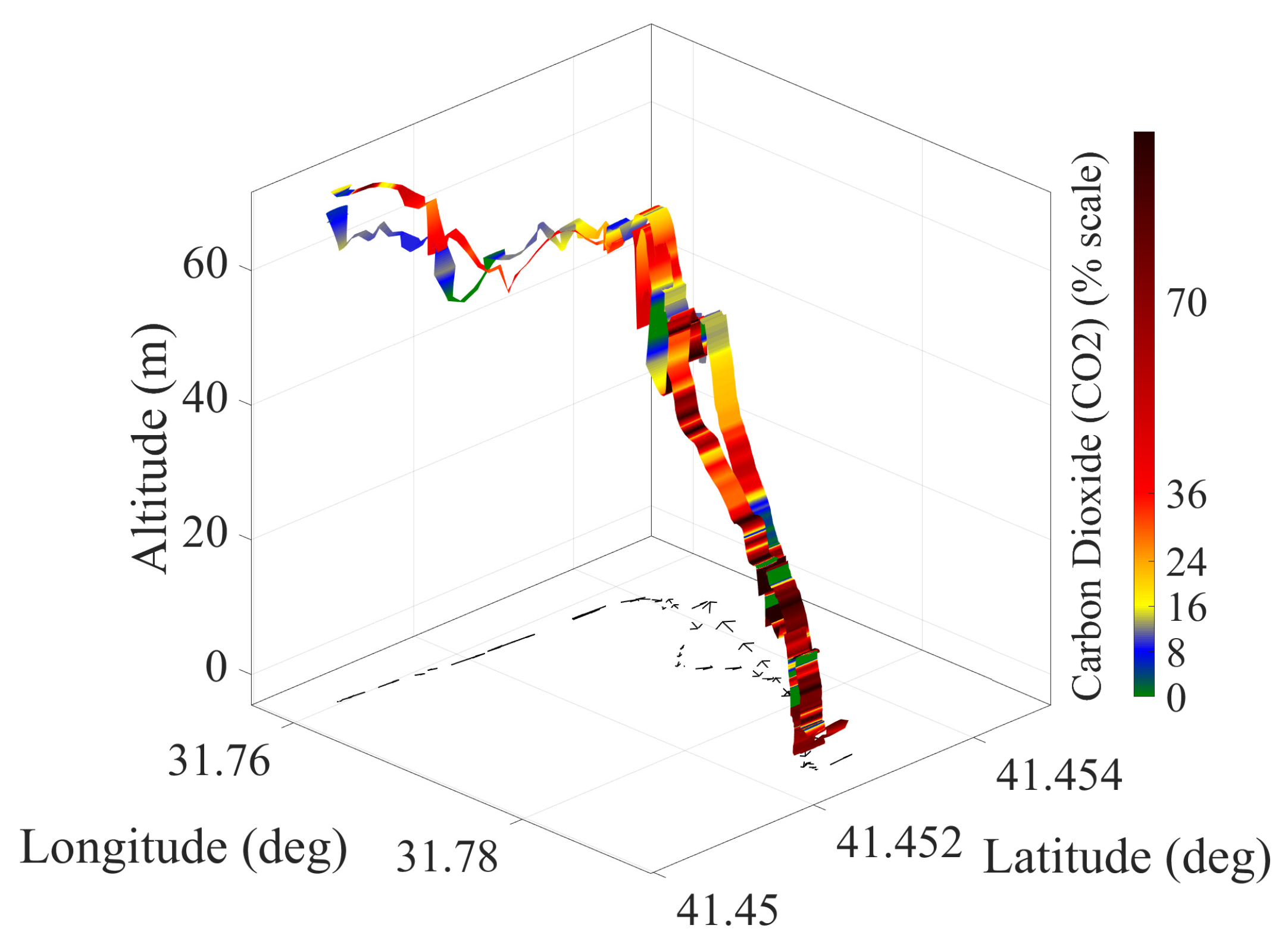
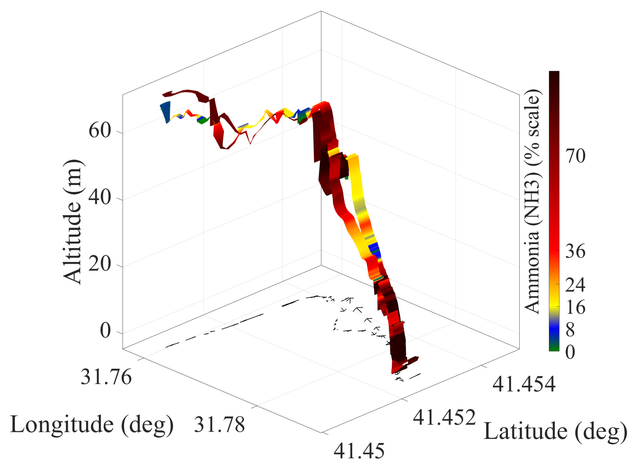
The ten different closed-loop routes are defined to consider road and traffic conditions. The area of these routes is demonstrated in Figure 2 and is located in the city center of Zonguldak/Türkiye. The starting and finishing points, which are the same, are highlighted in Figure 2, and the rough roads and intense traffic conditions are demonstrated. For the Nissan/Juke model vehicle, the emission rates of the specific pollutants of each predefined route are presented in Figure 3. The pollutant emission rates of each route for the Opel/Astra model vehicle are presented in Figure 4. Figure 5, Figure 6 and Figure 7 demonstrate the effect of road characteristics on the emission rates of only Route–1 of the Juke model. The emission rates with the Opel/Astra model are presented in Figure 8, Figure 9 and Figure 10 and seem higher on rough roads and heavy traffic conditions, particularly near traffic lights. However, it cannot be directly confirmed that these pollutants are released at higher rates on rough roads and lower rates on smooth roads, since the variations are not linear depending on the road type. The emissions may be higher than on rough roads, particularly on flat roads, which include heavy traffic and low-speed. To show the vehicle’s descent and ascent on rough terrain, the vehicle’s direction is indicated by arrows at the bottom. Unexpected/high pollutant emission rates can be observed on some flat roads compared to other road types. There are several reasons behind these measurement results: (i) As the speed of the vehicle increases, the aerodynamic drag force of a vehicle and the power demand delivered to the wheel increase at a rate of approximately  P v 3 . Therefore, the fuel consumption per unit distance or  CO 2  production increases. (ii) During high acceleration/overtaking maneuvers, which are more common on flat roads, re-injection transitions may trigger  CO  peaks due to decreased oxidation efficiency. (iii) Under rich operating conditions in a three-way catalyst, side-reaction ammonia leakage ( NH 3  “slip”) can decrease while  NH 3  increases. (iv) Gear ratio and engine speed may push the engine to an inefficient operating point on the map, forcing it to produce the same torque with more fuel and pollutant emissions. Environmental/classification uncertainties such as headwinds, vehicle loads, and small residual slopes on segments classified as flat can increase the effective load demand. These factors, combined with the higher speed/profile fluctuations despite the lower slope of the flat road, consistently explain the higher-than-expected measured emission rates.
As a result, an advanced deep learning technique is preferred for the estimation of pollutant gas emissions, which show nonlinear behavior depending on the road type, vehicle speed, load type, and gear used, and vary depending on many external disturbances. In data training and testing processes, we used the leave-one-route-out (LORO) principle: the first three routes (Routes-1–3), which have 6034 samples, are used only in the training process, while the test data of the other routes (4, 5), which have 4579 samples, are used only for the testing process to obtain an isolated/leakage-safe learning process.

3. Deep Learning-Based Prediction Model

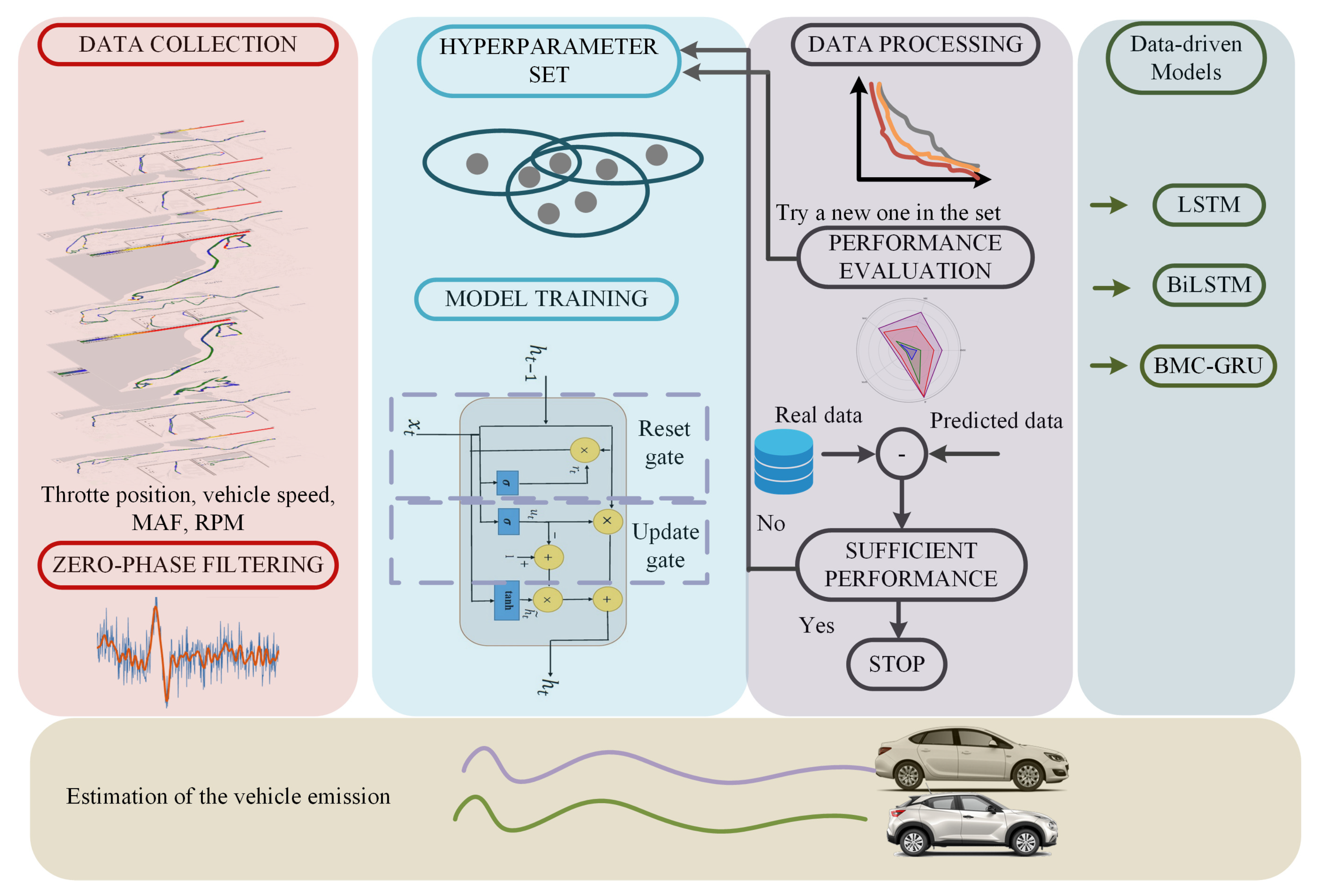
This section introduces the proposed Bayesian Monte Carlo gated recurrent unit (BMC-GRU)-based model training process. To compare the proposed method with state-of-the-art methods, the Ridge regression-based first- and fourth-order one-dimensional polynomials are derived as a combination of throttle position, speed, MAF sensor, and engine RPM of the vehicle. Moreover, a conventional LSTM and a Bidirectional LSTM network are introduced for comparative purposes. The proposed framework of the study is presented in Figure 11.

3.1. Bayesian Method-Based Hyperparameter Optimization

In Recurrent Neural Network (RNN) methods, the hyperparameters of the network are typically defined before the training process using manual research, which requires rerunning the algorithm multiple times. Meta-heuristic optimization methods, i.e., genetic algorithm, gray wolf optimization, and particle swarm optimization, are preferred to investigate a proper hyperparameter set, which dramatically increases the time of the training process [44]. Grid search and random sampling are simple and less time-consuming methods [45]. Bayesian models provide a theoretically sound framework for expressing uncertainty by introducing a probabilistic approach to model parameters. The method searches the posterior distribution, which is given by
p ( φ | D ) = p ( D | φ ) p ( φ ) p ( D ) ,
where
p ( D ) = p ( D | D ) p ( φ ) ,
Over the parameter space  φ  of layer weight vector  W φ D  is the input–output set,  p ( · )  is the probability distribution,  x  is the input vector, and  y  is the output vector. In a classical neural network, each weight  W  is equal to a fixed value, whereas in a Bayesian neural network, a prior distribution  p ( φ )  is assigned to each weight. For a deep learning network, the posterior distribution of the predicted new data  y n + 1  is given by
p ( y n + 1 | x n + 1 , D ) = p ( y n + 1 | x n + 1 , φ ) p ( φ | D ) d φ .
where n is the index of samples. To solve this closed-form expression, posterior computation approximation methods are used in deep networks, i.e., variational inference and a posteriori inference [46]. The approximation method seeks to find an approximate posterior function of the parameter space. The posterior is updated, and the acquisition function is maximized to determine the next hyperparameter vector. The method uses posterior uncertainty to choose new evaluation points and approach the global optimum with few attempts. For a given set of hyperparameters,  θ , the optimal set is given by
θ * = arg max θ l o g p ( D , θ ) .
where  θ *  is the optimal set [47].

3.2. Monte Carlo Dropout Method

The MC-Dropout method is proposed to represent the uncertainty of the deep learning model [48]. The method, which is an approximation of a Gaussian process, offers a simple way to assess network uncertainty without modifying the model structure. The dropout layer is widely included to mitigate the overfitting problem of deep learning networks. However, the weights of the connections to the previous layer are set to zero with an unlearned hyperparameter that has a dropout probability. The approximate posterior function of MC-Dropout is given by
q ( φ ) = 1 n K z n = 0 , 1 δ φ ^ z ( φ ) p z n ( 1 p ) 1 z n q ( z )
where  φ ^  is the learned weights, K is the dimension of the parameter vector,  δ a ( φ )  is the point mass at a, and z is the Bernoulli dropout mask [49]. Substituting  p ( φ , D )  of (3) with (5), the closed form of the MC dropout predictive posterior is given by
p M C ( y n + 1 | x n + 1 , D ) = z { 0 , 1 } K p ( y n + 1 | x n + 1 , φ ^ z ) · q ( z ) .
MC-Dropout enables the use of dropouts before each learning layer and keeps such layers active during inference. The method sets a random dropout probability of the weights to zero each time an inference is made to ensure that different output values are produced [50]. This allows the final estimate and bias to be estimated from multiple iterations.

3.3. Gated Recurrent Unit

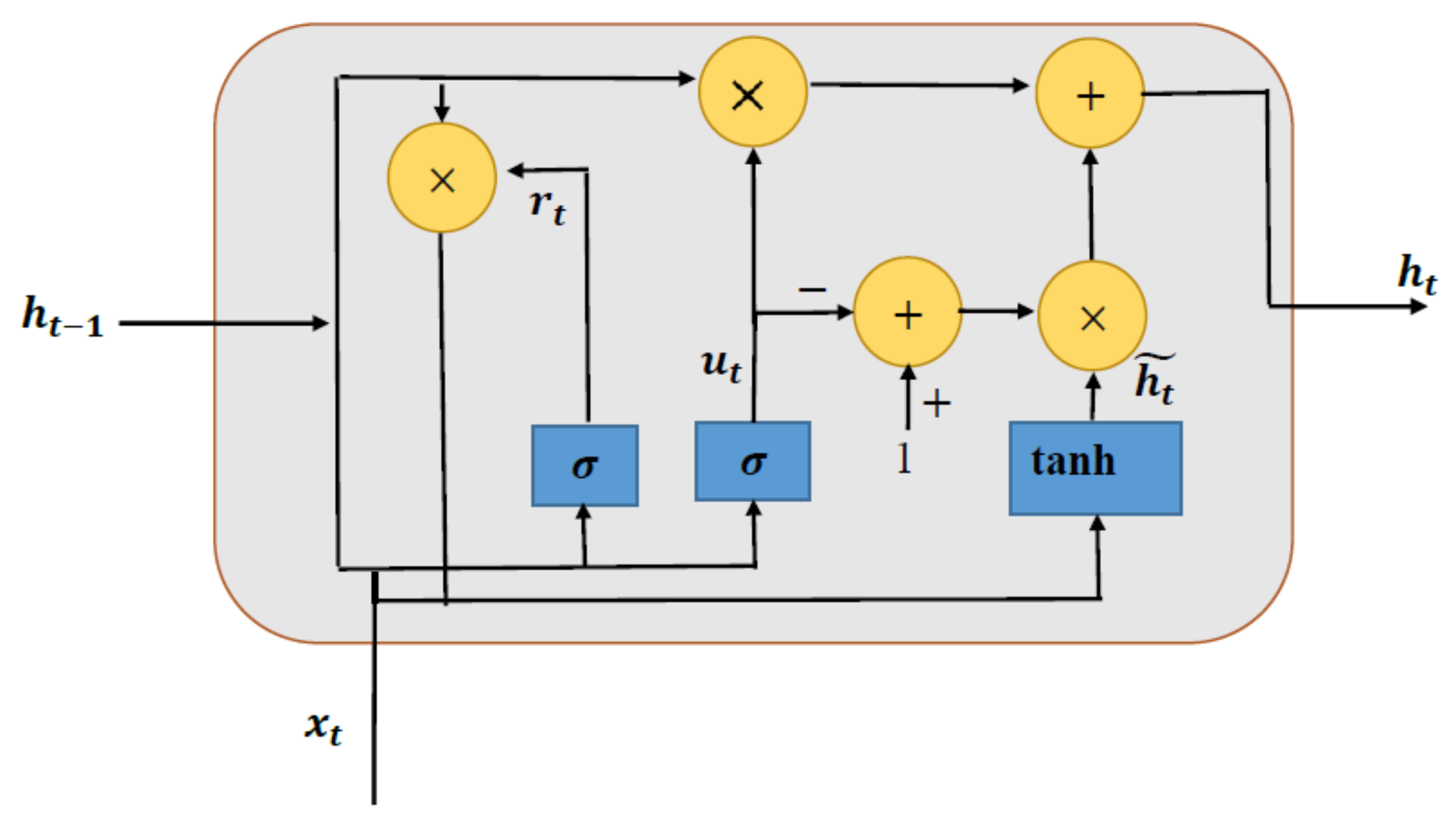
It is observed that the vanishing or exploding gradient problem occurs in the traditional RNN, which makes the deep learning network lose important information during the iterations of the deep learning process. The GRU model was developed to address the gradient problems encountered in RNN models and uses a gate structure to update or delete information from the past during the deep learning process. The GRU is inherently structured with an update gate and a reset gate to solve the gradient problem. The general structure of the GRU-network is presented in Figure 12, where  r t  is the current reset gate,  h t  is the current hidden state,  h t 1  is the previous hidden state,  u t  is the update gate, and  h ˜ t  is the candidate state. The update gate decides the amount of data to keep from the previous hidden state and the amount of information to utilize in the current hidden state. The reset gate specifies the amount of data to be discarded from the previous hidden state. The reset and update gates, respectively, are given as
r t = σ W x r x t + W h r h t 1 + b r ,
u t = σ W x u x t + W h u h t 1 + b u ,
where  σ ( . )  is the sigmoid activation function,  x t  is the input vector,  W x r  is the weight matrix from the input to reset gate  W h r  is the weight matrix from the previous hidden state to the reset gate, and  b r  and  b u  are the bias vectors. The hidden state candidate is given as
h ˜ t = tanh ( W x h x t + W h h r t h t 1 + b h ) ,
where  W x h  is the weight matrix from the input to candidate hidden state,  W h h  is the weight matrix from the previous hidden state to the candidate hidden state,  b h  is the bias vector for the candidate hidden state,  tanh ( . )  is the hyperbolic function, and ⊙ is the element-wise product. The new hidden state is finally obtained as
h t = u t h t 1 + 1 u t h ˜ t ,
where  u t  is the update gate.

3.4. Long Short-Term Memory

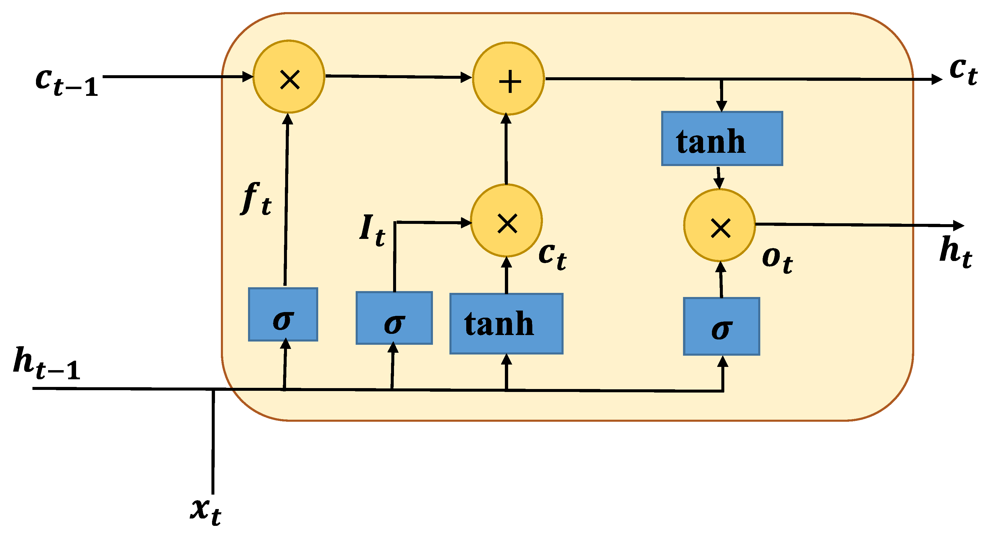
The RNNs can effectively train short-term dependencies in the input data of a deep learning framework [51]. However, some gradient problems in the loss function occur due to long-term dependencies. The layer weights of RNNs cannot be updated, because of a dramatic growth in the gradient. The learning performance of RNNs is negatively influenced by the problems of long-term dependencies. The LSTM network has been introduced to address this indeterminate gradient problem in the backpropagation algorithm [52]. An internal iteration technique without any nonlinear function is used in LSTM networks. The full framework of an LSTM cell is illustrated in Figure 13, where t is the current index of the framework,  c t  is the internal state,  c t 1  is the previous internal state,  h t 1  is the previous hidden state,  x t  is the input pattern,  f t  is the forgetting gate,  i t  is the input gate,  o t  is the output gate,  c ^ t  is the input node,  W h i  is the weight from the hidden gate to the input, and  W x i  is the weight from the input pattern to the input gate. The LSTM cell structure includes three gates: the forgetting, input, and output gates. These gates are defined as
f t = σ ( W x f x t + W h f h t 1 + b f ) ,
i t = σ ( W x i x t + W h i h t 1 + b i ) ,
o t = σ ( W x o x t + W h o h t 1 + b o ) ,
where  ( · )  is the transpose,  σ ( . )  is the sigmoid activation function,  W x f  is the weight vector from the input pattern to the forgetting gate,  W h f  is the weight from the hidden state to the forgetting gate,  W x o  is the weight from the input pattern to output gate, and  W h o  is the weight from the hidden state to the output gate [53]. The terms  b f b i , and  b o  are the bias terms of the specific gates. The sigmoid function in the LSTM framework has been used to constrain the outputs of the gate within  [ 0 ,   1 ] . The forget gate decides which information is excluded from the cell state. The input gate states which new information data is stored in the cell state. The output gate regulates which information is delivered to the cell output based on the current cell state. The input node is defined as
c ˜ t = tanh ( W x c x t + W h c h t 1 + b c ) ,
which is derived from the previous hidden state and input. The hyperbolic tangent function is defined as  t a n h ( · ) . The forgetting and update structure of the memory cell of the LSTM network is denoted as
c t = f t c t 1 + i t c ˜ t ,
where ⊙ is element-wise multiplication. The partial derivative of (15) can be evaluated as
c t c t 1 = c t 1 ( f t c t 1 + i t c ˜ t ) ,
which provides
c t c t 1 = d i a g ( f t ) .
Consequently, the LSTM framework can mitigate the vanishing problems in RNNs. The last main part of the LSTM framework is the output gate, which specifies the cell output [47]. This output gate regulates which information within the LSTM unit is transmitted to the outside. The hidden state of the LSTM unit is defined as
h t = o t tanh ( c t ) .

3.5. Bidirectional LSTM

Bidirectional Long Short-Term Memory (BiLSTM) is a variant of the conventional LSTM and was proposed especially to utilize past and future context information in ordered data [54]. The conventional LSTM framework is introduced to ensure robust performance in ordered data tasks. This LSTM network can learn long-term dependencies in the data. Nevertheless, the learning process in LSTM networks is carried out by utilizing information from the past. The BiLSTM deep learning network could accomplish the learning process by utilizing information from past and future sequences concurrently [55]. The BiLSTM deep learning framework inputs the data to two separate LSTM networks at the same time. One LSTM network processes the sequential data in the forward direction, whereas the other LSTM network simultaneously processes the same data in the reverse direction. Therefore, the BiLSTM network performs a bidirectional learning mechanism in both forward and backward directions at each time step. The forward hidden state in the BiLSTM network is defined as
h t = σ W x h x t + W h h h t 1 + b h ,
where  W x h  and  W h h  are the forward weight matrices, and  b h  is the forward bias vector. The backward hidden state in BiLSTM is defined as
h t = σ W x h x t + W h h h t + 1 + b h ,
where  W x h  and  W h h  are the backward weight vectors, and  b h  is the backward bias vector. As a result, the forward and backward hidden layers in BiLSTM are assessed to enhance the prediction performance [56]. The output of the BiLSTM network is defined as
y t = W h y h t + W h y h t + b y ,
where  W h y  and  W h y  are weights of the output layer from the forward and backward hidden layers, and  b y  is the bias term of network [57].

3.6. Ridge Regression-Based Prediction Model

A feature vector is defined as  x n = [ v n , R P M n , M A F n , p t , n ] R m . A polynomial regression with ridge regularization is given as
y ^ n = β 0 + j = 1 m β j ϕ j ( x n ) .
where m is the number of features, j is the feature index,  { ϕ j ( · ) } j = 1 m  are polynomial features,  β 0  is the bias term of the polynomial, and  β  is the coefficient of the polynomial. A loss function is given as
J ( β 0 , β ) = n = 1 N y n β 0 j = 1 m β j ϕ j ( x n ) 2 + λ j = 1 m β j 2 ,
where N is the number of samples and  λ  is the regularization parameter, which is a nonnegative scalar. The optimal coefficients of the polynomial are given by
( β 0 , β ) = arg min β 0 , β J ( β 0 , β ) .

4. Performance Results of the Data-Driven Estimation Model

This section presents the performance results of the estimation method to evaluate the effectiveness of the proposed methodology. The statistical performance metrics are defined as
RMSE = 1 N n = 1 N y n y ^ n 2 ,
MSE = 1 N n = 1 N y n y ^ n 2 ,
MAE = 1 N n = 1 N y n y ^ n ,
R 2 = 1 n = 1 N y n y ^ n 2 n = 1 N y n y ¯ 2 ,
L o s s = 1 N n = 1 N log cosh y n y ^ n ,
where N is the total number of data points,  y ^ n  is the  n - th predicted value of the model,  y ¯  is the mean of the real values,  c o s h ( x )  is the hyperbolic cosine function, MSE is the mean square error, MAE is the mean absolute error,  R 2  is the coefficient of determination,  L o s s  is the loss function of the deep learning methods, and RMSE is the root-mean-square error.
The hyperparameter set of each deep learning network is given in Table 1. The hyperparameters of the comparison methods are tuned by a manual search method to obtain comparable and leakage-safe settings that consider capacity–generalization balance in emission estimation. The BiLSTM and LSTM networks have a hidden size of 128–128, and a total of four layers (including input/output) is a common “medium-scale” configuration for modeling long-range dependencies while controlling the number of parameters. The dropouts are set to zero for these networks to analyze the pure effect of the baseline architectures and leave regularization as a separate uncertainty mechanism to the BMC component. A learning rate of 0.001 ensures stable and fast convergence for Adam-like adaptive solvers; 60 epochs and 16 batches are used to complete convergence without triggering overfitting on sequences around 10 Hz (limited data, long sequential context) and to limit the GPU memory footprint. In the proposed BMC-GRU, while the same number of layers is maintained, the dropout range [0.1–0.5] is used for uncertainty modeling and calibration, and the learning rate range [ 10 4 10 2 ] is used for convergence/robustness balance. The set of hidden layers is selected as [64–180] to ensure parameter equivalence with LSTM-based comparisons with a width that leverages the parameter efficiency of GRU, using Bayesian search.
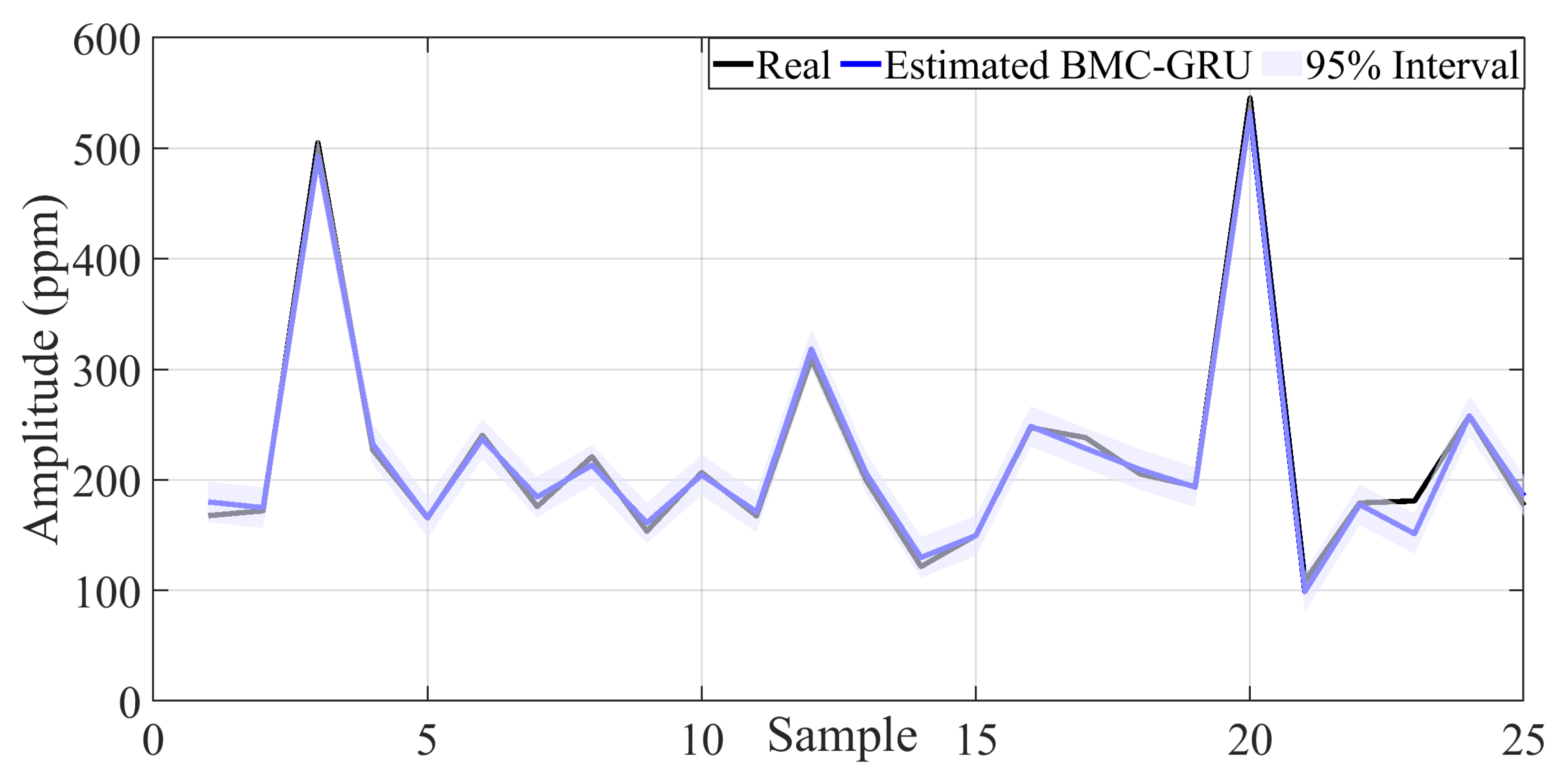
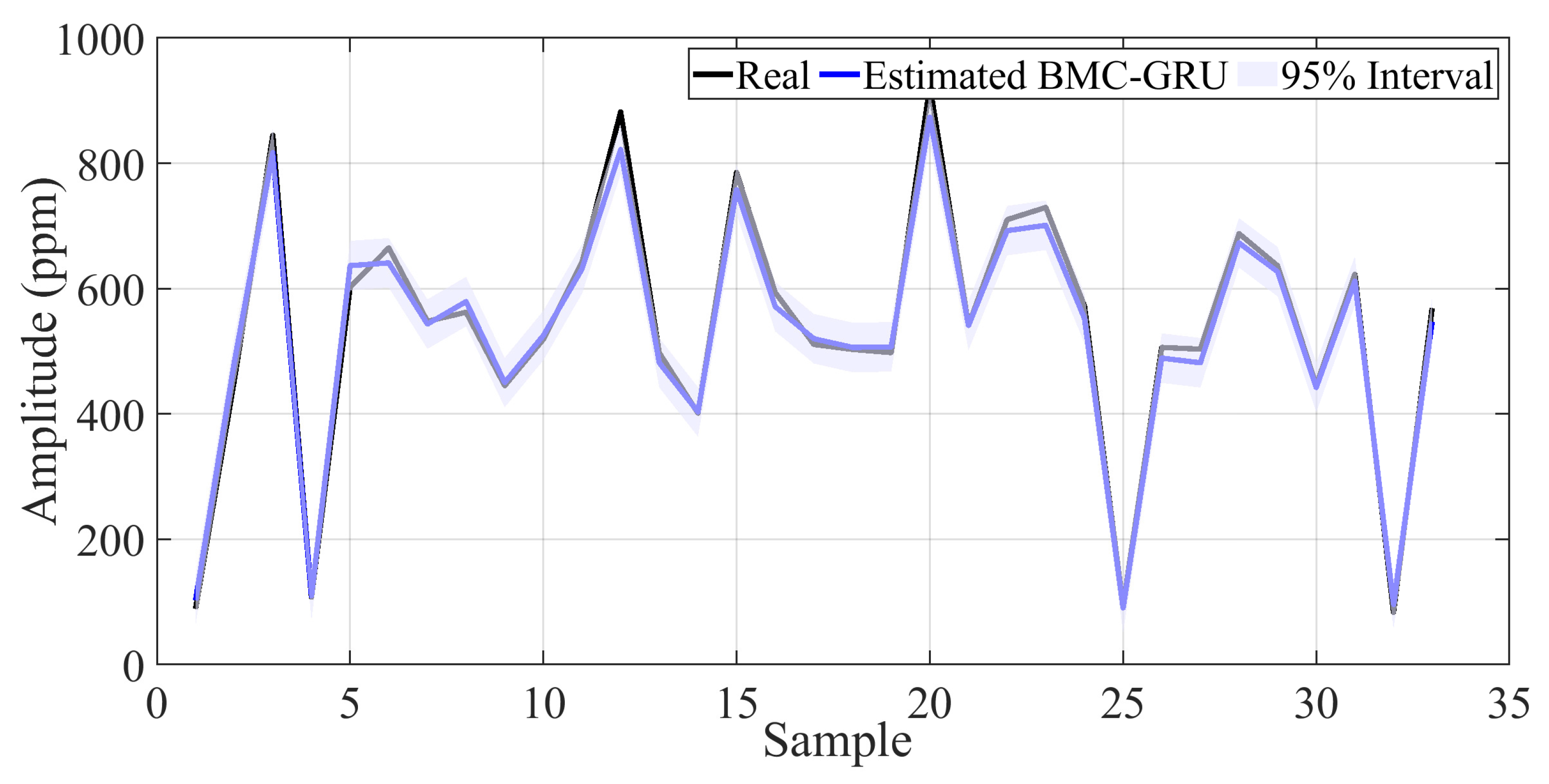
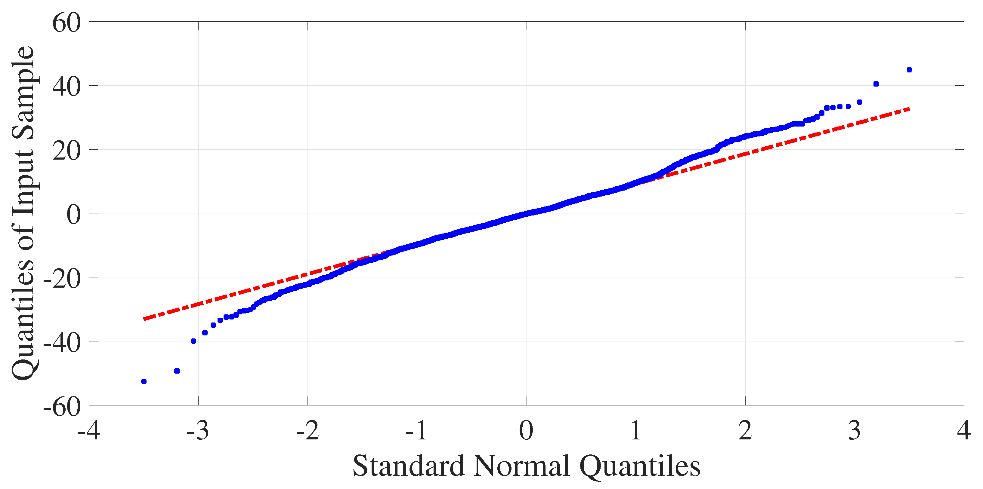
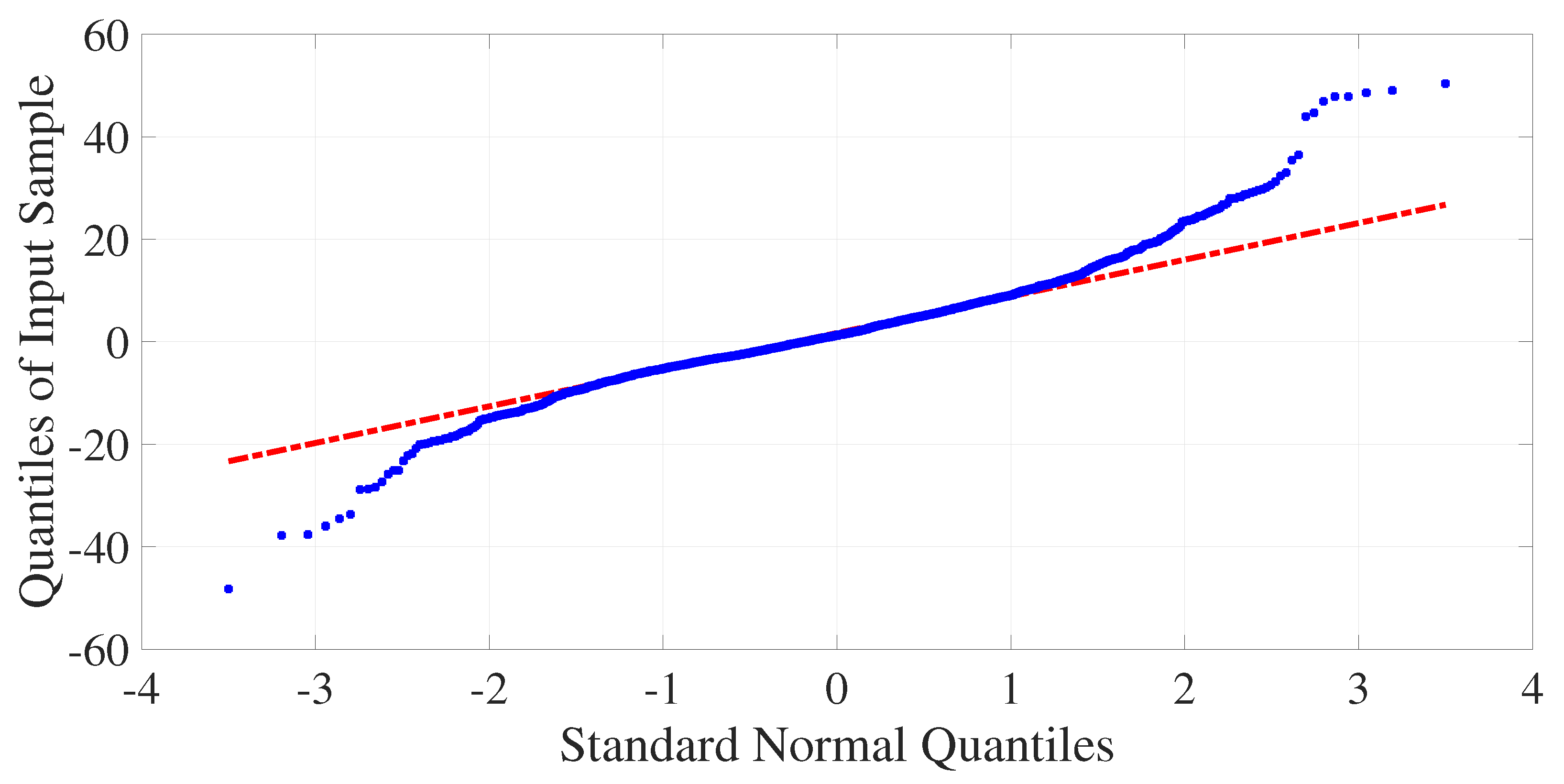
Comprehensive calibration and coverage metrics are used to assess the BMC-GRU deep learning model’s robustness to distribution shifts. In this context, Negative Log-Likelihood (NLL), Prediction Interval Coverage Probability (PICP), and Out of Distribution (OOD) were calculated, and the prediction performance results of the proposed BMC-GRU are included [58,59]. These criteria are tested on the different  CO CO 2 , and  NH 3  pollutant estimations. All metrics of the proposed BMC-GRU deep learning method are given in Table 2. For the  CO CO 2 , and  NH 3  estimation models, the PICP values are 92.5%, 96%, and 93.94%, respectively, which indicates that the proposed deep learning model estimation intervals have high coverage. These findings demonstrate that the confidence interval estimated by the BMC-GRU model includes the vast majority of observed values and is therefore well-calibrated. The NLL values range from 3.63 to 4.49, indicating that the deep learning model estimation probability densities are consistent with the observed distributions, allowing for the avoidance of the over- and under-fitting problems. The OOD ratios range from 4 to 7.5%, demonstrating the proposed deep learning model’s robustness to data outside the training distribution and its overall generalization ability. Specifically, the lowest OOD ratio and the smallest NLL value for the estimation of  CO 2  highlight that the proposed deep learning model has reliable performance under uncertainty for this pollutant. The MC-Dropout calibration analysis of the  CO CO 2 , and  NH 3  estimation models is presented in Figure 14, Figure 15 and Figure 16. These demonstrate the prediction rate of the proposed deep learning model within the  95 %  confidence interval. The proposed BMC-GRU deep learning estimation intervals largely cover the real ppm value. The quantile analysis of the proposed BMC-GRU deep learning model is shown in Figure 17, Figure 18 and Figure 19, where the linear curve represents the closeness of the data to the normal distribution. The blue dots in the curve represent the estimated quantiles of the data set, while the red dashed line indicates the quantiles of the standard normal distribution. The proposed method achieves the presented curves, which are close to the normal distribution in the presented curves.
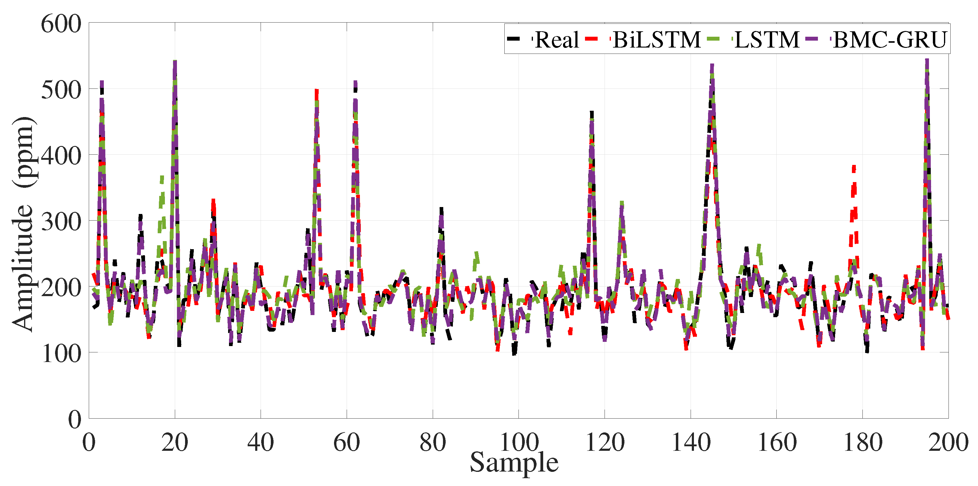
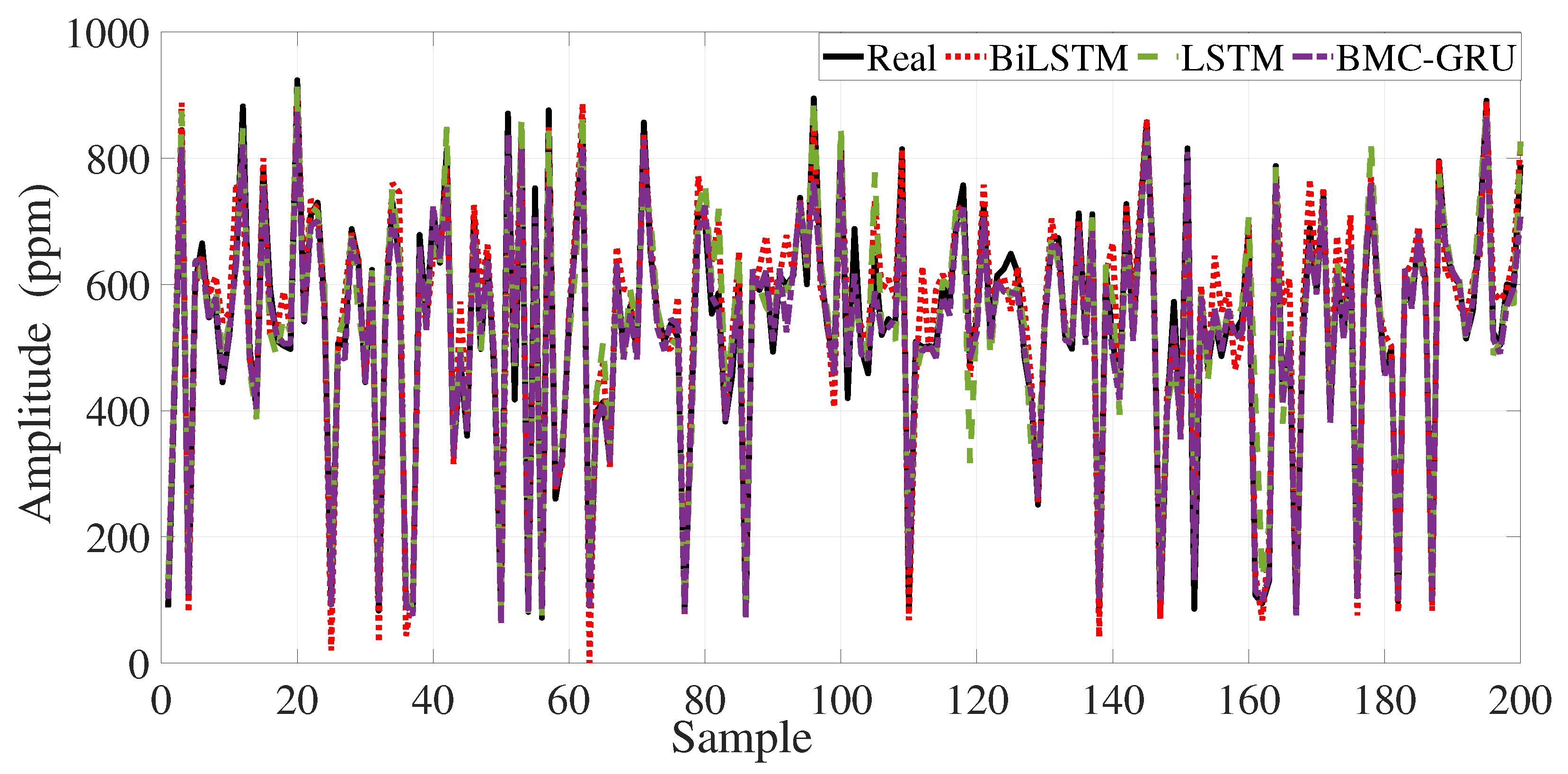
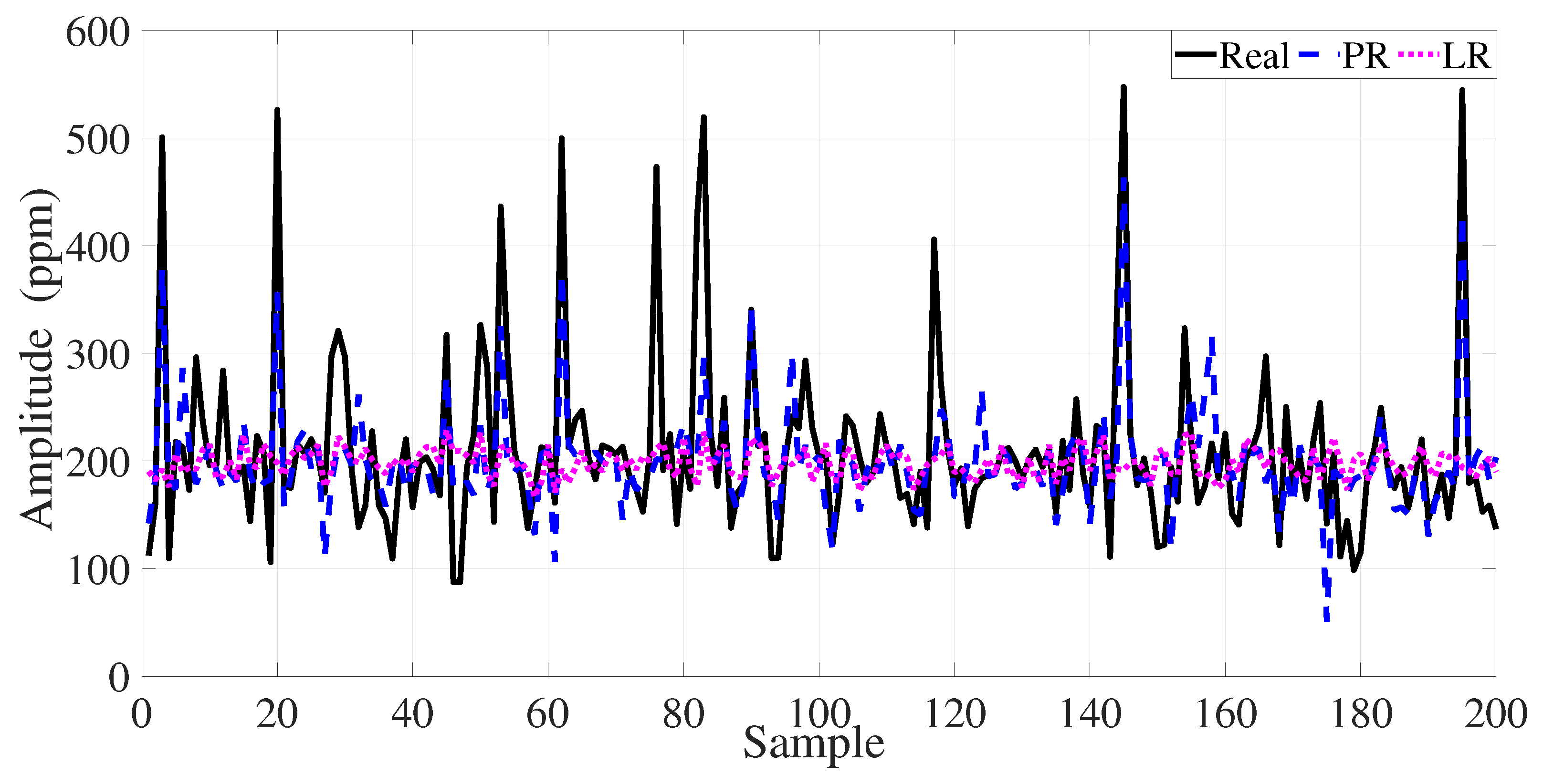
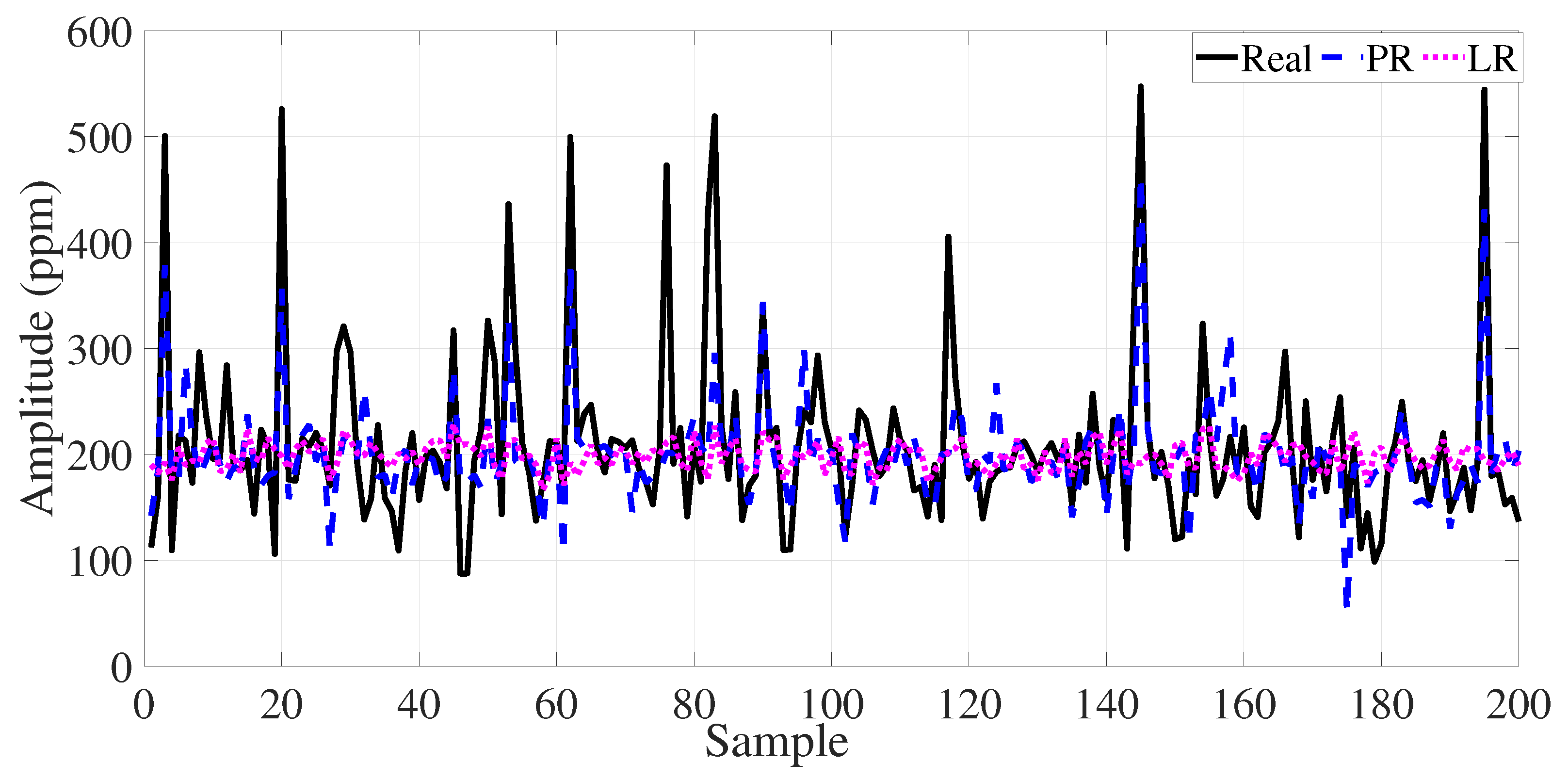
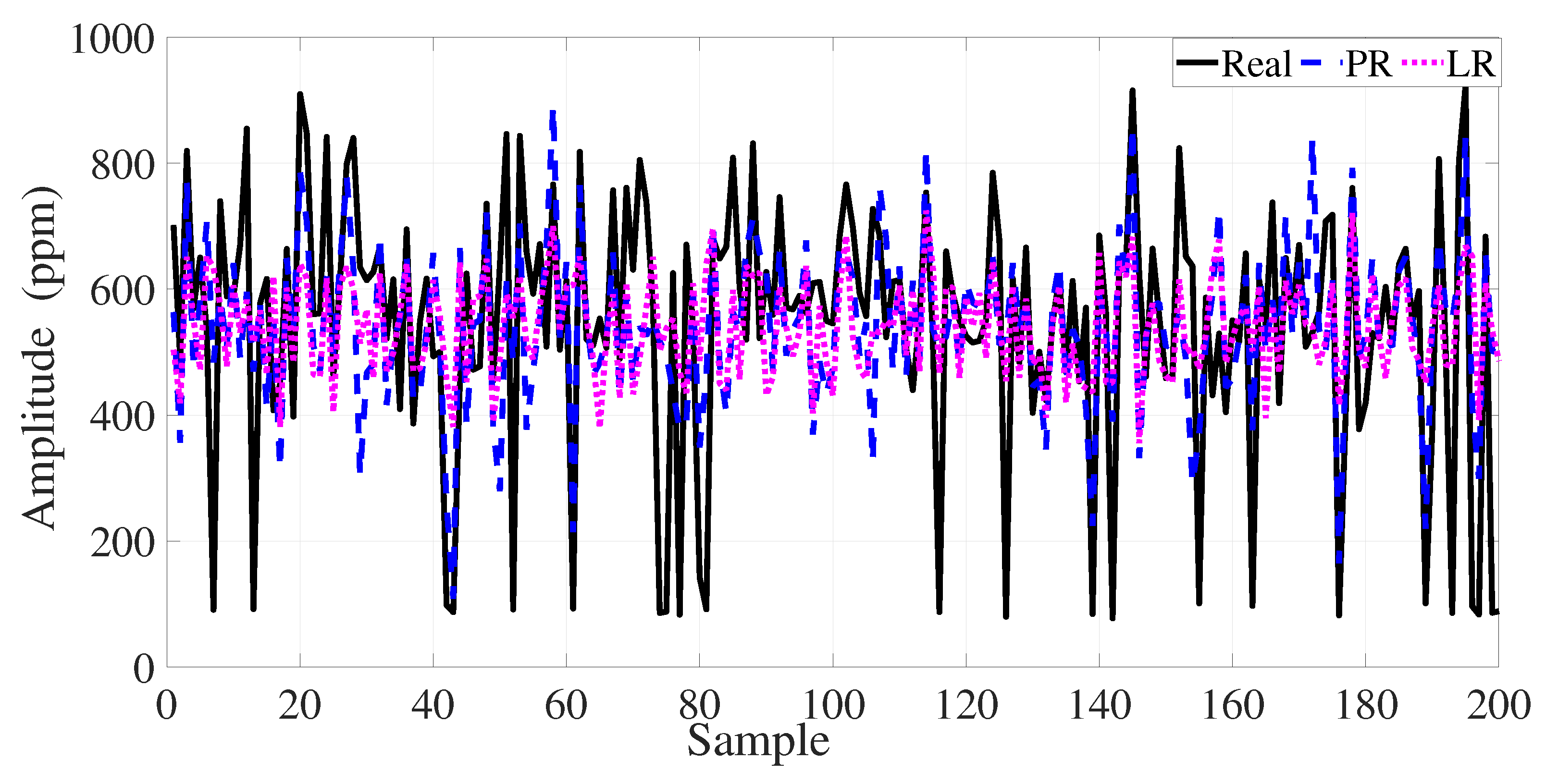
The overall error scores of the deep learning-based networks and the linear ridge-based methods are given in Table 3, which highlights that the proposed BMC-GRU method achieves minimal error metric scores. For CO, BMC-GRU reduced the RMSE value from  27.33  to  10.76  (a decrease of approximately 60.6%) and the  MAE  from  19.43  to  8.16  (a decrease of approximately 58%), while increasing the explained variance from  R 2 = 0.8616  to  0.9785 . For  CO 2 , compared to BiLSTM,  RMSE  improved from  10.67  to  9.20  (a decrease of approximately 13.8%) and  MAE  improved from  7.60  to  6.56  (a decrease of approximately  13.6 % ), while  R 2  increased from  0.9789  to  0.9843 . For  NH 3 , compared to the two-layer LSTM,  RMSE  decreased from  43.85  to  27.09  (a decrease of approximately 38.2%),  MAE  decreased from  30.96  to  19.98  (a decrease of approximately 35.5%), and  R 2  increased from  0.9499  to  0.9809 . Linear and fourth-degree polynomial ridge regression approaches produce high error and low  R 2  for all pollutants (∼0.03–0.40), and BMC-GRU significantly reduces error metrics and demonstrates consistent generalization performance in the  R 2 0.98  range. Finally, the estimation performance of the deep learning network-based models is presented in Figure 20, Figure 21 and Figure 22 for only 200 test data points. The models can track the high-frequency components of real values. The emission estimation performance of regression models is illustrated in Figure 23, Figure 24 and Figure 25, and the pollutant estimation performances of the LR and PR models are compared. These findings indicate that the pollutant estimation performance of the PR model outperforms that of the LR model since the PR has a polynomial of higher degree. However, since these linear regression-based approaches consist of one-dimensional equations, the model success rates they offer are quite low compared to deep learning-based multilayer models.

5. Conclusions

In this paper, a data-driven robust deep learning model based on current state-of-the-art deep Bayesian learning is proposed for vehicle emission estimation, which is based on real-time emission and vehicle parameter ID datasets of multiple vehicles. The Bayesian Monte Carlo Dropout-based gated recurrent unit (BMC-GRU) method-based estimation model presents not only a high-resolution real-time estimation of vehicles on rough country roads, free-flow, and stopped traffic roads but also robustness against network uncertainties during the training process. For benchmarking, several state-of-the-art models are designed using the ridge regression method, LSTM, and BiLSTM networks to evaluate the accuracy of the proposed model on estimating air pollutant concentrations. The proposed BMC-GRU approach outperforms the other estimation models. The  R 2  estimation values of  CO CO 2 , and  NH 3  for the proposed BMC-GRU deep learning approach are given as 0.9785, 0.9843, and 0.9809 scores, respectively. These results show that BMC–GRU exhibits superior performance in time series emission estimation in terms of both accuracy (high  R 2 ) and error metrics ( RMSE MSE MAE ). The method presents a promising solution for uncertainty-aware vehicle emission modeling that can be applicable to transportation systems.

Author Contributions

Conceptualization, R.K., E.B., and S.H.K.; methodology, R.K., E.B., and S.H.K.; software, R.K. and E.B.; writing—original draft preparation, R.K. and E.B.; writing—review and editing, R.K., E.B., and S.H.K. All authors have read and agreed to the published version of the manuscript.

Funding

This work was supported by the Research Fund of Zonguldak Bulent Ecevit University (Project Number: 2025-75737790-01).

Institutional Review Board Statement

Not applicable.

Informed Consent Statement

Not applicable.

Data Availability Statement

The original data supporting the findings of this study is openly available on GitHub at a permanent repository https://github.com/rkeskin/LSTM-GRU-Fuel-consumption-Vehicle-emission-prediction/issues/1#issue-3625340459 (accessed on 9 November 2025).

Conflicts of Interest

The authors declare no conflicts of interest.

References

  1. Hu, X.; Hao, X.; Zhang, K.; Wang, L.; Wang, C. Investigating the effect of estimating urban air pollution considering transportation infrastructure layouts. Transp. Res. Part D Transp. Environ. 2025, 139, 104569. [Google Scholar] [CrossRef]
  2. Mubeen, M.; He, S.; Rahman, M.S.; Wang, L.; Zhang, X.; Ahmed, B.; He, Z.; Han, Y. Smart prediction and optimization of air quality index with artificial intelligence. J. Environ. Sci. 2025, 158, 761–775. [Google Scholar] [CrossRef]
  3. Pan, R.; Zhu, J.; Chen, D.; Cheng, H.; Huang, L.; Wang, Y.; Li, L. Integrated analysis of air quality-vegetation-health effects of near-future air pollution control strategies. Environ. Pollut. 2025, 366, 125407. [Google Scholar] [CrossRef] [PubMed]
  4. Račić, N.; Petrić, V.; Mureddu, F.; Portin, H.; Niemi, J.V.; Hussein, T.; Lovrić, M. A Proxy Model for Traffic Related Air Pollution Indicators Based on Traffic Count. Atmosphere 2025, 16, 538. [Google Scholar] [CrossRef]
  5. Wu, Y.; Zhang, S.; Li, M.; Ge, Y.; Shu, J.; Zhou, Y.; Xu, Y.; Hu, J.; Liu, H.; Fu, L.; et al. The challenge to NO x emission control for heavy-duty diesel vehicles in China. Atmos. Chem. Phys. 2012, 12, 9365–9379. [Google Scholar] [CrossRef]
  6. Ahmed, M.; Zhang, X.; Shen, Y.; Ahmed, T.; Ali, S.; Ali, A.; Gulakhmadov, A.; Nam, W.H.; Chen, N. Low-cost video-based air quality estimation system using structured deep learning with selective state space modeling. Environ. Int. 2025, 199, 109496. [Google Scholar] [CrossRef] [PubMed]
  7. Hao, X.; Hu, X.; Liu, T.; Wang, C.; Wang, L. Estimating urban PM2. 5 concentration: An analysis on the nonlinear effects of explanatory variables based on gradient boosted regression tree. Urban Clim. 2022, 44, 101172. [Google Scholar] [CrossRef]
  8. Smit, R.; Ntziachristos, L.; Boulter, P. Validation of road vehicle and traffic emission models–A review and meta-analysis. Atmos. Environ. 2010, 44, 2943–2953. [Google Scholar] [CrossRef]
  9. Wang, J.; Wang, R.; Yin, H.; Wang, Y.; Wang, H.; He, C.; Liang, J.; He, D.; Yin, H.; He, K. Assessing heavy-duty vehicles (HDVs) on-road NOx emission in China from on-board diagnostics (OBD) remote report data. Sci. Total Environ. 2022, 846, 157209. [Google Scholar] [CrossRef]
  10. Zhao, D.; Li, H.; Hou, J.; Gong, P.; Zhong, Y.; He, W.; Fu, Z. A review of the data-driven prediction method of vehicle fuel consumption. Energies 2023, 16, 5258. [Google Scholar] [CrossRef]
  11. Qu, L.; Wang, W.; Li, M.; Xu, X.; Shi, Z.; Mao, H.; Jin, T. Dependence of pollutant emission factors and fuel consumption on driving conditions and gasoline vehicle types. Atmos. Pollut. Res. 2021, 12, 137–146. [Google Scholar] [CrossRef]
  12. Smit, R.; Dia, H.; Morawska, L. Road traffic emission and fuel consumption modelling: Trends, new developments and future challenges. In Traffic Related Air Pollution and Internal Combustion Engines; Nova Science Publishers, Inc.: New York, NY, USA, 2009; pp. 29–68. [Google Scholar]
  13. Chan, K.; Matthews, P.; Munir, K. Time Series Forecasting for Air Quality with Structured and Unstructured Data Using Artificial Neural Networks. Atmosphere 2025, 16, 320. [Google Scholar] [CrossRef]
  14. Vallamsundar, S.; Lin, J. MOVES versus MOBILE: Comparison of greenhouse gas and criterion pollutant emissions. Transp. Res. Rec. 2011, 2233, 27–35. [Google Scholar] [CrossRef]
  15. Kota, S.H.; Zhang, H.; Chen, G.; Schade, G.W.; Ying, Q. Evaluation of on-road vehicle CO and NOx National Emission Inventories using an urban-scale source-oriented air quality model. Atmos. Environ. 2014, 85, 99–108. [Google Scholar] [CrossRef]
  16. Fujita, E.M.; Campbell, D.E.; Zielinska, B.; Chow, J.C.; Lindhjem, C.E.; DenBleyker, A.; Bishop, G.A.; Schuchmann, B.G.; Stedman, D.H.; Lawson, D.R. Comparison of the MOVES2010a, MOBILE6. 2, and EMFAC2007 mobile source emission models with on-road traffic tunnel and remote sensing measurements. J. Air Waste Manag. Assoc. 2012, 62, 1134–1149. [Google Scholar] [CrossRef]
  17. Kota, S.H.; Ying, Q.; Schade, G.W. MOVES vs. MOBILE6. 2: Differences in emission factors and regional air quality predictions. In Proceedings of the 91st Annual Meeting of the Transportation Research Board, Washington, DC, USA, 22–26 January 2012. [Google Scholar]
  18. Boriboonsomsin, K.; Uddin, W. Simplified methodology to estimate emissions from mobile sources for ambient air quality assessment. J. Transp. Eng. 2006, 132, 817–828. [Google Scholar] [CrossRef]
  19. Jimenez-Palacios, J.L. Understanding and Quantifying Motor Vehicle Emissions with Vehicle Specific Power and TILDAS Remote Sensing. Ph.D. Thesis, Massachusetts Institute of Technology, Cambridge, MA, USA, 1998. [Google Scholar]
  20. Frey, H.C.; Unal, A.; Chen, J.; Li, S. Modeling mobile source emissions based upon in-use and second-by-second data: Development of conceptual approaches for EPA’s new moves model. In Proceedings of the Annual Meeting of the Air and Waste Management Association, Pittsburgh, PA, USA, 22–24 October 2003. [Google Scholar]
  21. Wang, H.; Chen, C.; Huang, C.; Fu, L. On-road vehicle emission inventory and its uncertainty analysis for Shanghai, China. Sci. Total Environ. 2008, 398, 60–67. [Google Scholar] [CrossRef]
  22. Lindhjem, C.E.; Pollack, A.K.; Slott, R.S.; Sawyer, R.F. Analysis of EPA’s Draft Plan for Emissions Modeling in MOVES and MOVES GHG; Research Report# CRC Project E-68; Environ International Corporation: Novato, CA, USA, 2004. [Google Scholar]
  23. Mendes, M.; Duarte, G.; Baptista, P. Introducing specific power to bicycles and motorcycles: Application to electric mobility. Transp. Res. Part C Emerg. Technol. 2015, 51, 120–135. [Google Scholar] [CrossRef]
  24. Liang, Y.C.; Maimury, Y.; Chen, A.H.L.; Juarez, J.R.C. Machine learning-based prediction of air quality. Appl. Sci. 2020, 10, 9151. [Google Scholar] [CrossRef]
  25. Matthaios, V.N.; Knibbs, L.D.; Kramer, L.J.; Crilley, L.R.; Bloss, W.J. Predicting real-time within-vehicle air pollution exposure with mass-balance and machine learning approaches using on-road and air quality data. Atmos. Environ. 2024, 318, 120233. [Google Scholar] [CrossRef]
  26. Wai, K.M.; Yu, P.K. Application of a machine learning method for prediction of urban neighborhood-scale air pollution. Int. J. Environ. Res. Public Health 2023, 20, 2412. [Google Scholar] [CrossRef]
  27. Seo, J.; Lim, Y.; Han, J.; Park, S. Machine learning-based estimation of gaseous and particulate emissions using internally observable vehicle operating parameters. Urban Clim. 2023, 52, 101734. [Google Scholar] [CrossRef]
  28. Azeez, O.S.; Pradhan, B.; Shafri, H.Z. Vehicular CO emission prediction using support vector regression model and GIS. Sustainability 2018, 10, 3434. [Google Scholar] [CrossRef]
  29. Yap, W.K.; Karri, V. ANN virtual sensors for emissions prediction and control. Appl. Energy 2011, 88, 4505–4516. [Google Scholar] [CrossRef]
  30. Azeez, O.S.; Pradhan, B.; Shafri, H.Z.; Shukla, N.; Lee, C.W.; Rizeei, H.M. Modeling of CO emissions from traffic vehicles using artificial neural networks. Appl. Sci. 2019, 9, 313. [Google Scholar] [CrossRef]
  31. Jida, S.N.; Hetet, J.F.; Chesse, P.; Guadie, A. Roadside vehicle particulate matter concentration estimation using artificial neural network model in Addis Ababa, Ethiopia. J. Environ. Sci. 2021, 101, 428–439. [Google Scholar] [CrossRef]
  32. Seo, J.; Yun, B.; Park, J.; Park, J.; Shin, M.; Park, S. Prediction of instantaneous real-world emissions from diesel light-duty vehicles based on an integrated artificial neural network and vehicle dynamics model. Sci. Total Environ. 2021, 786, 147359. [Google Scholar] [CrossRef] [PubMed]
  33. Suri, R.S.; Jain, A.K.; Kapoor, N.R.; Kumar, A.; Arora, H.C.; Kumar, K.; Jahangir, H. Air quality prediction-a study using neural network based approach. J. Soft Comput. Civ. Eng. 2023, 7, 93–113. [Google Scholar]
  34. Antanasijević, D.Z.; Pocajt, V.V.; Povrenović, D.S.; Ristić, M.Đ.; Perić-Grujić, A.A. PM10 emission forecasting using artificial neural networks and genetic algorithm input variable optimization. Sci. Total Environ. 2013, 443, 511–519. [Google Scholar] [CrossRef]
  35. Li, Y.; Jia, M.; Han, X.; Bai, X.S. Towards a comprehensive optimization of engine efficiency and emissions by coupling artificial neural network (ANN) with genetic algorithm (GA). Energy 2021, 225, 120331. [Google Scholar] [CrossRef]
  36. Chang, Y.S.; Chiao, H.T.; Abimannan, S.; Huang, Y.P.; Tsai, Y.T.; Lin, K.M. An LSTM-based aggregated model for air pollution forecasting. Atmos. Pollut. Res. 2020, 11, 1451–1463. [Google Scholar] [CrossRef]
  37. Xie, H.; Zhang, Y.; He, Y.; You, K.; Fan, B.; Yu, D.; Lei, B.; Zhang, W. Parallel attention-based LSTM for building a prediction model of vehicle emissions using PEMS and OBD. Measurement 2021, 185, 110074. [Google Scholar] [CrossRef]
  38. Seng, D.; Zhang, Q.; Zhang, X.; Chen, G.; Chen, X. Spatiotemporal prediction of air quality based on LSTM neural network. Alex. Eng. J. 2021, 60, 2021–2032. [Google Scholar] [CrossRef]
  39. Dalal, S.; Lilhore, U.K.; Faujdar, N.; Samiya, S.; Jaglan, V.; Alroobaea, R.; Shaheen, M.; Ahmad, F. Optimising air quality prediction in smart cities with hybrid particle swarm optimization-long-short term memory-recurrent neural network model. IET Smart Cities 2024, 6, 156–179. [Google Scholar] [CrossRef]
  40. Hu, L.; Wang, C.; Ye, Z.; Wang, S. Estimating gaseous pollutants from bus emissions: A hybrid model based on GRU and XGBoost. Sci. Total Environ. 2021, 783, 146870. [Google Scholar] [CrossRef]
  41. Huang, H.; Qian, C. Modeling PM2. 5 forecast using a self-weighted ensemble GRU network: Method optimization and evaluation. Ecol. Indic. 2023, 156, 111138. [Google Scholar] [CrossRef]
  42. Yang, L.; Ge, Y.; Lyu, L.; Tan, J.; Hao, L.; Wang, X.; Yin, H.; Wang, J. Enhancing vehicular emissions monitoring: A GA-GRU-based soft sensors approach for HDDVs. Environ. Res. 2024, 247, 118190. [Google Scholar] [CrossRef]
  43. Araújo, T.; Silva, L.; Moreira, A. Evaluation of low-cost sensors for weather and carbon dioxide monitoring in internet of things context. IoT 2020, 1, 286–308. [Google Scholar] [CrossRef]
  44. Kanarachos, S.; Mathew, J.; Fitzpatrick, M.E. Instantaneous vehicle fuel consumption estimation using smartphones and recurrent neural networks. Expert Syst. Appl. 2019, 120, 436–447. [Google Scholar] [CrossRef]
  45. Bengio, Y. Practical recommendations for gradient-based training of deep architectures. In Neural Networks: Tricks of the Trade, 2nd ed.; Springer: Berlin/Heidelberg, Germany, 2012; pp. 437–478. [Google Scholar]
  46. Seoh, R. Qualitative analysis of monte carlo dropout. arXiv 2020, arXiv:2007.01720. [Google Scholar] [CrossRef]
  47. Martínez-Ramón, M.; Ajith, M.; Kurup, A.R. Deep Learning: A Practical Introduction; John Wiley & Sons: Hoboken, NJ, USA, 2024. [Google Scholar]
  48. Gal, Y.; Ghahramani, Z. Dropout as a bayesian approximation: Representing model uncertainty in deep learning. In Proceedings of the International Conference on Machine Learning, New York, NY, USA, 20–22 June 2016; pp. 1050–1059. [Google Scholar]
  49. Folgoc, L.L.; Baltatzis, V.; Desai, S.; Devaraj, A.; Ellis, S.; Manzanera, O.E.M.; Nair, A.; Qiu, H.; Schnabel, J.; Glocker, B. Is MC dropout bayesian? arXiv 2021, arXiv:2110.04286. [Google Scholar] [CrossRef]
  50. Padarian, J.; Minasny, B.; McBratney, A. Assessing the uncertainty of deep learning soil spectral models using Monte Carlo dropout. Geoderma 2022, 425, 116063. [Google Scholar] [CrossRef]
  51. Waqas, M.; Humphries, U.W. A critical review of RNN and LSTM variants in hydrological time series predictions. MethodsX 2024, 13, 102946. [Google Scholar] [CrossRef] [PubMed]
  52. Rezazadeh, N.; de Oliveira, M.; Perfetto, D.; De Luca, A.; Caputo, F. Classification of unbalanced and bowed rotors under uncertainty using wavelet time scattering, LSTM, and SVM. Appl. Sci. 2023, 13, 6861. [Google Scholar] [CrossRef]
  53. Ławryńczuk, M.; Zarzycki, K. LSTM and GRU type recurrent neural networks in model predictive control: A Review. Neurocomputing 2025, 632, 129712. [Google Scholar] [CrossRef]
  54. Singla, P.; Duhan, M.; Saroha, S. An ensemble method to forecast 24-h ahead solar irradiance using wavelet decomposition and BiLSTM deep learning network. Earth Sci. Inform. 2022, 15, 291–306. [Google Scholar] [CrossRef]
  55. Sang, S.; Li, L. A stock prediction method based on heterogeneous bidirectional LSTM. Appl. Sci. 2024, 14, 9158. [Google Scholar] [CrossRef]
  56. Peng, S.; Zhu, J.; Wu, T.; Yuan, C.; Cang, J.; Zhang, K.; Pecht, M. Prediction of wind and PV power by fusing the multi-stage feature extraction and a PSO-BiLSTM model. Energy 2024, 298, 131345. [Google Scholar] [CrossRef]
  57. Michael, N.E.; Hasan, S.; Al-Durra, A.; Mishra, M. Short-term solar irradiance forecasting based on a novel Bayesian optimized deep Long Short-Term Memory neural network. Appl. Energy 2022, 324, 119727. [Google Scholar] [CrossRef]
  58. Cui, P.; Wang, J. Out-of-distribution (ood) detection based on deep learning: A review. Electronics 2022, 11, 3500. [Google Scholar] [CrossRef]
  59. Yang, J.; Chen, L.; Chen, H.; Liu, J.; Han, B. Constructing prediction intervals to explore uncertainty based on deep neural networks. J. Intell. Fuzzy Syst. 2024, 46, 10441–10456. [Google Scholar] [CrossRef]
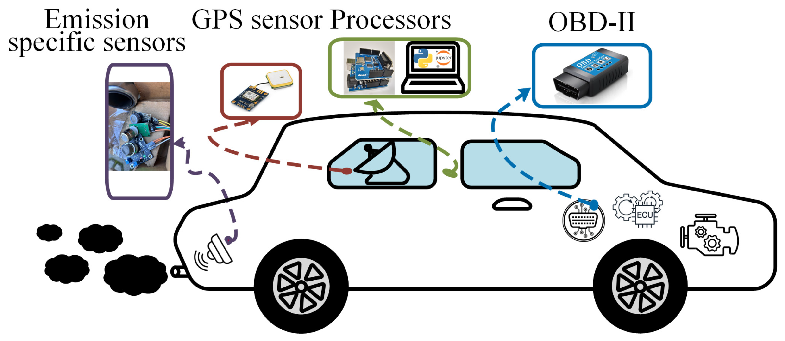
Figure 1. The experimental setup for real-time measurement of the vehicle parameter IDs and specific pollutants.
Applsci 15 12235 g001
Figure 2. The main areas and road conditions of the closed-loop routes for each vehicle.
Applsci 15 12235 g002
Figure 3. The specific emission rates of the Nissan/Juke model vehicle for each pollutant and routes: the left column is for  CO  pollutants, the middle column is for  CO 2  pollutants, and right column is for  NH 3  pollutants, where Routes—(1—5) are labeled as 1—5 and (a, b, c) indicate the spatial distribution of  CO CO 2 NH 3  pollutants, respectively.
Applsci 15 12235 g003
Figure 4. The specific emission rates of the Opel/Astra model vehicle for each pollutant and routes: the left column is for  CO  pollutants, the middle column is for  CO 2  pollutants, and the right column is for  NH 3  pollutants, where Routes—(1—5) are labeled as 1—5 and (a, b, c) indicate the spatial distribution of  CO CO 2 NH 3  pollutants, respectively.
Applsci 15 12235 g004
Figure 5. The vehicle pollutant changes in 3D space for Route—1 of the Nissan/Juke model: The  CO  emission rates in 3D space.
Applsci 15 12235 g005
Figure 6. The vehicle pollutant changes in 3D space for Route—1 of the Nissan/Juke model: The  CO 2  emission rates in 3D space.
Applsci 15 12235 g006
Figure 7. The vehicle pollutant changes in 3D space for Route—1 of the Nissan/Juke model: The  NH 3  emission rates in 3D space.
Applsci 15 12235 g007
Figure 8. The vehicle pollutant changes in 3D space for Route—1 of the Opel/Astra model: The  CO  emission rates in 3D space.
Applsci 15 12235 g008
Figure 9. The vehicle pollutant changes in 3D space for Route—1 of the Opel/Astra model: The  CO 2  emission rates in 3D space.
Applsci 15 12235 g009
Figure 10. The vehicle pollutant changes in 3D space for Route—1 of the Opel/Astra model: The  NH 3  emission rates in 3D space.
Applsci 15 12235 g010
Figure 11. Flowchart representation of the proposed data-driven vehicle emission estimation methodology.
Applsci 15 12235 g011
Figure 12. The full structure of the GRU deep learning model.
Applsci 15 12235 g012
Figure 13. The full structure of the LSTM gates, where the four NN layers are placed in parallel.
Applsci 15 12235 g013
Figure 14. The MC-Dropout calibration analysis of the  CO  estimation model.
Applsci 15 12235 g014
Figure 15. The MC-Dropout calibration analysis of the  CO 2  estimation model.
Applsci 15 12235 g015
Figure 16. The MC—Dropout calibration analysis of the  NH 3  estimation model.
Applsci 15 12235 g016
Figure 17. The quantile—quantile plot of the  CO  estimation model.
Applsci 15 12235 g017
Figure 18. The quantile—quantile plot of the  CO 2  estimation model.
Applsci 15 12235 g018
Figure 19. The quantile—quantile plot of the  NH 3  estimation model.
Applsci 15 12235 g019
Figure 20. The performance of the deep learning network—based  CO  estimation models with real values.
Applsci 15 12235 g020
Figure 21. The performance of the deep learning network—based  CO 2  estimation models with real values.
Applsci 15 12235 g021
Figure 22. The performance of the deep learning network—based  NH 3  estimation models with real values.
Applsci 15 12235 g022
Figure 23. The  CO  emission estimation performance of LR and PR models.
Applsci 15 12235 g023
Figure 24. The  CO 2  emission estimation performance of LR and PR models.
Applsci 15 12235 g024
Figure 25. The  NH 3  emission estimation performance of LR and PR models.
Applsci 15 12235 g025
Table 1. The layers and hyperparameters of the deep learning models.
ModelHidden Layers
(First and Second)
LayersDropoutLearning RateEpochsBatch
Size
BiLSTM128–128400.0016016
2-Layer LSTM128–128400.0016016
BMC-GRU[64–180], [64–180]4[0.1–0.5][0.0001–0.01]6016
Table 2. The metrics of the proposed emission estimation model.
MetricCO   CO 2   NH 3
PICP92.5%96%93.94%
NLL3.883.634.49
OOD7.5%4%6.06%
Table 3. The performance comparison of vehicle emission estimation models.
Pollutant TypeModelRMSEMSEMAE   R 2
  CO BiLSTM31.3839984.947921.81140.8175
2-Layer LSTM27.3329747.085219.42890.8616
PR (4th)57.82953344.246938.42570.3567
LR (1st)70.99235039.904942.53290.0305
BMC-GRU10.7605115.78788.16430.9785
  CO 2 BiLSTM10.6735113.92277.59590.9789
2-Layer LSTM46.95252204.538829.04570.5915
PR (4th)57.82953344.246938.42570.3567
LR (1st)70.99235039.904942.53290.0305
BMC-GRU9.199784.63476.56130.9843
  NH 3 BiLSTM54.11172928.079539.63000.9236
2-Layer LSTM43.84691922.549330.96480.9499
PR (4th)151.162322,850.0524114.99860.4024
LR (1st)176.616131,193.2329134.56480.1842
BMC-GRU27.0893733.828119.97700.9809
Disclaimer/Publisher’s Note: The statements, opinions and data contained in all publications are solely those of the individual author(s) and contributor(s) and not of MDPI and/or the editor(s). MDPI and/or the editor(s) disclaim responsibility for any injury to people or property resulting from any ideas, methods, instructions or products referred to in the content.