Article

Novel Method to Improve the Convergence of Physics-Informed Neural Networks for Complex Thermal Simulations

Laboratoire Génie de Production (LGP), Université de Technologie Tarbes Occitanie Pyrénées (UTTOP), Université de Toulouse, 47 avenue d’Azereix, 65016 Tarbes, France
*
Author to whom correspondence should be addressed.
Appl. Sci. 2025, 15(22), 12234; https://doi.org/10.3390/app152212234
Submission received: 5 October 2025 / Revised: 6 November 2025 / Accepted: 8 November 2025 / Published: 18 November 2025

Abstract

In the context of developing PINN methods for real-time digital twins in manufacturing processes, we propose a new approach that combines two complementary weighting strategies to significantly improve their convergence. The first method, called SD-PINN, balances the loss terms associated with the governing equations, boundary conditions, and initial conditions, ensuring that their contributions are dimensionally consistent and therefore comparable in magnitude. The second method, called SDFEET-PINN, rescales the terms of the governing equations during the early stages of training. This facilitates learning by temporarily modifying the equations to make terms comparable in amplitude, and then progressively restoring the original formulation, thereby preserving the influence of lower-magnitude terms that are often neglected in standard PINN approaches. We apply these methods to transient thermal problems, which are critical for predicting defects in Powder Bed Fusion (PBF). A range of 2D configurations with complex boundary conditions is used to test robustness, and a practical case study is carried out on heat transfer in a complex 3D geometry previously investigated both numerically and experimentally in PBF. Results show that the combined SD-PINN and SDFEET-PINN approach achieves higher predictive accuracy and stability compared to classical PINNs. Furthermore, we introduce an Adaptive Learning Rate strategy that reduces the step size after initial stabilization, further enhancing predictive performance and enabling efficient convergence across all test cases.

1. Introduction

The thermal history of a material is crucial in various thermomechanical processes, particularly in additive manufacturing. In this context, the material is subjected to multiple thermal loads, leading to complex microstructures that significantly affect the performance of the manufactured parts [1,2,3,4]. This study is part of the ongoing development of a digital twin of additive manufacturing, aimed at the real-time correction of manufacturing defects in a closed-loop system.
Figure 1 illustrates the principle of the digital twin of manufacturing processes. On the left, the physical entity (the manufacturing machine) is connected bidirectionally to the virtual entity (the digital twin) on the right. The physical entity is equipped with sensors that capture data, which are then transferred to the “brain” of the virtual entity, i.e., the expert model. This model can incorporate the expertise of metallurgists, tribologists, and data scientists, enabling real-time decision-making without human intervention [5,6]. These decisions may involve adjusting process parameters, such as laser power [7]. In addition to data from physical sensors, it is essential to rely on virtual sensor data provided by simulators, which serve as the digital model of the process [8]. Virtual data help reduce instrumentation costs and provide spatial and temporal information that physical sensors cannot capture. A concrete example of this is the real-time prediction of the microstructure state during the part fabrication process. For instance, no physical equipment currently exists that allows real-time measurement of the microstructure texture of alloys during the Laser Powder Bed Fusion (L-PBF) additive manufacturing process.
Given the challenges associated with digital twin technology, several scientific barriers can be identified:
  • Real-time calculations: To enable real-time decision-making, predictions must be made in real time.
  • Incorporating domain knowledge: The digital twin must integrate domain knowledge such as metallurgy, tribology, numerical analysis, and data science to make informed decisions [9].
  • Online knowledge development: Some information is only available online and must be processed in real time, which creates the challenge of handling large volumes of data.
  • Multi-scale models: The digital twin must cover all scales, from microstructure to machine level, to identify defects.
This project aims to simulate real-time additive manufacturing based on the multi-scale Finite Element approach proposed by Bresson et al. [10] for thermal modeling of L-PBF.
Numerical models often require significant computational time. For real-time calculations, reduction methods (e.g., linearizing equations or relaxing certain assumptions) or surrogate models (such as neural networks, Gaussian processes, polynomial chaos expansions, and more recently, random forests [11]) must be used. Among these tools, neural networks stand out as versatile optimizers, enabling real-time computations and the preservation and transfer of knowledge across various problems. Physics-Informed Neural Networks (PINNs) are particularly effective in extending predictions beyond the initial training ranges of the network [12]. Since the work of Raissi et al. [13], PINNs have gained widespread attention, with numerous studies and dedicated libraries emerging. Despite their advantages, PINNs face significant convergence issues, particularly related to minimizing the loss function, a scalar computed from physical equations, boundary conditions, initial conditions, and sometimes experimental data. As a result, these issues are often addressed on a case-by-case basis.
The balance between physical equations, initial conditions, and boundary conditions has been at the heart of many studies in the literature. The weak form of the physical equations has been used in PINNs by Xu et al. [14] and Rong et al. [15] to reduce the order of the physical equations in relation to the boundary conditions. Other studies have employed arbitrary or adaptive weighting, dynamically adjusting the importance of different terms in the loss function during training. The latter approach has been applied in various studies [16,17,18,19], including the work of Wang et al. [20], which proposes adaptive weighting for solving Navier–Stokes equations. In large deformation problems, Gao et al. [21] also used adaptive weighting to improve model performance. Zhou et al. [16] introduced an auto-adaptive method for large deformation analysis, while Hou et al. [17] discusses adaptive movement of collocation points and adaptive weighting of the loss. Hooshyar and Elahi [22] took a similar approach by sequencing initial conditions in PINNs, progressively adjusting the weights for more accurate results in complex physical scenarios.
Another related approach is Curriculum Learning, where the model is gradually exposed to tasks of increasing complexity [22,23]. For example, Guo et al. [24] used Curriculum Transfer Learning to simulate physical behaviors. The method proposed by Münzer and Bard [25] for progressive collocation point distribution in PINNs is also a related concept, allowing the model to adapt gradually to problem complexity.
The challenges of PINNs are further amplified by the complexities of additive manufacturing [26]. The process itself is challenging to model using numerical approaches, and presents specific challenges for PINNs due to the dynamic changes in the part’s geometry during production. The significant variability in part geometries in Laser Powder Bed Fusion (L-PBF) almost necessitates the development of an individual model for each part.
Only a few studies in the literature have focused on applying PINNs to changing geometries [26,27,28,29]. Recently, Peng and Panesar [26] used PINNs to simulate the layer-by-layer thermal process of the Directed Energy Deposition (DED) additive manufacturing process. The model is 2D with a rectangular geometry and a layer-by-layer sequential approach, where the initial conditions are predicted by a previously trained network. Although the author proposes an extension to 3D, the phenomenon remains almost entirely 2D.
To address these challenges, it is essential to develop advanced PINN models capable of converging effectively despite the complexities of L-PBF additive manufacturing. The existing literature reveals a lack of universally applicable methods. Moreover, most studies simply present results that work without explaining why they work or why others do not. Often, the models are not detailed enough to allow for a comparative study of different approaches.
In this study, we introduce two novel methods for Physics-Informed Neural Networks (PINNs), SD-PINN and SDFEET-PINN, designed to enhance convergence. A new Adaptive Learning Rate strategy is also proposed. Conventional PINNs often face major challenges, such as unbalanced loss terms of different magnitudes, difficulties in handling mixed boundary conditions (Dirichlet, Neumann, and Newton), and poor convergence on complex 3D geometries. The proposed SD-PINN and SDFEET-PINN methods directly address these issues by automatically balancing the different physical loss components and adapting the learning dynamics during training. These improvements lead to faster and more stable convergence and enable accurate predictions in realistic, industrially relevant configurations. The approaches can be used with any method from the literature dealing with the loss function balancing problem. They simply replace classical normalization, which is, in fact, used by all PINN methods. The effectiveness of these approaches is evaluated on four representative problems, including a complex 3D case involving the hydraulic joint studied by Bresson et al. [10] in the context of multi-scale thermal simulation in additive manufacturing. Although the heat conduction equation is relatively simple in its physical formulation, it remains particularly challenging for PINNs when involving mixed boundary conditions (Dirichlet, Neumann, and Newton) and realistic 3D geometries. Such configurations often lead to unbalanced loss terms and poor convergence in standard PINN frameworks. Therefore, this study focuses on improving convergence robustness in these practical but numerically demanding cases. The remainder of the document is organized as follows. Section 2 introduces the proposed methods and their numerical implementation. Section 3 presents the four benchmark problems used for evaluation, along with their numerical formulations. Section 4 discusses the numerical results obtained with the proposed PINN-based approaches, highlighting their robustness and accuracy.

2. Modeling and Methods

2.1. Classical PINN Method

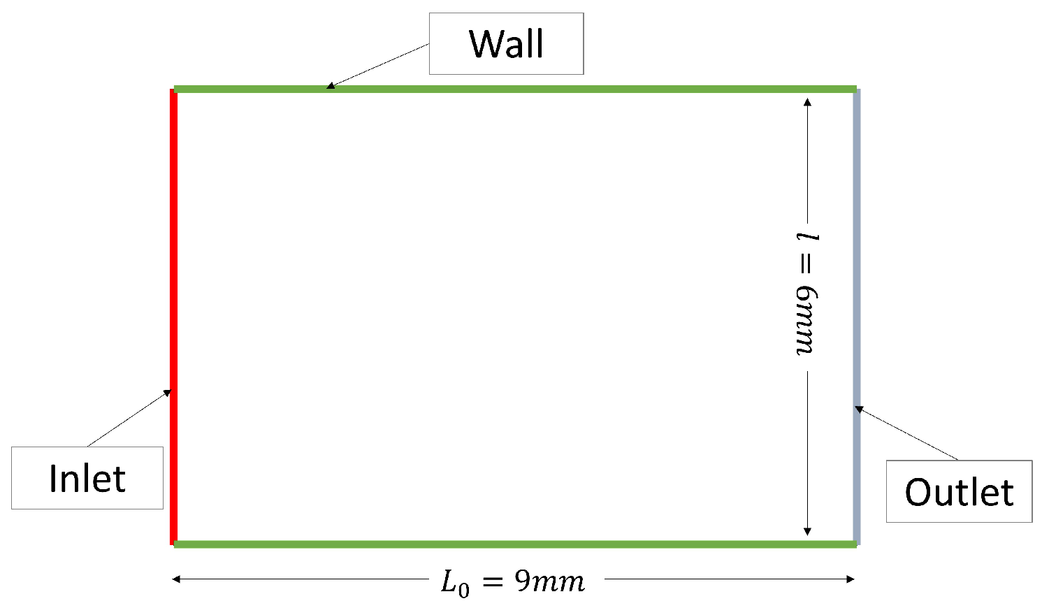
The model’s geometry and the definition of the inlet, outlet, and wall boundaries are shown in Figure 2. The dimensions of the plate are L 0 = 9   m m in length and l = 6   m m in width. The Partial Differential Equation (PDE) for transient heat diffusion is formulated as follows:
ρ c T t = λ 2 T x 2 + 2 T y 2 ( x , y ) Ω , t [ 0 , 1.2 ] T ( x , y , 0 ) = f ( x , y ) ( x , y ) Ω B T = g ( x , y , t ) ( x , y ) Ω , t [ 0 , 1.2 ]
where the density ρ , specific heat c, and thermal conductivity λ are 4210   k g / m 3 , 770   J / k g / K , and 26   W / m / K , respectively. B is a boundary condition operator. For Dirichlet conditions, B T = T on the boundary, while for Neumann conditions, B T = T n on the boundary. The function f ( x , y ) represents the prescribed initial temperature, while g ( x , y ) can represent either a prescribed temperature or flux, depending on the operator B .
The architecture of a standard PINN is shown in Figure 3, where the loss function is composed of losses related to the diffusion equation, L pde , the initial conditions, L ic and the boundary conditions, L in , L out and L wall . The network inputs should also include boundary conditions and other parameters (such as material properties) to enable training with multiple configurations, making it possible to predict any configuration in real-time, even unseen ones [30]. In this work, however, we will restrict the inputs to positions x, y, and time t, as the focus is on validating the new methods rather than real-time computation. For the classical PINN method, Equation (1) is also nondimensionalized, just like the inputs and outputs of the neural networks, in order to maintain the same order of magnitude between the loss functions L pde , L ic , L in , L out and L wall . It should be noted that the neural network architecture used in SD-PINN is identical to that of the standard PINN. The improvement comes solely from the scale-driven normalization of the loss terms, which aligns their physical dimensions and magnitudes, thereby enhancing the stability and convergence of the training process.

2.2. SD-PINN Method

The Same Dimensions PINN (SD-PINN) method is our first approach, based on the non-dimensionalization of the neural network’s input and output variables, as is commonly adopted in the standard PINN method, with the particularity of aligning the physical dimensions of the loss functions for the physical equations, boundary conditions, and initial conditions. Therefore, in the SD-PINN method, we use dimensional equations instead of the non-dimensional ones applied in the standard PINN approach. The preservation of the order of magnitude between the loss functions is achieved by weighting the equations with appropriate coefficients. This approach ensures that the loss functions are of the same physical dimensions, such as power or energy. The selection of these coefficients, which depends on the physical problem and boundary conditions, will be detailed in the various problems discussed in this document.
It is important to note that the proposed weighting ensures that all residuals—those of the governing equation, boundary, and initial conditions—are expressed in the same physical dimension (power). The scaling coefficients are defined so that the residual magnitudes are of the same order, approximately 1% of their characteristic physical terms. This normalization aligns the loss terms, prevents one from dominating the others, and thereby enhances training stability and convergence.

2.3. SDFEET-PINN Method

While the SD-PINN method weights the loss functions, the Same Dimensions From Equal Equation Terms PINN (SDFEET-PINN) method instead weights the terms of the heat equation, as well as those of the initial and boundary conditions, using identical coefficients that gradually evolve toward their true values (corresponding to the coefficient values used in SD-PINN) over the epochs. The distinction between the two methods lies in the use of the From Equal Equation Terms (FEET) strategy in SDFEET-PINN.
In this work, the coefficients evolve linearly toward their true value by the midpoint of the epochs. Consequently, as long as the true coefficient values have not been reached, the FEET strategy temporarily alters the physical problem. However, it helps prevent a term that is initially too small compared to the others from being neglected throughout the training process, particularly in equations with more than two terms.

3. Benchmark Problems for Evaluation

The geometric model illustrated in Figure 2 corresponds to a reference two-dimensional benchmark designed in this study to evaluate the performance of the proposed PINN formulations. It represents a transient heat conduction problem with combined Dirichlet and convection boundary conditions, inspired by standard academic configurations used for validation in thermal analysis. To assess the two proposed methods, various configurations and problem types will be tested. The first group focuses on models with Dirichlet boundary conditions. The second group includes both Dirichlet and Newton boundary conditions, accounting for convective heat exchange with the external environment. The third group extends the second by incorporating an advection phenomenon. Finally, the last group applies the methods to a 3D additively manufactured part that has been extensively studied in experimental and numerical works conducted by Bresson et al. [10,31] and Benoist et al. [32].
To test the ability of our methods to perform under the most challenging conditions, the Adam optimization algorithm is used throughout this study instead of the commonly recommended L-BFGS algorithm for PINNs [33,34]. A simple neural network architecture with six hidden layers of 40 neurons each is employed. The results obtained from the neural network models are compared with those from numerical simulations carried out using the Abaqus finite element software to validate the predictions.

3.1. Problem with Dirichlet Boundary Conditions

Here, we start with a simple problem by applying Dirichlet boundary conditions at the inlet and outlet. To ensure a unidirectional phenomenon, an adiabatic condition is imposed on the wall. This initial problem will allow us to test several activation functions and select the most suitable one for further studies. At the inlet and outlet, temperatures T inlet = 1200   ° C and T outlet = 20   ° C are prescribed, respectively. The initial temperature is set to T initial = 20   ° C , and the total physical simulation time is 1.2   s . With these conditions, the diffusion thermal problem is expected to be constant along the y-direction. Even though the adiabatic condition is imposed on the wall, this problem is referred to as ’Dirichlet boundary conditions’ due to the conditions imposed at the inlet and outlet.
In Equation (1), for Dirichlet boundary conditions, B T = T , and g ( x , y , t ) represents the imposed temperature, while f ( x , y ) is the prescribed initial temperature. For the adiabatic conditions at the wall, B T = T n (where n is the normal outward), with g ( x , y , t ) = 0 indicating no heat flux. Equation (1) then becomes:
ρ c T t = λ 2 T x 2 + 2 T y 2 ( x , y ) Ω , t [ 0 , 1.2 ] T ( x , y , 0 ) = T initial ( x , y ) Ω T ( x , y , t ) = T inlet ( x , y ) Ω inlet , t [ 0 , 1.2 ] T ( x , y , t ) = T outlet ( x , y ) Ω outlet , t [ 0 , 1.2 ] T ( x , y , t ) n = 0 ( x , y ) Ω wall , t [ 0 , 1.2 ]
Introducingresidual errors denoted as R , we define:
R pde ( x , y , t ) = ρ c T t λ 2 T x 2 + 2 T y 2 ( x , y ) Ω , t [ 0 , 1.2 ] R ic ( x , y , 0 ) = T ( x , y , 0 ) T initial ( x , y ) Ω R in ( x , y , t ) = T ( x , y , t ) T inlet ( x , y ) Ω inlet , t [ 0 , 1.2 ] R out ( x , y , t ) = T ( x , y , t ) T outlet ( x , y ) Ω outlet , t [ 0 , 1.2 ] R wall ( x , y , t ) = T ( x , y , t ) n ( x , y ) Ω wall , t [ 0 , 1.2 ]
To normalize the network by making its inputs and outputs dimensionless, we use reference quantities such as temperature T 0 = T inlet , the length L 0 of the model geometry, and the time t 0 = 1.2   s . The new dimensionless variables are expressed as: T * = T T 0 , x * = x L 0 , y * = y L 0 , and t * = t t 0 . Utilizing these new variables, the physical equation transforms into:
ρ c T 0 t 0 T * t * = λ T 0 L 0 2 2 T * x * 2 + 2 T * y * 2
Consequently, the dimensionless equation is derived as:
T * t * = λ ρ c t 0 L 0 2 2 T * x * 2 + 2 T * y * 2
Here, we observe that the non-dimensionalization was carried out by dividing the entire equation by the coefficient of the transient term. We define PINN1, which refers to normalization by the coefficient of the transient term, and PINN2, which refers to normalization by the coefficient of the conduction term.
The Root Mean Square Error (RMSE) of the residuals is expressed as:
L pde = R pde * = T * t * λ ρ c t 0 L 0 2 2 T * x * 2 + 2 T * y * 2 L ic = R ic * = T * T initial T 0 L in = R in * = T * T inlet T 0 L out = R out * = T * T outlet T 0 L wall = R wall * = T * n *
In fact, both dimensional and non-dimensional equations correspond to PDEs of different orders. Dirichlet boundary conditions and initial conditions impose temperature, making them zero-order PDEs, whereas adiabatic boundary conditions impose temperature gradients, which correspond to first-order PDEs. For the heat equation, the conduction term involves second-order temperature gradients, making it a second-order PDE.
With Dirichlet boundary conditions, the residual errors are defined by R * = T * T prescribed T 0 . The acceptable order of magnitude for the value of the residual errors can be deduced from the imposed term T prescribed T 0 , assuming that residual errors are considered acceptable if they are one percent of T prescribed T 0 . For instance, the inlet residual error is acceptable if R in / optimal * = 0.01 T inlet T 0 , which results in R in / optimal * = 0.01 . Furthermore, for the outlet, the residual is considered acceptable when R out / optimal * = 0.01 T outlet T 0 , leading to R out / optimal * = 0.000167 . This reveals a significant difference between the two acceptable residual errors, whose magnitudes can be determined in advance. Moreover, it illustrates how acceptable residual errors from higher-order equations can vary considerably in magnitude. For instance, in the case of the adiabatic boundary condition at the wall, where the residual error is determined by R wall * = T * n * , the acceptable residual error cannot be precisely estimated but is expected to differ significantly from R in / optimal * and R out / optimal * , depending on the physical problem. This highlights the limitations of the classical method in terms of generalizability.
To address this issue, we propose the SD-PINN approach, which expresses initial and boundary conditions in the same physical dimension as the governing heat equation. In fact, the terms in the heat equation, Equation (1), have the dimension of power. The objective is to transform the boundary and initial condition equations so that they are also expressed in terms of power.
In the heat equation, the transient term corresponds to the time derivative of temperature, T t , multiplied by the specific heat c. For prescribed temperature boundary conditions, this derivative can be approximated numerically by considering the residual error T T prescribed as a temperature variation and dividing it by a finite change in time, Δ t . With Δ t chosen such that its order of magnitude reflects a physically acceptable time increment for the discretization of the problem.
Similarly, for Neumann boundary conditions at the wall, the residual error T n 0 , can be divided by Δ l (finite change in length) to compute a numerical second-order temperature gradient, which will then be multiplied by λ ρ to represent the conductive power in the heat equation. Here, Δ l is chosen to be of the same order of magnitude as the mesh element size. Mathematically, this yields:
c T T prescribed Δ t for initial and Dirichlet boundary conditions λ ρ T l 0 Δ l for the Neumann condition at the wall
It is important to emphasize that the expressions in Equation (7) are designed to scale the residuals of the initial and boundary conditions, namely R ic , R in , R out , and R wall , so that they are comparable in magnitude to the terms ρ c T t and λ 2 T x 2 + 2 T y 2 in the heat equation residual R pde , rather than to the residual R pde itself. Since the overall residual R pde of the heat equation is naturally much smaller than its individual terms, the second step involves multiplying the boundary and initial condition residuals ( R ic , R in , R out , and R wall ) by 0.01, under the assumption that the residual of the physical equation can be considered acceptable once it reaches about 1% of its constituent terms. Thus, the residuals for the SD-PINN method are expressed as:
R pde = c T t λ ρ 2 T x 2 + 2 T y 2 R ic = 0.01 c T T initial Δ t R in = 0.01 c T T inlet Δ t R out = 0.01 c T T outlet Δ t R wall = 0.01 λ ρ T n 0 Δ l
or using non-dimensional variables:
R pde = c T 0 t 0 T * t * λ ρ T 0 L 0 2 2 T * x * 2 + 2 T * y * 2 R ic = 0.01 c T 0 Δ t T * T initial T 0 R in = 0.01 c T 0 Δ t T * T inlet T 0 R out = 0.01 c T 0 Δ t T * T outlet T 0 R wall = 0.01 λ ρ T 0 L 0 Δ l T * n *
We define the coefficients C tran , C cond , C ic , C in , C out , and C wall to obtain the following equations:
R pde = C tran T * t * C cond 2 T * x * 2 + 2 T * y * 2 R ic = C ic T * T initial T 0 R in = C in T * T inlet T 0 R out = C out T * T outlet T 0 R wall = C wall T * n *
Hence, SD-PINN loss functions are articulated as:
L pde = C tran T * t * C cond 2 T * x * 2 + 2 T * y * 2 L ic = C ic T * T initial T 0 L in = C in T * T inlet T 0 L out = C out T * T outlet T 0 L wall = C wall T * n *
As previously discussed, Δ t and Δ l should ideally be of the same order of magnitude as the numerical discretization parameters, namely the physical time step and the mesh element size, respectively. However, as a first approximation, and in order to disregard any specific mesh and time discretization, we assume that 1% of the model’s characteristic temporal and spatial scales provides a representative magnitude for the time increment and element size. Accordingly, we set Δ t = 0.01 , t 0 and Δ l = 0.01 , L 0 , which leads to the following coefficient values:
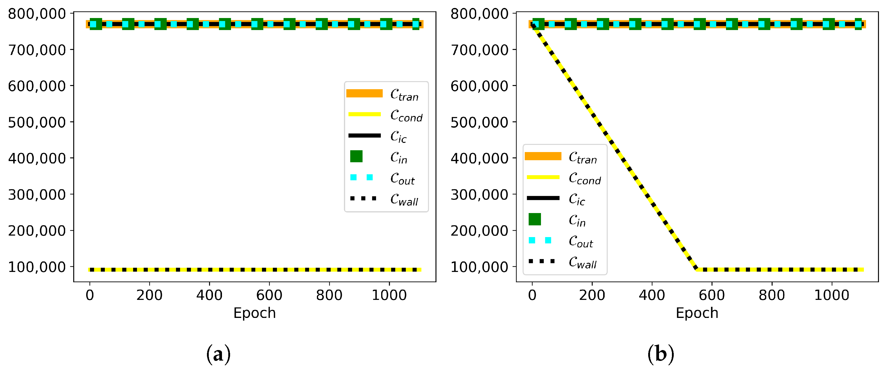
C tran = c T 0 t 0 = 770 , 000 C cond = λ ρ T 0 L 0 2 = 91 , 492.92 C ic = 0.01 c T 0 Δ t = 770 , 000 C in = 0.01 c T 0 Δ t = 770 , 000 C out = 0.01 c T 0 Δ t = 770 , 000 C wall = 0.01 λ ρ T 0 L 0 Δ l = 91 , 492.92
Finally, in the SDFEET-PINN method we propose, the coefficients C tran , C cond , C ic , C in , C out , and C wall vary over the epochs. The idea is to initially assign high importance to each term and then gradually decrease it to its appropriate value. In this work, we have chosen to reach the desired values at half of the total epochs, a point that corresponds to the initial stabilization of the learning process. To determine an appropriate starting value, we compute the maximum coefficient from the heat equation as C max = m a x C tran , C cond and enforce all coefficients to begin at this value until they reach their final values midway through training. Since the true maximum value of the initial and boundary conditions coefficients may exceed C max , we apply a scaling factor of C max m a x C ic , C in , C out , C wall to them. Although this adjustment is not strictly necessary, it ensures that the physical equation dictates the highest coefficient value, resulting in more realistic coefficient values overall.
The evolution of the weighting coefficients implemented for SD-PINN and SDFEET-PINN is presented in Figure 4.
The models, SD-PINN, SDFEET-PINN, PINN1, and PINN2, were trained for 1100 epochs with a network comprising six hidden layers of 40 neurons each. The ADAM optimization algorithm was employed alongside various activation functions, including Exponential Linear Unit (ELU), Sigmoid, and tanh. The learning rate was set to a fixed value of 1 × 10⁻⁴. It is worth noting that in numerical simulations, boundary conditions are strictly enforced in the initial increment. To properly replicate this with neural networks, the initial increment should ideally be divided into multiple steps to accurately describe this evolution. For simplicity, all boundary conditions are interpolated linearly from the initial value to the imposed value over the entire simulation duration. All neural network computations were carried out on an NVIDIA A100-PCIE-40GB GPU server, utilizing the entire set of domain and time points simultaneously, without batching. The computation times for all models are comparable, averaging around 3 min.

3.2. Problem with Dirichlet and Newton Boundary Conditions

The multi-scale L-PBF additive manufacturing model proposed by Bresson et al. [10] simulates the process across various scales, considering the influence of the surrounding powder through Newton boundary conditions. In addition to incorporating these boundary conditions into the model, we start with a warm initial condition of T initial = 1200   ° C to simulate the cooling of the workpiece during additive manufacturing. A Newton boundary condition is applied at the outlet, and a Dirichlet boundary condition with linear cooling to T inlet = 20   ° C is imposed at the inlet. For the Newton boundary condition, the external temperature T e x t is set to decrease from T e x t = 1200   ° C to T e x t = 20   ° C , in accordance with the previously mentioned rule for the progressive application of boundary conditions. To increase the complexity, we use a deliberately high wall heat transfer coefficient of h = 10,000 W m−2 K−1. The physical time is set to 0.3   s .
Only the outlet loss function differs from the previous equations and is expressed as:
L out = 0.01 h ρ T 0 Δ l T e x t T 0 T * 0.01 λ ρ T 0 L 0 Δ l T * x *
The previous output coefficient, C out , is then replaced by two distinct coefficients: one for the heat exchange component, C out / h = 0.01 h ρ T 0 Δ l , and another for the conduction component, C out / k = 0.01 λ ρ T 0 L 0 Δ l . The values of the coefficients are:
C tran = c T 0 t 0 = 3 , 080 , 000 C cond = λ ρ T 0 L 0 2 = 91 , 492.92 C ic = 0.01 c T 0 Δ t = 3 , 080 , 000 C in = 0.01 c T 0 Δ t = 3 , 080 , 000 C out / h = 0.01 h ρ T 0 Δ l = 316 , 706.28 C out / k = 0.01 λ ρ T 0 L 0 Δ l = 91 , 492.92 C wall = 0.01 λ ρ T 0 L 0 Δ l = 91 , 492.92
Here, we also propose a new Adaptive Learning Rate (ALR) approach, which will be compared to a Fixed Learning Rate (FLR) of 1 × 10⁻⁴. The ALR strategy starts training with an initial learning rate of 1 × 10⁻³ and reduces it by half every 100 epochs if the global loss function, L , is higher than its value from 100 epochs earlier. This adjustment strategy is only activated after half of the total epochs have been completed, allowing the model to reach a preliminary convergence before applying learning rate modifications. We maintained the architecture of the previous network but trained it for 10,000 epochs. Once again, the simulation time is comparable across all methods, averaging approximately 25 min.

3.3. Problemwith Advection, Dirichlet, and Newton Boundary Conditions

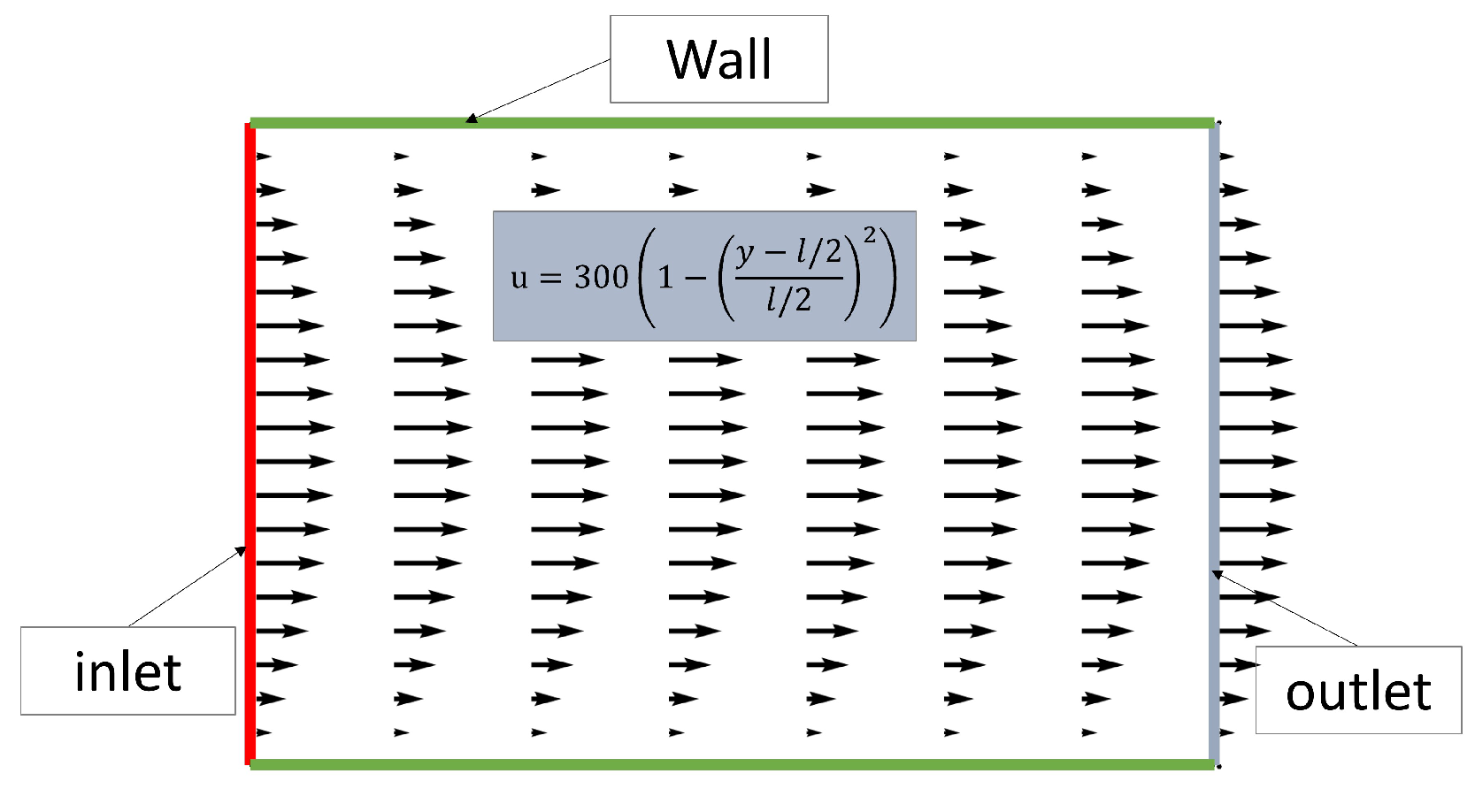
In certain physical problems, the numerical complexity of solving the momentum equation can be circumvented by modeling the material flow using well-established principles. This allows the thermal problem to be solved numerically while incorporating an advection term to account for material movement. As a result, thermal advection can be applied to various thermal problems in fluid mechanics and even in solid mechanics when using the Eulerian formulation. In this subsection, advection has been incorporated into the previous problem. The imposed parabolic advection velocity field is shown in Figure 5. The PDE loss function becomes:
L pde = c T 0 t 0 T * t * + c u max T 0 L 0 u * T * x * λ ρ T 0 L 0 2 2 T * x * 2 + 2 T * y * 2
The coefficients of the heat equation become:
C tran = c T 0 t 0 = 3 , 080 , 000 C cond = λ ρ T 0 L 0 2 = 91 , 492.92 C conv = c u max T 0 L 0 = 30 , 800 , 000
We retained the same network architecture and training for 20,000 epochs. The computation times of the models are similar and are equal to 42 min.

3.4. Application to a Complex 3D Geometry

In this subsection, we apply the methods to a complex 3D geometry. As mentioned earlier, the component used in this study is an additively manufactured hydraulic joint that has been the subject of several numerical and experimental studies. The goal of this project is to replace the multi-scale numerical models for simulating the L-PBF additive manufacturing process, proposed by [10], with neural network-based models for real-time predictions. Therefore, the material data used in this study are derived from the work of [10]. In this case, we focus on the hydraulic joint, considering a macroscopic scale simulation and a specific layer.
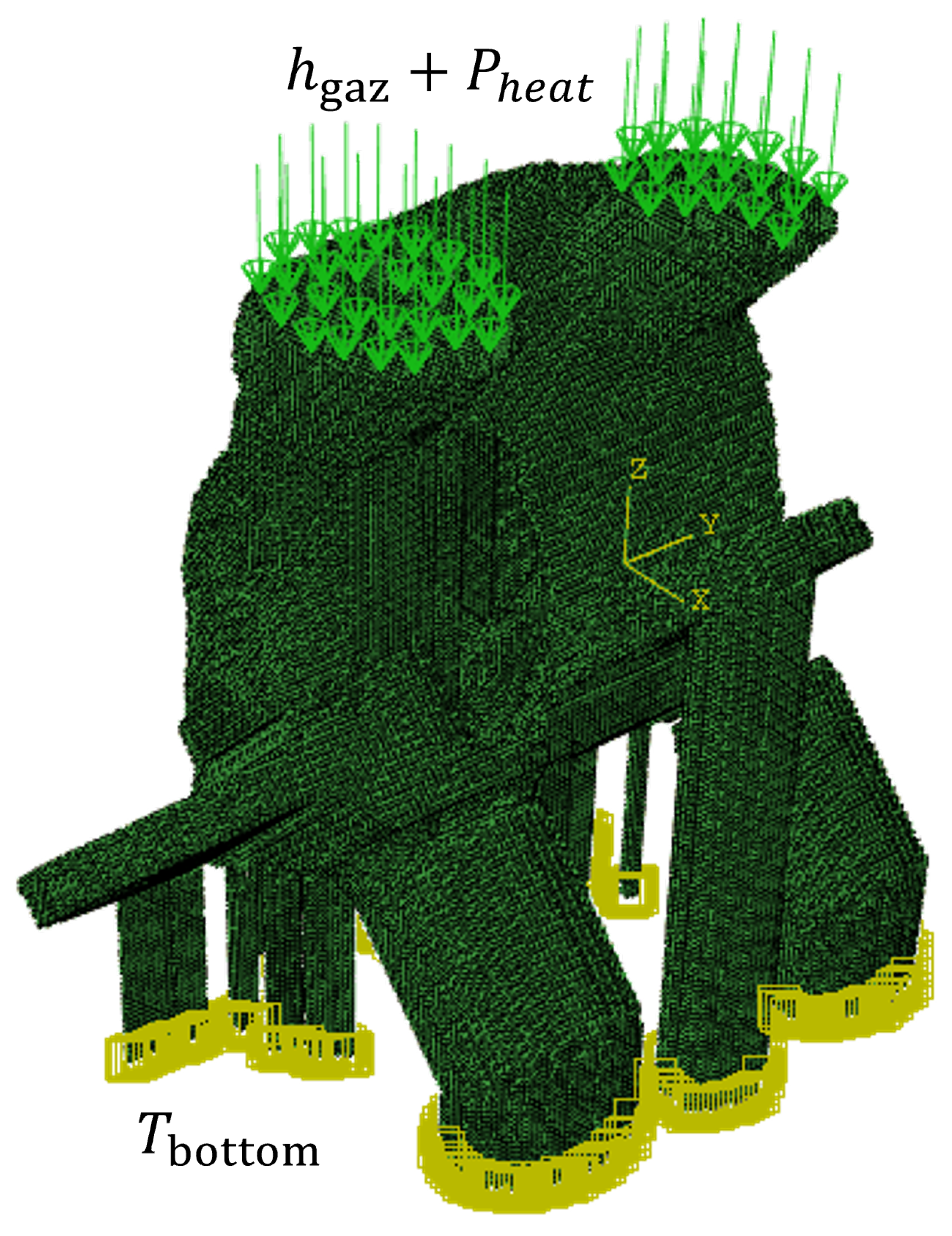
Figure 6 shows the geometry of the part discretized using voxel elements. The bottom of the part is fixed at the plate temperature, T bottom = 170   ° C . The conduction in the surrounding powder that is not explicitly modeled is represented as a convective exchange with a coefficient of h powder = 4   W m 2 K 1 , assuming the powder temperature is equal to the chamber temperature, T ext = 20   ° C . The cooling of the top surface of the part by heat transfer due to the gas flow is represented by a convective exchange with h gas = 200   W m 2 K 1 , with the gas temperature also assumed to be equal to the chamber temperature. A heating flux of P heat = 3000   W m 2 is applied. The physical simulation time is 4 s. All boundary conditions are gradually applied to reach their specified values by the end of the simulation. The loss functions are expressed as follows:
L pde = C tran T * t * C cond 2 T * x * 2 + 2 T * y * 2 + 2 T * z * 2 L ic = C ic T * T initial T 0 L bot = C bot T * T bottom T 0 L pow = C pow / h T ext T 0 T * C pow / k T * n * L top = C top / p + C top / h T ext T 0 T * C top / k T * n *
The coefficients are determined by:
C tran = ρ c T 0 t 0 = 1620.85 C cond = λ T 0 L 0 2 = 12.31 C ic = 0.01 ρ c T 0 Δ t = 1620.85 C bot = 0.01 ρ c T 0 Δ t = 1620.85 C pow / h = 0.01 h powder T 0 Δ l = 0.123 C pow / k = 0.01 λ T 0 L 0 Δ l = 12.31 C top / p = 0.01 P heat Δ l = 46.15 C top / h = 0.01 h gaz T 0 Δ l = 6.15 C top / k = 0.01 λ T 0 L 0 Δ l = 12.31
Due to the large data size, we implemented a strategy that, at each epoch, randomly selects 100% of the initial conditions, 25% of the data from the bottom surface, 5% from the powder surface, 25% from the top surface, and 5% from the internal nodes. This assumption proved acceptable based on the benchmark results. The network was trained for 10,000 epochs. For this part, we consider the three models using the ALR method. The training time for the neural networks is 406 min.

4. Results and Discussions

4.1. Problem with Dirichlet Boundary Conditions

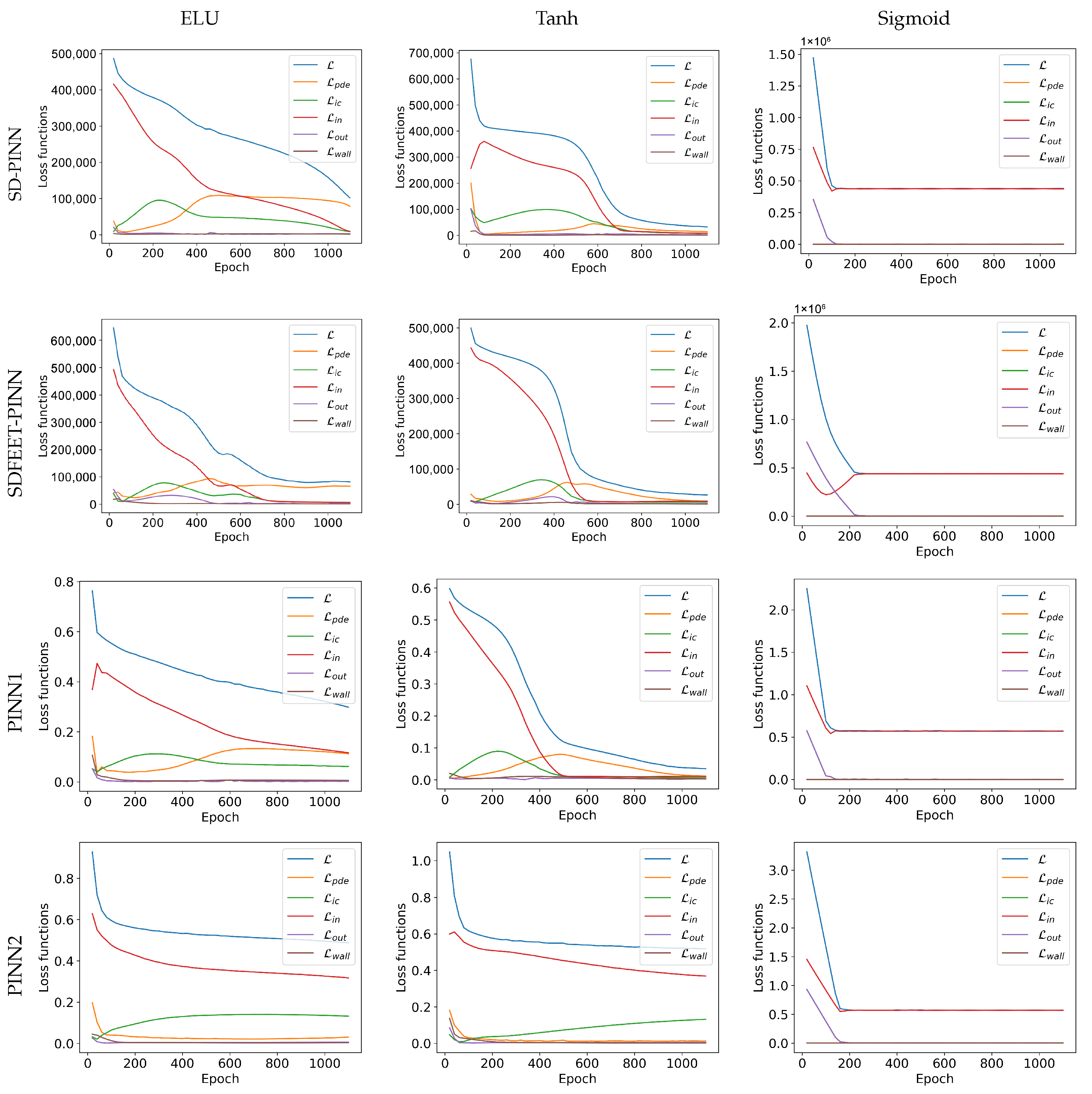
Figure 7 illustrates the loss functions for various activation functions, revealing an interesting competition between them, as some loss functions increase while others decrease. For the Sigmoid activation function, a plateau is quickly reached, with the inlet loss function, L in , being significantly more dominant than the others. This plateau can be attributed to the characteristics of the Sigmoid activation function, which approaches zero for input values less than zero. Although all domain point coordinates are positive, the inlet’s x-position is zero, bringing it closer to the influence of the vanishing part of the Sigmoid function. However, the inlet loss function remains predominant in the graphs of other activation functions as well, but converges more effectively, particularly with the tanh activation function. That being said, this observation should be interpreted with caution, as the rapid convergence of a loss function does not necessarily indicate good predictive performance.
To further analyze the predictions, we plotted the dispersion of prediction errors for the different models in Figure 8. It is clearly visible that the predictions are poor for both the Sigmoid activation function and the PINN2 method. With the PINN1 method, only the tanh function performs well. With our two new methods, SD-PINN and SDFEET-PINN, the results are strong, except for the Sigmoid function, which, in any case, performs poorly across all methods.
These results indicate that our two methods, SD-PINN and SDFEET-PINN, achieve better performance and that the tanh activation function is the most effective. The tanh function was, therefore, retained for all subsequent simulations, as it provides smooth and symmetric gradients (ranging from −1 to 1) that favor the computation of higher-order derivatives required by the physical equations while ensuring stable convergence. This observation is also consistent with many recent studies in the PINN literature.
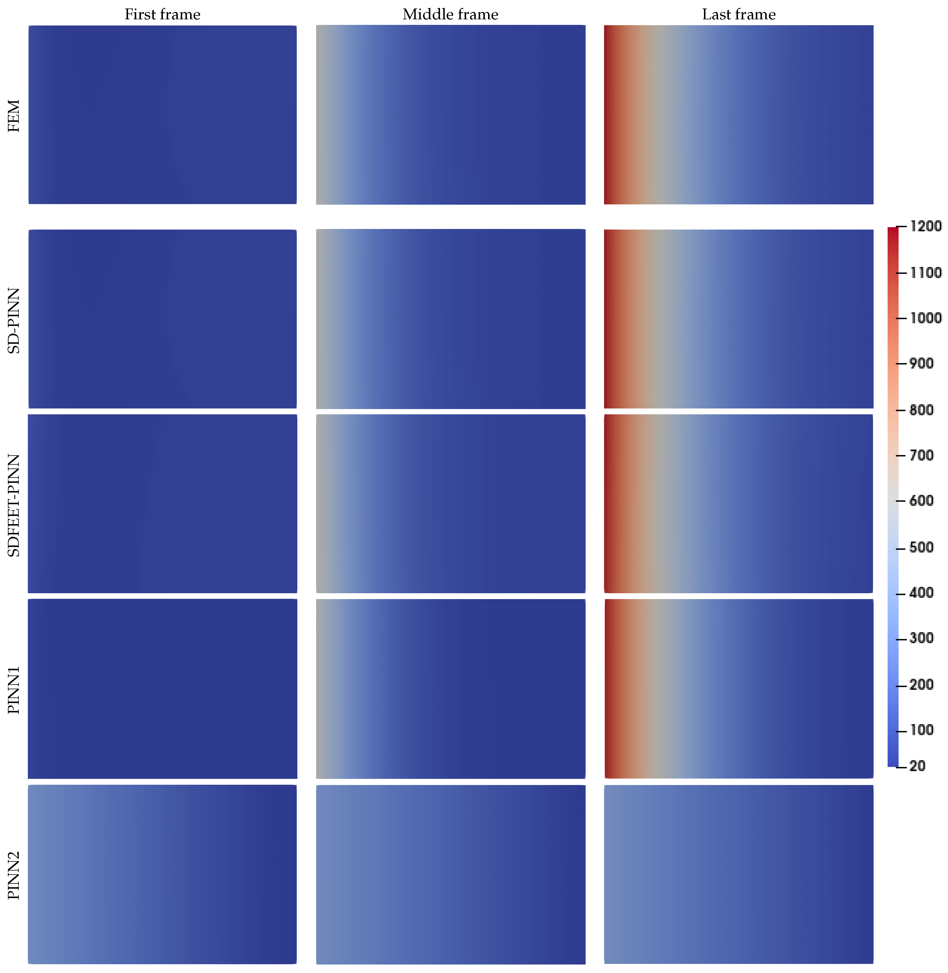
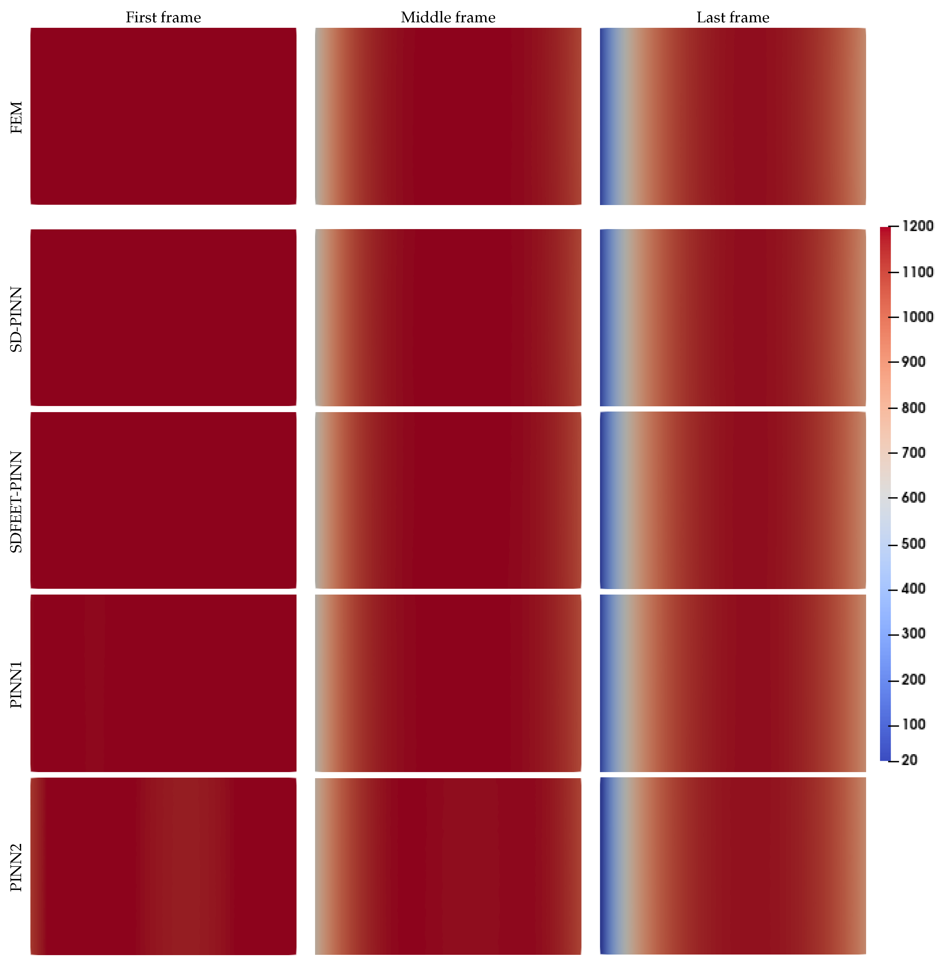
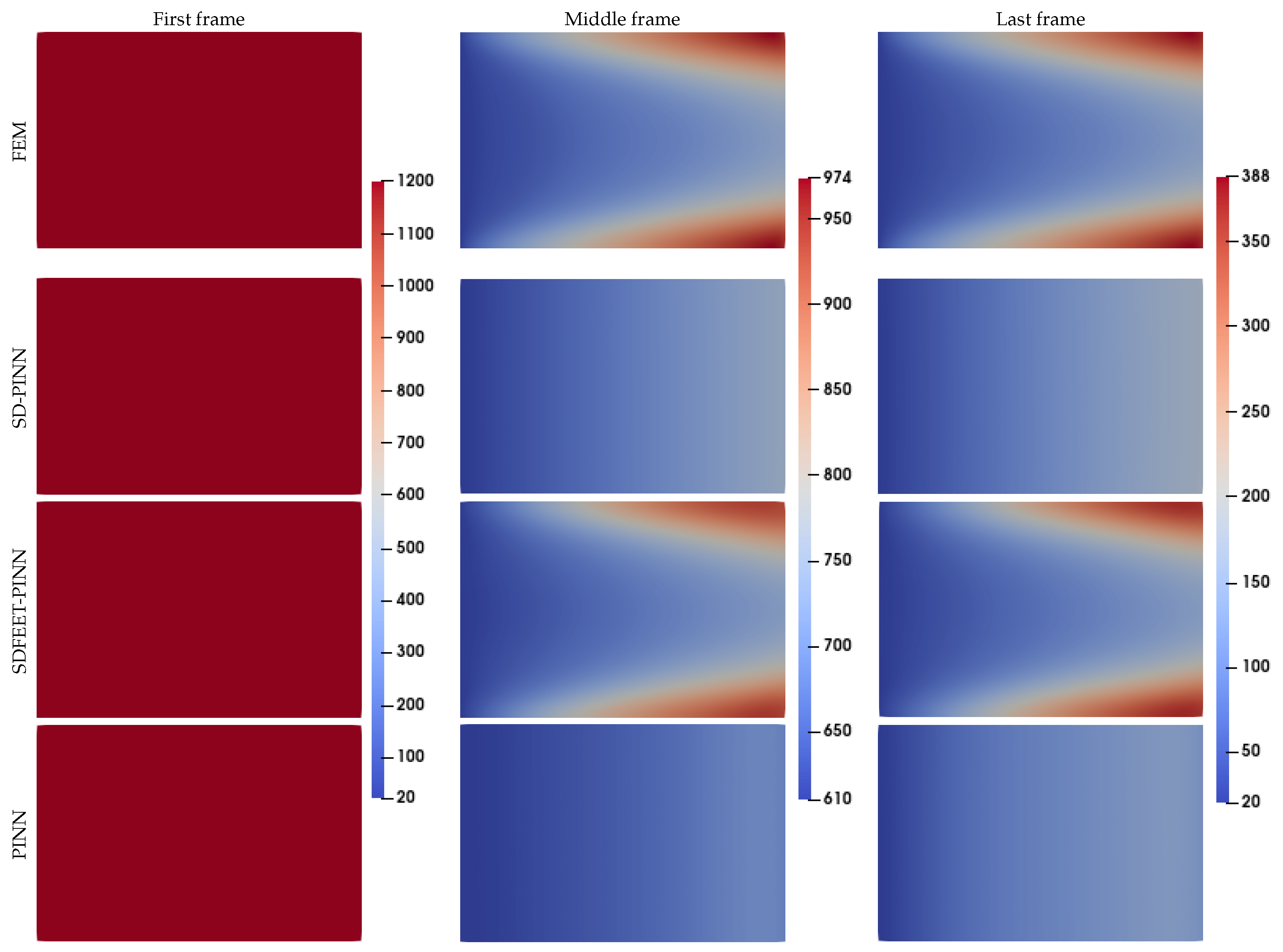
The temperature fields obtained from all methods were compared to the numerical simulation results, as shown in Figure 9. The initial, middle, and final frames are presented. The predictions appear satisfactory, except for the PINN2 method, which confirms the poor performance observed in the tanh dispersion graphs in Figure 8.
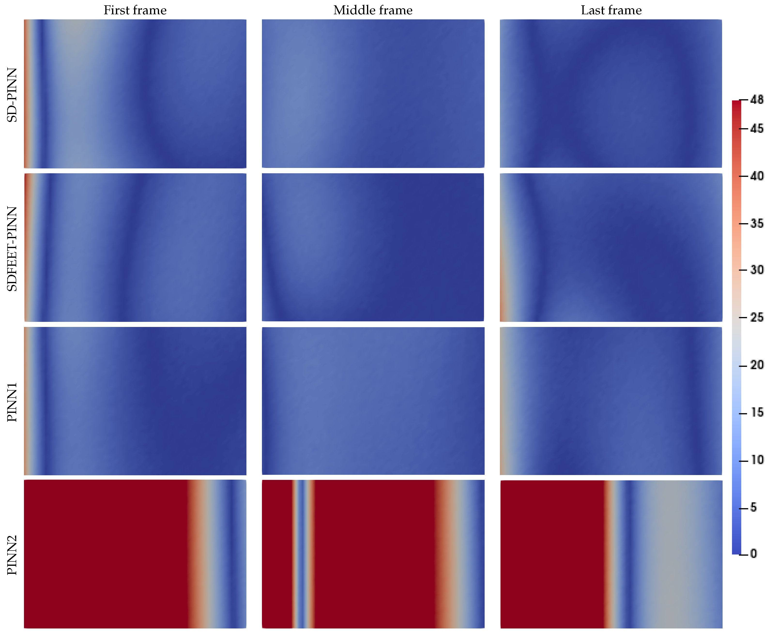
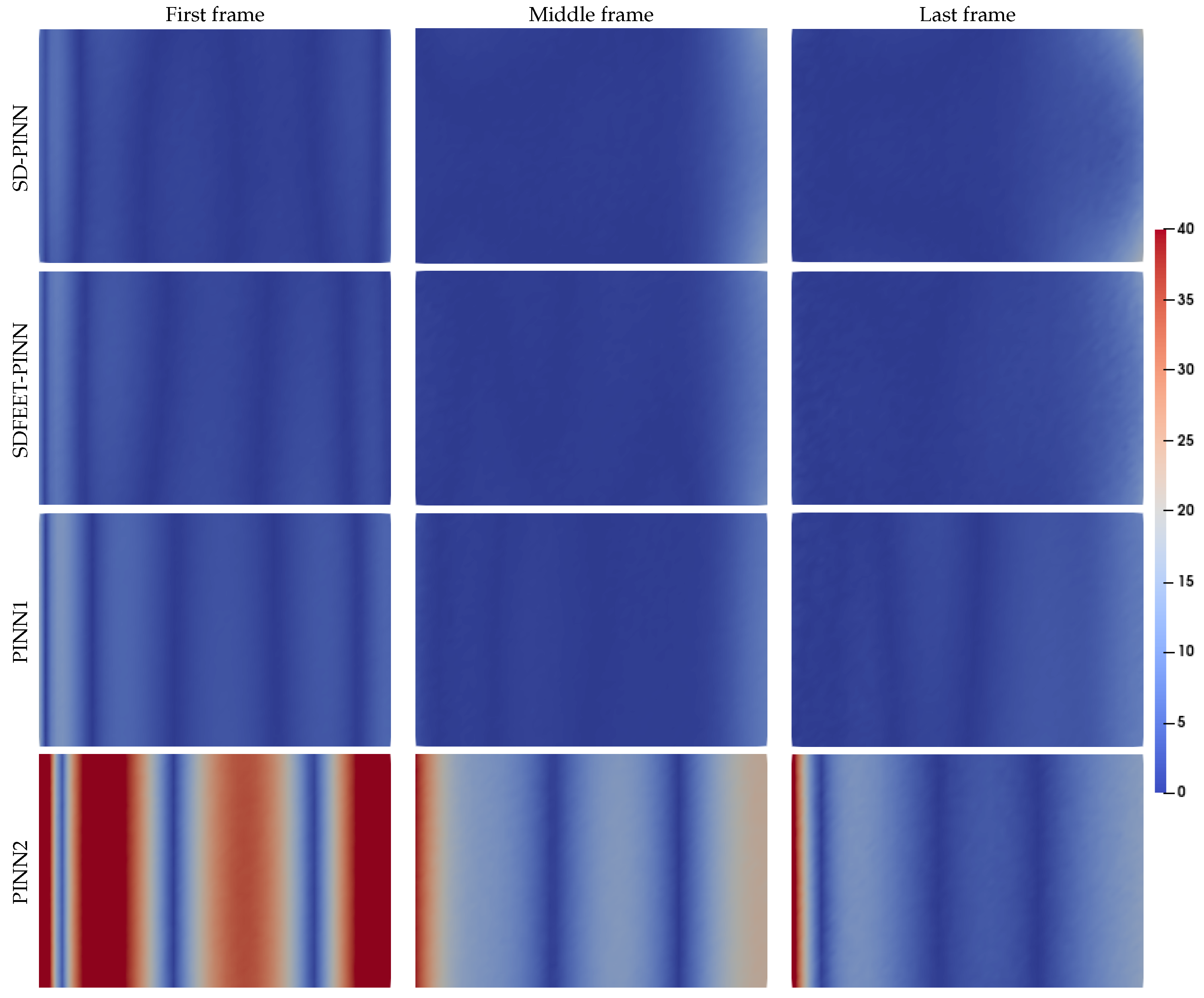
To gain further insights, the absolute error of the thermal field is presented in Figure 10, highlighting significant discrepancies between the predictions of the PINN2 method and the numerical results. For the other methods, SD-PINN, SDFEET-PINN, and PINN1, the maximum absolute error is around 45   ° C and is clearly localized at the inlet. This aligns well with the dominance of the inlet loss function, L in , in the loss graphs shown in Figure 7.
Moreover, an absolute error of 45 ° C represents a large deviation at low temperatures, particularly in regions where the temperature is close to 20 ° C . This can be explained by the fact that the network was trained using absolute error metrics (RMSE or MSE), while the temperature range under consideration spans from 20 ° C to 1200 ° C . This choice is deliberate, since the influence of low-temperature regions on the quantities of interest is negligible. For instance, the alloy microstructure is not affected by deviations on the order of 45 ° C at low temperatures (below 300 ° C ). Consequently, throughout this work, absolute error measures are consistently adopted, as the networks are trained with absolute error-based losses (RMSE and MSE), which makes them more relevant than relative errors.

4.2. Problem with Dirichlet and Newton Boundary Conditions

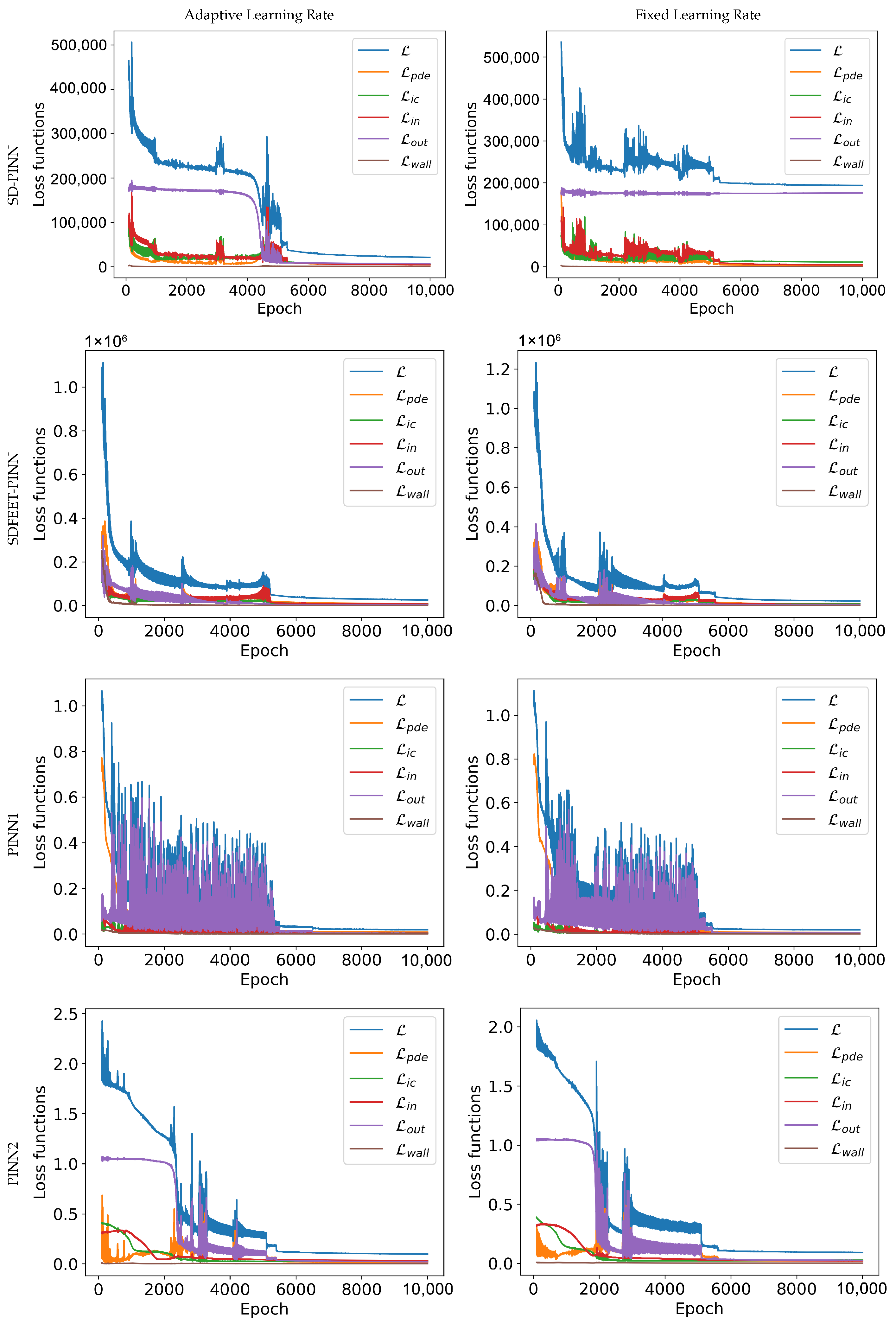
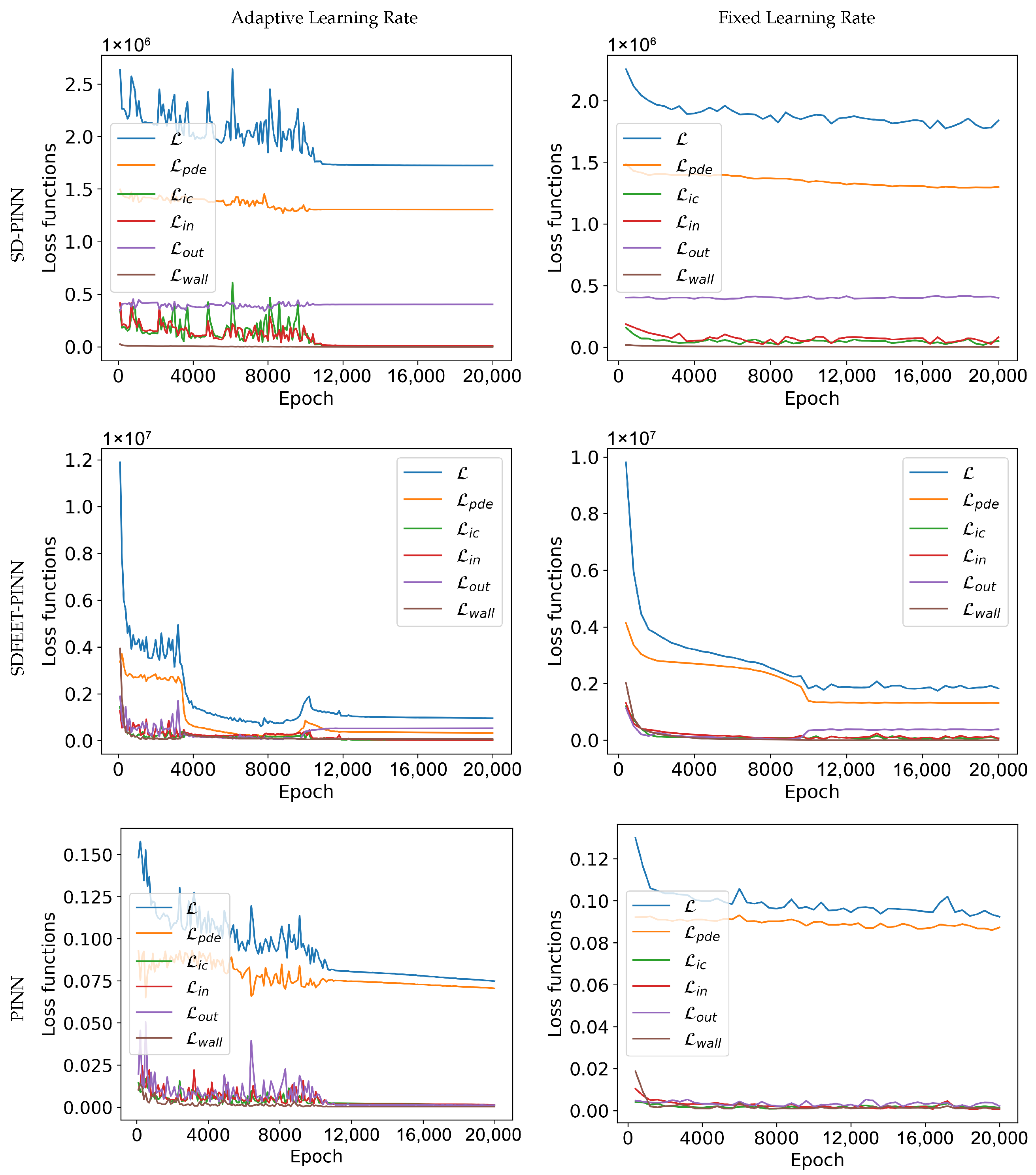
As shown in Figure 11, with SD-PINN using a Fixed Learning Rate (FLR), the global loss function, which is dominated by the outlet loss, quickly reaches a plateau. Even with the Adaptive Learning Rate (ALR), the outlet loss function only drops significantly after 4000 epochs. A similar sharp drop is observed for the classical PINN2 method at 2000 epochs, both for ALR and FLR.
For the classical PINN1 method, we observe significant oscillations with very large amplitudes, comparable to the magnitude of the sudden drops seen in other methods. All these aspects indicate substantial convergence difficulties.
In contrast, with the proposed SDFEET-PINN method, neither abrupt drops nor large oscillations are observed, except for a few moderate fluctuations. This behavior is expected, as the SDFEET-PINN approach tends to increase the equation residuals before gradually reducing them.
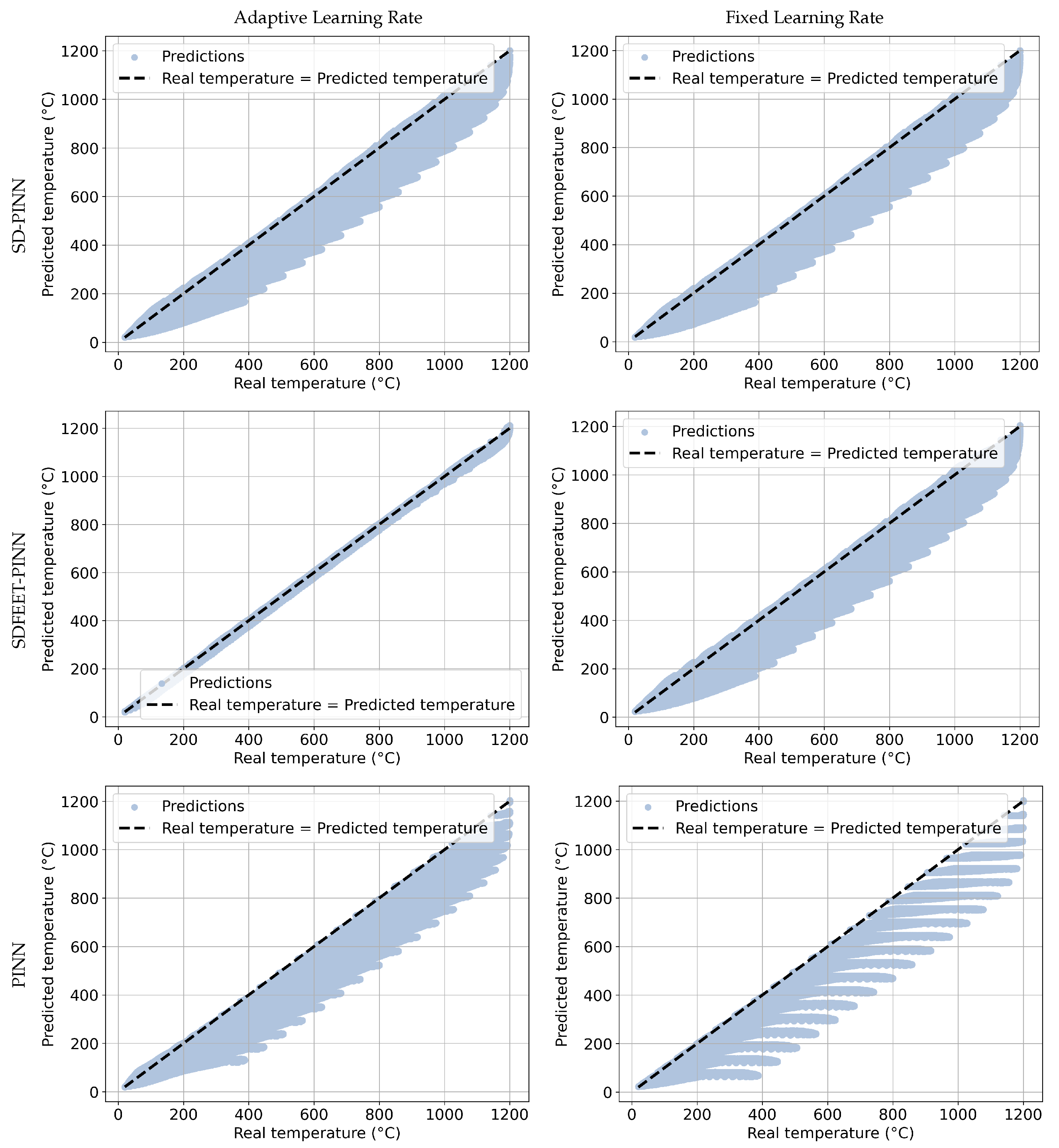
In the dispersion error graphs shown in Figure 12, for the SD-PINN method with FLR, horizontal points can be observed at the upper extremity of the predictions, confirming the convergence difficulties previously indicated by the plateau in Figure 11. However, with ALR, the predictions are significantly improved.
Once again, PINN2 produces poorer results with both ALR and FLR compared to PINN1, highlighting the considerable influence of the choice of normalization divisor in the classical method. The proposed SDFEET-PINN method delivers accurate predictions, similar to those obtained with the PINN1 method.
When examining the predicted temperature fields of ALR models in Figure 13, all methods appear to produce results consistent with the finite element simulation. The final frame clearly shows that the target temperature of 20   ° C at the inlet boundary is successfully achieved. Additionally, the Newton boundary condition applied at the outlet has generated a vertical red band of higher temperatures centered along the x-direction.
These visualizations alone do not allow for a clear comparison between the neural network models. To address this, the absolute error of the temperature field is analyzed in Figure 14, which clearly demonstrates that our two proposed methods, SD-PINN and SDFEET-PINN, outperform the others. However, the plot of the maximum error across all frames in Figure 15 indicates slightly better results for PINN1. In fact, the SD-PINN method with FLR and PINN2 are excluded from the comparison due to their poor performance, particularly PINN2, which exhibits significantly worse results.
All curves increase over time. One might suspect an error that could amplify over time, but this is not the case. Instead, it results from the fact that the Dirichlet boundary conditions and initial conditions are easier for the network to learn compared to the Newton boundary conditions, which are significantly more complex. In the early stages of the simulation, the influence of the boundary conditions is weaker compared to the initial condition. Additionally, in the final frames, the temperature field becomes more complex.
From the two problems with different boundary conditions, SDFEET-PINN performs best, followed by SD-PINN and PINN1. PINN2 is far behind the other three models. Since PINN1 is based on dividing the physical equation by C tran , and C tran is greater than C cond in both problems, we can consider PINN1 as a method that normalizes the physical equation by dividing it by the maximum value of its dimensional coefficients. Thus, adopting a normalization strategy using the maximum coefficient value as the divisor allows us to use only PINN1, avoiding the need to manage three classical methods. This is especially useful for the next problem, which will include three terms in the physical equation. In fact, an advection term will be added to the heat equation to test the robustness of the different methods. Hereafter, PINN1 will simply be referred to as PINN.

4.3. Problem with Advection, Dirichlet, and Newton Boundary Conditions

As shown in all graphs of Figure 16, the loss functions are dominated by the physical equation loss throughout all epochs, except for the graph of the SDFEET-PINN method with ALR, where, around epoch 12,000, the outlet loss function takes precedence.
As shown in Figure 17, the dispersion graphs clearly indicate that the SDFEET-PINN method with ALR provides better predictions than all other methods. In Figure 18, when observing the temperature field for models with ALR at the initial, intermediate, and final frames, the performance of the SDFEET-PINN method with the ALR model is clearly confirmed. This method is the only one where the physical equation loss function is not the most dominant. This suggests that the heat equation poses convergence difficulties in other methods. To investigate further, we evaluated the physical equation loss function in detail for all three methods with ALR.
Figure 19 shows that, in all methods, the final value of the conduction term becomes negligible compared to the other terms. The SDFEET-PINN method, due to its technique of increasing weaker terms to match the higher-value terms, initially had very high conduction and transient terms at the beginning of the epochs, allowing it to start from elevated values and descend toward equilibrium. It is observed that the convection term evolves less because it has the largest coefficient, and it is already at its true value from the start. The same evolution of terms is seen in the SDFEET-PINN method with FLR, but since the Learning Rate is fixed ( L R = 1   ×   10 4 ) and low at the beginning of the epochs, the curve is slower. Furthermore, the convection term does not coincide with the transient term until the end of the FEET strategy (around epoch 10,000), as seen in the SDFEET-PINN method with ALR. This coincidence appears to be the key difference between the two methods, as once the convection and transient terms coincide in the SDFEET-PINN method with ALR, this state remains stable until the end of the epochs, despite the variation in the values of the two terms. Additionally, in the SDFEET-PINN method with ALR, the conduction term rises after the FEET strategy finishes, reaching its true value, while this increase is not seen in the SDFEET-PINN method with FLR. It seems that this non-coincidence compensates for the lack of increase, as the displacement between the convection and transient terms in the SDFEET-PINN method with FLR appears to match the rise in the conduction term in the SDFEET-PINN method with ALR.
Given the convergence difficulties encountered with several methods, training was extended to 100,000 epochs for approaches using Adaptive Learning Rates (ALRs), and to 200,000 epochs for those with Fixed Learning Rates (FLRs). Additionally, the MSE loss function was used for FLR methods. The standard PINN method, which normalizes by the maximum coefficient, consistently failed to converge. As a result, we also evaluated the PINN1 variant, which normalizes the equation by the transient term coefficient and has shown better performance in previous problems. Training durations were approximately 4 h for 100,000 epochs and 8 h for 200,000 epochs. To focus the comparison on the final predicted temperature fields, Figure 20 presents the last frame of the simulations for various hyperparameter settings. The PINN method did not produce acceptable results in any configuration. PINN1 yielded improved predictions when MSE was used, but remained less accurate than our proposed SD-PINN. The latter provided sharper and more accurate temperature fields, including under ALR with 100,000 epochs. Moreover, the SDFEET-PINN approach demonstrated the best robustness, producing consistent results across all configurations starting from 100,000 epochs, and even from 20,000 epochs under ALR. The only failure case was under 20,000 epochs with MSE, where SD-PINN and, to a lesser extent, PINN1 still performed acceptably. These observations underscore the effectiveness of our proposed approaches across various training settings and highlight the critical influence of the normalization strategy in standard PINNs.

4.4. Application to a Complex 3D Geometry

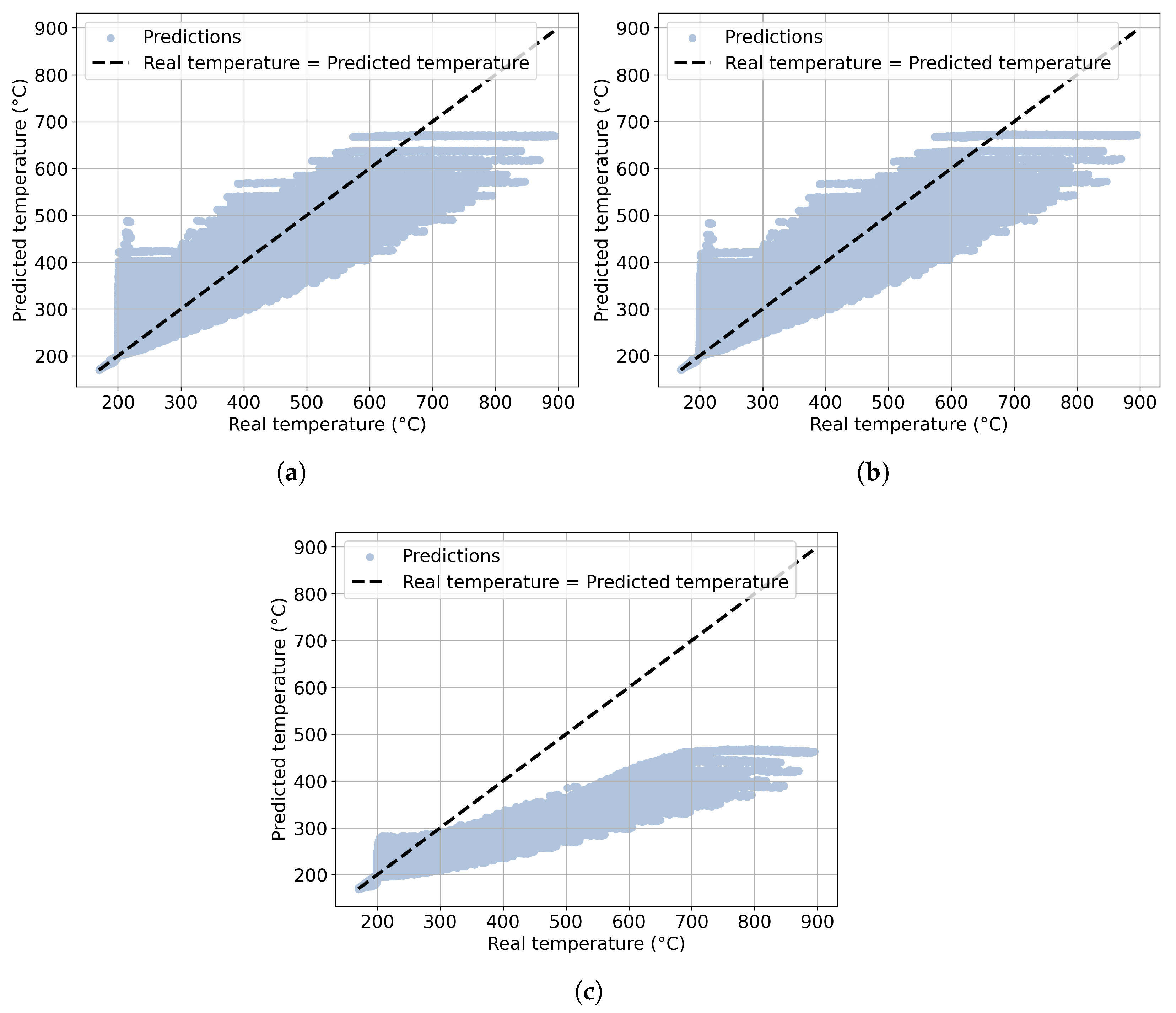
The dispersion curves of the results, shown in Figure 21, reveal poor predictions from all three models, with the classical PINN method yielding results worse than the SD-PINN and SDFEET-PINN methods. This is further confirmed by the temperature field results shown in Figure 22. The numerical model shows peak temperatures up to 896   ° C , while the proposed methods reach approximately 730 °C. Although this underestimation indicates that further refinement is needed, both SD-PINN and SDFEET-PINN clearly outperform the classical PINN approach, which only predicts about 400 °C and therefore fails to identify hot-spot regions in the part.
In this subsection, we can conclude that our two new methods yield promising results, especially considering this is the first attempt to address this problem with such a complex geometry. Indeed, the part is meshed using voxel elements, resulting in highly discontinuous surfaces. Moreover, the area that is less well predicted by our models compared to the numerical model consists of elements where many of them have their tops exposed to the boundary condition on the top surface of the part, while their bottoms and sides are exposed to the powder boundary condition. This results in multiple boundary conditions being imposed on the same element faces, with significant differences in their values. To improve accuracy, a higher number of collocation points will be required in these elements, or a more continuous mesh could be used. However, for additive manufacturing, we prefer voxel meshes due to their ease of use in various contexts. Therefore, in the future, we would stick with voxel elements, using many collocation points within these types of elements and prioritizing these collocation points, as some authors have implemented in the literature [17,25]. Our methods also have the advantage of being easily combined with other methods.

5. Conclusions

In this study, we introduced two novel weighting strategies for Physics-Informed Neural Networks (PINNs): the Same Dimensions PINN (SD-PINN) and the Same Dimensions From Equal Equation Terms PINN (SDFEET-PINN), and compared them with the classical PINN approach. The SD-PINN method balances the loss function terms by aligning their order of magnitude and physical dimensions. The SDFEET-PINN method pre-trains the network on a rebalanced governing equation and, after an initial stabilization of the learning process, progressively restores the original formulation, thereby preserving the influence of all terms across different orders of magnitude. After demonstrating that the hyperbolic tangent (tanh) function is the most suitable activation function, we introduced a new Adaptive Learning Rate (ALR) method, which significantly improved the quality of the results. Through the analysis of convergence graphs, dispersion plots, and temperature fields, we gained valuable insights into the convergence issues encountered by the methods and demonstrated how our approach enhances PINN convergence. The SDFEET-PINN method, combined with ALR, proved to be highly effective, converging to the solution for all the tested cases. The second-best performing method was SD-PINN with ALR, followed by the classical PINN method with ALR, also with ALR. Furthermore, we highlighted the importance of selecting the correct divisor for the normalization of the physical equation in the classical PINN method. It should be emphasized that, although the underlying heat transfer equation is physically simple, the combined presence of multiple boundary condition types and complex 3D voxel geometries makes these problems particularly demanding for PINNs. The proposed SD-PINN and SDFEET-PINN methods demonstrate their ability to handle such configurations with improved stability and accuracy compared to classical approaches.
In conclusion, SDFEET-PINN clearly offers a robust and efficient alternative to classical PINNs for addressing complex thermal problems. Its superior convergence behavior and accuracy make it a promising tool for advanced simulations involving varying boundary conditions and complex flow dynamics. Additionally, this method is advantageous because it can be applied to a wide range of existing techniques in the literature, as it focuses solely on the normalization of equations.
Looking forward, this study should be further explored by testing additional hyperparameters, including optimizers, different network dimensions, and even other physical models, such as the Navier–Stokes equations, in order to generalize the approach. Regarding the methods themselves, certain arbitrary choices, such as the use of a coefficient of 0.01 to represent 1% of the residual error terms, and the relationship between the spatiotemporal size of the model and its spatiotemporal increments, Δ t and Δ l , require further investigation. A future objective will be to systematically explore whether alternative combinations of these parameters could further improve convergence performance. Furthermore, future extensions to multiphysics problems will involve an even larger number of coefficients to normalize, highlighting the relevance of the methodological framework proposed in this study. Further work should also focus on benchmarking the proposed methods using adaptive and weak-form PINN strategies, in order to verify the generalization of the method to various PINN strategies.
The focus will also move to real-time simulations, accounting for the progressive construction of the part in additive manufacturing, a key step toward developing the process digital twin.

Author Contributions

Conceptualization, A.T.; methodology, A.T.; software, A.T.; validation, A.T. and L.A.; formal analysis, A.T. and L.A.; investigation, A.T.; resources, A.T.; data curation, A.T. and L.A.; writing—original draft preparation, A.T.; writing—review and editing, A.T. and L.A.; visualization, A.T. and L.A.; supervision, A.T.; project administration, A.T. All authors have read and agreed to the published version of the manuscript.

Funding

This research received no external funding.

Data Availability Statement

The original data presented in the study are openly available in https://zenodo.org/account/settings/github/repository/tongne/Physics-Informed-Neural-Networks-SD-PINN-SDFEET-PINN (accessed on 6 November 2025).

Conflicts of Interest

The authors declare no conflicts of interest.

Nomenclature

Abbreviations
AbbreviationDescription
L-PBFLaser Powder Bed Fusion
PINNPhysics-Informed Neural Networks
FEMFinite Element Method
FVMFinite Volume Method
FDMFinite Difference Method
SD-PINNSame Dimensions PINN
PDEPartial Differential Equation, specifically the heat equation.
ADAMAdaptive Moment Estimation.
L-BFGSLimited-memory Broyden–Fletcher–Goldfarb–Shanno.
SDFEET-PINNSame Dimensions From Equal Equation Terms PINN
FEETFrom Equal Equation Terms PINN
Symbols
SymbolDescription
lThe width of the model geometry.
L 0 The length of the model geometry, also used as the reference length.
f ( x , y ) Prescribed initial temperature function.
g ( x , y ) Prescribed temperature or flux, depending on the operator B .
ρ Density.
cSpecific heat.
λ Heat conductivity.
B Boundary condition operator
[ ] * Exponent * denotes the dimensionless variables.
[ ] 0 Subscript 0 denotes the reference constants.
R i Residual related to i ∈ {pde, ic, in, out, wall, bot, pow, top}.
L i Loss related to i ∈ {pde, ic, in, out, wall, bot, pow, top}.
C i Dimensional coefficients related to i ∈ {tran, conv, cond, ic, in, out, out/h, out/k, bot, pow/h, pow/k, top/p, top/h}.
[ ] tran Subscript indicating variables related to the transient term in the heat equation.
[ ] conv Subscript indicating variables related to the convection term in the heat equation.
[ ] cond Subscript indicating variables related to the conduction term in the heat equation.
[ ] pde Subscript indicating variables related to the Partial Differential Equation or the heat equation.
[ ] ic Subscript indicating variables related to the initial conditions.
[ ] in Subscript indicating variables related to the inlet boundary condition.
[ ] out Subscript indicating variables related to the outlet boundary condition.
[ ] out / h and [ ] out / k Subscripts of the coefficients for the convection and conduction terms in the Newton boundary condition at the outlet, respectively.
[ ] wall Subscript indicating variables related to the wall boundary condition.
[ ] bot Subscript indicating variables related to the bottom boundary condition.
[ ] pow / h , and [ ] pow / k Subscripts of the coefficients for the convection and conduction terms in the Newton boundary condition at the surface in contact with the powder, respectively.
[ ] top / p , [ ] top / h and [ ] top / k Subscripts of the coefficients for the prescribed heat flux power, convection, and conduction terms in the Newton boundary condition at the top surface of the 3D hydraulic joint, respectively.

References

  1. Gao, S.; Li, Z.; Petegem, S.V.; Ge, J.; Goel, S.; Vas, J.V.; Luzin, V.; Hu, Z.; Seet, H.L.; Sanchez, D.F.; et al. Additive manufacturing of alloys with programmable microstructure and properties. Nat. Commun. 2023, 14, 6752. [Google Scholar] [CrossRef]
  2. Bajaj, P.; Hariharan, A.; Kini, A.; Kürnsteiner, P.; Raabe, D.; Jägle, E.A. Steels in additive manufacturing: A review of their microstructure and properties. Mater. Sci. Eng. A 2020, 772, 138633. [Google Scholar] [CrossRef]
  3. Delahaye, J.; Tchuindjang, J.T.; Lecomte-Beckers, J.; Rigo, O.; Habraken, A.M.; Mertens, A. Influence of Si precipitates on fracture mechanisms of AlSi10Mg parts processed by Selective Laser Melting. Acta Mater. 2019, 175, 160–170. [Google Scholar] [CrossRef]
  4. Pauza, J.G.; Tayon, W.A.; Rollett, A.D. Computer simulation of microstructure development in powder-bed additive manufacturing with crystallographic texture. Model. Simul. Mater. Sci. Eng. 2021, 29, 055019. [Google Scholar] [CrossRef]
  5. Khdoudi, A.; Masrour, T.; Hassani, I.E.; Mazgualdi, C.E. A Deep-Reinforcement-Learning-Based Digital Twin for Manufacturing Process Optimization. Systems 2024, 12, 38. [Google Scholar] [CrossRef]
  6. Zhu, Q.; Liu, Z.; Yan, J. Machine learning for metal additive manufacturing: Predicting temperature and melt pool fluid dynamics using physics-informed neural networks. Comput. Mech. 2021, 67, 619–635. [Google Scholar] [CrossRef]
  7. Nath, P.; Mahadevan, S. Probabilistic Digital Twin for Additive Manufacturing Process Design and Control. J. Mech. Des. 2022, 144, 1–15. [Google Scholar] [CrossRef]
  8. Go, M.S.; Lim, J.H.; Lee, S. Physics-informed neural network-based surrogate model for a virtual thermal sensor with real-time simulation. Int. J. Heat Mass Transf. 2023, 214, 124392. [Google Scholar] [CrossRef]
  9. Zhou, G.; Zhang, C.; Li, Z.; Ding, K.; Wang, C. Knowledge-driven digital twin manufacturing cell towards intelligent manufacturing. Int. J. Prod. Res. 2020, 58, 1034–1051. [Google Scholar] [CrossRef]
  10. Bresson, Y.; Tongne, A.; Baili, M.; Arnaud, L. Global-to-local simulation of the thermal history in the laser powder bed fusion process based on a multiscale finite element approach. Int. J. Adv. Manuf. Technol. 2023, 127, 4727–4744. [Google Scholar] [CrossRef]
  11. De Lozzo, M. Substitution de modèle et approche multifidélité en expérimentation numérique [Surrogate modeling and multifidelity approach in computer experimentation]. J. Société Française Stat. 2015, 156, 21–55. [Google Scholar]
  12. Aymerich, E.; Pisano, F.; Cannas, B.; Sias, G.; Fanni, A.; Gao, Y.; Böckenhoff, D.; Jakubowski, M. Physics Informed Neural Networks towards the real-time calculation of heat fluxes at W7-X. Nucl. Mater. Energy 2023, 34, 101401. [Google Scholar] [CrossRef]
  13. Raissi, M.; Perdikaris, P.; Karniadakis, G. Physics-informed neural networks: A deep learning framework for solving forward and inverse problems involving nonlinear partial differential equations. J. Comput. Phys. 2019, 378, 686–707. [Google Scholar] [CrossRef]
  14. Xu, R.; Zhang, D.; Rong, M.; Wang, N. Weak form theory-guided neural network (TgNN-wf) for deep learning of subsurface single- and two-phase flow. J. Comput. Phys. 2021, 436, 110318. [Google Scholar] [CrossRef]
  15. Rong, M.; Zhang, D.; Wang, N. A Lagrangian dual-based theory-guided deep neural network. Complex Intell. Syst. 2022, 8, 4849–4862. [Google Scholar] [CrossRef]
  16. Zhou, H.; Wu, H.; Sheil, B.; Wang, Z. A self-adaptive physics-informed neural networks method for large strain consolidation analysis. Comput. Geotech. 2025, 181, 107131. [Google Scholar] [CrossRef]
  17. Hou, J.; Li, Y.; Ying, S. Enhancing PINNs for solving PDEs via adaptive collocation point movement and adaptive loss weighting. Nonlinear Dyn. 2023, 111, 15233–15261. [Google Scholar] [CrossRef]
  18. Guo, Y.; Cao, X.; Song, J.; Leng, H.; Peng, K. An efficient framework for solving forward and inverse problems of nonlinear Partial Differential Equations via enhanced physics-informed neural network based on adaptive learning. Phys. Fluids 2023, 35, 106603. [Google Scholar] [CrossRef]
  19. Xiang, Z.; Peng, W.; Liu, X.; Yao, W. Self-adaptive loss balanced Physics-informed neural networks. Neurocomputing 2022, 496, 11–34. [Google Scholar] [CrossRef]
  20. Wang, J.; Xiao, X.; Feng, X.; Xu, H. An improved physics-informed neural network with adaptive weighting and mixed differentiation for solving the incompressible Navier–Stokes equations. Nonlinear Dyn. 2024, 112, 16113–16134. [Google Scholar] [CrossRef]
  21. Gao, B.; Yao, R.; Li, Y. Physics-informed neural networks with adaptive loss weighting algorithm for solving partial differential equations. Comput. Math. Appl. 2025, 181, 216–227. [Google Scholar] [CrossRef]
  22. Hooshyar, S.; Elahi, A. Sequencing Initial Conditions in Physics-Informed Neural Networks. J. Chem. Environ. 2024, 3, 98–108. [Google Scholar] [CrossRef]
  23. Chen, X.; Yang, J.; Liu, X.; He, Y.; Luo, Q.; Chen, M.; Hu, W. Hemodynamics modeling with physics-informed neural networks: A progressive boundary complexity approach. Comput. Methods Appl. Mech. Eng. 2025, 438, 117851. [Google Scholar] [CrossRef]
  24. Guo, Y.; Min, J.; Lin, S.; Liu, X.; Fu, Z. Curriculum-Transfer-Learning Based Physics-Informed Neural Networks for Long-Term Simulation of Physical and Mechanical Behaviors. Chin. J. Theor. Appl. Mech. 2024, 56, 763–773. [Google Scholar] [CrossRef]
  25. Münzer, M.; Bard, C. A Curriculum-Training-Based Strategy for Distributing Collocation Points during Physics-Informed Neural Network Training. In Proceedings of the Machine Learning and the Physical Sciences Workshop, New Orleans, LA, USA, 3 December 2022. [Google Scholar]
  26. Peng, B.; Panesar, A. Multi-layer thermal simulation using physics-informed neural network. Addit. Manuf. 2024, 95, 104498. [Google Scholar] [CrossRef]
  27. Ghungrad, S.; Gould, B.; Wolff, S.; Haghighi, A. Physics-Informed Artificial Intelligence for Temperature Prediction in Metal Additive Manufacturing: A Comparative Study. In Volume 1: Additive Manufacturing Biomanufacturing; Life Cycle Engineering; Manufacturing Equipment and Automation; Nano/Micro/Meso Manufacturing; American Society of Mechanical Engineers: New York, NY, USA, 2022. [Google Scholar] [CrossRef]
  28. Huang, Y.H.; Xu, Z.; Qian, C.; Liu, L. Solving free-surface problems for non-shallow water using boundary and initial conditions-free physics-informed neural network (bif-PINN). J. Comput. Phys. 2023, 479, 112003. [Google Scholar] [CrossRef]
  29. Kashefi, A.; Mukerji, T. Physics-informed PointNet: A deep learning solver for steady-state incompressible flows and thermal fields on multiple sets of irregular geometries. J. Comput. Phys. 2022, 468, 111510. [Google Scholar] [CrossRef]
  30. Bolandi, H.; Sreekumar, G.; Li, X.; Lajnef, N.; Boddeti, V.N. Physics informed neural network for dynamic stress prediction. Appl. Intell. 2023, 53, 26313–26328. [Google Scholar] [CrossRef]
  31. Bresson, Y.; Tongne, A.; Selva, P.; Arnaud, L. Numerical modelling of parts distortion and beam supports breakage during selective laser melting (SLM) additive manufacturing. Int. J. Adv. Manuf. Technol. 2022, 119, 5727–5742. [Google Scholar] [CrossRef]
  32. Benoist, V.; Arnaud, L.; Baili, M.; Faye, P. Topological optimization design for additive manufacturing, taking into account flexion and vibrations during machining post processing operations. In Proceedings of the 14th International Conference on High Speed Machining, San Sebastián, Spain, 17–18 April 2018; pp. 1–4. [Google Scholar]
  33. Lou, Q.; Meng, X.; Karniadakis, G.E. Physics-informed neural networks for solving forward and inverse flow problems via the Boltzmann-BGK formulation. J. Comput. Phys. 2021, 447, 110676. [Google Scholar] [CrossRef]
  34. Pratama, D.A.; Abo-Alsabeh, R.R.; Bakar, M.A.; Salhi, A.; Ibrahim, N.F. Solving partial differential equations with hybridized physic-informed neural network and optimization approach: Incorporating genetic algorithms and L-BFGS for improved accuracy. Alex. Eng. J. 2023, 77, 205–226. [Google Scholar] [CrossRef]
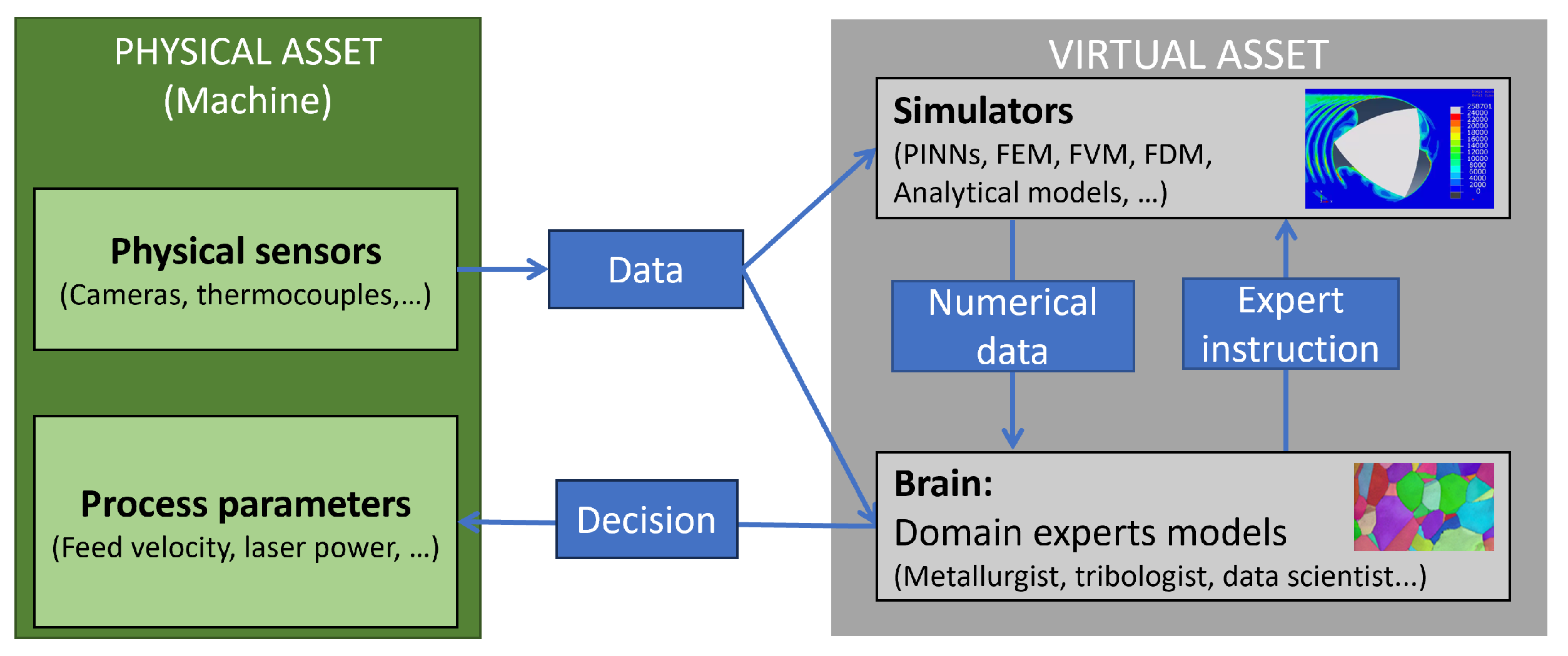
Figure 1. Illustration of the digital twin of manufacturing processes.
Applsci 15 12234 g001
Figure 2. Geometry of the model.
Applsci 15 12234 g002
Figure 3. Architecture of classical PINN.
Applsci 15 12234 g003
Figure 4. Weighting coefficients. (a) SD-PINN; (b) SDFEET-PINN.
Applsci 15 12234 g004
Figure 5. Velocity field profile in the domain.
Applsci 15 12234 g005
Figure 6. Voxel mesh of the hydraulic joint with top and bottom boundary conditions.
Applsci 15 12234 g006
Figure 7. Loss functions of the Dirichlet boundary conditions problem.
Applsci 15 12234 g007
Figure 8. Dispersion graphs of the Dirichlet boundary conditions problem.
Applsci 15 12234 g008
Figure 9. Comparison of the predicted temperature field ( ° C ) with that of the finite element model for the Dirichlet boundary conditions problem.
Applsci 15 12234 g009
Figure 10. Field of absolute temperature error ( ° C ) for the Dirichlet boundary conditions problem.
Applsci 15 12234 g010
Figure 11. Loss functions of the Dirichlet and Newton boundary conditions problem.
Applsci 15 12234 g011
Figure 12. Dispersion graphs of the Dirichlet and Newton boundary conditions problem.
Applsci 15 12234 g012
Figure 13. Comparison of the predicted temperature field ( ° C ) with that of the finite element model for the Dirichlet and Newton boundary conditions problem.
Applsci 15 12234 g013
Figure 14. Field of absolute temperature error ( ° C ) for the Dirichlet and Newton boundary conditions problem.
Applsci 15 12234 g014
Figure 15. Maximum absolute error of the temperature field predicted by the SD-PINN method with ALR, SDFEET-PINN, and PINN1.
Applsci 15 12234 g015
Figure 16. Loss functions of the Advection problem.
Applsci 15 12234 g016
Figure 17. Dispersion graphs of the Advection problem.
Applsci 15 12234 g017
Figure 18. Comparison of the temperature field ( ° C ) predicted by SD-PINN, SDFEET-PINN, and classical PINN for the Advection problem.
Applsci 15 12234 g018
Figure 19. Graphs of the terms in the heat equation for the Advection problem.
Applsci 15 12234 g019
Figure 20. Temperature fields predicted under various hyperparameter settings, including different training epochs, error metrics (Root Mean Square Error and Mean Square Error), and learning rate strategies (adaptive and fixed).
Applsci 15 12234 g020
Figure 21. Dispersion graphs of the complex geometry problem. (a) SD-PINN; (b) SDFEET-PINN; (c) PINN.
Applsci 15 12234 g021
Figure 22. Comparison of the predicted temperature field ( ° C ) from SD-PINN, SDFEET-PINN, and PINN, with the finite element model results.
Applsci 15 12234 g022
Disclaimer/Publisher’s Note: The statements, opinions and data contained in all publications are solely those of the individual author(s) and contributor(s) and not of MDPI and/or the editor(s). MDPI and/or the editor(s) disclaim responsibility for any injury to people or property resulting from any ideas, methods, instructions or products referred to in the content.