Article

A Shallow Foundation Settlement Prediction Method Considering Uncertainty Based on Machine Learning and CPT Data

1
School of Civil Engineering and Water Resources, Qinghai University, Xining 810016, China
2
Key Laboratory of Energy-Saving Building Materials and Engineering Safety, Xining 810016, China
*
Author to whom correspondence should be addressed.
Appl. Sci. 2025, 15(22), 12174; https://doi.org/10.3390/app152212174
Submission received: 13 October 2025 / Revised: 14 November 2025 / Accepted: 15 November 2025 / Published: 17 November 2025

Abstract

In the field of geoengineering, predicting foundation settlement is a critical topic. Traditional settlement prediction methods struggle to accurately reflect settlement under complex geological conditions. This study combines cone penetration test (CPT) data and collects data from 46 different geoengineering sites from the literature. Gradient Boosting Decision Tree (GBDT), Extreme Gradient Boosting (XGBoost), Deep Neural Network (DNN), Support Vector Machine (SVM), and Random Forest (RF) models are individually established, and an ensemble model is proposed to predict shallow foundation settlement St. The results show that the proposed ensemble model exhibits the best predictive performance, providing a reference for practical engineering projects. The predictions of the optimal model are compared with those of single models and traditional methods, and the uncertainty of model predictions is quantified using Monte Carlo Simulation (MCS). Sensitivity analyses are conducted using feature importance analysis and SHAP methods to assess the influence of input parameters on the prediction results. Finally, Generative Adversarial Networks (GANs) are introduced to generate new data to validate the generalization capability of the model.

1. Introduction

The prediction of settlement for shallow foundations is directly related to the safety and service life of buildings and is crucial in the field of civil engineering. The vast majority of structures are supported by shallow foundations, and settlement is the primary controlling factor considered in the design of shallow foundations [1]. Settlement of shallow foundations can lead to cracks, tilting, deformation, and even structural failure of buildings, severely affecting their functionality and safety. With the acceleration of urbanization, the number and scale of buildings continue to increase, raising higher demands on foundation engineering. Especially in soft soil regions, settlement problems are more pronounced due to the high compressibility and low bearing capacity of the foundation soil layers. Therefore, accurate settlement analysis and estimation are important topics in the design of shallow foundations.
Traditional settlement prediction methods are heavily data-dependent, requiring a large amount of field test data, which is time-consuming, labor-intensive, and costly to obtain. Due to the complexity and variability of geological conditions, there remain many uncertainties in geotechnical engineering [2], posing significant challenges to the practical application of traditional settlement prediction methods. These methods struggle to accurately reflect settlement behavior, thus impacting the reliability of engineering design and construction. Therefore, accurately predicting the settlement of shallow foundations remains a challenging task.
In shallow foundation design, the fundamental equation for calculating foundation settlement is based on soil stiffness (E), foundation width (B), contact stress (q), and the stress distribution with depth. These parameters are influenced by soil type, time, and loading conditions. Using a single soil property value as the average stiffness of all soil layers can lead to bias in settlement estimation [3]. By improving the quality and quantity of field investigation tests, the uncertainty in foundation settlement analysis can be reduced. With the rapid development of in situ testing technologies, they have played an important role in geotechnical engineering design [4,5]. Among these, CPT (Cone Penetration Testing) has become a crucial tool for characterizing foundation soil layers due to its high resolution and accuracy [6]. CPT data can provide information about soil stratigraphy, density, and strength, which is vital for accurately predicting foundation settlement [7,8]. However, accurately and effectively integrating CPT data with machine learning models and quantifying the uncertainty of predictions remains a topic worthy of further research [9].
In recent years, with the development of machine learning techniques, an increasing number of researchers have attempted to apply them to settlement prediction to improve accuracy and reliability. Methods such as Gradient Boosting Decision Tree (GBDT), Extreme Gradient Boosting (XGBoost), Support Vector Machine (SVM), Artificial Neural Network (ANN), and Decision Tree (DT) have been widely applied in the field of civil engineering [10,11], for example, in intelligent seismic risk assessment [12], intelligent prediction of tunnel deterioration [13], and geological layer classification [14].
Among them, GBDT is an ensemble learning method that builds multiple decision trees sequentially, with each tree learning the residuals of the preceding trees [15]. XGBoost is an efficient implementation of GBDT that optimizes speed and performance using techniques such as second-order Taylor expansion, regularization terms, and parallel processing [16]. Deep neural networks (DNNs) are a type of artificial neural network architecture that extract and combine features of input data layer by layer through multiple layers of neurons, enabling automatic modeling and prediction of complex nonlinear relationships [17]. Support vector machines (SVMs) are a commonly used supervised learning method suitable for handling high-dimensional data and complex boundary problems [18], using nonlinear kernel functions to capture the complex relationships between input parameters and settlement. Random forest (RF) is a decision tree–based ensemble learning method with strong feature selection capability and resistance to overfitting [19]. By aggregating multiple decision trees, random forest can effectively improve model stability and predictive accuracy [20]. However, single machine learning models may have certain limitations when handling complex problems. For example, SVMs can have high computational complexity when processing large-scale data [21], while random forest—despite its stability—may perform inadequately on time-series data. Therefore, combining the strengths of multiple models to develop hybrid algorithms may be an effective approach to addressing settlement prediction problems [18,22].
This paper proposes a shallow foundation settlement prediction method based on machine learning and CPT data. Forty-six datasets from different geological conditions were collected from the literature. GBDT, XGBoost, DNN, SVM, and RF models were developed, and an ensemble model was proposed. Multiple model architectures were systematically compared using 5-fold nested cross-validation to determine the “best” ensemble; exhaustive grid searches were used for hyperparameter tuning, and the nested cross-validation employed outer folds for performance assessment and inner folds for parameter tuning to eliminate bias [23]. A small independent test set was reserved, reflecting the limited validation-data scenarios encountered in engineering practice. The test set was completely independent of the training process and provided a true external validation of performance. Comparing the predictive accuracy of each model showed that the SVM-ensemble RF model outperformed the other models. To validate the effectiveness of the proposed ensemble, the SVM-ensemble RF model’s predictions were compared with those from traditional settlement prediction methods, and Monte Carlo simulation (MCS) was used to quantify uncertainty in the ensemble model’s predictions [24,25]. Results indicate that the SVM-ensemble RF model surpasses the other models and traditional methods in both predictive accuracy and stability. In addition, to further analyze the influence of input parameters on predictions, feature importance and SHAP (Shapley Additive Explanations) values were used to conduct a sensitivity analysis of the model [26,27]. This revealed the contribution of each input parameter to settlement prediction and provided guidance for parameter selection and optimization in engineering practice. Finally, to verify the model’s generalization capability, 50 new datasets were generated using generative adversarial networks (GANs) based on the 46 datasets collected from the literature and used with the proposed ensemble model.
With the continuous advancement of data acquisition technologies and the ongoing development of machine learning algorithms, future research can further explore how to integrate more types of data (such as remote sensing data, seismic data, etc.) with machine learning models to improve the accuracy and applicability of settlement prediction [28,29,30]. Additionally, incorporating uncertainty analysis and risk assessment into the models is also a worthwhile direction for in-depth study. Through the research presented in this paper, we hope to provide a machine learning-based settlement prediction method for shallow foundations that is more accurate and widely applicable, thereby promoting technological progress and application development in this field.

2. Traditional Method

A significant amount of research has been conducted on predicting shallow foundation settlement using empirical correlations based on CPT records. These relationships primarily consider the soil’s elastic modulus ( E s ), foundation width (B), contact pressure (q), and cone tip resistance ( q c ). A summary of the most common analytical methods reported in the literature is presented in Table 1. From Table 1, it can be seen that Janbu (1967) [31], Schmerthmann (1978) [32], and Berardi and Lancellotta (1991) [33] provided a fundamental formula for calculating settlement values based on static cone penetration test results. Recently, Malekdoost and Eslami (2011) [34] and Valikhah and Eslami (2019) [3] modified Janbu’s equation by adding several other terms to the modulus (m). It is worth noting that the accuracy of the formulas provided in Table 1 is relatively high when approaching the ultimate bearing capacity or within the range of S t /B = 0.1 [35]. All relationships in Table 1 were obtained from various case studies through plate load tests (PLT). Based on PLT results, weightings that lead to plate failure can be determined. Conversely, allowable bearing capacity of piles can be calculated by permitting a certain amount of settlement.
Although the recommended formulas in Table 1 vary due to factors such as soil type, time, and loading conditions, there is still a lack of a universal method capable of accurately predicting foundation settlement in geotechnical engineering practice. Predicting foundation settlement involves complex nonlinear characteristics and the coupled effects of multiple variables, making the development of a model that can capture the complexity of foundation soil layers and improve prediction accuracy highly significant.
To address the aforementioned issues, this study employs various machine learning models and ensemble models to predict shallow foundation settlement and compares the prediction results of each model. The proposed ensemble model, alongside single models and traditional methods, has been validated through Monte Carlo simulation uncertainty analysis, demonstrating its capability to accurately predict shallow foundation settlement with different geotechnical parameters under continuous CPT records.

3. Case Study Records

Table 2 provides an overview of a database containing 46 cases used for model development and analysis in this study. As shown in Table 2, the cases include 22 square, 17 circular, and 7 rectangular foundations. B represents the foundation width, D f the foundation depth, q the foundation load, q t the corrected q c , R f the friction ratio, and S t the settlement amount. The foundation embedment depth ranges from 0 to 2.35 m, with measured settlements in these cases ranging from 25 to 260 mm, where S t /B is approximately 2% to 10% of the foundation width. According to the soil and loading conditions mentioned in Schmertmann (1978) [32], the effective depth under the foundation is approximated as 2B. Table 2 considers the arithmetic averages of CPT-related parameters down to a depth of 2B beneath the foundation (i.e., R f and q t ). It is noteworthy that in all cases of the present study, loads are assumed to be located near St/B = 0.1, where St/B = 0.1 is the quality standard for sand PLT. Previous studies, including Malekdoost and Eslami (2011) [34] and Valikhah and Eslami (2019) [3], have detailed the validity of the current data referenced in this paper.
It is worth noting that the database can be expanded so that, at each stage of the loading test, the corresponding settlement for each load on the foundation can be regarded as part of the database, and in fact, more datasets can be envisioned. However, when the soil fails, the soil conditions beneath the footing will be similar to those recorded in the CPT data (such as q t ). Therefore, the load on the foundation corresponding to the CPT record is the ultimate load (q) [39]. This provides a theoretical basis for the input parameters of the model.
In this study, the soil St is considered to be influenced by the foundation width B, the corrected cone tip resistance q t , and the foundation load q. Although other parameters such as R f , I c , OCR, and D r may provide incremental improvements in specific geological settings, the current trio captures the fundamental mechanics of foundation settlement in cohesionless soils. The demonstrated performance indicates that this simplified approach offers a powerful practical tool for preliminary design and rapid assessment; therefore, B, q t , and q are used as input parameters for the SVM-integrated RF model. The relationship between these three input parameters and the output parameter is shown in Figure 1.

4. Modeling Process

4.1. Gradient Boosting Decision Tree (GBDT)

Gradient Boosting Decision Tree (GBDT) is an ensemble learning algorithm [15]. Its core idea is to iteratively train a new weak learner (usually a decision tree) each round to correct the residuals of the previous model, using gradient descent to minimize the loss function. Each round learns the negative gradient direction of the loss function, and the final prediction is obtained by weighted summation of all weak learners’ outputs. GBDT has the following characteristics: it can handle nonlinear relationships, is relatively robust to outliers, does not require feature standardization, and offers relatively good interpretability.

4.2. Extreme Gradient Boosting (XGBoost)

Extreme Gradient Boosting (XGBoost) is an efficient implementation of GBDT [16] and includes the following improvements: L1 and L2 regularization terms added to the objective function to effectively prevent overfitting; although boosting is a serial process, XGBoost can parallelize feature selection and split-finding; missing value handling: it automatically learns how to handle missing values; pruning strategy: uses post-pruning for greater precision; cache optimization: data structures and algorithms are optimized for faster training. XGBoost offers the following advantages: excellent performance, high computational efficiency, built-in cross-validation, and support for custom objective functions.

4.3. Deep Neural Network (DNN)

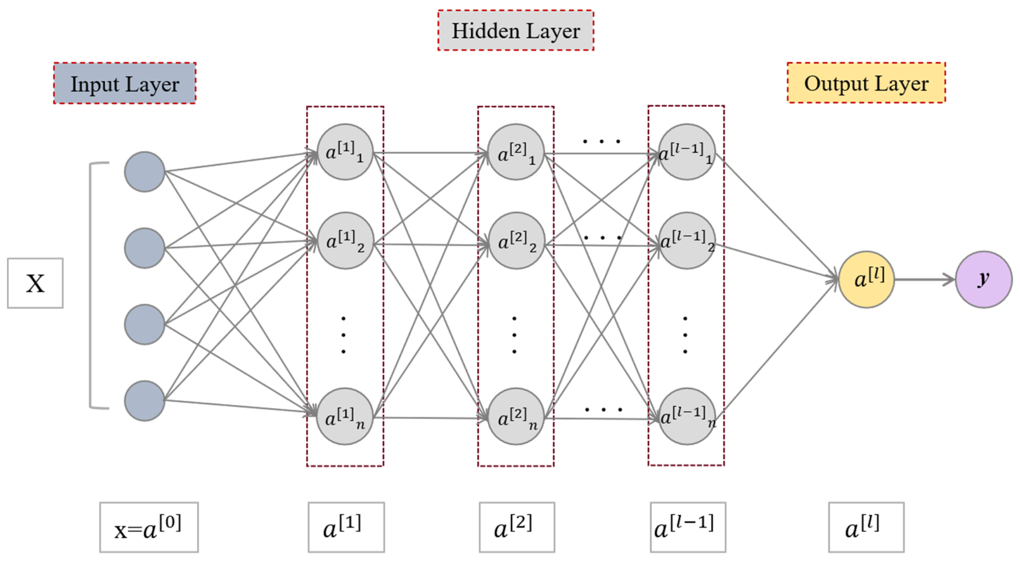
A Deep Neural Network (DNN) is a neural network model composed of multiple neurons and hidden layers, featuring a multilayer structure. It is a supervised learning model proficient in handling high-dimensional data and complex nonlinear problems. The core idea of a DNN is to automatically extract features and construct mapping relationships through data-driven methods. It is widely applied in tasks such as classification, regression, image recognition, and sequence prediction. The model structure is shown in Figure 2 [17].
Suppose there is a neural network with l-layers, where the computation of each layer’s neurons can be represented as:
z l = W l · a l 1 + b l
a l = f z l
y ^ = a l
where z l is the linear output of the l-th layer, W l is the weight matrix of the l-th layer, b l is the bias vector of the l-th layer, a l 1 is the nonlinear activation output of the (l-1)-th layer and y ^ is the predicted output of the neural network.
Use a loss function to measure the error between predicted values and true values.
L = 1 m i = 1 m y ^ i y i 2
where y ^ i is the predicted value of the i-th training sample, y i is the true value or label of the i-th training sample.
Use the Adam optimizer to update parameters based on gradients, minimizing the loss function through the optimization algorithm:
W l : = W l α L W l , b l : = b l α L b l
m t = β 1 m t 1 + 1 β 1 g t , v t = β 2 v t 1 + 1 β 2 g t 2
W : = W α m t v t + ϵ
where α is the learning rate, m t is the first-order momentum, and v t is the second-order momentum.

4.4. Support Vector Machines (SVM)

Support Vector Machine (SVM) is a supervised learning model used for classification and regression tasks. Its core idea is to find an optimal hyperplane in the feature space to effectively separate and predict data points. In classification tasks, SVM improves the model’s generalization ability by maximizing the margin of the decision boundary, while in regression tasks, SVM aims to find a function f(x) whose deviation from the actual target value y at each training point does not exceed ϵ , while keeping the function as flat as possible.
The goal of Support Vector Regression (SVR) is to achieve predictions by optimizing the following function [18]:
f x = ω , x + b
where ω , x represents the inner product of ω and x , x is the input feature vector, ω is the weight vector, which defines the normal vector to the hyperplane learned by the SVR model, and b is the bias term. To achieve this goal, SVR needs to solve the following optimization problem:
m i n 1 2 ω 2 + C i = 1 n ξ i + ξ i
where ‘min’ is the minimum value of the first item.
The constraints are:
y i ω , x i b ϵ + ξ i
ω , x i + b y i ϵ + ξ i
ξ i , ξ i 0
In this context, ξ i and ξ i * are slack variables used to handle deviations beyond ϵ , while C is the regularization parameter that controls the trade-off between the model’s tolerance for errors and its complexity.
To handle nonlinear data, the SVM model introduces a kernel function, which maps the original feature space to a higher-dimensional feature space, thereby finding a linear hyperplane in the high-dimensional space to solve the nonlinear problem.

4.5. Random Forest (RF)

Random Forest (RF) is an ensemble learning method widely used for classification and regression tasks. Its core idea is to improve the accuracy and stability of the model by constructing multiple decision trees and combining their prediction results. In regression tasks, Random Forest generates the final prediction value by averaging the predictions of all decision trees, effectively reducing the overfitting problem that may occur with individual decision trees. The prediction formula for the random forest is as follows [19]:
y ^ = 1 T t = 1 T h t x
In this context, T represents the number of decision trees, and h t x is the predicted value of the input x from the t-th tree. By averaging the predictions from multiple trees, random forests can significantly enhance the model’s generalization ability, particularly excelling in handling complex datasets. In this study, random forests are used not only to improve prediction accuracy but also to provide important support for the model’s interpretability through feature importance analysis.

4.6. Integration of SVM and RF

Figure 3 illustrates the complete process of the improved SVM-integrated RF model for predicting foundational settlement. First, the raw data undergo preprocessing, including standardization to eliminate the impact of differing feature scales, ensuring that all features contribute on the same scale. Next, principal component analysis (PCA) is applied to the standardized data for dimensionality reduction. The number of principal components is determined based on a cumulative explained variance threshold of ≥95%, effectively extracting the main features while reducing redundant information.
During the model training phase, a rigorous nested cross-validation framework is employed: the outer 5-fold cross-validation is used for performance evaluation, and the inner 3-fold cross-validation is for hyperparameter optimization. Grid search is conducted to systematically tune the SVM’s regularization parameter C, the insensitive parameter epsilon, and the number of trees in the random forest. In the ensemble architecture design, the SVR first learns the nonlinear patterns in the data, and its output predictions are used as input features for the RF model, forming a cascade ensemble structure. This design not only enhances the model’s ability to capture complex nonlinear relationships but also further corrects residuals through the RF’s ensemble mechanism, significantly improving prediction accuracy.

4.7. Code Implementation Framework and Development Environment

The custom programming implementation in this study was developed using Python 3.9 and employed key scientific computing libraries, including scikit-learn (version 1.2.2), NumPy (1.24.3), pandas (1.5.3), and SHAP (0.41.0). The integrated SVM-RF model was implemented as a custom estimator class that inherits from scikit-learn’s BaseEstimator and RegressorMixin base classes, ensuring compatibility with the scikit-learn ecosystem and adherence to its API standards.

5. Results

5.1. Evaluation Indicators

In the modeling and validation phase, evaluating and comparing the efficiency of models is a crucial step in ensuring predictive performance. This study assesses the predictive performance of the SVM-ensemble RF model using various statistical metrics, including the coefficient of determination ( R 2 ), root mean square error (RMSE), mean absolute percentage error (MAPE), and mean absolute deviation (MAD), as defined in Formulas (14)–(17). The coefficient of determination ( R 2 ) quantifies the correlation or degree of collinearity between predicted and actual values, RMSE reflects the extent of deviation between predicted values and actual observations, MAPE measures the error between predicted and actual values, while MAD assesses the average absolute difference between predicted values and target values. These metrics evaluate the model’s predictive accuracy and error levels from different perspectives, providing a comprehensive basis for performance validation.
R 2 = 1 1 M S a t S p t 2 1 M S a t 2
R M S E = 1 M 1 M S a t S p t 2
M A P E = 1 M S a t S p t S a t × 100
M A D = 1 M S a t S p t M
In Equations (14)–(17), S a t is the actual S t , S p t is the predicted S t , and M is the total number of data points.

5.2. St Prediction

5.2.1. GBDT, XGBoost and DNN Model

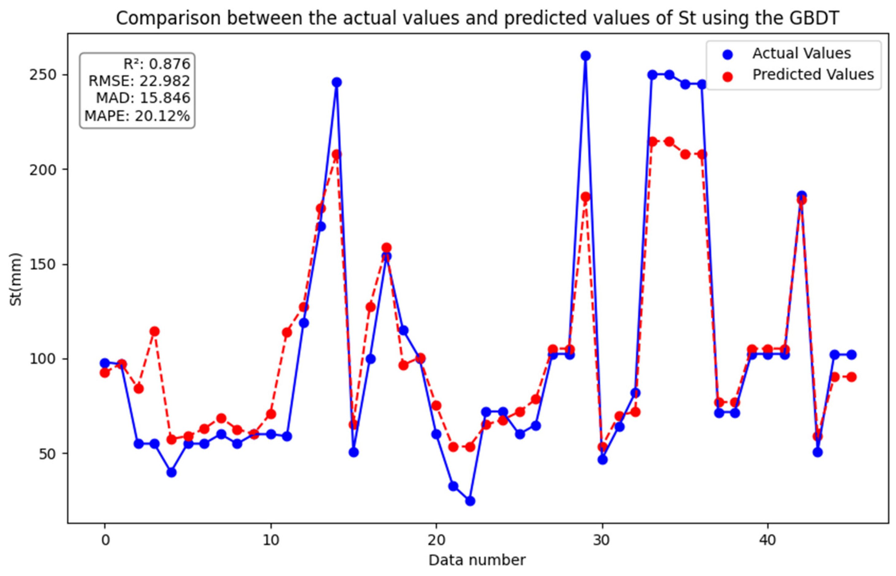
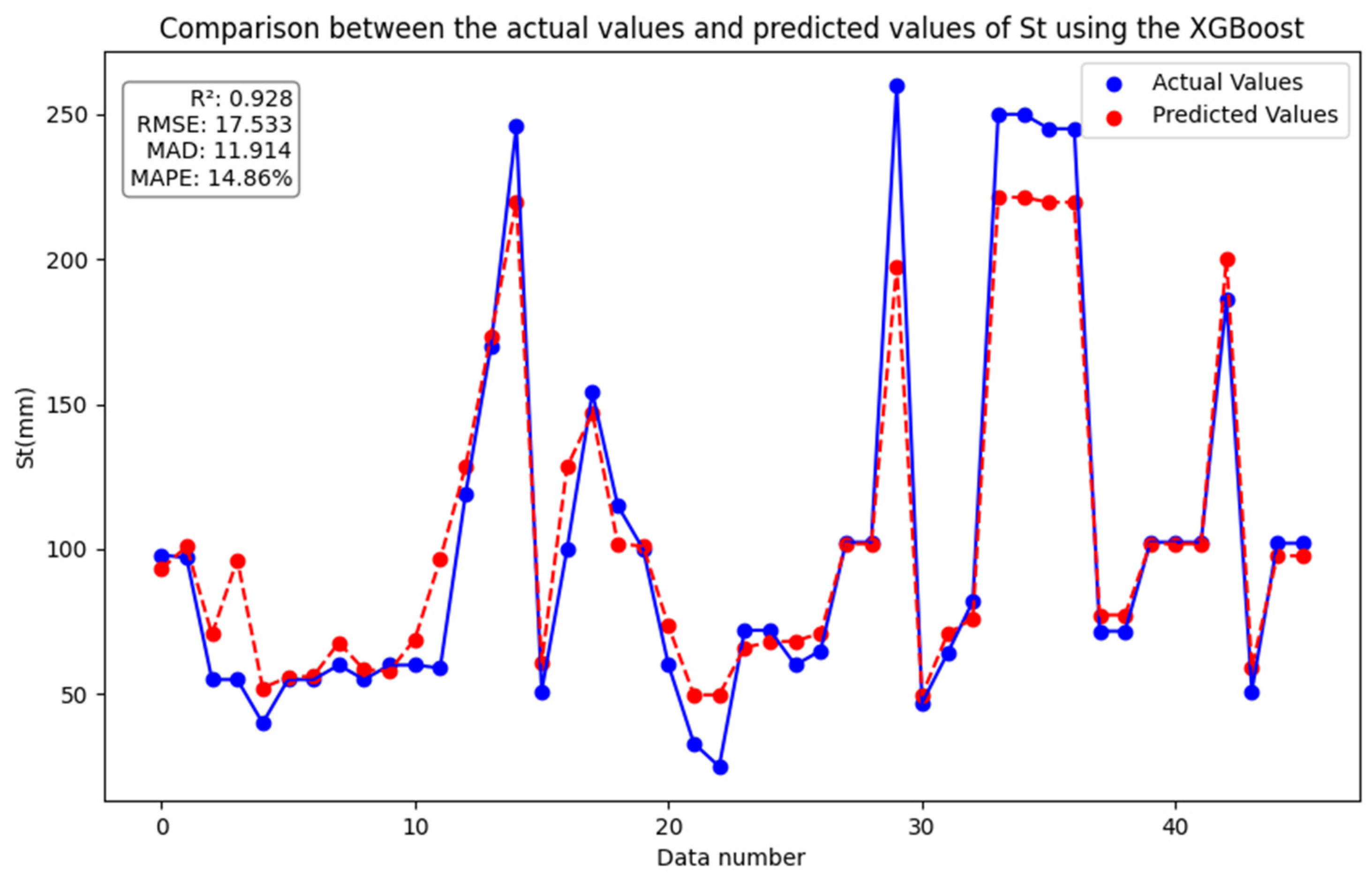
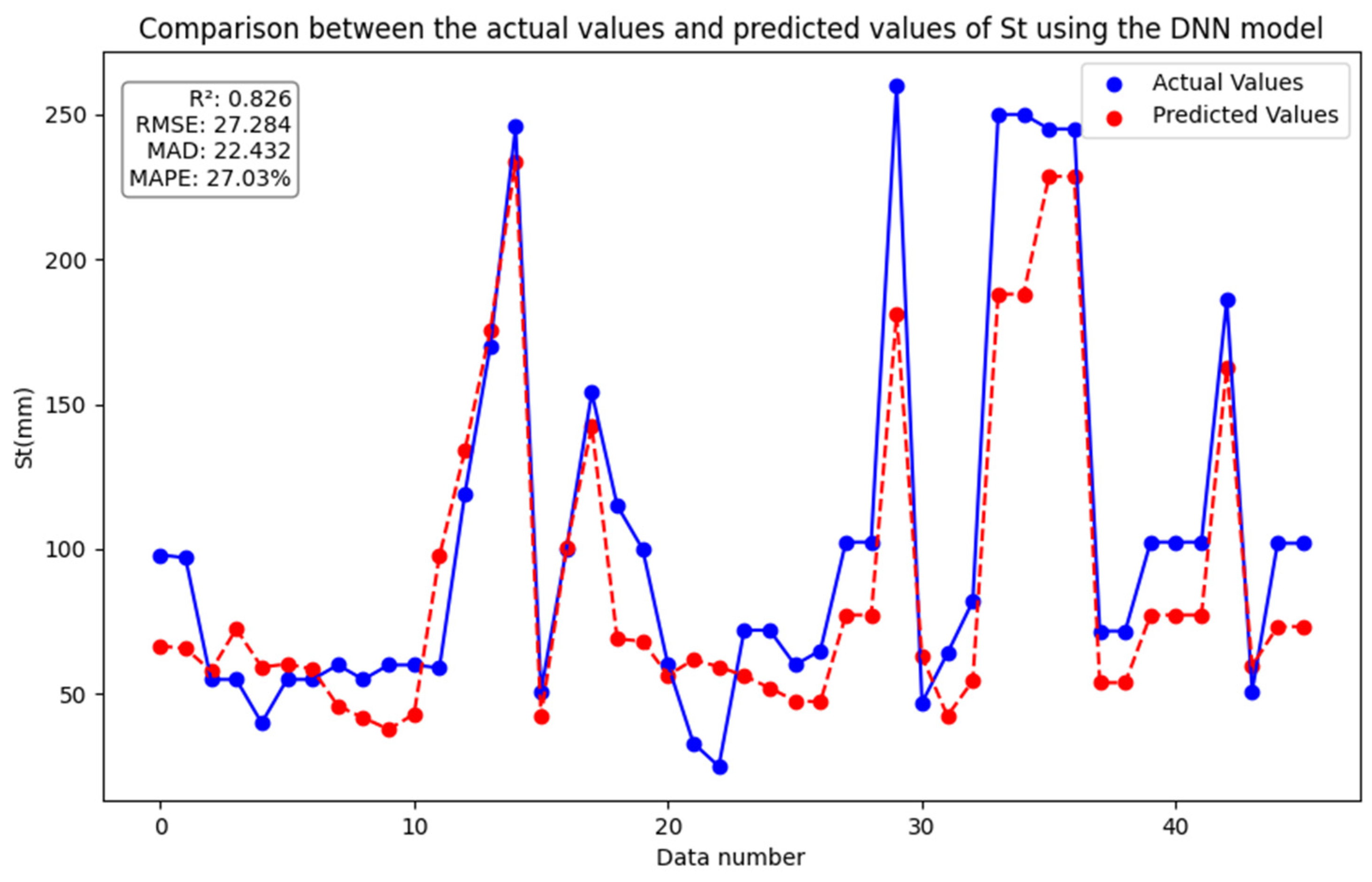
Figure 4, Figure 5 and Figure 6 show the results of predicting settlement St using the GBDT, XGBoost, and DNN models, respectively. In the figures, the blue curve represents the actual measured values, while the red curve represents the model predictions. In terms of performance metrics, the GBDT model achieved R 2 = 0.876, RMSE = 22.982, MAD = 15.846, and MAPE = 20.12%; the XGBoost model achieved R 2 = 0.928, RMSE = 17.533, MAD = 11.941, and MAPE = 14.86%; and the DNN model achieved R 2 = 0.826, RMSE = 27.284, MAD = 22.432, and MAPE = 27.03%. Across all evaluation metrics, the XGBoost model demonstrated superior performance. These metrics indicate that the XGBoost model can accurately predict settlement and possesses strong generalization ability. This may be because tree-based methods (GBDT and XGBoost) typically perform well when handling structured data and nonlinear relationships, whereas DNNs might be better suited for complex data such as images and text. Since predicting St in this task likely involves structured data, tree-based models have an advantage.

5.2.2. SVM Model and RF Model

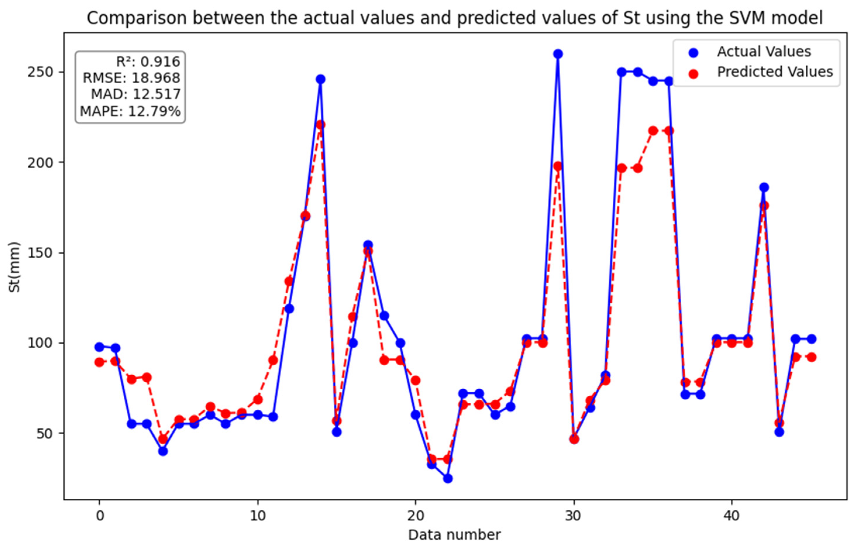
Figure 7 and Figure 8 show the results of predicting settlement St using the SVM model and the RF model, respectively. In terms of performance metrics, the SVM model’s prediction results are better, with R 2 = 0.916, RMSE = 18.968, MAD = 12.517, and MAPE = 12.79%. In comparison, the RF model’s prediction results are slightly inferior, with R 2 = 0.901, RMSE = 20.570, MAD = 13.458, and MAPE = 15.87%. SVM often performs well on small to medium-sized, low-dimensional datasets, especially when there is a clear boundary or a complex nonlinear relationship between features and the target variable (captured through kernel functions). The current results align with these characteristics.

5.2.3. Integrated Model

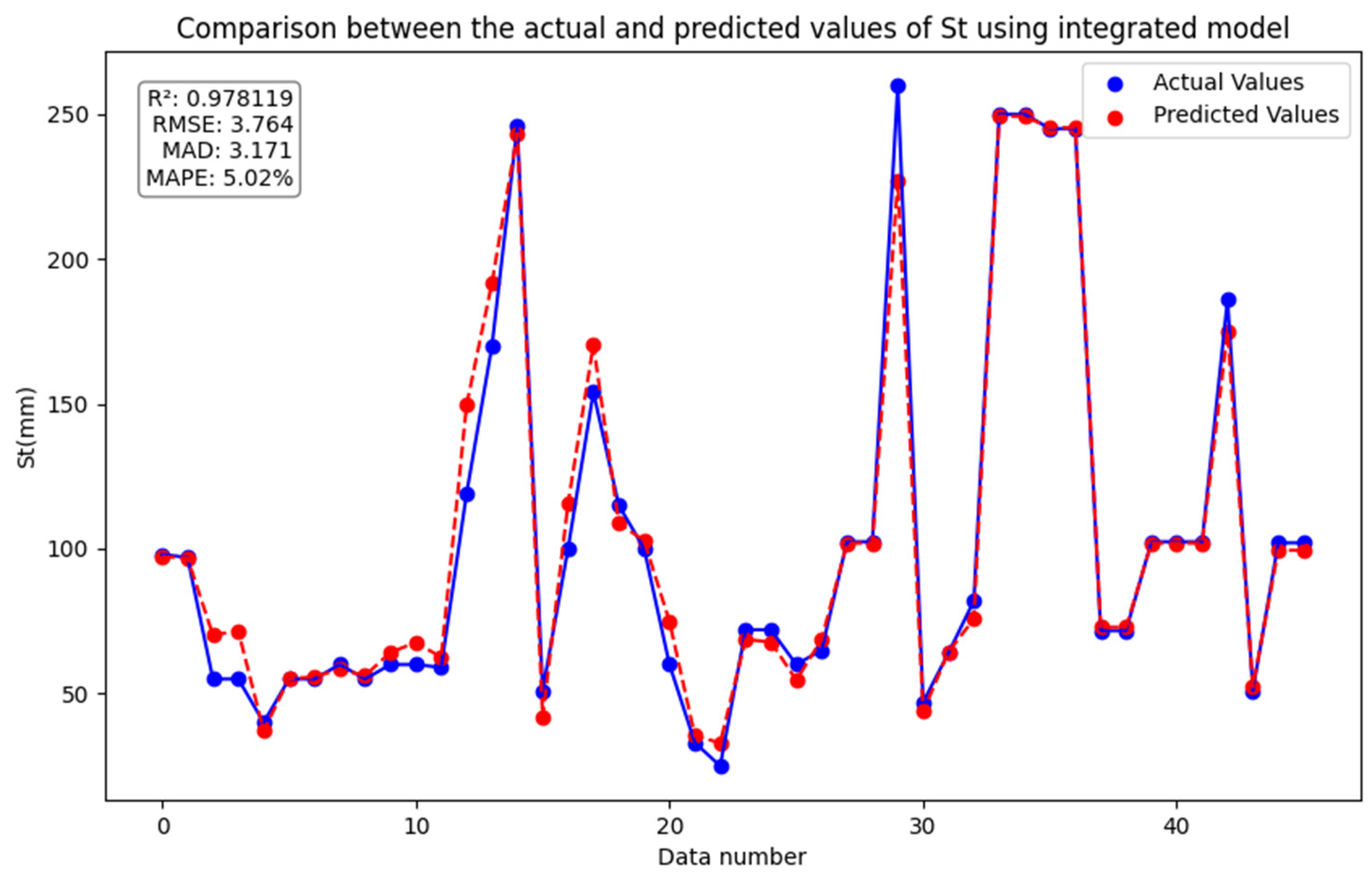
The prediction results of the SVM-integrated RF model are shown in Figure 9. The actual and predicted values almost coincide, indicating that the model’s predicted values are very close to the actual values, demonstrating a high degree of fit and prediction accuracy. Statistical indicators further confirm this, with R 2 = 0.978, RMSE = 3.764, MAD = 3.171, and MAPE = 5.02%, and performance based on the mean ± standard deviation of the outer folds of nested cross-validation: R 2 = 0.978 ± 0.05, RMSE = 3.764 ± 0.45, MAD = 3.171 ± 0.38, MAPE = 5.02% ± 0.32%. These results indicate that the multi-models established by the SVM-ensemble RF approach proposed in this study achieve very high data fit, perform well in handling complex ground settlement problems, effectively capture nonlinear relationships in the data, and provide high-precision predictions.
To provide a comprehensive model comparison, the nested cross-validation statistical results of this study are shown in the table below (all results are reported as mean ± standard deviation), as presented in Table 3. Specifically, the SVM-ensemble RF model’s metrics are significantly superior to those of the other five models, demonstrating very strong generalization ability and accuracy. The models ranked after the SVM-ensemble RF in terms of performance are XGBoost, SVM, RF, GBDT, and DNN, respectively. By combining the strengths of SVM and RF, the ensemble model can more effectively capture nonlinear relationships in the data and substantially reduce prediction error. The SVM performs excellently on high-dimensional data and complex nonlinear problems, while the RF has advantages in feature selection and resistance to overfitting. Integrating the two further improves the model’s predictive accuracy and stability.

5.3. Comparison Between the Integrated Model and the Existing Equations

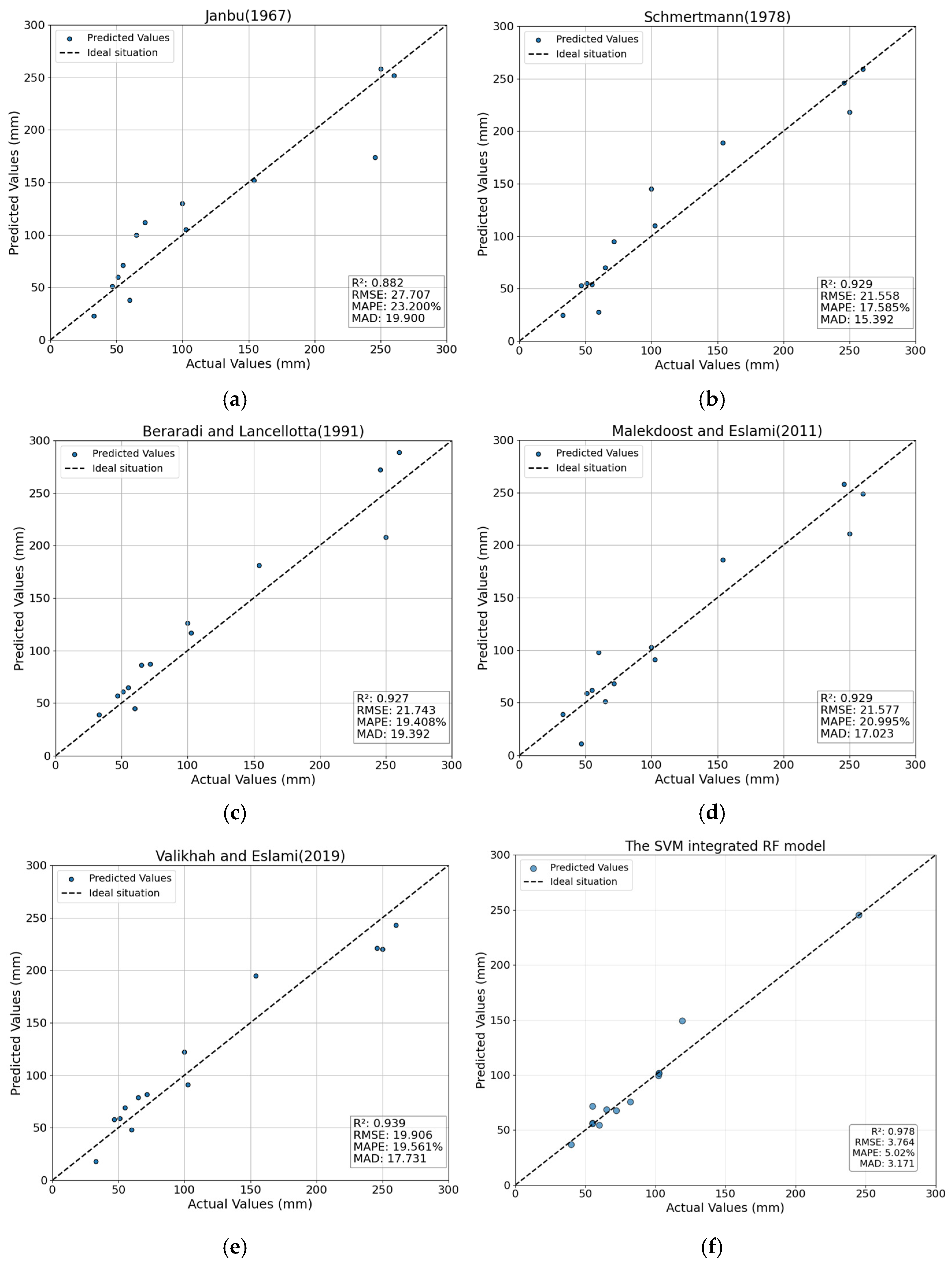
In this section, the SVM-ensemble RF model with the best predictive performance is selected and compared with traditional empirical formula prediction methods. Table 1 summarizes the comparison of traditional methods relying on empirical formulas, including the research results of Janbu (1967) [31], Schmertmann (1978) [32], Berardi and Lancelotta (1991) [33], Malekdoost and Eslami (2011) [34], and Valikhah and Eslami (2019) [3]. Thirteen out of the 46 datasets used in this study were randomly selected for validation. Figure 10 compares the prediction results of the previous method and SVM-integrated RF model, and provides R 2 , RMSE, MAD, and MAPE values for each method for quantitative comparison between the previous method and the current model.
As shown by the results in Figure 10, the SVM-integrated RF model significantly outperforms previous methods in prediction accuracy. For example, the integrated model proposed in this study has a mean absolute deviation (MAD) value of 3.171, which is much lower than the MAD values of earlier methods, indicating a clear advantage in prediction error. Additionally, the RMSE and MAPE values of the SVM-integrated RF model are also significantly lower than those of other methods, further confirming its high accuracy in settlement prediction. In contrast, traditional methods, which rely on empirical formulas or linear assumptions, struggle to fully capture complex nonlinear relationships, resulting in certain limitations in prediction performance. Notably, compared to previous approaches, the SVM-integrated RF model proposed in this study not only demonstrates superior prediction accuracy but also offers greater versatility and practicality. Traditional methods often entail complex calculations or depend on specific soil conditions, whereas the integrated model developed here leverages machine learning techniques to more efficiently handle multidimensional input parameters, simplifying the computation process. Furthermore, the SVM-integrated RF model is more flexible in its input parameter requirements, making it suitable for a wider range of geological conditions and engineering scenarios.

5.4. Uncertainty Analysis of Integrated Models

Since an SVM-integrated RF model introduces a human kernel function and the impact of the integrated model architecture on the prediction boundary remains unclear, along with the randomness in training and testing splits affecting the model’s stability, quantifying the uncertainty of the prediction model is crucial for improving the model’s credibility. This paper employs Monte Carlo Simulation (MCS) to quantify the uncertainty in the predictions of the proposed integrated model. Monte Carlo Simulation is a numerical method based on random sampling that generates predictive distributions by sampling the uncertainties in model parameters and structure, and further calculates the predictive mean, standard deviation, and confidence intervals, thereby providing a more comprehensive reference for model predictions.
Assuming the number of samples in the test set is N and the number of simulations is S, the dimension of the prediction matrix Y is N × S. The formulas for calculating the prediction mean, standard deviation, and confidence interval are given by Equations (18)–(20).
y ^ i = 1 S j = 1 S y i j , i = 1,2 , , N
σ i = 1 S 1 S y i j y ^ i 2 , i = 1,2 , , N
C I 95 % = y ^ i 1.96 · σ i , y ^ i + 1.96 · σ i
In this context, y ^ i represents the predicted mean, and y i j is the predicted value of the i-th sample in the j-th simulation. σ i is the standard deviation of the predictions, and C I 95 % refers to the 95% confidence interval, which represents the upper and lower bounds of the predicted value at a 95% confidence level. It provides a range of credibility for the predicted values.
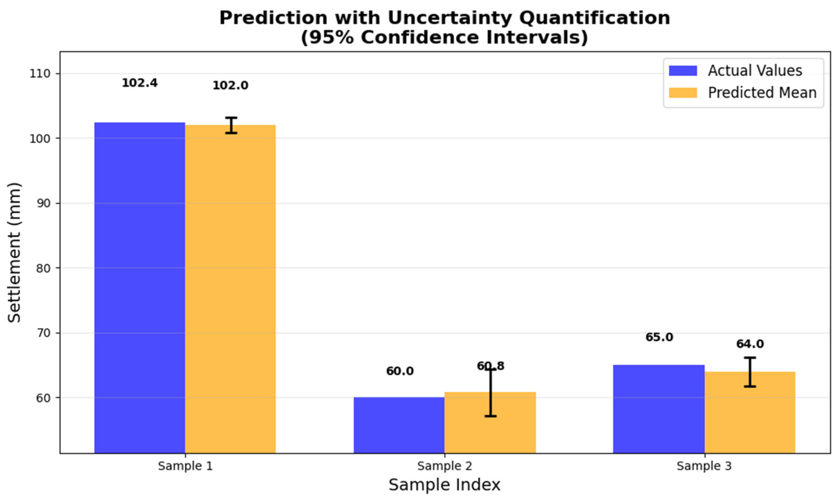
Through Monte Carlo simulation, this article quantified the uncertainty of the predicted results of the test set samples. Figure 11 shows the actual values, predicted mean, and 95% confidence interval of the test set samples. It can be seen from the figure that the predicted values of each sample are represented by a vertical interval, with the upper and lower bounds corresponding to the upper and lower limits of the confidence interval, respectively. The prediction intervals for sample 1 are [102.0, 102.4], sample 2 is [60.0, 60.8], and sample 3 is [64.0, 65.0]. The narrow confidence interval range of all samples indicates that the model has a high degree of certainty in predicting these samples. Further validated the accuracy of the integrated machine learning prediction model proposed in this study.

5.5. Sensitivity Analysis of Integrated Models

In order to comprehensively evaluate the impact of input variables on the prediction results of SVM-integrated RF model, this paper adopts two methods for sensitivity analysis of SVM-integrated RF model, namely feature importance analysis and SHAP (Shapley Additive exPlans) value. For feature importance analysis, we used model-based feature importance (through a random forest model) and custom perturbation analysis methods. For SHAP analysis, we used the SHAP library. Figure 12 presents the feature importance values of three input parameters in the model (foundation width B, foundation load q, and corrected cone tip resistance q t ). The results indicate that the feature importance value of B is 14.036, making it the variable with the greatest influence on the prediction results; followed by q, with a feature importance value of 5.0694; and q t , which has a feature importance value of 4.5948, indicating a relatively smaller impact. This suggests that foundation width B is the most critical input parameter in the model, contributing significantly more to the settlement prediction results than the other variables. In contrast, although q and q t also have some influence on the prediction results, their importance is significantly lower than that of B. This finding aligns with the physical mechanisms of foundation settlement, as foundation width directly affects the stress distribution and settlement of the foundation soil.
The second sensitivity analysis method used in this study is SHAP (Shapley Additive exPlans) value. Figure 13 shows the impact of quantifying three input parameters B, q, and q t using the SHAP method on the model results. From Figure 13, it can be seen that a higher B value has a positive impact on the model output, with a positive SHAP value, indicating that an increase in B will lead to an increase in the predicted value; A lower B value has a negative impact on the model output, and a negative SHAP value indicates that a decrease in B will lead to a decrease in the predicted value. This distribution characteristic is consistent with the physical mechanism of foundation settlement, as the width of the foundation directly affects the stress distribution and settlement of the foundation. A larger foundation width usually leads to greater settlement. In contrast, the SHAP values of ultimate loads q and q t have a narrower distribution, concentrated around 0, indicating that q and qt have a smaller impact on the model output. Although the variation in q has a certain impact on the prediction results, its influence range is limited, and its positive or negative contributions to the model output are relatively balanced. This is consistent with the previous analysis of feature importance, further verifying the secondary role of q and q t in the model.
To gain a deeper understanding of the nonlinear feature effects predicted by the model, we conducted partial dependence (PDP) and individual conditional expectation (ICE) analyses. Figure 14 shows the nonlinear influence mode of foundation width B and load q on settlement prediction. The PDP curve shows that the foundation width B exhibits a significant nonlinear effect on settlement prediction within the range of 0.5–2.0 m. When B increases from 0.5 m to about 1.2 m, the predicted settlement shows a rapid downward trend, with an average decrease of about 40%. After B > 1.2 m, the settlement prediction tends to stabilize, indicating a significant threshold effect of the foundation width effect. The ICE curve distribution shows significant heterogeneity in the response of different samples to changes in baseline width, with some samples exhibiting stronger width sensitivity. The influence of load q on settlement prediction exhibits stronger nonlinear characteristics. In the low load range (200–600 kPa), settlement growth is relatively gentle. After the load exceeds 600 kPa, settlement prediction shows an accelerated growth trend, reflecting typical nonlinear soil response. The dispersion degree of ICE curve in the load dimension is relatively small, indicating a high consistency of load effects among different samples. These findings provide important theoretical basis for optimizing basic dimensions and load control in engineering practice, demonstrating the superior performance of ensemble learning models in capturing nonlinear characteristics of complex geotechnical problems.

6. Model Validation

In order to verify the generalization capability of the integrated model proposed in this study, this section employs a Generative Adversarial Network (GAN) to generate 50 new datasets based on 46 groups of data collected from the literature. This study used the open-source library CTGAN (version 0.8.0) to generate synthetic data. The model training is set to 2000 cycles, with a batch size of 100, and automatically identifies discrete variables in the dataset to ensure that the generated table data conforms to the original data structure. The GAN comprises two main components: a generator and a discriminator. The generator (G) is responsible for generating “fake” data in an attempt to make it indistinguishable from real data, while the discriminator (D) is tasked with determining whether the input data is real (from the actual dataset) or generated by the generator (fake). The objective of the GAN is to minimize the loss of the generator while maximizing the loss of the discriminator, which can be formalized as follows:
m i n G m a x D V D , G = E ~ P d a t a x log D x + E ~ z ~ P z z log 1 D G z
where x represents real data and z represents random noise.
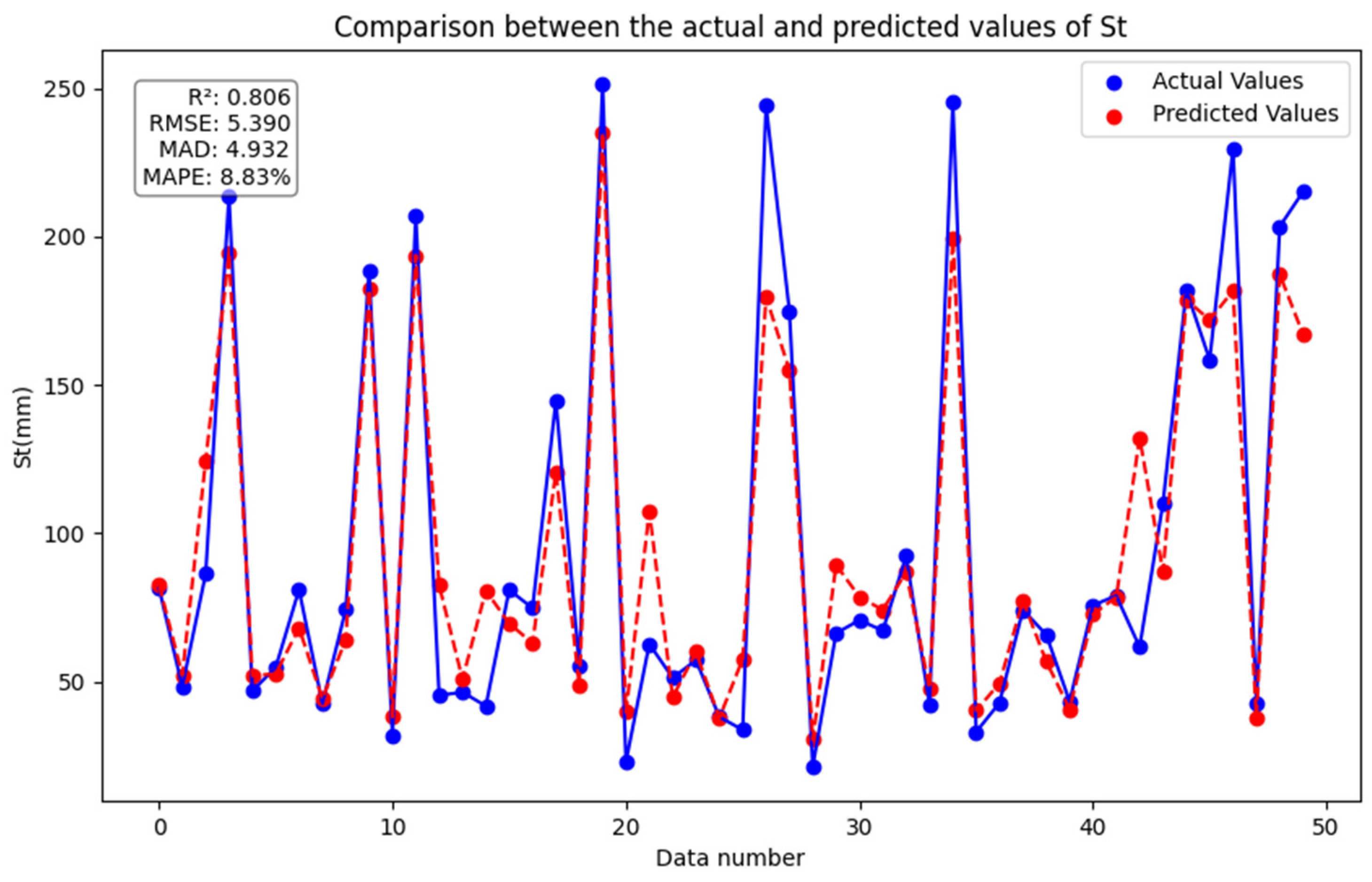
Figure 15 shows the prediction results of the integrated model on 50 newly generated datasets by GAN, with R 2 = 0.806, RMSE = 5.390, MAD = 4.932, and MAPE = 8.83%. The errors are relatively small and the prediction results are satisfactory, indicating that the integrated model proposed in this study has good generalization ability.
To improve the authenticity of the generated data, we have taken the following steps: (1) In GAN training, we used adversarial loss functions and regularization techniques to encourage alignment between the generated data and the real data distribution; (2) Compare the distribution similarity between generated data and real data through statistical tests (such as K-S test); (3) Based on domain knowledge, visual inspection and validation of key parameter ranges were conducted on the generated data to ensure that it conforms to physical meaning. We emphasize that GAN generated data is only used for auxiliary validation and does not replace real data testing. In future work, we will expand the real dataset to improve model reliability.

7. Conclusions

This study utilized 46 sets of data collected from the literature to establish DNN, SVM, and RF models and an ensemble model for predicting shallow foundation settlement, and compared the predictive performance of each model. The following are the main conclusions and discussions of this study:
(1)
The SVM-ensemble RF model proposed in this study predicts values that closely match the actual values and outperforms the other models, followed by XGBoost, SVM, RF, GBDT, and DNN. Therefore, the proposed ensemble model has very high predictive capability and can effectively capture the complex nonlinear relationships between soil layer characteristics and settlement.
(2)
This study compared the SVM-ensemble RF model with traditional methods and single machine learning models. The results showed that the SVM-ensemble RF model performed best across all evaluation metrics. This further validates that the integrated model proposed in this study can achieve more realistic and accurate settlement predictions, providing a reference for geotechnical engineering practice.
(3)
This study employs Monte Carlo simulation to quantify the uncertainty of the ensemble model’s prediction results and conducts a sensitivity analysis. The results of uncertainty quantification all fall within the 95% confidence interval. The sensitivity analysis shows that, when using an SVM-integrated RF model to predict settlement values (St), the foundation width (B) has the greatest influence, followed by foundation load (q), and finally corrected cone tip resistance ( q t ).
(4)
Finally, based on the 46 sets of data collected from the literature, 50 new datasets were generated using a Generative Adversarial Network (GAN) and applied to the ensemble model proposed in this study. The results indicate that the ensemble model demonstrates good generalization ability.
Based on the aforementioned research content, future studies could explore how to integrate more types of data (such as remote sensing data and seismic data) with existing models. Through data fusion, a more comprehensive description of the characteristics of the foundation soil layers can be achieved, thereby improving the accuracy and applicability of predictions. Additionally, by utilizing big data technologies and cloud computing platforms, large-scale datasets can be processed and analyzed more effectively, enhancing the model’s generalization capability. Furthermore, while ensuring prediction accuracy, research should focus on simplifying the model structure to improve its computational efficiency and interpretability. Uncertainty analysis and prior assessments can also be incorporated into the model to enhance the reliability and practicality of the prediction results.

Author Contributions

Conceptualization, R.Z. and W.Z.; Methodology, R.Z. and W.Z.; Software, R.Z. and W.Z.; Validation, R.Z. and W.Z.; Formal analysis, R.Z. and W.Z.; Investigation, R.Z. and W.Z.; Resources, W.Z.; Data curation, R.Z. and W.Z.; Writing—original draft, R.Z. and W.Z.; Writing—review & editing, R.Z. and W.Z.; Visualization, R.Z. and W.Z.; Supervision, W.Z.; Project administration, W.Z.; Funding acquisition, W.Z. All authors have read and agreed to the published version of the manuscript.

Funding

This work was supported by the National Natural Science Foundation of China (No. 52468054), the Qinghai Provincial Science and Technology Cooperation Project (No. 2023-HZ-806) and the Fund of China Scholarship Council (No. 202308630007).

Institutional Review Board Statement

Not applicable.

Informed Consent Statement

Not applicable.

Data Availability Statement

The data presented in this study are available on request from the corresponding author.

Conflicts of Interest

The authors declare that they have no known competing financial interests or personal relationships that could have appeared to influence the work reported in this paper.

References

  1. Holtz, R.D.; Kovacs, W.D.; Sheahan, T.C. An Introduction to Geotechnical Engineering; Prentice-hall: Englewood Cliffs, NJ, USA, 1981. [Google Scholar]
  2. Paikowsky, S.G.; Fu, Y.; Amatya, S.; Canniff, M.C. Uncertainty in shallow foundations settlement analysis and its utilization in SLS design specifications. In Proceedings of the 17th International Conference on Soil Mechanics and Geotechnical Engineering (Volumes 1, 2, 3 and 4), Alexandria, Egypt, 5–9 October 2009; pp. 1317–1320. [Google Scholar]
  3. Valikhah, F.; Eslami, A. CPT-Based Nonlinear Stress–Strain Approach for Evaluating Foundation Settlement: Analytical and Numerical Analysis. Arab. J. Sci. Eng. 2019, 44, 8819–8834. [Google Scholar] [CrossRef]
  4. Omer, J.R.; Delpak, R.; Robinson, R.B. A new computer program for pile capacity prediction using CPT data. Geotech. Geol. Eng. 2006, 24, 399–426. [Google Scholar] [CrossRef]
  5. Moshfeghi, S.; Eslami, A. Reliability-based assessment of drilled displacement piles bearing capacity using CPT records. Mar. Georesources Geotechnol. 2019, 37, 67–80. [Google Scholar] [CrossRef]
  6. Robertson, P.K. Soil behaviour type from the CPT: An update. In Proceedings of the 2nd International Symposium on Cone Penetration Testing, Huntington Beach, CA, USA, 9–11 May 2010; Volume 2, pp. 575–583. [Google Scholar]
  7. Mayne, P.W. Cone Penetration Testing; Transportation Research Board: Washington, DC, USA, 2007. [Google Scholar]
  8. Lunne, T.; Powell, J.J.M.; Robertson, P.K. Cone Penetration Testing in Geotechnical Practice; CRC Press: Boca Raton, FL, USA, 2002. [Google Scholar]
  9. Jefferies, M.G.; Davies, M.P. Use of CPTU to estimate equivalent SPT N 60. Geotech. Test. J. 1993, 16, 458–468. [Google Scholar] [CrossRef]
  10. Samui, P. Support vector machine applied to settlement of shallow foundations on cohesionless soils. Comput. Geotech. 2008, 35, 419–427. [Google Scholar] [CrossRef]
  11. Kaveh, A. Applications of Artificial Neural Networks and Machine Learning in Civil Engineering; Studies in Computational Intelligence; Springer: Cham, Switzerland, 2024; Volume 1168. [Google Scholar]
  12. Kourehpaz, P.; Molina Hutt, C. Machine learning for enhanced regional seismic risk assessments. J. Struct. Eng. 2022, 148, 04022126. [Google Scholar] [CrossRef]
  13. Ahmed, M.O.; Khalef, R.; Ali, G.G.; El-Adaway, I.H. Evaluating deterioration of tunnels using computational machine learning algorithms. J. Constr. Eng. Manag. 2021, 147, 04021125. [Google Scholar] [CrossRef]
  14. Faraz Athar, M.; Khoshnevisan, S.; Sadik, L. CPT-Based Soil Classification through Machine Learning Techniques. In Proceedings of the Geo-Congress 2023, Los Angeles, CA, USA, 26–29 March 2023; pp. 277–292. [Google Scholar]
  15. Bentéjac, C.; Csörgő, A.; Martínez-Muñoz, G. A comparative analysis of gradient boosting algorithms. Artif. Intell. Rev. 2021, 54, 1937–1967. [Google Scholar] [CrossRef]
  16. Ester, M.; Kriegel, H.P.; Xu, X. XGBoost: A scalable tree boosting system. In Proceedings of the 22nd ACM SIGKDD International Conference on Knowledge Discovery and Data Mining, San Francisco, CA, USA, 13–17 August 2016; pp. 785–794. [Google Scholar]
  17. Schmidhuber, J. Deep learning in neural networks: An overview. Neural Netw. 2015, 61, 85–117. [Google Scholar] [CrossRef]
  18. Hastie, T.; Tibshirani, R.; Friedman, J. The Elements of Statistical Learning: Data Mining, Inference, and Prediction; Springer: New York, NY, USA, 2009. [Google Scholar]
  19. Breiman, L. Random forests. Mach. Learn. 2001, 45, 5–32. [Google Scholar] [CrossRef]
  20. Ho, T.K. Random decision forests. In Proceedings of the 3rd International Conference on Document Analysis and Recognition, Montreal, QC, Canada, 14–16 August 1995; Volume 1, pp. 278–282. [Google Scholar]
  21. Cervantes, J.; Garcia-Lamont, F.; Rodríguez-Mazahua, L.; Lopez, A. A comprehensive survey on support vector machine classification: Applications, challenges and trends. Neurocomputing 2020, 408, 189–215. [Google Scholar] [CrossRef]
  22. Friedman, J.H. Greedy function approximation: A gradient boosting machine. Ann. Stat. 2001, 29, 1189–1232. [Google Scholar] [CrossRef]
  23. Asgarkhani, N.; Kazemi, F.; Jankowski, R.; Formisano, A. Dynamic ensemble-learning model for seismic risk assessment of masonry infilled steel structures incorporating soil-foundation-structure interaction. Reliab. Eng. Syst. Saf. 2025, 267, 111839. [Google Scholar] [CrossRef]
  24. Benker, M.; Furtner, L.; Semm, T.; Zaeh, M.F. Utilizing uncertainty information in remaining useful life estimation via Bayesian neural networks and Hamiltonian Monte Carlo. J. Manuf. Syst. 2021, 61, 799–807. [Google Scholar] [CrossRef]
  25. Padarian, J.; Minasny, B.; McBratney, A.B. Assessing the uncertainty of deep learning soil spectral models using Monte Carlo dropout. Geoderma 2022, 425, 116063. [Google Scholar] [CrossRef]
  26. Nguyen, H.T.T.; Cao, H.Q.; Nguyen, K.V.T.; Pham, N.D.K. Evaluation of explainable artificial intelligence: Shap, lime, and cam. In Proceedings of the FPT AI Conference, Ha Noi, Vietnam, 6–7 May 2021; pp. 1–6. [Google Scholar]
  27. Lundberg, S.M.; Erion, G.G.; Lee, S.I. Consistent individualized feature attribution for tree ensembles. arXiv 2018, arXiv:1802.03888. [Google Scholar]
  28. Cracknell, M.J.; Reading, A.M. Geological mapping using remote sensing data: A comparison of five machine learning algorithms, their response to variations in the spatial distribution of training data and the use of explicit spatial information. Comput. Geosci. 2014, 63, 22–33. [Google Scholar] [CrossRef]
  29. Wang, W.; Xue, C.; Zhao, J.; Yuan, C.; Tang, J. Machine learning-based field geological mapping: A new exploration of geological survey data acquisition strategy. Ore Geol. Rev. 2024, 166, 105959. [Google Scholar] [CrossRef]
  30. Ishihara, K.; Yoshimine, M. Evaluation of settlements in sand deposits following liquefaction during earthquakes. Soils Found. 1992, 32, 173–188. [Google Scholar] [CrossRef]
  31. Janbu, N. Settlement Calculations Based on the Tangent Modulus Concept; Technical University of Norway: Trondheim, Norway, 1967. [Google Scholar]
  32. Schmertmann, J.H. Guidelines for Cone Test, Performance, and Design; Report FHWA-TS-78209; Federal Highway Administration: Washington, DC, USA, 1978; p. 145. [Google Scholar]
  33. Berardi, R.; Lancellotta, R. Stiffness of granular soils from field performance. Geotechnique 1991, 41, 149–157. [Google Scholar] [CrossRef]
  34. Malekdoost, M.; Eslami, A. Application of CPT data for estimating foundations settlement-case histories. Sharif J. Civ. Eng. 2011, 1, 75–85. [Google Scholar]
  35. MolaAbasi, H.; Saberian, M.; Khajeh, A.; Li, J.; Chenari, R.J. Settlement predictions of shallow foundations for non-cohesive soils based on CPT records-polynomial model. Comput. Geotech. 2020, 128, 103811. [Google Scholar] [CrossRef]
  36. Eslami, A.; Gholami, M. Bearing capacity analysis of shallow foundations from CPT data. In Proceedings of the 16th International Conference on Soil Mechanics and Geotechnical Engineering, Osaka, Japan, 12–16 September 2005; pp. 1463–1466. [Google Scholar]
  37. Mayne, P.W.; Illingworth, F. Direct CPT method for footing response in sands using a database approach. In Proceedings of the 2nd International Symposium on Cone Penetration Testing, Huntington Beach, CA, USA, 9–11 May 2010. [Google Scholar]
  38. Briaud, J.L.; Gibbens, R. Behavior of five large spread footings in sand. J. Geotech. Geoenviron. Eng. 1999, 125, 787–796. [Google Scholar] [CrossRef]
  39. Eslami, A.A.; Gholami, A.M. Analytical model for the ultimate bearing capacity of foundations from cone resistance. Sci. Iran. 2006, 13, 223–233. [Google Scholar]
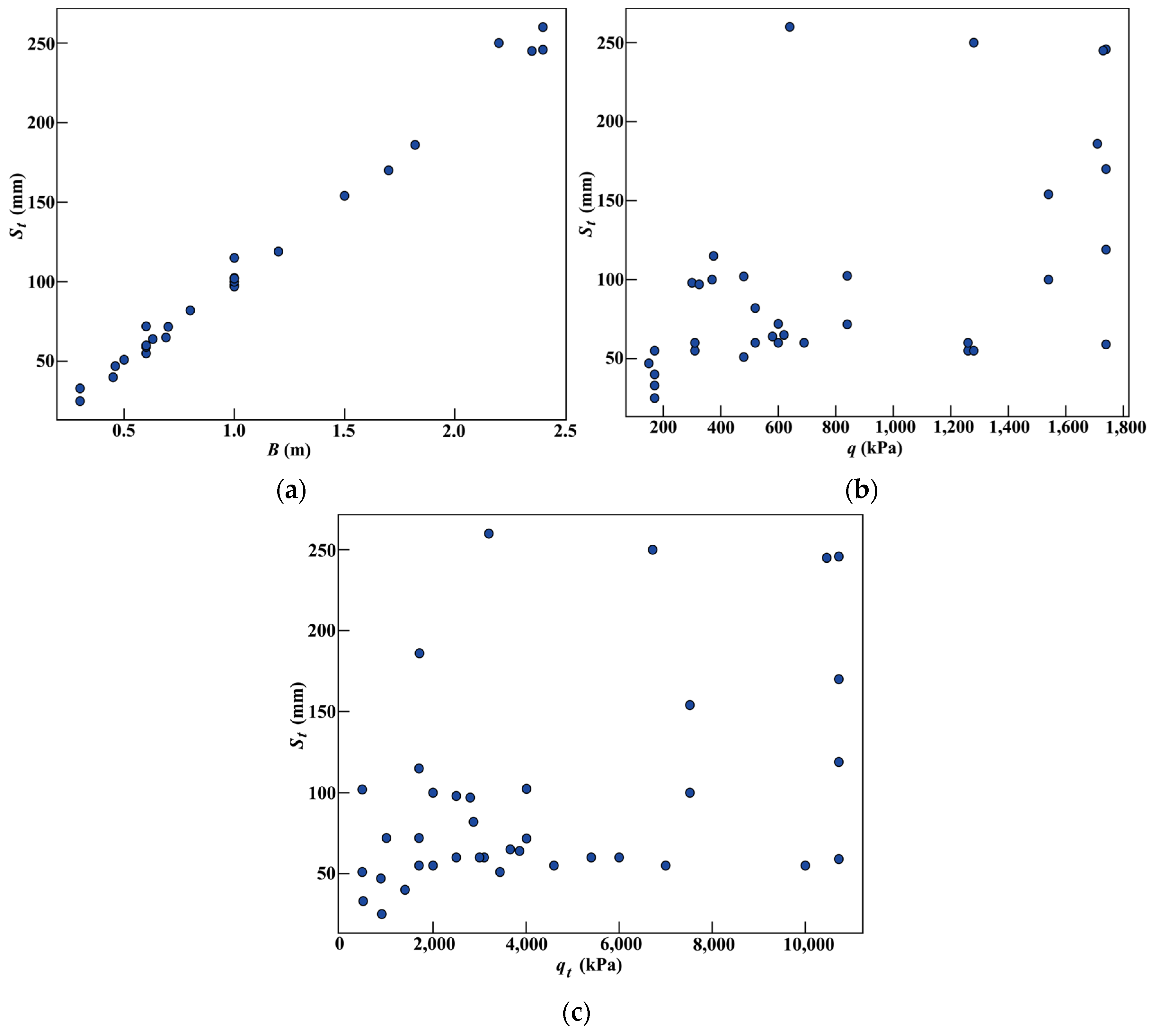
Figure 1. The relationship between input and output parameters. (a) B- S t ; (b) q- S t ; (c) q t - S t .
Applsci 15 12174 g001
Figure 2. Structure of the DNN Model.
Applsci 15 12174 g002
Figure 3. Algorithm of SVM-integrated RF model to estimate the settlement of the foundation.
Applsci 15 12174 g003
Figure 4. Comparison between the actual values and predicted values of St using the GBDT.
Applsci 15 12174 g004
Figure 5. Comparison between the actual values and predicted values of St using the XGBoost.
Applsci 15 12174 g005
Figure 6. Comparison between the actual values and predicted values of St using the DNN Model.
Applsci 15 12174 g006
Figure 7. Comparison between the actual values and predicted values of St using the SVM model.
Applsci 15 12174 g007
Figure 8. Comparison between the actual values and predicted values of St using the RF model.
Applsci 15 12174 g008
Figure 9. Comparison between the actual values and predicted values of St using the SVM-integrated RF method.
Applsci 15 12174 g009
Figure 10. Comparison between the actual and predicted St by previous methods and the current model. (a) Janbu (1967) [31]; (b) Schmertmann (1978) [32]; (c) Berardi and Lancellotta (1991) [33]; (d) Malekdoost and Eslami (2011) [34]; (e) Valikhah and Eslami (2019) [3]; (f) The SVM-integrated RF model.
Applsci 15 12174 g010
Figure 11. Quantifying uncertainty in prediction results of the test set using Monte Carlo methods.
Applsci 15 12174 g011
Figure 12. Visualization of feature importance for the three input parameters B, q and q t .
Applsci 15 12174 g012
Figure 13. Quantify the impact of three input parameters on the model results using SHAP method.
Applsci 15 12174 g013
Figure 14. The Mechanism of Influence of Foundation Width and Load on Settlement Prediction Based on PDP and ICE.
Applsci 15 12174 g014
Figure 15. Comparison between the actual values and predicted values of St for GAN-generated data using the SVM-integrated RF method.
Applsci 15 12174 g015
Table 1. The calculation method for foundation settlement proposed by predecessors.
NoMethodsEquationRemarks
1Janbu (1967) [31] S t = 1 m j σ 0 + σ σ r j σ 0 σ r j × H S t : foundation settlement,
ε : strain induced by effective stress increase,
σ 0 : initial effective stress,
σ : increase in effective stress under applied stress,
m: modulus number,
H: the thickness of the target layer,
j: stress exponent = 0.5,
σ r : constant stress equal to 100 kPa
2Schmertmann (1978) [32] S t = C 1 C 2 q 0 2 B I z E H C 1 : a correction factor for the depth of foundation embedment = 1 0.5 σ 0 q ,
C 2 : a correction factor to account for creep in soil (t is time in year) = 1 0.2 log t 0.1 ,
I z : strain influence factor, E = 2 q c
3Berardi and Lancellotta (1991) [33] S t = q B E I s E = K E σ r σ 0 + σ 2 σ r 0.5 , K E : modulus number,
I s = 0.63, 0.69, and 0.88 for circle, square, and rectangular foundations, respectively
4Malekdoost and Eslami (2011) [34] S t = 1 m j σ 0 + σ σ r j σ 0 σ r j × H m = 2 q c ,
j = q c 1 + 0.05 log q c × R f 2 5 log q c 11 R f + R f 2 ,
q c : cone tip resistance,
R f : friction ratio = f s q c
5Valikhah and Eslami (2019) [3] S t = 1 m j σ 0 + σ σ r j σ 0 σ r j × H m = 0.25 b × 2 B + 1 3 B 3 × q c ,
B: foundation width,
b: penetration cone diameter,
j = q c x + y q c , x = 0.02 R f + 0.5 , y = 7.53 σ 0 0.25
Table 2. A summary of the data employed in this research.
Soil TypeCase No.Footing Shape q t
(kPa)
R f D f (m)B
(m)
q
(kPa)
S t (mm)Reference
Silt1Square25000.50130098Eslami and Gholami (2005) [36]
2 28000.50132597
Silt Sand3Square70000.500.6126055
4 10,0000.500.6128055
Silt Clay5Circular14000.600.4517040
6 17000.600.617055
7 20000.600.617055
Silt Clay8Circular31000.61.50.652060
9 46000.61.50.631055
10 54000.61.50.631060
11 60000.61.50.669060
Glaciofluvial Sand12Rectangular10,7200.510.40.6174059Mayne and Illingworth (2010) [37]
13 10,7200.510.61.21740119
14 10,7200.510.81.71740170
15 10,7200.511.12.41740245.8
Siliceous Sand16Square34400.440.50.548051
Sand, Silty Sand17Square75200.650.7611540100Briaud and Gibbens (1999) [38]
18 75200.650.761.51540154
Silt19Square17000.501375115Eslami and Gholami (2006) [39]
20 20000.501370100
Silt Sand21Square30000.500.6126060
Silt Clay22Circular5000.600.317033
23 9000.600.317025
Silt Clay24Circular10000.61.50.660072
25 17000.61.50.660072
26 25000.61.50.660060
White Fine Sand27Square36600.5400.6962065Mayne and Illingworth (2010) [37]
Glaciofluvial Sand28Rectangular40100.6301840102.4
29 40100.6301840102.4
30 32000.631.12.4640260
Compacted Fill31Square8800.5300.4615047
32 38600.4800.6358064
33 28700.5800.852082
Alluvial Sand34Circular67200.62.22.21280250
35 67200.62.22.21280250
36 10,4600.522.352.351730245
37 10,4600.522.352.351730245
Dune Sand38Square40100.6600.784071.7
39 40100.6600.784071.7
40 40100.6601840102.4
41 40100.6601840102.4
42 40100.6601840102.4
Silty Sand43Circular17100.550.61.821710186
Siliceous Dune Sand44Square4800.440.50.548051
45 4800.4411480102
46 4800.4411480102
Table 3. Comparison of nested cross validation performance of GBDT, XGBoost, DNN, SVM, RF, and SVM-integrated RF models (mean ± standard deviation).
Model R 2 RMSEMADMAPE
GBDT0.876 ± 0.00922.982 ± 0.4315.846 ± 0.4320.12% ± 0.40%
XGBoost0.926 ± 0.00717.533 ± 0.4811.914 ± 0.3914.86% ± 0.35%
DNN0.826 ± 0.01527.284 ± 0.6822.432 ± 0.5227.03% ± 0.48%
SVM0.916 ± 0.00818.968 ± 0.5212.517 ± 0.4112.79% ± 0.38%
RF0.901 ± 0.01220.570 ± 0.6113.458 ± 0.4915.87% ± 0.45%
SVM-integrated RF0.978 ± 0.0053.764 ± 0.453.171 ± 0.385.02% ± 0.32%
Disclaimer/Publisher’s Note: The statements, opinions and data contained in all publications are solely those of the individual author(s) and contributor(s) and not of MDPI and/or the editor(s). MDPI and/or the editor(s) disclaim responsibility for any injury to people or property resulting from any ideas, methods, instructions or products referred to in the content.