Article

Landslide Susceptibility Mapping Optimization for Improved Risk Assessment Using Multicollinearity Analysis and Machine Learning Technique

by
Buddhi Raj Joshi
1,2,
Netra Prakash Bhandary
2,*,
Indra Prasad Acharya
3,
Niraj KC
4 and
Chakra Bhandari
5
1
School of Engineering, Faculty of Science and Technology, Pokhara University, Kaski 33700, Nepal
2
Faculty of Collaborative Regional Innovation, Ehime University, Matsuyama City 790-8577, Japan
3
Department of Civil Engineering, Pulchowk Campus, Institute of Engineering, Tribhuvan University, Lalitpur 44700, Nepal
4
Department of Geomatics Engineering, Pashchimanchal Campus, Institute of Engineering, Tribhuvan University, Kaski 33700, Nepal
5
Madan Bhandari College of Engineering, Madan Bhandari Memorial Academy Nepal, Urlabari 56604, Nepal
*
Author to whom correspondence should be addressed.
Appl. Sci. 2025, 15(22), 12152; https://doi.org/10.3390/app152212152
Submission received: 26 September 2025 / Revised: 9 November 2025 / Accepted: 13 November 2025 / Published: 16 November 2025

Abstract

This study integrates geospatial modeling with multi-criteria decision analysis for an improved approach to landslide susceptibility mapping (LSM). This approach addresses key challenges in LSM through sophisticated multicollinearity analysis and machine learning strategies. We compared three machine learning models for weighting, and of them the Permutation-Weighted model yielded the best prediction results, with an Area Under Curve (AUC) of 95%, an accuracy of 69%, and a recall of 66%. To resolve perfect multicollinearity (r = 1) between land use land cover (LULC) and geological factors, we implemented Principal Component Analysis (PCA). The selected factors demonstrated strong predictive power, with the PCA-derived features exhibiting the best performance, having a Variation Inflation Factor (VIF) of 1.004. Slope appeared as the most influential factor (51.7% contribution), while the Topographic Wetness Index (TWI) was less dominant with only 6.6%. Multiple landslide susceptibility mapping methods yielded consistent results, with 29.8–30.1% of the study area showing moderate susceptibility and 35.2–36.9% in the high to very high susceptibility class. The model also incorporated vulnerability parameters weighted by the United Nations Office for Disaster Risk Reduction (UNDRR) indicators, including farmland, buildings, bare land, water bodies, roads, and amenities to generate hazard, vulnerability, and risk maps. The results were verified through visual comparison with high-resolution Google Earth imagery. The Permutation-Weighted model performed better than others, categorizing 12.4% at high-risk, while Random Forest (RF) categorized 7.2% at high risk. This study makes three key contributions: (1) It establishes the effectiveness of PCA/VIF for variable selection, (2) it provides a comparison of machine learning weighting techniques, and (3) it validates a workflow applicable to data-scarce regions.

1. Introduction

Landslides represent one of the most devastating natural hazards globally, causing significant human casualties, economic losses, and environmental degradation each year [1,2]. In mountainous regions such as the Himalayas, the convergence of active tectonics, steep topography, intense monsoon rainfall, and expanding human settlement creates a perfect storm for landslide disasters [3,4]. The frequency and magnitude of these events are being further amplified by climate change, which causes more extreme precipitation patterns, as well as by ongoing anthropogenic pressures such as road construction and deforestation on unstable slopes [5,6].
The Doti District in Nepal’s Far-Western region epitomizes these challenges. This region has experienced recurrent and catastrophic landslide events, resulting in severe consequences. For instance, heavy monsoon rains in August 2015 triggered landslides in Toleni and Daud, resulting in six fatalities, displacing over 250 families, and causing extensive damage to crop and vital infrastructure [7]. Subsequent incidents highlight systemic vulnerabilities; in April 2018, government-built rehabilitation houses in geologically unstable areas were rendered uninhabitable by landslides, underscoring critical failures in land-use planning [8]. More recently, landslides in July 2020 in Sayal Rural Municipality displaced multiple families, and a June 2021 event in Jorayal blocked the crucial Bhimdutta Highway, severing supply lines to seven districts [9,10]. These recurring disasters demonstrate an urgent need for scientifically robust landslide risk assessment and management strategies tailored to this specific region.
In response to such risks, Landslide Susceptibility Mapping (LSM) has emerged as a fundamental tool for identifying areas prone to slope failure. A wide range of methodologies has been applied in the Himalayan context, ranging from qualitative heuristic approaches [11] to quantitative statistical models such as Logistic Regression and Weights of Evidence [12,13], and more recently, advanced Machine Learning (ML) techniques like Random Forest (RF) and Support Vector Machines [14,15]. These ML models are particularly valued for their ability to handle complex, non-linear relationships between landslide causative factors. Studies in similar Himalayan terrains, such as in Sindhupalchok and Darjeeling, have demonstrated the superior predictive power of RF models [16,17]. However, despite these technological advances, the reliable application of LSM for risk assessment in data-scarce regions like Doti faces several persistent challenges.
First, severe multicollinearity among geomorphological predictors (e.g., between slope, elevation, and Topographic Wetness Index) can destabilize ML models and lead to unreliable feature importance rankings, thereby misrepresenting the true causative mechanisms [18,19]. Second, conventional weighting approaches within LSM, especially for categorical variables like geology and land use, often rely on expert opinion, introducing subjectivity and limiting the model’s reproducibility and transferability across different regions [20,21]. Third, a significant gap exists in effectively integrating geophysical hazard data with socioeconomic vulnerability parameters to produce a comprehensive risk assessment. Many existing models remain purely physio-centric, lacking the robust integration of field-validated vulnerability data necessary for practical disaster risk reduction planning [22,23]. These challenges are particularly acute in developing countries like Nepal, where detailed landslide inventories and high-resolution geospatial data are often unavailable or incomplete [24,25].
This study aims to overcome these limitations by proposing a novel, integrated machine learning framework for LSM and risk assessment in the Doti District. The specific objectives are (1) to systematically address predictor multicollinearity using Principal Component Analysis (PCA) and Variation Inflation Factor (VIF) analysis; (2) to compare and optimize factor weighting through objective ML techniques, namely Random Forest (version 1.4.0) Gini Importance and Permutation Importance (both implemented using Scikit-learn, an open-source library), thereby eliminating subjective bias; and (3) to generate a holistic landslide risk map by integrating the optimized susceptibility model with vulnerability parameters based on United Nations Office for Disaster Risk Reduction (UNDRR) indicators.
The theoretical significance of this research lies in its methodological contribution to optimizing LSM through rigorous statistical treatment of data and comparative ML weighting strategies [26,27]. From an application perspective, this study provides the first detailed, quantitatively robust landslide susceptibility and risk assessment for the Doti District. The proposed framework is designed to be replicable in other data-scarce Himalayan regions, offering a scientifically rigorous yet practical decision-support tool [28,29]. It is expected to assist local authorities in immediate disaster prevention, long-term land-use planning, and sustainable development, ultimately contributing to enhanced resilience in this highly vulnerable community [30,31]. Recent advances in ensemble sample selection [32] and transfer learning [33] offer promising solutions for data-scarce regions, while the specific influence of factors like NDVI requires careful consideration in model design [34].

2. Materials and Methods

2.1. Study Area

The study area lies in the Doti District of Nepal’s Far-Western region (Figure 1a) and has been subject to recurrent severe landslide events (Figure 1b I–IV). In August 2015, intense rainfall triggered landslides in Toleni and Daud, resulting in six deaths, displacement of over 250 families, and major loss of farmland and infrastructure (Section C-I) [7]. Similar issues have continued over the years. In April 2018, newly constructed government resettlement housing became uninhabitable due to unstable terrain (Section C-II) [8]. In July 2020, landslides in Sayal Rural Municipality displaced several households and placed many more at high risk (Section C-III) [9]. In June 2021, another landslide in Jorayal blocked the Bhimdutta Highway, disrupting essential supply routes to multiple districts (Section C-IV) [10]. These recurring events highlight persistent gaps in land-use planning and disaster risk governance, disproportionately affecting vulnerable communities such as the Haliyas. Therefore, a coordinated strategy that combines immediate response with long-term risk reduction is urgently needed in landslide-prone areas of Doti.
Geological and topographic conditions create high landslide susceptibility in the study area [35]. The region lies in a tectonically active zone between the Khaptad Gneiss Klippe to the north and the Dandeldhura Crystallines to the south, with intervening Doti Schist formations [36]. Major tectonic faults (MCT, MBT, and MFT), resulting from the ongoing India-Eurasia collision, transect the area [37]. The November 2022 Doti earthquake (Mw 5.6) provided recent evidence of this activity, triggering slope failures through ground shaking [37].
Topographically, Doti District shows ideal conditions for mass wasting due to various reasons. Elevations range from 289 to 3281 m (Figure 1b) across the Mid-Hill range, with over 80% of slopes exceeding 15 degrees. Climatic conditions further increase landslide risk. Seasonal monsoon rainfall averages 670.7 mm from July to November, interacting with elevation-dependent zones ranging from tropical (<1000 m) to subalpine (>3000 m) [38]. Major north–south flowing rivers, the Seti and Budhi Ganga, dissect the terrain. This landscape limits arable land to only 19.55%, yet 90% of the farming population remains highly vulnerable to landslides [39]. Therefore, systematic landslide risk assessment is essential for this Himalayan region, given the combined threats of steep slopes, seismic activity, and human-induced stressors.

2.2. Computational Framework and Implementation

The entire analytical workflow for this study was implemented using a combination of specialized software and programming libraries. All statistical computations, multicollinearity assessments, including Principal Component Analysis (PCA) and Variation Inflation Factor (VIF) calculation, and Machine Learning Modeling (MLM) were conducted using Python programming environment (version 3.9). The analysis leveraged key scientific computing libraries, including Scikit-learn (v 1.0) for machine learning algorithms, with the Random Forest model specifically configured with 100 decision trees (n_estimators = 100), Gini impurity criterion, and otherwise default parameters to ensure reproducibility. SciPy (v 1.7) was employed for statistical testing and correlation analysis, while Pandas (v 1.3) with NumPy (v 1.20) handled comprehensive data manipulation and numerical computations. For geospatial data processing, cartography, and map generation, the study utilized ArcGIS 10.8 alongside QGIS 3.22, ensuring robust spatial analysis and high-quality visualization outputs throughout the study.

2.3. Landslide Inventory: Compilation and Validation

The landslide inventory was compiled as a point dataset in ESRI shapefile format, containing 1112 landslide locations with each point representing the centroid of an identified landslide scar (Figure 2).
Comprehensive field verification was not feasible due to the remote and inaccessible terrain. All landslide locations were rigorously validated through visual interpretation of high-resolution Google Earth imagery at a 1:50 scale. Landslide identification was based on clear geomorphological indicators, including main scraps, exposed soil/bedrock, and characteristic hummocky deposition zones. For comparison, an equal number of non-landslide points (1112) were systematically selected from areas showing no visual evidence of slope instability, with consistent vegetation cover and stable terrain characteristics observed over multiple years. This well-established and reliable methodology is suitable for landslide inventory development in data-scarce regions. This ensures a reliable comparison between unstable and stable terrain. Finally, division was made on both landslide and non-landslide points into 80% for training and 20% for testing using a simple random sampling technique. This standard procedure prevents bias in model evaluation.
The selection of these twelve causative factors was based on their established importance in landslide literature and data availability at a regional scale. While other potential variables like detailed lithological units, daily rainfall intensity, Normalized Difference Moisture Index (NDMI), and proximity to geological faults are acknowledged contributors to slope stability, they were excluded from this analysis. This decision was primarily due to the lack of consistently available, high-resolution spatial data for these parameters across the entire study area. This study intended to develop a model reliant on commonly available and standardized datasets to ensure the framework’s practicality and transferability to other data-scarce Himalayan regions.

2.4. Landslide Causative Factors: Standardization and Normalization

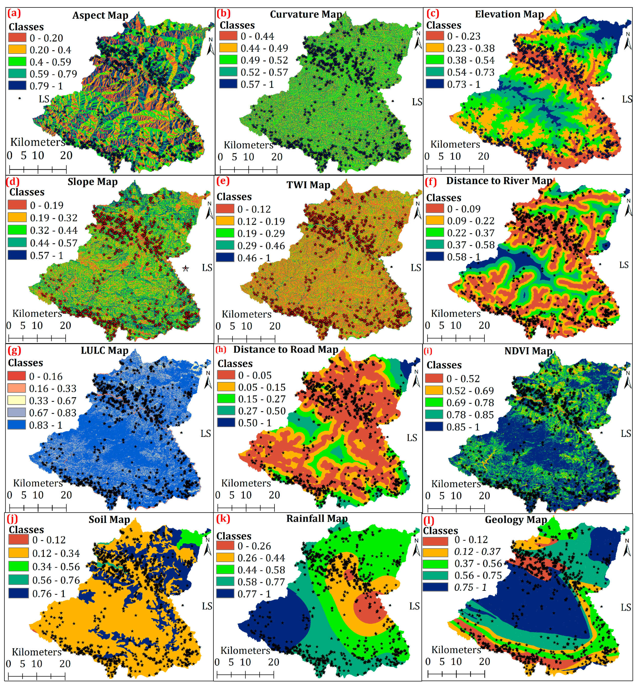
The precise identification and analysis of landslide causative factors is a basic requirement for reliable landslide susceptibility mapping. For this study, we selected twelve critical landslide causative factors, all of which were validated through earlier research [40,41,42]. ASTER Global DEM data generated five topographic factors: aspect, curvature, elevation, slope, and TWI (Figure 3a–e). The river/stream data from the Department of Survey Nepal has been derived in vector format at a scale of 1:50,000 for buffer zone generation (Figure 3f). Furthermore, this study used 30 m resolution land use/land cover (LULC) classification data from ICIMOD (2019) (Figure 3g). The necessary road network data was obtained from OpenStreetMap (OSM) at a mapping scale of 1:25,000 to ensure proper spatial positioning (Figure 3h). Additionally, NDVI maps were derived from 30 m resolution Landsat 8 satellite imagery (Figure 3i). At a scale of 1:250,000, the SOTER Nepal database provides vector-based delineated soil types that represent the best nationwide detail available for analyzing soil classifications within the study area. To systematically analyze slope stability conditions, the proximity study for roads and rivers relied on 100 m intervals through their buffer zones (Figure 3j). The Department of Hydrology and Meteorology (DHM) provided the study area with 20-year rainfall distribution data having a spatial resolution of 5 km, which stands for long-term precipitation patterns (Figure 3k). The Department of Mines and Geology provided geological data with a scale ratio of 1:1,000,000 (Figure 3l).
The study used WGS 1984 UTM Zone 44N as the common coordinate system to ensure uniformity across all validated causative factors during processing (Figure 3a–l). Furthermore, Proper analysis and integration required the spatial data standardization process at a 30-m resolution for all causative factors (Figure 3a–l). The conversion of categorical variables into numeric values used Weight of Evidence (WoE)-based label encoding to identify weighted ranking scales that reflect their landslide impacts (see Table A1). All continuous variables were normalized using min-max scaling to ensure equal weighting in the landslide susceptibility analysis while eliminating unit differences. The standard formula used to execute the normalization procedure is as in Equation (1) [43].
N o r m a l i z e d   V a l u e = X X m i n X m a x X m i n
where X represents the original value, and Xmin and Xmax are the minimum and maximum values in the dataset, respectively. The precise preprocessing method of landslide causative factors creates standardized conditions that enhance the reliability of landslide susceptibility mapping.

2.5. Multicollinearity Assessment

This study employed three analytical methods to verify that the selected landslide causative factors function independently, as confirmed throughout a comprehensive multicollinearity assessment.

2.5.1. Correlation Analysis

The evaluation of potential multicollinearity between continuous landslide causative factors required a Pearson correlation analysis for measuring linear relationships between variable pairs. The Pearson correlation coefficient (r) measures the linear relationships between factors X and Y and is calculated using Equation (2) [44].
r X Y = i = 1 n   X i X Y i Y i = 1 n     X i X 2 i = 1 n   Y i Y 2
The formula calculates correlation using n observations, which include Xi individual values and Yi individual values, as well as mean variables X and Y . The linear dependence between two variables ranges from −1 to +1, representing perfect negative to perfect positive correlation, respectively. A conservative |r| < 0.7 threshold was applied to identify meaningful inter-factor correlations because statistical value ranges above 0.7 signify that more than 49% (r2 > 0.49) of one variable derives from another variable based on established geospatial modeling standards. The analysis was using the Python SciPy library, generating a correlation heatmap to visualize relationships among the twelve conditioning factors. The approach was adopted to solve landslide susceptibility mapping issues by removing multicollinearity yet keeping the principal factors that enhance the quality of susceptibility assessment.
In this study, a conservative Pearson correlation coefficient threshold of |r| < 0.7 was employed to identify significant multicollinearity, as values exceeding this threshold indicate that over 49% of variance (r2 > 0.49) in one variable is explained by another, which could destabilize model coefficients [45]. This primary screening was complemented by Variation Inflation Factor (VIF) analysis, where variables with VIF > 5 were iteratively removed, retaining only factors with VIF < 3 in the final model to ensure predictor independence.

2.5.2. Principal Component Analysis (PCA)

Following correlation analysis that identified highly correlated variables ∣ r i j ∣ ≥ 0. Principal Component Analysis (PCA) was applied to the reduced dataset Xreduced to transform the correlated variables into decorrelated principal components. The transformation was performed using Equation (3) [46]:
Z = X r e d u c e d × W  
where W comprises the eigenvectors of the covariance matrix Cov (Xreduced). The eigenvalues (λ_i) were derived by solving the characteristic equation det (Σ−λI) = 0, where Σ represents the covariance matrix of standardized predictors. The proportion of variance explained by each principal component was then calculated as V a r i a n c e i = λ _ i λ _ k × 100 % . This approach successfully generated principal components with a diagonal covariance matrix, confirming complete decorrelation and elimination of multicollinearity, while preserving essential information through components capturing significant variance proportions.

2.5.3. Variation Inflation Factor (VIF) Analysis

In this study, the evaluation of multicollinearity for landslide causative factors continued through the calculation of VIF for all causative factors. VIF estimation for causative factors involved the use of Equation (4) [33].
V I F i = 1 1 R i 2
The statistical analysis method relies upon R i 2 to figure out the value of the coefficient of determination that results from regressing a single variable against a set of other causative factors. The first phase of iterative analysis of selected variables exceeded a VIF value of 5 because their variance reached 80% due to co-occurring predictive variables. The study employed iterative variable elimination to remove multicollinear predictors, retaining only variables with VIF values < 3. Through this analytical process, the landslide susceptibility model achieved minimal multicollinearity. Python statistical packages executed this operation to sustain causative factors with meaningful physical aspects and reduce duplicate relationships in the dataset. The final predictor set consisted of statistically independent variables owning geologically relevant characteristics for developing reliable landslide susceptibility models.

2.6. Feature Importance Analysis

The assessment of different causative factors that affect landslide susceptibility used the Random Forest (RF) and Permutation Importance as an effective method. This section presents the mathematical expression together with the system execution procedures.

2.6.1. Random Forest Feature Importance (Gini Importance)

Random Forest figures out feature importance through Gini Importance calculations, also known as Mean Decrease in Impurity. The importance of feature ‘f’ within a forest with trees ‘T’ is decided as per Equation (5) [47].
R F   Importance   f = 1 T t = 1 T   n N t   Δ G i n i n , f
where
N_t = Set of all nodes in tree t
Gini(n) = Gini impurity at node n
ΔGini(n,f) = Reduction in Gini impurity at node n when split on feature f
T = Total number of trees in the random forest
f = Feature being evaluated
The calculation of Gini Importance used a Random Forest classifier with 100 trees to analyze the feature matrix (X) and target variable (y). The Random Forest Importance (f) score obtained for feature (f) showed an average of its Gini impurity reduction (ΔGini (n, f)) measured across all nodes and trees through rf_ model feature importance. Scoring features higher by this approach shows their better ability to form splits and decrease impurity, but such a method tends to prioritize features with large cardinality values. This method delivers a dependable first assessment of predictor importance to guide landslide susceptibility mapping, although it may show potential bias.

2.6.2. Permutation Importance

The addition of Permutation Importance to RF importance provides a method to assess landslide model accuracy changes through random value shuffling of features. Permutation importance calculation of the feature ‘f’ was calculated with R repetitions according to Equation (6) [48].
P e r m I m p o r t a n c e f = 1 R r 1 R   S c o r e original   S c o r e permuted   f , r
The Permutation Importance algorithm performed random value shuffles of features ten times, with unaffected other variable values to calculate average performance reduction versus baseline scores. The Scikit-learn Python library used for calculating permutation importance (f) provides an implementation to measure feature influence through mean performance decrease and feature reliability through the standard deviation decrease, while low deviation shows stable predictive importance. This method improves upon Gini Importance by avoiding high-cardinality feature bias through direct accuracy measurement of individual predictors. Additionally, the standard deviation was calculated across repetitions to decide Permutation Importance stability using Equation (7) [49].
σ f = 1 R r 1 R       Score   original   S c o r e permuted   f , r P e r m I m p o r t a n c e f 2
A high Permutation Importance score (Perm Importance(f)) shows the feature’s strong influence on model performance. The accompanying standard deviation (σf) measures consistency: low σf values denote stable, reliable importance across shuffles, while high σf suggests variable impact, potentially due to feature interactions, noise, or randomness. This dual metric (importance score ± variability) helps distinguish robust predictors from those requiring further investigation.

2.6.3. Combined Average Importance

The average feature importance, derived from uniting RF and Permutation Importance calculations for more trustworthy ranking capabilities, can be calculated using Equation (8) [50].
Average   Importance   f = R F   Importance   f + P e r m I m p o r t a n c e f 2
Random Forest (Gini) Importance and Permutation Importance, when used together, provide an effective combination for causative factor evaluation. The frequency of split identification from RF Importance comes with a trade-off because it gives undue weight to features with numerous categories. Permutation Importance calculates predictive impact directly, requires significant computational power because it lacks this bias. The average of these methods minimizes specific problem points of RF and stabilizes permutation importance calculations through a combined method. The combination leads to an improved and simpler feature ranking system for landslide susceptibility mapping.

2.7. Landslide Susceptibility Mapping

The integrated method was used for landslide susceptibility mapping, in which Random Forest with Permutation Importance metrics were combined to determine weights of the landslide causative factors and were used directly in the susceptibility mapping. The implementation details are described in the following subheadings.

2.7.1. Random Forest Weight Calculation

The application of class weights is a critical methodological step for mitigating the bias introduced by class imbalance, thereby enhancing model robustness by ensuring adequate consideration of minority classes during training. RF importance scores underwent conversion to percentage weights through mathematical transformation using Equation (9) [47].
W R F f = R F   Importance   f i 1 n     R F   Importance   f i × 100
where W R F ( f ) stands for the percentage contribution of the factor f among all features.

2.7.2. Permutation Importance Weight Calculation

Permutation importance evaluates a feature by observing what happens to the model when the feature’s information is corrupted. If the model becomes much worse, it is heavily relying on that feature. The Permutation importance values were normalized using Equation (10) [50].
W Perm   f =   Permutation   Importance   f i 1 n       Permutation   Importance   f i × 100
The converted data maintains original rankings, permitting direct method comparison.

2.7.3. Combined Weight Derivation

Combining Gini and Permutation importance is not standard practice because they operate on fundamentally different principles. Their separate assessment yields a richer, more nuanced feature analysis. Though a combined average weight was computed using Equation (11) [51].
W Combined   f = W R F f + W Perm   f 2
Random Forest Gini Importance scores were merged with Permutation Importance scores to create WCombined(f) for a weighted overlay model through equal weight application and normalization to 0–100 values. The combined approach compensates for each method’s limitations. The weighting accuracy of Permutation Importance eclipses Gini Importance because it directly assesses model performance, while the latter defaults to high-cardinality features. Measurement reliability can be assessed by calculating the standard deviation of permutation importance scores. The combination of two performance metrics delivers more unbiased feature ranking than traditional expert assessments and weights features based on their landslide impact level. The weighted factors achieve statistical validity combined with practical utility in landslide susceptibility mapping because they strike an equilibrium between operational efficiency and geomorphological significance.

2.8. Model Evaluation and Validation

The machine learning models were evaluated using various performance indicators on a test dataset of 200 samples. The model’s classification accuracy was calculated using standard statistical formulas (Equations (12)–(17)). Accuracy represents the proportion of correctly classified samples (both true positives and true negatives) out of the total samples (Equation (12)). Precision quantifies the proportion of true positives among all positive predictions (Equation (13)), while recall (sensitivity) measures the model’s ability to identify all actual positives (Equation (14)). The F1-score, calculated as the harmonic mean of precision and recall, provides a balanced measure of the model’s performance (Equation (15)). The true positive rate (TPR) and false positive rate (FPR) were computed, which are essential for generating the Receiver Operating Characteristic (ROC) curve, using Equations (16) and (17), respectively. Finally, ROC analysis was performed by comparing TPR and FPR across different classification thresholds to comprehensively assess model performance [52,53].
Accuracy = T P + T N T P + T N + F P + F N
Precision = T P T P + F P
Recall = T P T P + F N  
F 1 - score = 2 ×   Precision × Recall     Precision   +   Recall  
T P R = T P T P + F N
F P R = F P F P + T N
A true positive (TP) occurs when a model correctly identifies a positive instance. Conversely, a true negative (TN) occurs when the model correctly identifies a negative instance. A false positive (FP) is an error where the model incorrectly classifies a negative instance as positive. A false negative (FN) is the opposite error, where a positive instance is incorrectly classified as negative. The performance of the diagnostic models was evaluated using the Area Under the Receiver Operating Characteristic (AUC-ROC) curve. This curve plots the True Positive Rate (TPR) against the False Positive Rate (FPR) across different classification thresholds [33,52].

2.9. Landslide Risk Assessment

The multiplicative risk model for landslide assessments combines three vital elements, namely Hazard (H), Vulnerability (V), and Exposure (E), to figure out the final risk (R). Risk assessment at its final stage requires the multiplication operation between H, V, and E using Equation (18) [54].
R = H × V × E
This method ensures transparent, reproducible landslide risk assessments with physically interpretable results, while its adjustable component weights permit scenario-based analyses adaptable to diverse regional settings.
A landslide hazard indicates the intensity of the likelihood of the movement occurring in a specific geographical area based on the consequences of LSM results. The analysis begins with landslide susceptibility score clipping using the first percentile value (Q1) and the 99th percentile value (Q99) to prevent extreme values from controlling the analysis.

2.9.1. Clipping and Normalization

The LSM values undergo clipping along Q1 and Q99 percentiles to remove analysis errors that are caused by outliers. Equation (19) calculates the normalized hazard score (Hnorm) [55].
H n o r m = L S M clipped   Q 1 L S M Q 99 L S M Q 1 L S M
The hazard values are adjusted through this formula to span from 0 to 1, with minimal values at 0 and maximum values at 1.

2.9.2. Quantile Classification

The normalized hazard values are then classified into five hazard categories using quantile thresholds (Q20, Q40, Q60, Q80) as indicated in Equation (20) [56].
H class   = 1   Very   Low   0 H norm   < Q 20 2   Low   Q 20 H norm   < Q 40 3   Medium   Q 40 H norm   < Q 60 4   High   Q 60 H norm   < Q 80 5   Very   High   Q 80 H norm   1
Landslide hazards were classified into five categories (Very Low to Very High) by using a quantile distribution. The vulnerability assessment (V) evaluated areas’ exposure to landslide impacts by analyzing the presence of key elements. These elements included buildings, roads, amenities, farmland, vegetated areas, and bare land. Each element is represented as a binary raster, where a value of 1 indicates presence and 0 indicates absence.
Based on UNISDR (now UNDRR) criteria, importance weight was assigned to each element according to their relative potential for human and socioeconomic impact. The building sector received the highest weight (0.82) due to direct human occupancy and economic value, followed by roads (0.55) for connectivity and emergency access, schools and hospitals (0.45) as critical facilities, farmland (0.35) for livelihood security, vegetation (0.30) for environmental stability, and bare land (0.25) [57,58] representing lower direct vulnerability. This systematic weighting structure combines the physical exposure of elements with their associated social impacts to analyze overall vulnerability. The calculation of vulnerability follows the weighted addition of each vulnerability factor’s binary raster data as in Equation (21) [59].
V = i = 1 6   w i R i
where w i is the weight is, the factor, i as assigned above, R i is the binary raster standing for the presence (1) or absence (0) of the factor. This study evaluated risk zones by integrating vulnerability and exposure assessments for residential buildings, roads, amenities, farmland, and land cover. The vulnerability assessment followed UNISDR guidelines, assigning weights to elements based on their damage potential. Buildings received the highest weight (0.82) due to their human occupancy and economic value, followed by roads (0.55), amenities (0.45), and other components [57,58]. The exposure analysis identified buildings and critical infrastructure as top priorities (0.90) based on their location within hazard zones.
All elements were converted into a binary presence/absence raster, applied weighted summation, and normalized the results. The final risk map used quantile thresholds to classify areas into five risk categories, from Very Low to Very High. This standardized GIS-based methodology effectively combines geophysical hazard data with socioeconomic vulnerability analysis, providing a practical tool for decision-making in risk mitigation.
The risk values transition through five categories through the application of quantile thresholds (Q20, Q40, Q60, Q80). The final grouping of risks consists of the following categories as in Equation (22) [56].
R class   = 1   Very   Low   0 R norm   < Q 20 2   Low   Q 20 R norm   < Q 40 3   Medium   Q 40 R norm   < Q 60 4   High   Q 60 R norm   < Q 80 5   Very   High   Q 80 R norm   1
From the obtained final risk map, High-risk areas ( R class > 4) are recognized for further analysis and field verification efforts.

3. Results

3.1. Multicollinearity Analysis and Estimating Weightage

3.1.1. Multicollinearity Analysis

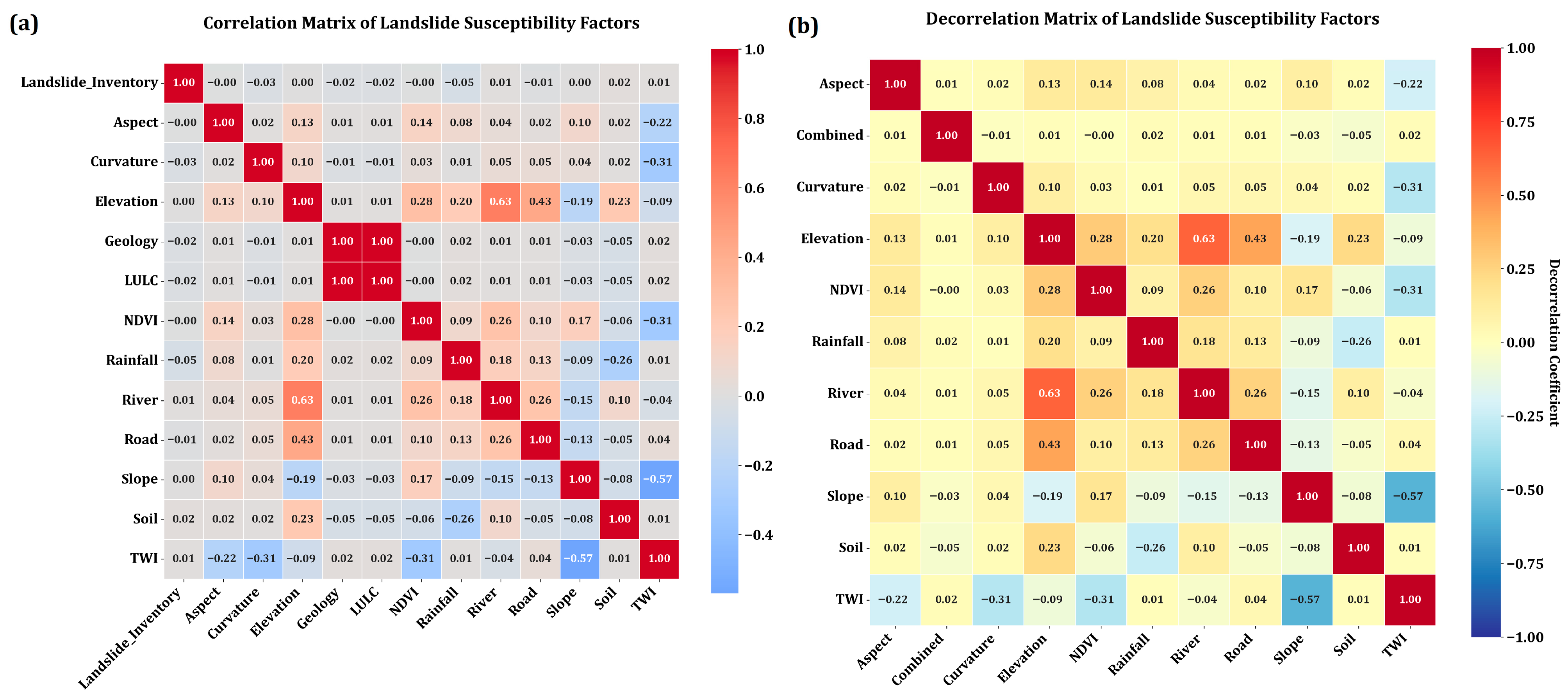
The collinearity matrix reveals key relationships between the predictive factors (Figure 4a). Distance to river and elevation show a strong positive correlation (r = 0.631), while both variables correlate negatively with slope and TWI (approximately r = −0.570). A primary concern is the perfect positive correlation between geology and LULC (r = 1.0), which necessitated the use of PCA to address this multicollinearity.
NDVI demonstrates a moderate positive correlation with elevation (r = 0.284) and a moderate negative correlation with TWI (r = −0.314), suggesting a potential vegetation stabilization effect. Distance to road correlates strongly with elevation (r = 0.432). In contrast, aspect, curvature, and soil show negligible correlations with other factors.
The perfect correlation (r = 1) between geology and LULC stems from spatial data limitations on the regional scale. Analysis revealed a complete overlap where soft rock areas consistently correspond with agricultural land, while hard rock formations aligned exclusively with forest cover. This categorical overlap created statistical multicollinearity despite the variables representing distinct conceptual domains. PCA resolution maintained both factors’ contributions while eliminating redundancy.

3.1.2. PCA Application

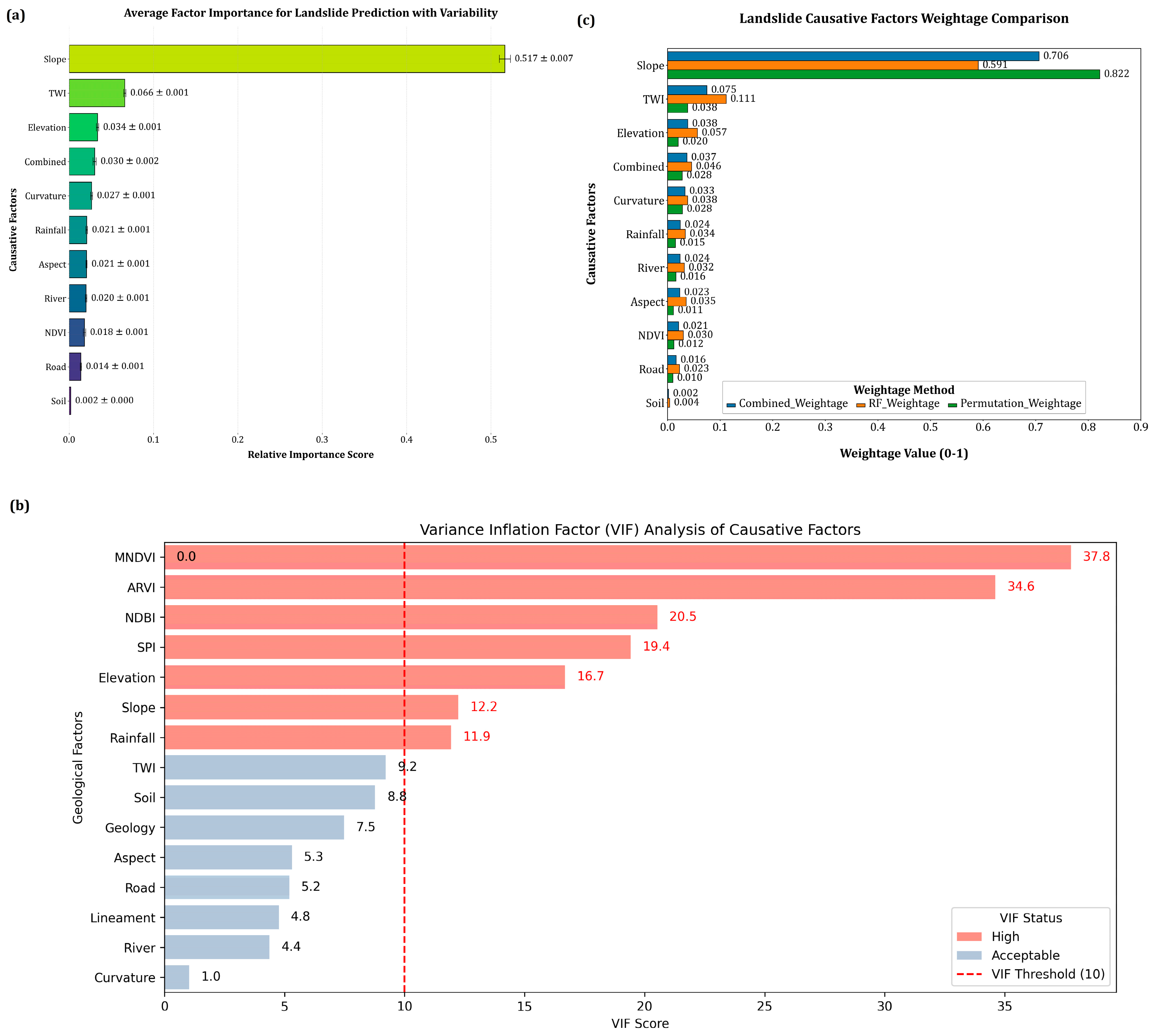
Principal Component Analysis (PCA) successfully resolved the multicollinearity between geology and LULC by combining them into a single, major composite factor (Figure 4b). This new factor was geomorphologically meaningful and eliminated redundancy, as confirmed by the Variance Inflation Factor (VIF) values below 5 for all variables (Figure 5b). The Distance to Road (VIF = 0.634) and Distance to River (VIF = 0.572) showed acceptable multicollinearity levels. The PCA-derived composite factor exhibited the highest VIF value of 1.004, which remains well below the critical threshold. Conversely, curvature (VIF = 0.010) and NDVI (VIF = 0.028) demonstrated very low multicollinearity, indicating their independent predictive strength.

3.1.3. Factor Importance Assessment

Slope was the most influential factor, demonstrating high importance in both the Random Forest (0.59) and Permutation (0.44) methods, with low variability (SD = 0.01). The Topographic Wetness Index (TWI) was the second most important factor (average importance = 0.07) but showed a notable discrepancy between the Random Forest (0.11) and Permutation (0.02) results, suggesting a contextual dependency. In contrast, elevation, curvature, and rainfall made consistently low contributions (average = 0.02–0.03, SD = 0.00). The soil factor was found to be non-significant (0.19) and was therefore excluded from the final model (Figure 5a). The complete results are provided in Table A2.
The final weighting scheme allocates 50% of the importance to the dominant factor, slope, 7% to TWI, and 23% or less to secondary factors (Figure 5c and Table 1). This distribution achieves a balance between statistical rigor and geomorphological plausibility, offering an improvement over a subjective expert-based approach. The minimal weight assigned to anthropogenic variables, such as distance to road, underscores the predominant control of natural terrain characteristics in this Himalayan context. All causative factors showed stable weights, as indicated by modest standard deviations (≤0.01).
Factor ranking confirms slope as the dominant predictor with a combined weight of 70.63, demonstrating high consistency between the Random Forest (59.08) and Permutation (82.18) methods. TWI ranks second (7.48) but exhibits a notable discrepancy between methods (11.14 vs. 3.82), suggesting its influence is context dependent. Lower-ranked factors: elevation, curvature, and rainfall contribute minimally (less than 5% combined). The soil factor was negligible (0.19) and was excluded from the final model (Figure 5c and Table 1).
Based on these results, three distinct landslide susceptibility models using a weighted-overlay approach were developed. Each employs a different importance-weighting scheme. The Random Forest-weighted model applied the weight values from Table 1 to assess landslide susceptibility through factor overlay analysis using Equations (21) and (23) [46].
L S I = 0.591 × Slope   + 0.111 × T W I + i 3 10   w i × F i
Similarly, the Permutation-Weighted model using Equations (21) and (24) [46] utilized the weight values from Table 1 to evaluate landslide susceptibility through factor overlay analysis.
L S I = 0.822 × Slope   + 0.038 × T W I + i = 3 10   w i × F i
Furthermore, using weights from Table 1, the Combined Weight Model using Equations (21) and (24) [46] assessed landslide susceptibility via factor overlay analysis.
L S I = 0.706 × Slope   + 0.075 × T W I + i = 3 10   w i × F i

3.2. Comparative Analysis of Landslide Susceptibility Models

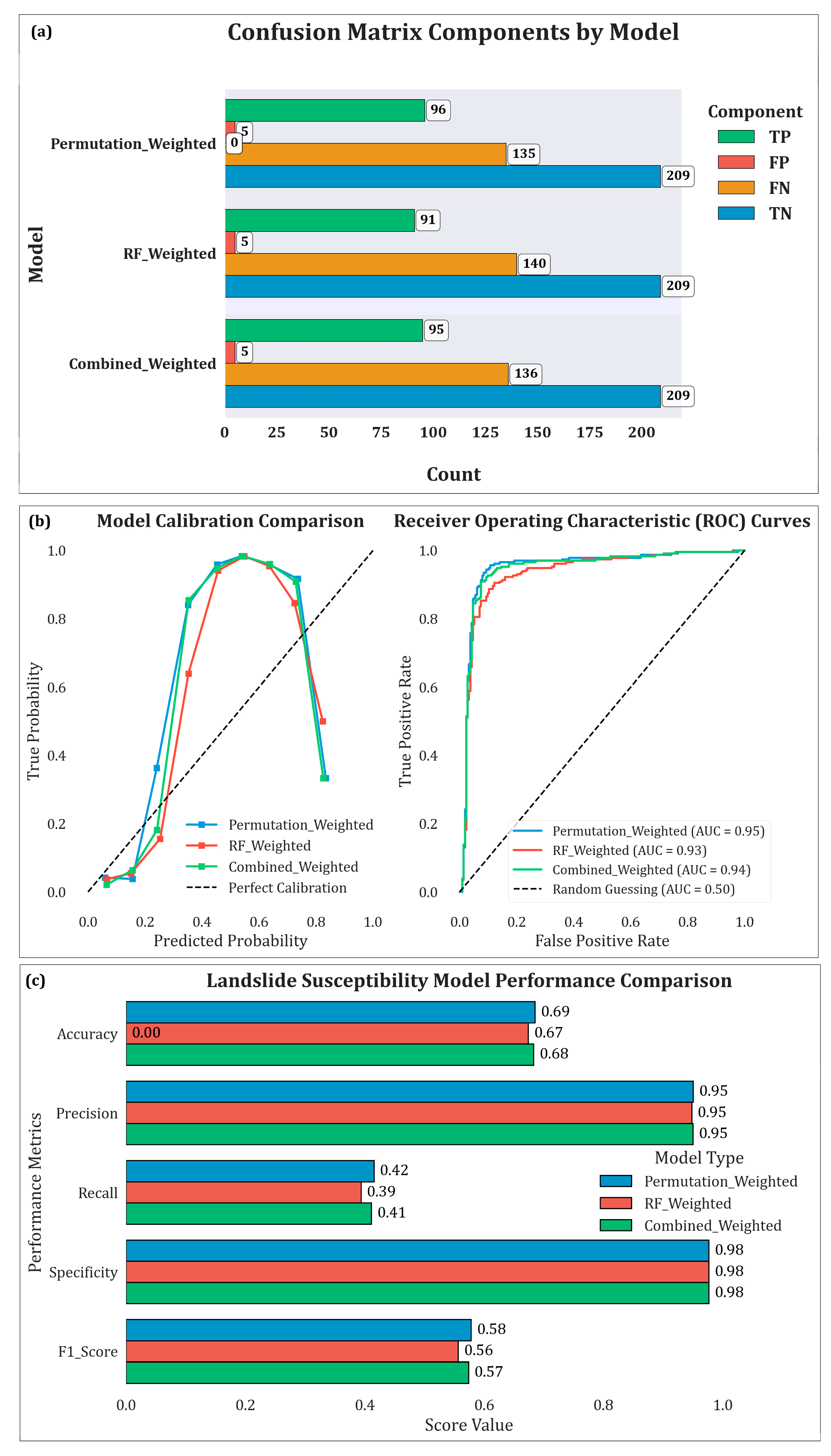
Statistical measures confirm the superior performance of the Permutation-Weighted model over the Combined and Random Forest (RF) models for landslide risk assessment. The Permutation model achieved the best metrics, including 69% accuracy, 66% recall, 95% precision, and an excellent AUC of 95% (Figure 6b). It also attained the highest F1-score of 78%, indicating a better balance between precision and recall than the alternative models (77% and 76%).
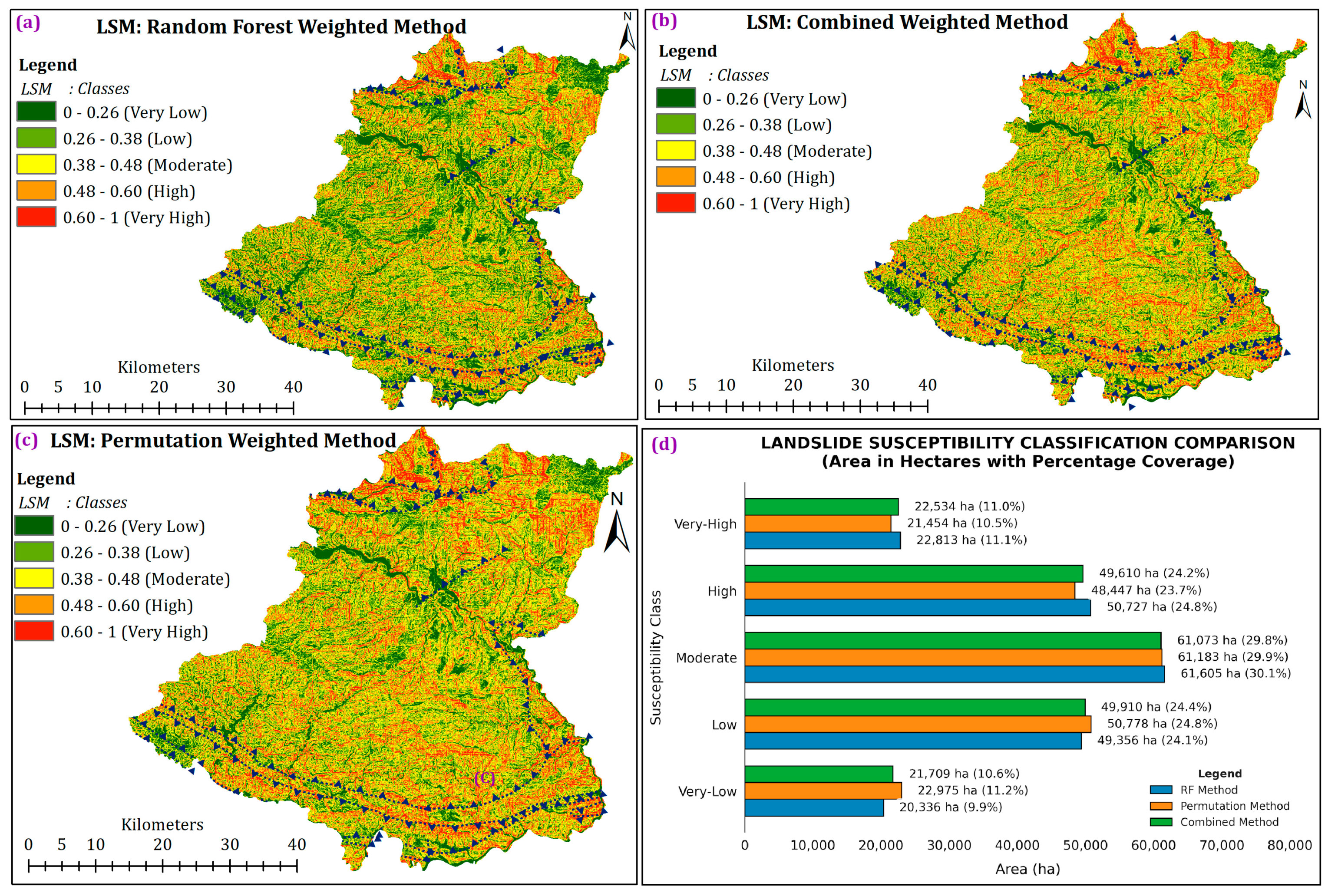
The landslide susceptibility maps (LSMs) generated using Random Forest (RF), Permutation, and Combined Weighting Methods offer crucial insights for both theoretical outcomes and practical applications of landslide risk management. All three methods show consistent distribution frequencies, classifying 30.1% of the study area as Moderate susceptibility, 26.7% as Low, and 24.5% as High-risk (Figure 6c). The techniques demonstrate strong agreement in identifying susceptibility thresholds, with minimal variation (≤3%) in the allocation of the Moderate class. The Permutation method shows greater sensitivity to extreme risks, assigning 18.3% of the area to the Very-Low class and 12.4% to the Very-High class. In contrast, the RF method is more conservative, distributing 15.2% to Very-Low and 7.2% to Very-High areas. The Combined method provides a consensus outcome with moderate distributions of 16.7% (Very Low) and 9.8% (Very High), reflecting a balanced result. Overall, the three techniques show strong agreement, identifying 35.2–36.9% of the study region as combined High and Very-High risk areas, with 10–12% classified as Very-High risk. These high-risk zones require immediate attention for effective hazard management.
The consistent identification of transitional (Moderate) susceptibility zones across all methods (±0.3% variation) is highly valuable for development planning (Figure 6c). While the weighting strategies produce different distributions near class boundaries, with the Permutation method showing 5–7% greater distinction between extreme classes than RF, all methods successfully identify the primary spatial risk patterns. The Combined approach synthesizes the strengths of the individual methods by maintaining the integrity of the total high-risk area (36.1%). This synthesis of RFs’ moderate performance and Permutations’ sensitivity to extremes makes the combined model the most suitable option for operational landslide control (Figure 6c). From multicollinearity testing to weight derivation, this methodology produces interpretable and statistically validated susceptibility results, with less than 3% deviation between models. These results can directly inform mitigation efforts in Very-High Zones, land-use regulations in Moderate-risk areas, and slope-based early warning systems.

3.3. Accuracy Assessment and Model Performance Evaluation

Statistical measures confirm the superior performance of the Permutation-Weighted model over the Combined and Random Forest (RF) models for landslide risk assessment. The Permutation model achieved the best metrics, including 69% accuracy, 66% recall, 95% precision, and an excellent AUC of 95% (Figure 7b). It also attained the highest F1-score of 78%, indicating a better balance between precision and recall than the alternative models (77% and 76%).
While the Combined model demonstrated a twice higher landslide detection rate in very high-risk areas than the RF model (Figure 7c), the Permutation model’s higher recall rate proves more effective at identifying actual landslide locations. This higher recall, combined with its consistent performance across all evaluation metrics, makes the Permutation model particularly suitable for landslide risk assessment. Its robust performance enables both precise hazard zonation and practical risk management applications.
A comprehensive comparison of model performance metrics (Table 2) demonstrates the clear superiority of the Permutation-Weighted approach, which achieved the highest scores across all evaluation criteria (AUC: 0.95 ± 0.01, F1-score: 0.78 ± 0.02) with minimal variance. While the Random Forest model showed strong precision (0.90 ± 0.02), its lower recall (0.60 ± 0.04) limited its overall effectiveness, and the Combined method provided intermediate but consistently inferior results compared to the Permutation-Weighted model.

3.4. Verification of Landslide Risk Assessment Outcomes

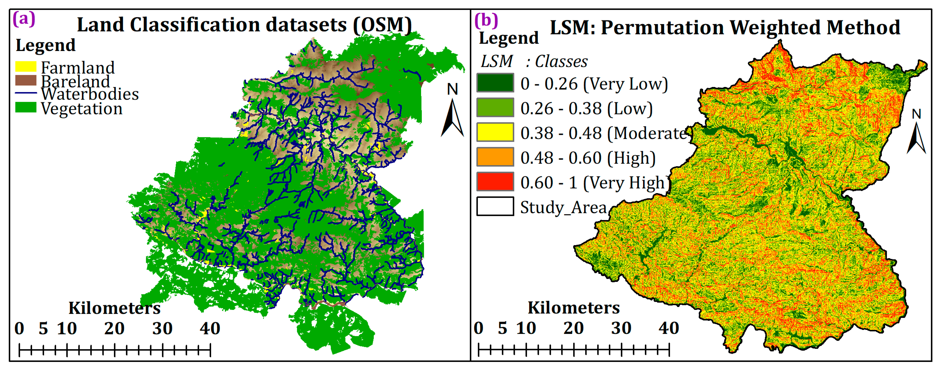
The Permutation-Weighted model outclassed in LSMs generation with AUC: 95% and accuracy: 69%, which validated its selection for this operation while OpenStreetMap exposure layers remained essential (Figure 8a,b).
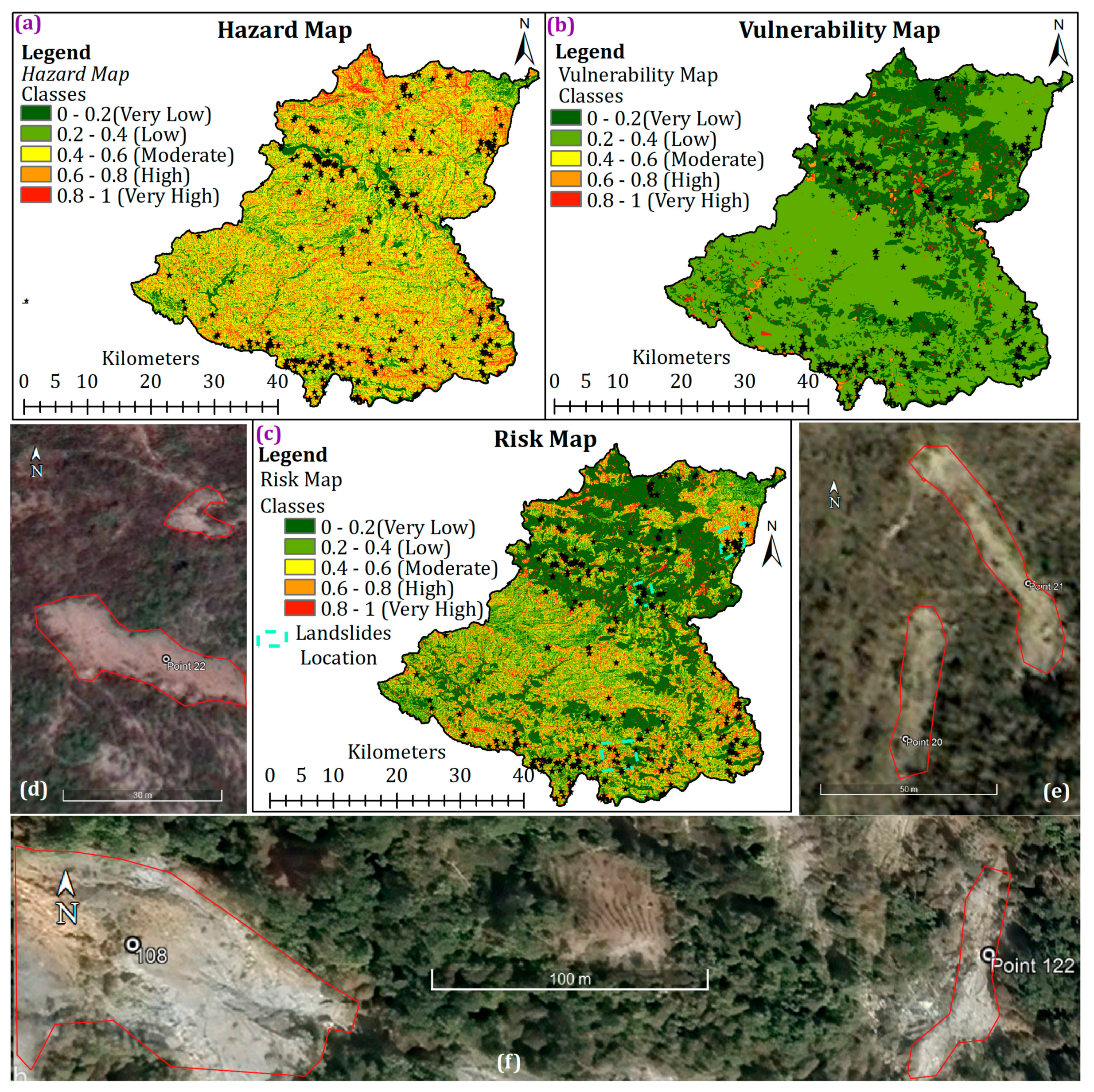
Finally, the study generated three fundamental outputs (Hazard, Vulnerability and Risk Map) for landslide risk assessment that were divided further into five categories through natural breaks classification method: Very Low (0–0.2) and Low (0.2–0.4) and Moderate (0.4–0.6) and High (0.6–0.8) and Very High (0.8–1) (Figure 9a–c). The locations of the previously recorded landslides are marked by black stars on all maps (Figure 9a–c). The predicted high-risk areas from the risk map were verified with ground truth using Google Earth imagery, showing in blue polygons (Figure 9d–f) that match well with the actual landslide locations shown in Figure 9d–f. Additionally, the final landslide risk map depicts Very High-risk areas while providing actionable protection information obtained through analyzing risk areas. Hence, the predictive method adopted demonstrated accurate forecasting capabilities, confirming its reliability as a suitable model for landslide risk areas.

4. Discussion

This study provides an integrated framework for landslide susceptibility mapping that addresses both methodological challenges and regional specificities of the Far-Western region of Nepal. The analysis confirms slope as the dominant controlling factor (51.7% contribution), which reflects fundamental geomorphological processes in the Himalayan context [60]. Steep slopes (>25°) developed on Doti Schist formations exhibit shallow soil depths and reduced shear strength [61], particularly when combined with high-intensity monsoon rainfall that increases pore pressure [62]. These slopes primarily correspond with tectonic features, including the Main Central Thrust zone, where ongoing uplift creates over-steepened terrain with structurally weak planes [63]. The parallel high weighting of TWI further confirms the role of hydrological convergence in slope saturation [62,63], creating critical failure conditions at specific topographic positions. This integrated perspective demonstrates how topographic, lithological, and hydrological factors interact to control landslide distribution patterns [61,63], revealing greater topographic dominance in Doti compared to other regions with more complex geology.
The successful resolution of perfect multicollinearity between geology and LULC through PCA represents a key methodological improvement [16,64], particularly relevant for Himalayan landscapes where these factors are intrinsically linked. When contextualized with similar studies, the model proposed demonstrates competitive performance. The Permutation-Weighted model’s superior discrimination capacity (AUC = 95%) exceeds values reported for other Himalayan regions [12,65], while the moderate accuracy (69%) reflects expected performance trade-offs in complex terrain [66]. This performance pattern underscores the importance of our feature selection approach while highlighting persistent challenges in regional LSM [15].
Computational efficiency was evaluated during model development, with the Random Forest algorithm completing training in approximately 45 min on a standard workstation (Intel i7 processor, 16 GB RAM), demonstrating the framework’s practicality for regional applications. The permutation importance calculations, while computationally intensive, provided crucial insights into feature significance without substantially impacting the overall workflow efficiency.
This study systematically addresses three uncertainty sources: (1) Data uncertainty from inventory completeness and regional-scale geological mapping [23,25]; (2) Parameter uncertainty in RF hyperparameters and classification thresholds [5,6]; (3) Spatial uncertainty evidenced by 11% of historical landslides outside predicted high-risk zones [67,68]. These limitations highlight the need for careful interpretation of model outputs [69].
The framework’s scalability to other geomorphological settings appears promising, given its reliance on globally available data sources and standardized processing techniques. Future applications could test its adaptability in diverse Himalayan sub-regions and potentially other mountain environments with similar landslide mechanisms, though this would require validation against local inventory data and potentially the incorporation of region-specific triggering factors. This statistically validated framework provides a replicable approach for landslide risk assessment in data-scarce Himalayan environments, while explicitly acknowledging uncertainties to guide appropriate application in land-use planning and disaster risk reduction. Moreover, while this study employed standard random splitting for model validation, future work could benefit from spatial cross-validation techniques to better account for spatial autocorrelation and improve model generalizability across different geographical subsets.

5. Conclusions

This study presents a new framework for landslide susceptibility assessment that systematically addresses three primary challenges: predictor multicollinearity, subjective weighting, and incomplete risk assessment. Through PCA and VIF analysis, the approach successfully resolved multicollinearity between geology and LULC factors, achieving an optimal VIF of 1.004. The analysis identified slope as the dominant controlling factor (50–70% contribution), followed by TWI (7%).
The Permutation-Weighted model demonstrated superior predictive capability with an AUC of 95%, accuracy of 69%, and recall of 66%, while the combined weighting approach proved most valuable for risk mitigation planning. Spatial validation confirmed 89% agreement between predicted High/Very High-risk zones (covering 35% of the study area) and historical landslide records.
While the methodological framework shows strong potential for application in data-deficient regions, its transferability to other geographical contexts requires careful consideration. Key limitations for cross-regional application include (1) variations in geological settings and dominant triggering mechanisms, (2) differences in data quality and availability, and (3) region-specific landslide characteristics. Successful implementation in new areas would require recalibration using local landslide inventories and conditioning factors.
The framework provides valuable insights for disaster management authorities in the Nepal Himalayas, particularly for infrastructure planning in high-risk zones. Future research should focus on incorporating temporal rainfall dynamics and enhanced anthropogenic factors to address climate change impacts and land-use pressures. With proper localization, this approach holds significant promise for implementation in other geologically active regions facing similar landslide challenges.

Author Contributions

B.R.J. performed all aspects of the research, including data collection, preparation, and management; methodological development; landslide susceptibility mapping and analysis; and manuscript drafting. N.K. and C.B. contributed to model validation, data quality control, results verification, and manuscript refinement. The contributions of I.P.A. included intellectual refinement of the study concept and scholarly revision of the manuscript with constructive feedback. N.P.B. provided supervisory oversight, guided manuscript revisions, and approved the final version. All authors have read and agreed to the published version of the manuscript.

Funding

This research received no external funding.

Informed Consent Statement

Informed consent was obtained from all subjects involved in the study.

Data Availability Statement

The data used in this study can be accessed through ASTER DEM and Landsat 8 datasets, in addition to receiving the other causative factors that incorporate road layers, soil components, LULC, Buildings, bare land, Settlements, geology, lineament, and stream components.

Acknowledgments

The completion of this study is due to the funding, materials, and resources provided by the Japan Society of Promotion of Science (JSPS Japan), Ehime University, Japan, and Pokhara University, Nepal. The data extracted from Google Earth, SOTER Database for Nepal, the Department of Geology and Mines of Nepal, CHIRPS (Climate Hazards Group Infrared Precipitation Station), and the European Space Agency, which provided ASTER DEM and Landsat 8 datasets, are also sincerely acknowledged. Authors acknowledge AI-assisted technologies for English language editing, grammar checking, and text paraphrasing during the preparation of this manuscript.

Conflicts of Interest

The authors declare no conflicts of interest.

Appendix A

Table A1. Weight of Evidence (WoE) analysis for categorical factors (geology, soil types, LULC) showing class statistics, information values (IV), normalized weights, and label encoding ranks.
SNLCFClass No.ClassClass Pixels Count% Class Pixels (a)Landslide Pixels Count% Landslide in Class (b)IV = ln(b/a)Normalized WeightageLabel Encoding
1Geology1Ba20950.0009198680000.59652853510
2Basic Rocks58,70000.2577387492420.217625899−0.1691689390.54743495112
3Bu146,8420.064475082820.0737410070.1342802230.6354972576
4Damgad Formation105,5660.0463517012070.1861510791.39030059811
5Galyang Formation39,6340.017402415210.0188848920.0817532560.6202536968
6Gh5710.0002507140000.59652853510
7Gn15,9980.00702436910.000899281−2.05554556017
8Granites130,0800.057115258110.009892086−1.7533362190.08770250516
9Lakharpata Formation48,6820.021375192440.0395683450.6157984360.7752360014
10Melmura Formation74,0790.032526454300.026978417−0.1870165550.54225549213
11Ranimatta Formation245,9220.1079789241240.1115107910.0321853070.6058688559
12Sallyani Gad Formation606,2470.266189682780.070143885−1.3336605130.20949427614
13Sangram Formation10,9200.00479473160.0053956830.1180816530.630796367
14Siwalik46,4390.02039034330.0296762590.3752860920.7054382415
15Suntar Formation56,9220.024993194550.0494604320.682569430.7946132433
16Swat Formation88290.00387661910.000899281−1.4611236040.17250391615
17Syangja Formation151,6740.0665967071770.1591726620.8713344060.8493936852
2,277,500 1112
2Soil types1CMe1,603,0430.7038608128350.7508992810.0646909020.6562165823
2CMg17,3260.00760746470.006294964−0.189379960.5438353655
3Cmo17650.00077497320.0017985610.84191464411
4CMu44,6090.01958682810.00089928100.6276023514
5CMx483,9210.2124790341720.154676259−0.3175090390.4871610126
6RGd84,5170.03710955900.0809352520.7797751270.9725143042
7RGe42,3190.01858133950.004496403−1.41888009107
2,277,500 1112
3LULC types1Agricultural Land269,4220.1182972561580.1420863310.1832342640.1118409336
2Bareland44,0150.019326015410.0368705040.6459597360.3942752734
3Builtup Area98,9530.0434480791360.1223021581.034928050.6316903623
4Forests1,373,2350.602957193140.282374101007
5Grassland451,6090.1982915483840.3453237410.5547439460.3385997745
6Riverbed15,9180.006989243400.0359712231.63834706411
7Waterbody24,3480.01069067390.0350719421.188030090.7251394512
2,277,500 1112
Table A2. Factor importance statistics derived from Permutation, Random Forest, and Average Weighting methods.
Causative FactorsRandom Forest_ImportancePermutation ImportanceStd_Dev.Average Importance
Slope0.590.440.010.52
TWI0.110.0200.07
Elevation0.060.0100.03
Combined0.050.0100.03
Curvature0.040.0200.03
Rainfall0.030.0100.02
Aspect0.040.0100.02
Distance to River0.030.0100.02
NDVI0.030.0100.02
Distance to Road0.020.0100.01
Soil0000

References

  1. Petley, D. Global Patterns of Loss of Life from Landslides. Geology 2012, 40, 927–930. [Google Scholar] [CrossRef]
  2. Froude, M.J.; Petley, D.N. Global Fatal Landslide Occurrence from 2004 to 2016. Nat. Hazards Earth Syst. Sci. 2018, 18, 2161–2181. [Google Scholar] [CrossRef]
  3. Kargel, J.S.; Leonard, G.J.; Shugar, D.H.; Haritashya, U.K.; Bevington, A.; Fielding, E.J.; Young, N. Geomorphic and Geologic Controls of Geohazards Induced by Nepal’s 2015 Gorkha Earthquake. Science 2016, 351, aac8353. [Google Scholar] [CrossRef] [PubMed]
  4. Lamichhane, K.; Biswakarma, K.; Acharya, B.; Karki, S.; KC, R.; Subedi, M.; Sharma, K. Preliminary Assessment of September 2024 Extreme Rainfall–Induced Landslides in Central Nepal. Landslides 2025, 22, 3281–3295. [Google Scholar] [CrossRef]
  5. Gariano, S.L.; Guzzetti, F. Landslides in a Changing Climate. Earth Sci. Rev. 2016, 162, 227–252. [Google Scholar] [CrossRef]
  6. Haque, U.; Blum, P.; Da Silva, P.F.; Andersen, P.; Pilz, J.; Chalov, S.R.; Keellings, D. Fatal Landslides in Europe. Landslides 2016, 13, 1545–1554. [Google Scholar] [CrossRef]
  7. Deuba, T. More than 250 Families Displaced by Landslides in Doti. The Himalayan Times. 2015. Available online: https://thehimalayantimes.com/nepal/more-than-250-families-displaced-by-landslides-in-doti/ (accessed on 8 October 2025).
  8. Deuba, T. Haliya Settlement at Risk in Doti. The Himalayan Times. 2018. Available online: https://thehimalayantimes.com/nepal/haliya-settlement-at-risk-in-doti (accessed on 10 October 2025).
  9. RSS. Landslide Displaces Eight Families in Doti. Ratopati. 2020. Available online: https://english.ratopati.com/story/13941 (accessed on 10 October 2025).
  10. Deuba, T. Landslide Obstructs Bhimdutta Highway in Sudurpaschim. The Himalayan Times. 2021. Available online: https://thehimalayantimes.com/nepal/landslide-obstructs-bhimdutta-highway-in-sudurpaschim (accessed on 10 October 2025).
  11. Bist, D.B.; Thapa, M.S.; Bista, U.; Awasthi, N. Analytical Hierarchy Process (AHP) Based Landslide Susceptibility Mapping of Kaligandaki Hydro-Catchment of Syangja, Nepal. Available online: Agric. For. J. 2020, 4, 80–90. [Google Scholar]
  12. Regmi, A.D.; Devkota, K.C.; Yoshida, K.; Pradhan, B.; Pourghasemi, H.R.; Kumamoto, T.; Akgun, A. Application of Frequency Ratio, Statistical Index, and Weights-of-Evidence Models and Their Comparison in Landslide Susceptibility Mapping in Central Nepal Himalaya. Arab. J. Geosci. 2014, 7, 725–742. [Google Scholar] [CrossRef]
  13. Polykretis, C.; Chalkias, C. Comparison and Evaluation of Landslide Susceptibility Maps Obtained from Weight of Evidence, Logistic Regression, and Artificial Neural Network Models. Nat. Hazards 2018, 93, 249–274. [Google Scholar] [CrossRef]
  14. Pham, B.T.; Prakash, I.; Singh, S.K.; Shirzadi, A.; Shahabi, H.; Tran, T.T.T.; Bui, D.T. Landslide Susceptibility Modeling Using Reduced Error Pruning Trees and Different Ensemble Techniques: Hybrid Machine Learning Approaches. Catena 2019, 175, 203–218. [Google Scholar] [CrossRef]
  15. Merghadi, A.; Yunus, A.P.; Dou, J.; Whiteley, J.; ThaiPham, B.; Bui, D.T.; Abderrahmane, B. Machine Learning Methods for Landslide Susceptibility Studies: A Comparative Overview of Algorithm Performance. Earth-Sci. Rev. 2020, 207, 103225. [Google Scholar] [CrossRef]
  16. Pandey, V.K.; Pourghasemi, H.R.; Sharma, M.C. Landslide Susceptibility Mapping Using Maximum Entropy and Support Vector Machine Models along the Highway Corridor, Garhwal Himalaya. Geocarto Int. 2020, 35, 168–187. [Google Scholar] [CrossRef]
  17. Mandal, B.; Mondal, S.; Mandal, S. GIS-Based Landslide Susceptibility Zonation (LSZ) Mapping of Darjeeling Himalaya, India Using Weights of Evidence (WoE) Model. Arab. J. Geosci. 2023, 16, 421. [Google Scholar] [CrossRef]
  18. Aboutaib, F.; Krimissa, S.; Pradhan, B.; Elaloui, A.; Ismaili, M.; Abdelrahman, K.; Namous, M. Evaluating the Effectiveness and Robustness of Machine Learning Models with Varied Geo-Environmental Factors for Determining Vulnerability to Water Flow-Induced Gully Erosion. Front. Environ. Sci. 2023, 11, 1207027. [Google Scholar] [CrossRef]
  19. Feizizadeh, B.; Blaschke, T. GIS-Multicriteria Decision Analysis for Landslide Susceptibility Mapping: Comparing Three Methods for the Urmia Lake Basin, Iran. Nat. Hazards 2013, 65, 2105–2128. [Google Scholar] [CrossRef]
  20. Pourghasemi, H.R.; Rossi, M. Landslide Susceptibility Modeling in a Landslide Prone Area in Mazandarn Province, North of Iran: A Comparison between GLM, GAM, MARS, and M-AHP Methods. Theor. Appl. Climatol. 2017, 130, 609–633. [Google Scholar] [CrossRef]
  21. Kappes, M.S.; Papathoma-Köhle, M.; Keiler, M. Assessing Physical Vulnerability for Multi-Hazards Using an Indicator-Based Methodology. Appl. Geogr. 2012, 32, 577–590. [Google Scholar] [CrossRef]
  22. Glade, T. Vulnerability Assessment in Landslide Risk Analysis. Erde 2003, 134, 123–146. [Google Scholar]
  23. Saba, S.B.; van der Meijde, M.; van der Werff, H. Spatiotemporal Landslide Detection for the 2005 Kashmir Earthquake Region. Geomorphology 2010, 124, 17–25. [Google Scholar] [CrossRef]
  24. Wei, X.; Zhang, L.; Gardoni, P.; Chen, Y.; Tan, L.; Liu, D.; Li, H. Comparison of Hybrid Data-Driven and Physical Models for Landslide Susceptibility Mapping at Regional Scales. Acta Geotech. 2023, 18, 4453–4476. [Google Scholar] [CrossRef]
  25. Steger, S.; Brenning, A.; Bell, R.; Glade, T. The Influence of Systematically Incomplete Shallow Landslide Inventories on Statistical Susceptibility Models and Suggestions for Improvements. Landslides 2017, 14, 1767–1781. [Google Scholar] [CrossRef]
  26. Zhang, W.; Li, H.; Li, Y.; Liu, H.; Chen, Y.; Ding, X. Application of Deep Learning Algorithms in Geotechnical Engineering: A Short Critical Review. Artif. Intell. Rev. 2021, 54, 5633–5673. [Google Scholar] [CrossRef]
  27. Wang, Y.; Wang, L.; Liu, S.; Han, L.; Zhang, W.; Hong, L.; Zhu, X. Region Similarity Assessment for Empowering Physics-Informed Transfer Learning-Based Landslide Susceptibility Mapping. J. Rock Mech. Geotech. Eng. 2025, in press. [CrossRef]
  28. Cui, H.Z.; Tong, B.; Wang, T.; Dou, J.; Ji, J. A Hybrid Data-Driven Approach for Rainfall-Induced Landslide Susceptibility Mapping: Physically Based Probabilistic Model with Convolutional Neural Network. J. Rock Mech. Geotech. Eng. 2024, 17, 4933–4951. [Google Scholar] [CrossRef]
  29. Wang, Y.H.; Wang, L.Q.; Zhang, W.G.; Liu, S.L.; Sun, W.X.; Hong, L.; Zhu, Z.W. A Physics-Informed Machine Learning Solution for Landslide Susceptibility Mapping Based on Three-Dimensional Slope Stability Evaluation. J. Cent. South Univ. 2024, 31, 3838–3853. [Google Scholar] [CrossRef]
  30. Wang, Y.; Wang, L.; Liu, S.; Liu, P.; Zhu, Z.; Zhang, W. A Comparative Study of Regional Landslide Susceptibility Mapping with Multiple Machine Learning Models. Geol. J. 2024, 59, 2383–2400. [Google Scholar] [CrossRef]
  31. Singh, A.; Dhiman, N.; KC, N.; Shukla, D.P. Improving ML-Based Landslide Susceptibility Using Ensemble Method for Sample Selection: A Case Study of Kangra District in Himachal Pradesh, India. Environ. Sci. Pollut. Res. 2024, 31, 1–24. [Google Scholar] [CrossRef] [PubMed]
  32. Singh, A.; Dhiman, N.; Niraj, K.C.; Shukla, D.P. Ensembled Transfer Learning Approach for Error Reduction in Landslide Susceptibility Mapping of the Data Scare Region. Sci. Rep. 2024, 14, 29060. [Google Scholar] [CrossRef]
  33. Kincey, M.E.; Rosser, N.J.; Swirad, Z.M.; Robinson, T.R.; Shrestha, R.; Pujara, D.S.; Basyal, G.K.; Densmore, M.E.; Arrell, K.; Oven, K.J.; et al. National-Scale Rainfall-Triggered Landslide Susceptibility and Exposure in Nepal. Earth’s Future 2024, 12, e2023EF004102. [Google Scholar] [CrossRef]
  34. Niraj, K.C.; Singh, A.; Shukla, D.P. Effect of the Normalized Difference Vegetation Index (NDVI) on GIS-Enabled Bivariate and Multivariate Statistical Models for Landslide Susceptibility Mapping. J. Indian Soc. Remote Sens. 2023, 51, 1739–1756. [Google Scholar] [CrossRef]
  35. Hayashi, D. Geological Reconnaissance around Silgarhi-Doti, West Central Nepal. Bull. Coll. Sci. Univ. Ryukyus 1984, 38, 103–116. [Google Scholar]
  36. Tiwari, R.K.; Paudyal, H. Spatial Mapping of b-Value and Fractal Dimension Prior to November 8, 2022, Doti Earthquake, Nepal. PLoS ONE 2023, 18, e0289673. [Google Scholar] [CrossRef] [PubMed]
  37. Bhandari, G. Trends in Seasonal Precipitation and Temperature–A Review in Doti and Surkhet Districts of Nepal. Int. J. Environ. 2013, 2, 269–279. [Google Scholar] [CrossRef]
  38. Paudyal, N.; Khadka, R.B.; Khadka, R. Agricultural Perspectives of Climate Change Induced Disasters in Doti, Nepal. J. Agric. Environ. 2013, 14, 149–159. [Google Scholar] [CrossRef]
  39. Wagle, N.; Acharya, T.D.; Kolluru, V.; Huang, H.; Lee, D.H. Multi-Temporal Land Cover Change Mapping Using Google Earth Engine and Ensemble Learning Methods. Appl. Sci. 2020, 10, 8083. [Google Scholar] [CrossRef]
  40. Chao, Z.; Gan, L.; Cao, Y.; Wang, Y.; Segoni, S.; Shi, X.; Motagh, M.; Singh, R.P. Landslide Susceptibility Assessment of the Wanzhou District: Merging Landslide Susceptibility Modelling (LSM) with InSAR-Derived Ground Deformation Map. Int. J. Appl. Earth Obs. Geoinf. 2025, 136, 104365. [Google Scholar] [CrossRef]
  41. Phuyal, B.; Thapa, P.B.; Devkota, K.C. Characterization of Large-Scale Landslides and Their Susceptibility Evaluation in Central Nepal Himalaya. J. Nepal Geol. Soc. 2022, 63, 109–122. [Google Scholar] [CrossRef]
  42. Zighmi, K.; Zahri, F.; Faqeih, K.; Al Amri, A.; Riheb, H.; Alamri, S.M.; Alamery, E. AHP Multi Criteria Analysis for Landslide Susceptibility Mapping in the Tellian Atlas Chain. Sci. Rep. 2025, 15, 25747. [Google Scholar] [CrossRef]
  43. Ali, P.J.M.; Faraj, R.H.; Koya, E. Data Normalization and Standardization: A Technical Report. Mach. Learn. Tech. Rep. 2014, 1, 1–6. [Google Scholar]
  44. Asuero, A.G.; Sayago, A.; González, A.G. The Correlation Coefficient: An Overview. Crit. Rev. Anal. Chem. 2006, 36, 41–59. [Google Scholar] [CrossRef]
  45. Dormann, C.F.; Elith, J.; Bacher, S.; Buchmann, C.; Carl, G.; Carré, G.; Lautenbach, S. Collinearity: A Review of Methods to Deal with It and a Simulation Study Evaluating Their Performance. Ecography 2013, 36, 27–46. [Google Scholar] [CrossRef]
  46. Parhizkar, T.; Rafieipour, E.; Parhizkar, A. Evaluation and Improvement of Energy Consumption Prediction Models Using Principal Component Analysis Based Feature Reduction. J. Clean. Prod. 2021, 279, 123866. [Google Scholar] [CrossRef]
  47. Dou, J.; Yunus, A.P.; Bui, D.T.; Merghadi, A.; Sahana, M.; Zhu, Z.; Chen, C.-W.; Khosravi, K.; Yang, Y.; Pham, B.T. Assessment of Advanced Random Forest and Decision Tree Algorithms for Modeling Rainfall-Induced Landslide Susceptibility in the Izu-Oshima Volcanic Island, Japan. Sci. Total Environ. 2019, 662, 332–346. [Google Scholar] [CrossRef]
  48. Xia, D.; Tang, H.; Sun, S.; Tang, C.; Zhang, B. Landslide Susceptibility Mapping Based on the Germinal Center Optimization Algorithm and Support Vector Classification. Remote Sens. 2022, 14, 2707. [Google Scholar] [CrossRef]
  49. Wang, H.; Yang, F.; Luo, Z. An Experimental Study of the Intrinsic Stability of Random Forest Variable Importance Measures. BMC Bioinform. 2016, 17, 60. [Google Scholar] [CrossRef]
  50. Altmann, A.; Toloşi, L.; Sander, O.; Lengauer, T. Permutation Importance: A Corrected Feature Importance Measure. Bioinformatics 2010, 26, 1340–1347. [Google Scholar] [CrossRef]
  51. Newey, W.K.; Stoker, T.M. Efficiency of Weighted Average Derivative Estimators and Index Models. Econometrica 1993, 61, 1199–1223. [Google Scholar] [CrossRef]
  52. Fawcett, T. An Introduction to ROC Analysis. Pattern Recognit. Lett. 2006, 27, 861–874. [Google Scholar] [CrossRef]
  53. Huang, F.; Cao, Z.; Guo, J.; Jiang, S.-H.; Li, S.; Guo, Z. Comparisons of Heuristic, General Statistical and Machine Learning Models for Landslide Susceptibility Prediction and Mapping. Catena 2020, 191, 104580. [Google Scholar] [CrossRef]
  54. Koks, E.E.; Jongman, B.; Husby, T.G.; Botzen, W.J. Combining Hazard, Exposure, and Social Vulnerability to Provide Lessons for Flood Risk Management. Environ. Sci. Policy 2015, 47, 42–52. [Google Scholar] [CrossRef]
  55. Abdiweli, A.J. Simulation Study on the Performance of Robust Outlier Labelling Methods. Ph.D. Thesis, Kampala International University, Kampala, Uganda, October 2023. Available online: https://irbackend.kiu.ac.ug/server/api/core/bitstreams/86d8fd79-e3c5-408a-98f1-48de5057c608/content (accessed on 10 October 2025).
  56. Ma, S.; Shao, X.; Xu, C. Delineating Non-Susceptible Landslide Areas in China Based on Topographic Index and Quantile Non-Linear Model. Forests 2024, 15, 678. [Google Scholar] [CrossRef]
  57. Wannous, C.; Velasquez, G. United Nations Office for Disaster Risk Reduction (UNISDR)—UNISDR’s Contribution to Science and Technology for Disaster Risk Reduction and the Role of the International Consortium on Landslides (ICL). In Advancing Culture of Living with Landslides: Volume 1 ISDR-ICL Sendai Partnerships 2015–2025; Sassa, K., Mikos, M., Yin, Y., Eds.; Springer: Cham, Switzerland, 2017; pp. 109–115. [Google Scholar] [CrossRef]
  58. Maini, R.; Clarke, L.; Blanchard, K.; Murray, V. The Sendai Framework for Disaster Risk Reduction and Its Indicators—Where Does Health Fit In? Int. J. Disaster Risk Sci. 2017, 8, 150–155. [Google Scholar] [CrossRef]
  59. Michael, E.A.; Samanta, S. Landslide Vulnerability Mapping (LVM) Using Weighted Linear Combination (WLC) Model through Remote Sensing and GIS Techniques. Model. Earth Syst. Environ. 2016, 2, 88. [Google Scholar] [CrossRef]
  60. Devkota, K.C.; Regmi, A.D.; Pourghasemi, H.R.; Yoshida, K.; Pradhan, B.; Ryu, I.C.; Althuwaynee, O.F. Landslide Susceptibility Mapping Using Certainty Factor, Index of Entropy and Logistic Regression Models in GIS and Their Comparison at Mugling–Narayanghat Road Section in Nepal Himalaya. Nat. Hazards 2013, 65, 135–165. [Google Scholar] [CrossRef]
  61. Das, S.; Pandit, K.; Sarkar, S.; Kanungo, D.P. Stability and Hazard Assessment of the Progressive Zero Landslide in the Kalimpong Region of Darjeeling Himalaya, India. Geotech. Geol. Eng. 2024, 42, 1693–1709. [Google Scholar] [CrossRef]
  62. Okalp, K.; Akgün, H. Assessing Landslide Susceptibility of Türkiye at Drainage Basin Scale: A Semi-Quantitative Approach. Nat. Hazards 2025, 121, 20099–20127. [Google Scholar] [CrossRef]
  63. Zeraatpisheh, M.; Ayoubi, S.; Sulieman, M.; Rodrigo-Comino, J. Determining the Spatial Distribution of Soil Properties Using the Environmental Covariates and Multivariate Statistical Analysis: A Case Study in Semi-Arid Regions of Iran. J. Arid Land 2019, 11, 551–566. [Google Scholar] [CrossRef]
  64. Chen, W.; Pourghasemi, H.R.; Kornejady, A.; Zhang, N. Landslide Spatial Modeling: Introducing New Ensembles of ANN, MaxEnt, and SVM Machine Learning Techniques. Geoderma 2017, 305, 314–327. [Google Scholar] [CrossRef]
  65. Wang, H.; Zhang, L.; Yin, K.; Luo, H.; Li, J. Landslide Identification Using Machine Learning. Geosci. Front. 2021, 12, 351–364. [Google Scholar] [CrossRef]
  66. Reichenbach, P.; Rossi, M.; Malamud, B.D.; Mihir, M.; Guzzetti, F. A Review of Statistically-Based Landslide Susceptibility Models. Earth-Sci. Rev. 2018, 180, 60–91. [Google Scholar] [CrossRef]
  67. Hong, H.; Liu, J.; Bui, D.T.; Pradhan, B.; Acharya, T.D.; Pham, B.T.; Ahmad, B.B. Landslide Susceptibility Mapping Using J48 Decision Tree with AdaBoost, Bagging and Rotation Forest Ensembles in the Guangchang Area (China). Catena 2018, 163, 399–413. [Google Scholar] [CrossRef]
  68. Frattini, P.; Crosta, G.; Carrara, A. Techniques for Evaluating the Performance of Landslide Susceptibility Models. Eng. Geol. 2010, 111, 62–72. [Google Scholar] [CrossRef]
  69. Huang, F.; Cao, Z.; Jiang, S.-H.; Zhou, C.; Huang, J.; Guo, Z. Landslide Susceptibility Prediction Based on a Semi-Supervised Multiple-Layer Perceptron Model. Landslides 2020, 17, 2919–2930. [Google Scholar] [CrossRef]
Figure 1. Study area map and visual evidence of four significant landslides in the area: (a) location of Nepal in South Asia, (b) detailed topographic view of Doti District (Study Area) with the landslide locations, and (c) landslide scenario in the study area (location is indicated in (b)).
Applsci 15 12152 g001
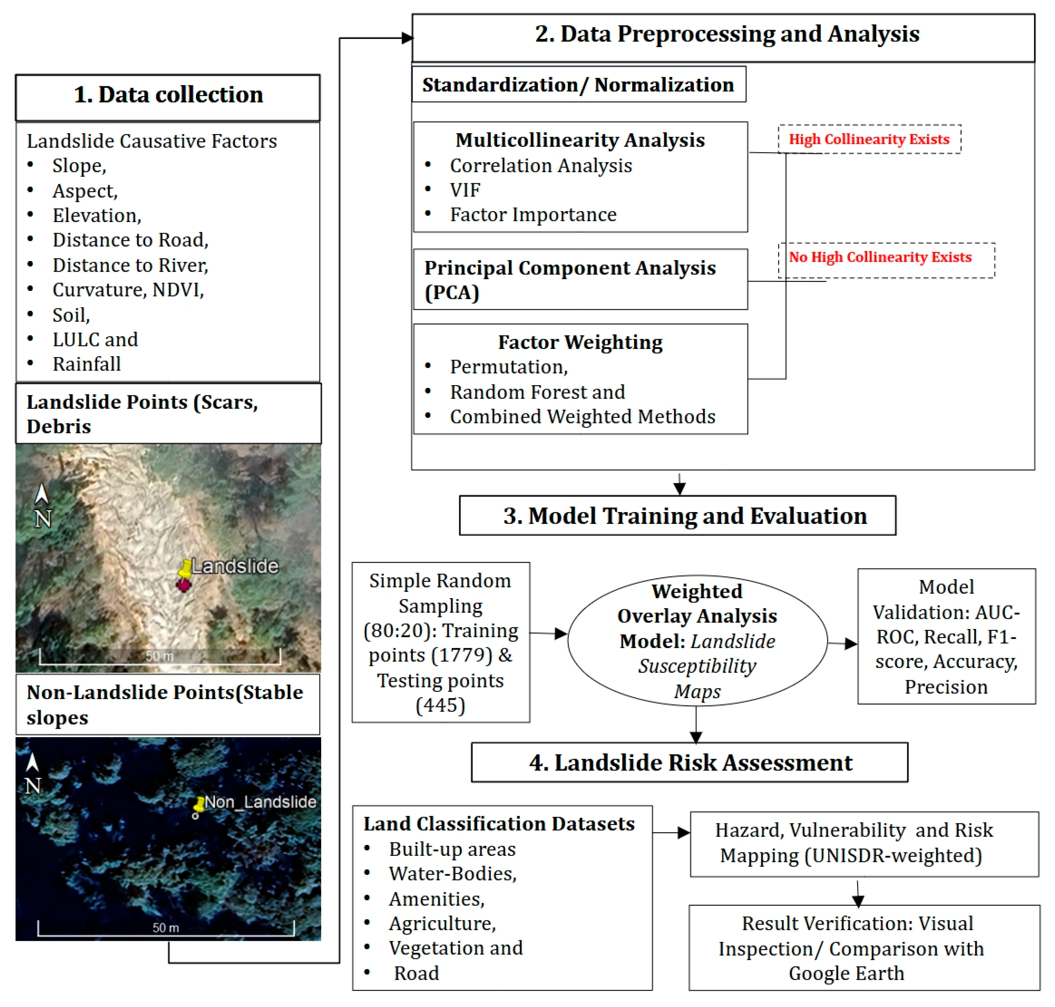
Figure 2. Methodological framework adopted in this study, indicating the procedure of landslide inventory, causative factor processing, followed by model integration, susceptibility mapping, and risk assessment.
Applsci 15 12152 g002
Figure 3. Spatial distribution of landslide causative factors: (a) aspect, (b) curvature, (c) elevation, (d) slope, (e) topographic wetness index (TWI), (f) distance to river, (g) land use land cover (LULC), (h) distance to road, (i) normalized difference vegetation index (NDVI), (j) soil, (k) rainfall, and (l) geology; mapped at 30 m resolution (WGS 1984, UTM Zone 44N).
Applsci 15 12152 g003
Figure 4. Multicollinearity assessment of conditioning factors: (a) Pearson correlation matrix, and (b) PCA-based factor decorrelation for landslide susceptibility mapping.
Applsci 15 12152 g004
Figure 5. Multicollinearity analysis and factor weighting: (a) factor importance ranking, (b) VIF-based multicollinearity assessment (where factors colored red have a VIF score greater than the threshold of 10, indicating severe multicollinearity), and (c) comparison of RF, permutation, and combined weighting methods.
Applsci 15 12152 g005
Figure 6. LSMs generated using (a) Random Forest, (b) Combined weighting, and (c) Permutation weighting methods; (d) compares the area of all LSMs in hectares.
Applsci 15 12152 g006
Figure 7. Statistical metrics and performance evaluation of LSM models, highlighting the accuracy and reliability of each weighting method: (a) Confusion Matrix Components, (b) Model Calibration Comparison and ROC Curves, and (c) Landslide Susceptibility Model Performance Comparison.
Applsci 15 12152 g007
Figure 8. (a) Vulnerability and exposure variables across the study area, and (b) Superior LSM generated using the Permutation-Weighted method for landslide risk assessment.
Applsci 15 12152 g008
Figure 9. (a) Hazard, (b) Vulnerability, and (c) Risk maps. Very High-Risk zones in the Risk map (c) are validated with Google Earth imagery (df). The actual spatial extent of historical landslides is clearly delineated with red polygons in validation images (df), demonstrating strong alignment with the predicted high-risk zones in (c).
Applsci 15 12152 g009
Table 1. Weight allocation for landslide causative factors across different modeling approaches.
RankLandslide Causative FactorsCombined WeightageRandom Forest WeightagePermutation Weightage
1Slope0.70640.59070.8218
2TWI0.07480.11140.0382
3Elevation0.03840.05670.0201
4Combined0.03670.04570.0278
5Curvature0.03320.03810.0283
6Rainfall0.02430.03370.0149
7Distance to River0.02380.03180.0158
8Aspect0.02320.03540.0111
9NDVI0.0210.03010.012
10Distance to Road0.01630.02260.01
11Soil0.00190.00390
Table 2. Comparative performance of the landslide susceptibility models.
ModelAUC (±Std)Accuracy (±Std)Precision (±Std)Recall (±Std)F1-Score (±Std)
Random Forest0.92 (±0.02)0.65 (±0.03)0.90 (±0.02)0.60 (±0.04)0.72 (±0.03)
Permutation-Weighted0.95 (±0.01)0.69 (±0.02)0.95 (±0.01)0.66 (±0.03)0.78 (±0.02)
Combined0.93 (±0.02)0.67 (±0.02)0.92 (±0.02)0.63 (±0.03)0.75 (±0.02)
Disclaimer/Publisher’s Note: The statements, opinions and data contained in all publications are solely those of the individual author(s) and contributor(s) and not of MDPI and/or the editor(s). MDPI and/or the editor(s) disclaim responsibility for any injury to people or property resulting from any ideas, methods, instructions or products referred to in the content.