Hybrid Deep Learning Framework for Damage Detection in Urban Railway Bridges Based on Linear Variable Differential Transformer Data

Abstract

Urban railway bridges are critical components of modern transportation networks. Dynamic loads and harsh environments put urban railway bridges at high risk of damage. Conventional vibration-based damage detection approaches often fail to provide sufficient accuracy and robustness under complex urban conditions. To address this limitation, this study introduces a hybrid deep learning framework that integrates a one-dimensional convolutional neural network (1D-CNN) and a recurrent neural network (RNN) for automatic damage detection using Linear Variable Differential Transformer (LVDT) displacement data. Start with the calibration of a finite element model (FEM) of the target bridge, achieved through updating the model parameters to align with field-acquired LVDT data, thereby establishing a robust and reliable baseline representation of the structure’s behaviour. Subsequently, a series of failure and damage scenarios is introduced within the FEM, and the associated dynamic displacement responses are generated to construct a comprehensive synthetic training dataset. These time-series responses serve as input for training a hybrid deep learning architecture, which integrates a one-dimensional convolutional neural network (1D-CNN) for automated feature extraction with a recurrent neural network (RNN) designed to capture the temporal dependencies inherent in the structural response data. Results show rapid convergence and minimal error in single-damage cases, and robust performance in multi-damage conditions on a dataset exceeding 5 million samples; the model attains a mean absolute error of ≈3.2% for damage severity and an average localisation error of <0.7 m. The findings highlight the effectiveness of combining numerical simulation with advanced data-driven approaches to provide a practical, data-efficient, and scalable solution for structural health monitoring in the urban railway context.

1. Introduction

Urban railway systems are essential elements in completing the transport infrastructure of large cities. The development of urban railway systems contributes to reducing the load on main routes, limiting traffic jams, and ensuring people’s movement. Urban railway bridges are a crucial component of urban railway lines. Over time, these bridge structures are subjected to various dynamic loads from train operations, environmental impacts, and material degradation, leading to the risk of damage. It reduces their integrity and operational capacity. Faced with this problem, timely and accurate detection of structural damage is essential.

Structural Health Monitoring (SHM) systems have received considerable attention in recent years [1,2,3]. The achievements of SHM bring significant benefits. In particular, SHM systems significantly increase the service life of structures by providing early warnings, thereby supporting management units in the maintenance process. Modern SHM systems often integrate many sensors, data processing, and analysis modules [4,5]. The task of the sensors is to collect changes in the structure, such as temperature, strain, stress, vibration, or displacement [6,7,8]. The signals, after being collected, will be transmitted to the processing unit for analysis and evaluation [9]. This cycle takes place continuously to ensure comprehensive monitoring of the structure.

One of the most important tasks in the field of SHM is damage detection. It is also the task that has received the most research attention to improve further and develop the SHM system. Damage detection methods based on dynamic signals have been of interest to researchers and have been strongly developed. Traditional methods often rely on modal parameters such as natural frequencies, modal shapes, and damping ratios to infer structural damage [10,11,12]. These methods have been widely applied and have achieved certain successes. Saidin et al. [13] utilised the concept that the stiffness index ratio alters the structural response to vibration. Based on this, the study proposed a solution to detect structural damage in ultra-high-performance concrete bridges. He and Zhu [14] have proposed the basic theories and applications for utilising natural frequency variation to detect structural damage. Gillich et al. [15] proposed using frequency shift to detect structural damage in beams. In addition, many other studies have also applied vibration data to detect structural damage [16,17,18,19]. However, after a long period of use, people have begun to realise some limitations. These solutions are very sensitive to environmental and operational changes. Additionally, the ability to locate damage under actual load conditions remains limited [20,21].

Displacement is one of the factors closely related to stiffness degradation (elastic modulus and geometric characteristics of the structure). Unlike vibration characteristics, displacement provides a more direct interpretation of structural performance. Additionally, displacement factors are more intuitive than vibration. The measured displacement is a physical quantity that is intuitive and easy to calibrate [22]. It is less affected by environmental noise than vibration acceleration signals. With a reasonable arrangement of displacement measurement points, it is possible to both monitor the global deformation of the structure and detect local damage at a specific location [23,24]. Among the existing sensor technologies, Linear Variable Differential Transformer (LVDT) sensors have been shown to be very effective in capturing dynamic displacements with high resolution and low noise. Displacement-based methods, particularly those utilising LVDT sensors, are emerging as a more efficient and reliable approach in structural health monitoring. Compared to traditional vibration methods, it provides a signal that is more sensitive to damage, is easier to collect, and can be easily integrated into modern machine learning systems for the purpose of automatic damage detection and localisation.

The 4.0 industrial revolution, with the remarkable development of artificial intelligence (AI), is creating a breakthrough in the field of SHM, in general, and the potential in structural damage detection in particular [25]. AI is applied in research to enhance the effectiveness of SHM systems. Several studies have been conducted on the application of AI in structural damage detection. Nguyen and Livaoğlu [26] proposed and developed a damage detection method for structures using artificial neural networks, achieving accurate results for the considered cases. Viet et al. [27] improved the accuracy of structural damage detection by using an ANN combined with swarm intelligence. Ruffels et al. [28] trained an ANN to detect damage in a steel arch bridge model in the laboratory. The study demonstrated the effectiveness of ANN in detecting structural damage in various scenarios [29].

In recent years, deep learning models have emerged strongly due to their superior capabilities compared to traditional ANN networks [30,31]. Convolutional Neural Networks (CNNs) have been widely applied to vibration signals and strain data to extract spatial features relevant to damage [32,33,34]. Teng et al. [25] extracted damage features from the bridge population using a CNN, and then the trained CNN was used to detect bridge structural damage. Xue et al. [35] proposed the use of a one-dimensional convolutional neural network (1D-CNN) for the automatic detection of structural damage. The findings demonstrated that the proposed method proved to be both effective and highly accurate.

On the other hand, Recurrent Neural Networks (RNNs) have demonstrated superior performance in modelling temporal dependencies in sequential data [36]. Based on this advantage, Sahoo and Jena [37] used an RNN to detect damage to the Hybrid Composite Beam. Dang et al. [38] applied an RNN in detecting structural damage using time series data. However, individual application of CNNs or RNNs may not fully capture both the localised damage-sensitive patterns and the sequential characteristics of structural responses.

In recent years, research on deep-learning-based SHM has evolved rapidly, with a growing emphasis on hybrid architectures and diverse sensing modalities. Deep learning has become a powerful tool for structural health monitoring (SHM), enabling data-driven identification of damage patterns from sensor signals. Fu et al. [39] combined CNN and LSTM networks for damage identification of long-span bridges. Das and Guchhait [40] developed a structural damage detection method using GRU-LSTM using time domain acceleration data. These recent advances underscore the trend toward hybrid deep learning frameworks that combine spatial and temporal feature extraction while leveraging richer sensing data. Nevertheless, most existing studies continue to rely on acceleration or strain measurements, with limited exploration of LVDT displacement data, which can directly capture localised deformation [41]. This gap highlights the need for further investigation into displacement-driven, hybrid deep learning models—such as the one proposed in this study—for accurate and robust bridge damage detection in complex urban environments.

However, most existing studies rely on vibration or acceleration signals and focus on single-model architectures such as CNN or LSTM, which may fail to capture both spatial and temporal dependencies effectively. Moreover, few works have explored the potential of LVDT displacement data for bridge damage detection, despite its high sensitivity to localised structural changes. These limitations motivate the development of a hybrid deep learning approach that can fully exploit displacement information for more accurate and robust damage assessment.

This study proposes a novel damage detection methodology for urban railway bridges based on dynamic displacement data collected from LVDT sensors. By combining a One-Dimensional Convolutional Neural Network (1D CNN) with a Recurrent Neural Network (RNN), the proposed approach leverages the strengths of both architectures to learn spatial-temporal features from raw displacement signals. The methodology is validated through a case study on the Cat Linh–Ha Dong urban railway line in Hanoi, Vietnam, where dynamic displacement data were collected under actual train load conditions. The results demonstrate the effectiveness of the hybrid 1DCNN-RNN model in accurately identifying damage severity and localising damage areas on the bridge structure. This research contributes to the field of structural health monitoring by introducing an integrated data-driven framework capable of processing high-resolution displacement data for real-time damage assessment of urban railway bridges.

The novelty of the present study consists of three key aspects: (i) the integration of LVDT displacement data, which directly captures structural deformation with higher sensitivity to stiffness degradation; (ii) the use of an FEM-updated digital twin to generate a large-scale synthetic training dataset representing multiple damage scenarios; (iii) the continuous prediction of both damage severity and location, rather than discrete classification. These innovations provide a physically grounded, data-efficient, and scalable approach that distinguishes this study from previous works.

2. Methodology

2.1. Using LVDT Data for Damage Detection

The dynamic behaviour of a bridge structure can be represented by the following second-order differential equation in matrix form:

$$M\ddot{u}(t)+C\dot{u}(t)+Ku(t)=F(t)$$

(1)

where $\mathrm{M}\in {\mathrm{R}}^{\mathrm{n}\times \mathrm{n}}$: mass matrix; $\mathrm{C}\in {\mathrm{R}}^{\mathrm{n}\times \mathrm{n}}$: damping matrix; $\mathrm{K}\in {\mathrm{R}}^{\mathrm{n}\times \mathrm{n}}$: stiffness matrix; $\mathrm{u}(t)\in {\mathrm{R}}^{\mathrm{n}\times 1}$: displacement vector at time $t$; $\mathrm{F}(t)\in {\mathrm{R}}^{\mathrm{n}\times 1}$: external force vector.

Damage in the structure leads to a change in the stiffness matrix:

$$K_d=K- \Delta K$$

(2)

where $K_d$: stiffness matrix of the damaged structure; $\Delta K$: reduction in stiffness due to damage.

The displacement response under the same external load changes accordingly:

$$u_d(t)=K_d^{-1}F(t)\approx K_d^{-1}F(t)+K^{-1}\Delta K{K}^{-1}F(t)$$

(3)

The approximate displacement difference due to damage is:

$$u(t)=u_d(t)-u(t)\approx -K^{-1}\Delta Ku(t)$$

(4)

This expression shows that the change in displacement is directly proportional to the damage-induced stiffness reduction and the original displacement.

Assume that LVDT sensors are placed at selected degrees of freedom, forming an observation vector $y(t)$

$$y(t)=Hu(t)$$

(5)

where $\mathrm{y}(t)\in {\mathrm{R}}^{\mathrm{m}\times 1}$: LVDT measurements; $\mathrm{H}\in {\mathrm{R}}^{\mathrm{m}\times \mathrm{n}}$: observation matrix selecting the displacement components corresponding to the sensor locations; $\mathrm{m}$: number of LVDT sensors.

The damaged observation becomes:

$$y_d(t)=H{u}_d(t)$$

(6)

The change in observation due to damage:

$$\Delta y(t)=y_d(t)-y(t)\approx H\Delta u(t)\approx -H{K}^{-1}\Delta Ku(t)$$

(7)

It indicates that the LVDT response variation contains embedded information about the location and severity of the damage through the term $\Delta K$.

In this study, the observation model assumes a linear mapping $H$ that includes not only the selection of structural DOFs but also the interpolation from FE nodes to the actual sensor positions and the projection along the LVDT measurement axes. Each LVDT was mounted on the girder soffit and referenced to a ground-anchored frame, thus measuring the absolute vertical deflection of the girder rather than rail motion. Constant offsets were zeroed during field calibration, and slow drifts were removed by detrending. Since the sensors were not attached to the rail, rail–structure interaction effects enter only through the loading model and do not appear explicitly in $y(t)$.

Although Equations (1)–(7) are written in the form of a linearised dynamic equilibrium, they are introduced merely to describe the general relationship between nodal forces and displacements. In practice, the underlying finite-element model and the synthetic dataset generation include material and geometric nonlinearities (e.g., stiffness degradation, contact effects, and large deflection). Therefore, the proposed learning framework does not rely on linear elasticity; instead, it learns the nonlinear mapping between measured displacement responses and the corresponding damage states. The linear form is used only as a first-order descriptor to maintain analytical clarity and comparability with standard SHM formulations.

Bridge responses may involve nonlinearities due to material softening, contact and separation, or hysteretic damping. These effects were implicitly included in the synthetic dataset generated from the updated finite element model and are captured by the data-driven learning process of the hybrid CNN–RNN framework. The proposed method is not limited to linear–elastic behaviour but can accommodate nonlinear structural responses through data representation.

The present formulation is intended for structural conditions within the serviceability and moderate-damage range, where deformations are small and the overall stiffness-displacement relationship can be approximated by a linearised model. In such cases, the linear dynamic equilibrium serves as a reference, whereas the neural network learns deviations from this baseline, effectively representing higher-order, amplitude-dependent responses. While severe nonlinear phenomena such as contact, separation, and hysteretic energy dissipation are beyond the scope of this study, they can be incorporated in future work through nonlinear finite-element simulations or hybrid physics-informed networks that explicitly model hysteresis and evolving boundary conditions.

2.2. One-Dimensional Convolutional Neural Network (1D CNN)

One-dimensional Convolutional Neural Networks (1D CNNs) are a powerful class of deep learning models that automatically extract local and hierarchical features from time-series data. In this study, the LVDT displacement responses $y(t)$ are treated as one-dimensional time series, where the convolution operation captures both spatial and temporal patterns, as well as sudden changes in displacement caused by structural damage. The input to a 1D CNN layer is a sequence $\mathrm{X}\in {\mathrm{R}}^{\mathrm{T}\times \mathrm{c}}$), where $\mathrm{T}$ is the length of the time series window and $c$ is the number of input channels (in this case, the number of LVDT sensors).

The 1D convolutional operation is mathematically expressed as:

$$z_k^{(l)}(t)=\sum _{i=1}^{c_l-1}\sum _{j=1}^K{w}_{k,i,j}^{(l)}.x_i^{(l-1)}(t+j-1)+b_k^{(l)}$$

(8)

where

• $z_k^{(l)}(t)$: output feature at position $t$ and channel $k$ in layer $l$
• $w_{k,i,j}^{(l)}$: kernel weight connecting input channel $i$ to output channel $k$, with kernel size $K$
• $b_k^{(l)}$: bias term for output channel $k$
• $x_i^{(l-1)}(t)$: input from the previous layer (or raw data if $l=1$),
• $c_{l-1}$: number of channels in the previous layer

The convolutional layer is typically followed by a nonlinear activation function $\sigma$, such as the Rectified Linear Unit (ReLU):

$$a_k^{(l)}(t)=\sigma (z_k^{(l)}(t))=\mathit{max}(0,z_k^{(l)}(t))$$

(9)

To reduce dimensionality and control overfitting, a pooling layer follows the convolution:

$$p_k^{(l)}(t)=\mathit{max}(a_k^{(l)}(t),a_k^{(l)}(t+1),\dots ,a_k^{(l)}(t+P-1))$$

(10)

where $P$ is the pooling size, pooling enables the network to retain the most prominent features while reducing the number of parameters and computational requirements.

The output of the CNN feature extractor is denoted as $h_{CNN}\in {\mathrm{R}}^{\mathrm{d}}$ where $d$ is the total number of extracted features.

2.3. Recurrent Neural Network (RNN)

RNNs are specifically designed for analysing sequential data, where the temporal correlation between data points plays a crucial role. In the context of structural damage detection, the displacement responses measured by LVDT sensors are time-dependent signals. After local feature extraction by the 1D CNN, the RNN is employed to model long-term dependencies and temporal evolution patterns that may indicate damage progression or sudden structural changes.

The RNN processes the output feature sequence from the CNN module, denoted as $h_{CNN}(t)$, where $t$ is the time step.

The basic operation of a vanilla RNN cell at time step $t$ is formulated as:

$$h_t=\varphi (W_{xh}{x}_t+W_{hh}{h}_{t-1}+b_h)$$

(11)

$$y_t=W_{hy}{h}_t+b_y$$

(12)

where $x_t\in {\mathrm{R}}^{\mathrm{d}}$: input feature vector at time step $t$ (output from CNN); $h_t\in {\mathrm{R}}^{\mathrm{d}}$: hidden state vector at time $t$; $y_t\in {\mathrm{R}}^{\mathrm{o}}$: output vector; $W_{xh}\in {\mathrm{R}}^{\mathrm{h}\times \mathrm{d}}$, $W_{hh}\in {\mathrm{R}}^{\mathrm{h}\times \mathrm{d}}$, $W_{hy}\in {\mathrm{R}}^{\mathrm{o}\times \mathrm{h}}$: weight matrices; $b_h$, $b_y$: bias vectors; $\varphi (.)$: activation function, typically tanh or ReLU.

The final hidden state, $h_T$, after processing all time steps, serves as a compressed representation of the temporal dynamics of the displacement sequence. This state is passed through a fully connected (dense) layer with a softmax or sigmoid activation to classify the damage state:

$$\widehat{y}=Softmax(W_{hq}{h}_T+b_q)$$

(13)

where $\widehat{y}$ is the predicted probability distribution over the possible damage states.

2.4. Hybrid 1DCNN-RNN for Damage Detection Using LVDT Data

While 1DCNN efficiently extracts local spatial patterns from LVDT displacement time series, it cannot model temporal dependencies and long-term behaviour changes indicative of structural damage evolution. Conversely, RNNs are designed to capture temporal correlations but may struggle with raw, unprocessed data due to noise and irrelevant features. Therefore, this study proposes a hybrid 1DCNN-RNN architecture that combines the strengths of both models. The 1D CNN extracts damage-sensitive features from raw displacement measurements. The RNN captures temporal patterns and dependencies, enabling the model to learn the progression and characteristics of structural damage over time. 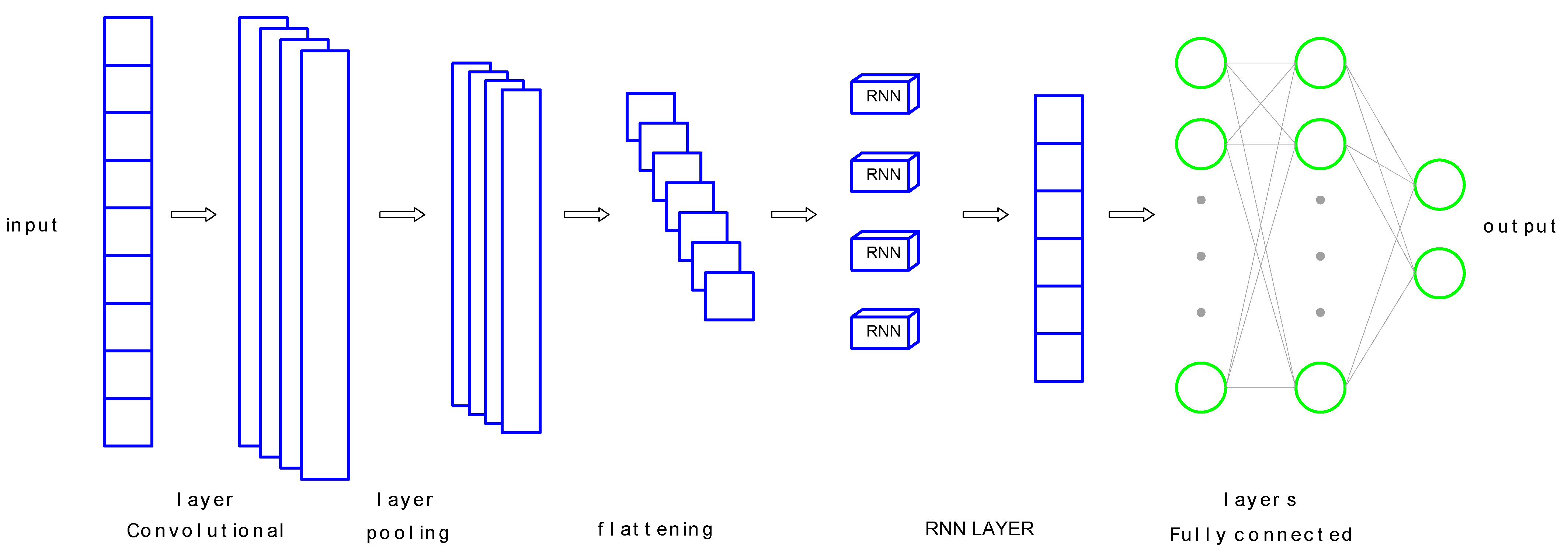Figure 1 presents the proposed framework in this study.

The model’s input is the time-series displacement measured from LVDT sensors placed at multiple locations on the bridge structure. First, convolutional layers (1DCNN) extract local features in the displacement signal, which helps detect abnormal fluctuations due to structural damage. Subsequent pooling layers reduce the dimensionality of the data and retain important features. After the feature extraction step, the data is converted to one-dimensional vectors through the flattening process and then fed into RNN layers to learn features in a time sequence. RNN is responsible for identifying long-term changes and abnormal trends in the structure’s response. The network’s output consists of two main values: damage percentage and damage location. This process not only allows for the detection of damage presence or absence but also enables the assessment of damage severity and specific location within the structure. The combination of CNN’s local feature extraction capability and RNN’s time-dependent learning capability improves the accuracy and reliability in structural health monitoring using LVDT data.

In this study, the dataset was generated based on scenarios simulated from the updated finite element (FE) model. However, it is recognised that numerical simulations inherently contain several sources of uncertainty that may affect the accuracy and representativeness of the generated data. These uncertainties originate from variations in material properties, assumptions in boundary conditions, mesh discretisation, and measurement noise in the LVDT signals used for model calibration. To mitigate their influence, stochastic perturbations were introduced during data generation to improve the robustness of the deep learning model and to prevent overfitting to idealised numerical conditions. Although these strategies reduce the effects of modelling uncertainties, further experimental validation and probabilistic assessment are recommended to enhance the overall reliability of the proposed framework.

The influence of initialisation strategies and modelling assumptions on the simulation and learning outcomes was also considered. In the FE model, variations in boundary constraints and initial stiffness distributions were examined to verify that the updated model remained stable and representative of realistic bridge behaviour. For the deep learning framework, random initialisation of network weights and data shuffling were repeated over multiple runs to confirm the consistency of results. The performance metrics reported in this study, therefore, represent the average of repeated experiments, minimising the potential bias caused by initialisation randomness or minor modelling assumptions. This approach ensures that the conclusions drawn are robust and not overly dependent on specific initialisation settings.

3. Case Study

3.1. Data Gathering

In this study, a monitoring campaign was undertaken to collect dynamic displacement data from urban railway bridges. The selected case study was the Cat Linh-Ha Dong urban railway bridge in Hanoi, Vietnam (Figure 2). The Cat Linh-Ha Dong line is an urban railway system linking Cat Linh with Ha Dong, with a total length of 13,021.48 m. Its superstructure consists of a series of simple supported spans with box-section girders. The span lengths vary between 18.5 and 32 m.

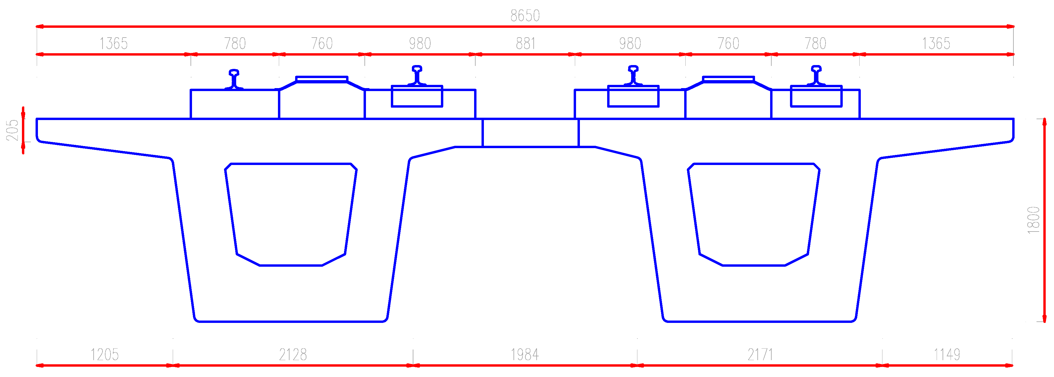
The selected segment for data collection is a simple span located near Yen Nghia station, with the permission of the Hanoi Urban Railway Management Board. The bridge span structure for data collection is a 32 m span type. The cross-section of the girder is box-shaped. The girder cross-section is constant (Figure 3), with a total height of 1800 mm. The width of the girder is 3950 mm. The longest cantilever of the bridge deck, according to the design, is 1300 mm. Two wide-body solid piers support the girder structure. The entire load of the span structure is transferred to the piers through two bridge bearings at the girder ends.

The equipment used in the campaign includes two high-sensitivity LVDT sensors, auxiliary fixtures, signal transmission cables, and data acquisition equipment. In addition, a computer with specialised software is used to collect data. The LVDT sensor receives displacements directly from the span structure, transmits them to the data acquisition system, and then stores and processes them on a specialised computer.

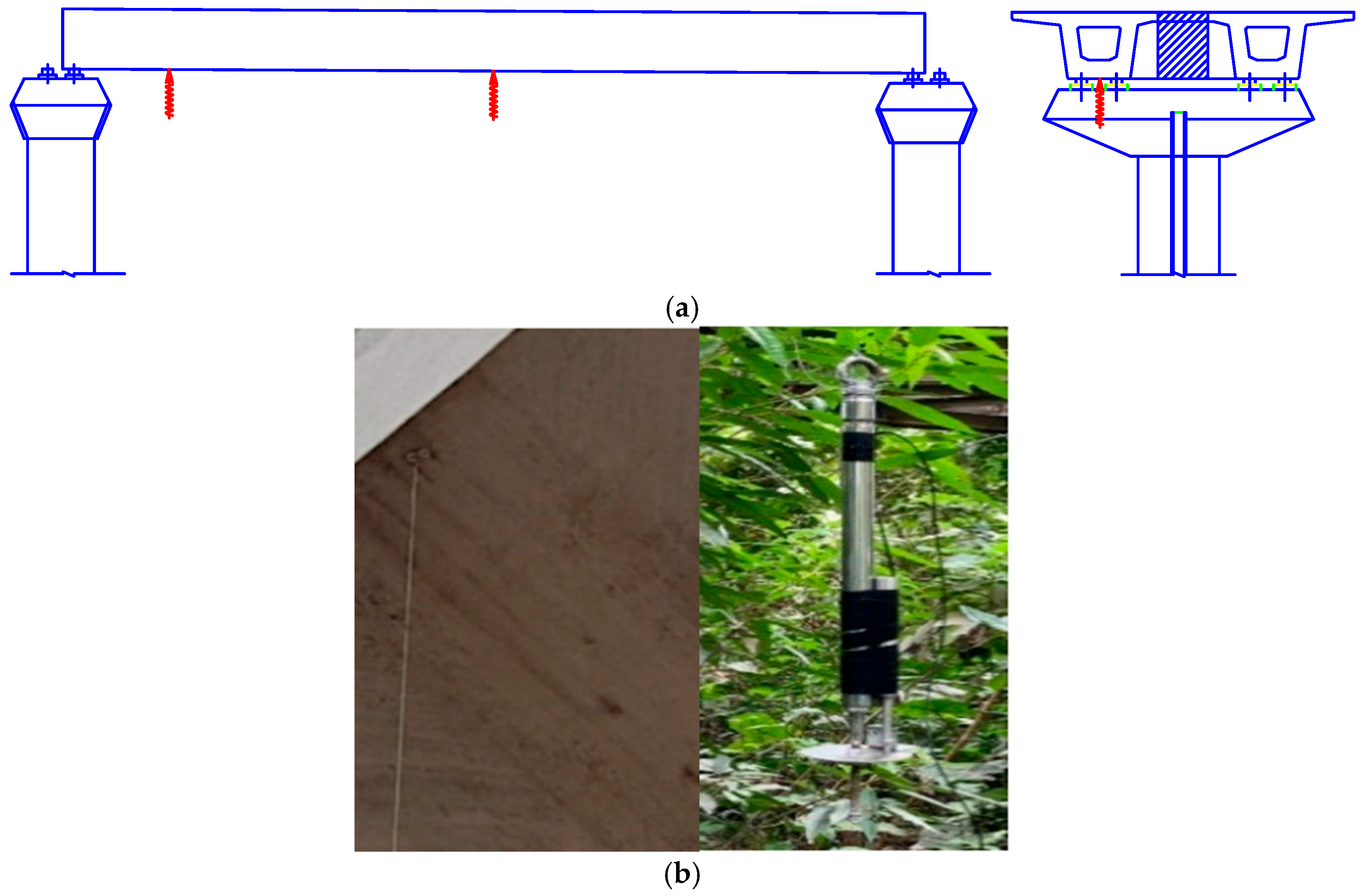
Dynamic displacement data were collected at two locations along the span (Figure 4a). The first location was 5 m from the bridge support. The second location was at the mid-span location. These sensors were strategically placed at the mid-span and near the support positions identified through modal sensitivity and static deformation analyses as being most representative of the bridge’s global and local stiffness characteristics. This configuration provided sufficient information for model calibration while maintaining practicality under field monitoring constraints.

After the equipment is installed, data is continuously recorded, and the segments where trains pass through are extracted for analysis and processing. Figure 4b shows the field data collection.

Data is ensured through temporary pre-processing in the field. In the event of incorrect data, appropriate corrections will be made. In this campaign, data collection was performed twice, and the results were compared. The results showed that the data collection ensured consistency and reliability.

3.2. Update Model to Enrich Data

• Model updating

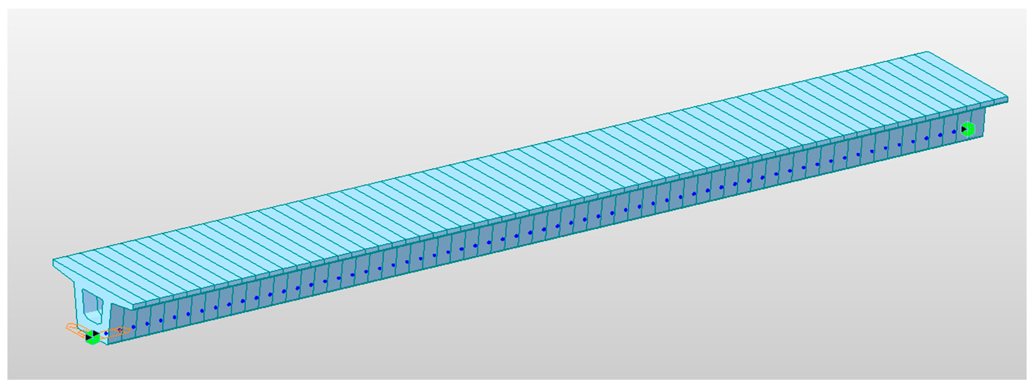
Based on the design documents of the Cat Linh–Ha Dong line and actual field surveys, a first finite element model (FEM) was created (Figure 5) [44,45]. The model uses full parameters and geometric dimensions of the span structure. Material properties are entered with values similar to the design documents. Boundary conditions are declared as bearings with stiffness according to the supplier’s rubber bearings [46].

To improve the reliability of the FEM, a model update procedure was performed. Field-measured displacement data collected from LVDT sensors were used to update the model. The purpose of this procedure was to minimise the discrepancy between the simulated and measured structural responses under actual train loading, thereby ensuring that the numerical model accurately represents the actual dynamic behaviour of the bridge.

Uncertain model parameters, including material modulus of elasticity, moment of inertia, bearing stiffness, and concrete specific weight, are adjusted to update the model. The primary goal of the update process is to minimise the error between the actual and model displacements. The objective function is defined as:

$$J(\theta )=\sum _{i=1}^m\sum _{t=1}^T{w}_i(y_{model,i}(t;\theta )-y_{meas,i}(t){)}^2$$

(14)

Or equivalently, in matrix form:

$$J(\theta )={‖W\circ (y_{model,i}(\theta )-y_{meas})‖}_F^2$$

(15)

where $w_i$: is a weight factor that can prioritise certain sensor locations; $\circ$ denotes the element-wise (Hadamard) product; and ${‖.‖}_F$ is the Frobenius norm. Each w_i was set inversely proportional to the signal variance of sensor i and then normalised so that $\sum w_i=1$. This normalisation ensures consistent scaling across sensors and time, preventing any single sensor from dominating the loss.

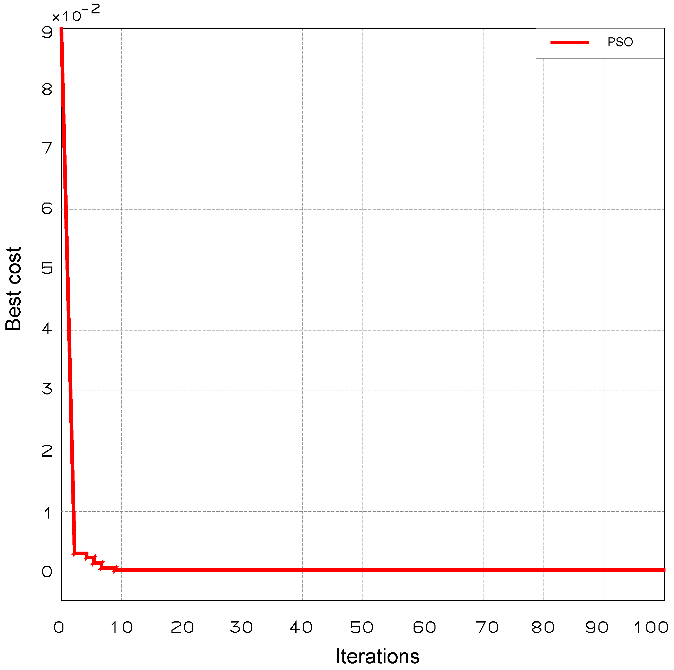
The update procedure is implemented using an iterative optimisation scheme. The updated model is calibrated by comparing the predicted displacements at the sensor locations with actual LVDT measurements under train loading. To address the optimisation problem, this study employs the Particle Swarm Optimisation (PSO) algorithm. The results after updating the model are shown in

Table 1. Uncertain parameter results.

No	Uncertain Parameters	Lower Boundary	Upper Boundary	Initial Value	Updated Value
1	Weight density—ρ (kg/m3)	2400	2500	2450	2469.79
2	Modulus of elasticity—Ec (MPa)	40,000	45,000	40,000	44,539.39
3	Moment of inertia of girder section (I) (mm4)	2.5 × 1012	3.5 × 1012	3 × 1012	2.9626 × 1012
4	Bearing stiffness at support (ks) (N/m)	5.0 × 107	8.0 × 107	7.0 × 107	6.968 × 107

and Figure 6.

b.

Enrich data

After the FEM is successfully updated, the model accurately reflects the actual structural behaviour under train loading. It can be used as a reliable digital twin to generate additional structural response data under different simulated damage scenarios. In this study, data enrichment was performed by systematically introducing different damage types into the updated FEM and generating corresponding synthetic LVDT displacement responses. The damage scenarios were determined by reducing the stiffness of the structural members. The damage levels were simulated at various levels (ranging from 0 to 50% with a 1% interval). Damage locations were also generated across the span structure. For each damage scenario, the model was subjected to the same loading conditions as observed in the field, and the dynamic displacement responses at the LVDT sensor locations were calculated. The resulting dataset includes time series data and structural damage status. Accordingly, single and multiple damage scenarios are performed to enrich the data.

For single damage, the elements are reduced in stiffness, and data is extracted in turn. The formula determines the amount of data:

$$S=n_e\times n_d$$

(16)

where $S$ is the total extracted data, $n_e$ = the total of elements that were considered, and $n_d$ = the number of damage scenarios occurring for a single element.

To further enhance the diversity and realism of the training dataset, multi-damage cases were also introduced. Specifically, combinations of three simultaneously damaged elements were generated based on the group of single damaged locations. The combination formula determined the total number of these multi-damage cases:

$$S=n_d{\displaystyle \frac{n_e!}{k!(n_e-k)!}}$$

(17)

where $S$ is the total extracted data, $n_e$ = the total of elements that were considered, and $n_d$ = the number of damage scenarios occurring, k is the number of damage locations in a combination (here $k=3$). For each combination, the FEM was re-simulated with concurrent stiffness reductions at the selected elements, and the resulting LVDT-like displacement signals were extracted.

The enriched dataset is further normalised and partitioned into training, validation, and testing sets, which are used in the subsequent stage of developing the hybrid 1DCNN-RNN damage detection framework.

The real field data collected from the two LVDT sensors served two purposes: (i) to calibrate and update the finite element (FE) model, and (ii) to provide reference signals for validating the synthetic responses generated by the updated model. After the model updating process, a large synthetic dataset was produced through simulated single- and multi-damage scenarios, resulting in more than 5 million time-series samples. In this dataset, approximately 2% originated from real LVDT measurements, while the remaining 98% were synthetic signals generated from the updated FEM. This ratio ensured that the real data anchored the model to actual bridge behaviour, while the synthetic data expanded the diversity of damage conditions for effective deep learning training. The combined dataset was then randomly divided into training (70%), validation (15%), and testing (15%) subsets. The testing set was kept completely independent from the training process to evaluate the model’s generalisation performance objectively.

3.3. Damage Detection in a Single Damage Case

To ensure methodological transparency and reproducibility, the main hyperparameters and training configurations of the proposed hybrid 1D-CNN–RNN model are summarised in

Table 2. Configurations of the proposed model.

Parameter	Single-Damage (1D-CNN → RNN)	Multi-Damage (1D-CNN → RNN, Deeper)
Optimizer	Adam	Adam
Initial learning rate	0.001	0.001
Loss function	MSE	MSE
Batch size	64	64
Maximum epochs	1000	1000
Early stopping	Not specified (~30 epochs convergence)	Enabled (patience = 10, ~289 epochs)
Data split	Train/Val/Test = 70/15/15%	Train/Val/Test = 70/15/15%
Input	LVDT displacement time series (2 sensors)	LVDT displacement time series
Number of CNN layers	3 convolutional layers	5 convolutional layers
Filters per layer	64 → 128 → 256	64 → 128 → 128 → 256 → 256
Kernel size/Stride	3/default	3/default
Pooling	MaxPooling1D, size = 2 after each conv	MaxPooling1D, size = 2 after each conv
Batch Normalisation	After each conv	After each conv
Activation (CNN)	ReLU	ReLU
Dropout (CNN)	0.2	0.2
Skip/Residual	-	With skip layers (scale = 0.2)
RNN block	2 layers, 128 units each, tanh activation	3 layers, 128 units each, tanh activation

. The parameters were selected through preliminary tuning based on the validation loss and training stability.

In the first evaluation scenario, the hybrid 1DCNN-RNN model was trained and tested on synthetic LVDT displacement data generated from single damage cases. The proposed hybrid model consists of a 1D CNN and an RNN to process the LVDT displacement signal. The 1DCNN module consists of three convolutional layers with 64, 128, and 256 filters, respectively. Each layer uses a kernel size of 3. A ReLU activation function follows it. To down-sample the signal and remove noise, a MaxPooling1D layer with a pool size of 2 follows each convolutional layer. Batch normalisation is applied after each convolution, and a dropout rate (ratio = 0.2) is used to minimise overfitting. The output from the CNN layers is flattened and passed to a two-layer pure RNN. Each RNN layer consists of 128 hidden units using a hyperbolic tan (tanh) activation function. The first RNN layer returns sequences, allowing for the full propagation of temporal features to the second layer, which only outputs the final hidden state. This state is then passed to a dense output layer with linear activation, which produces continuous-valued predictions.

The goal of the model in this task is to predict two continuous variables directly from the displacement signal: (1) the severity of the damage (as a percentage of stiffness reduction), and (2) the location of the damaged element (represented as a normalised spatial coordinate along the bridge span). Model training is performed using the Adam optimiser with an initial learning rate of 0.001. The loss function used is the mean square error (MSE). The model is trained for 1000 epochs with a batch size of 64. The model was optimised using the mean squared error (MSE) loss function, with 70% of the dataset allocated for training, 15% for validation, and the remaining 15% for testing.

Figure 7 illustrates the variation in the loss function during the training process of the single-fault detection model. The graph consists of three lines, corresponding to the training, validation, and testing sets. All loss curves decrease sharply within the first 30 epochs. The model learns the data feature quite quickly due to the 1DCNN-RNN architecture and the clear feature of the LVDT data for single damage. After the 30th epoch, all three lines approach a small value and remain almost unchanged, indicating that the model has achieved stable convergence and is no longer acquiring additional information. The three loss curves (train, validation, test) are very close. The model learns well and generalises well to the data. The final loss value is close to 0. The difference between the prediction and the training dataset is extremely small. The 1DCNN-RNN deep learning model for single damage detection has fast convergence, high accuracy, and no overfitting. It confirms that the spatiotemporal features extracted from LVDT data are robust enough to distinguish single damage states on bridge structures.

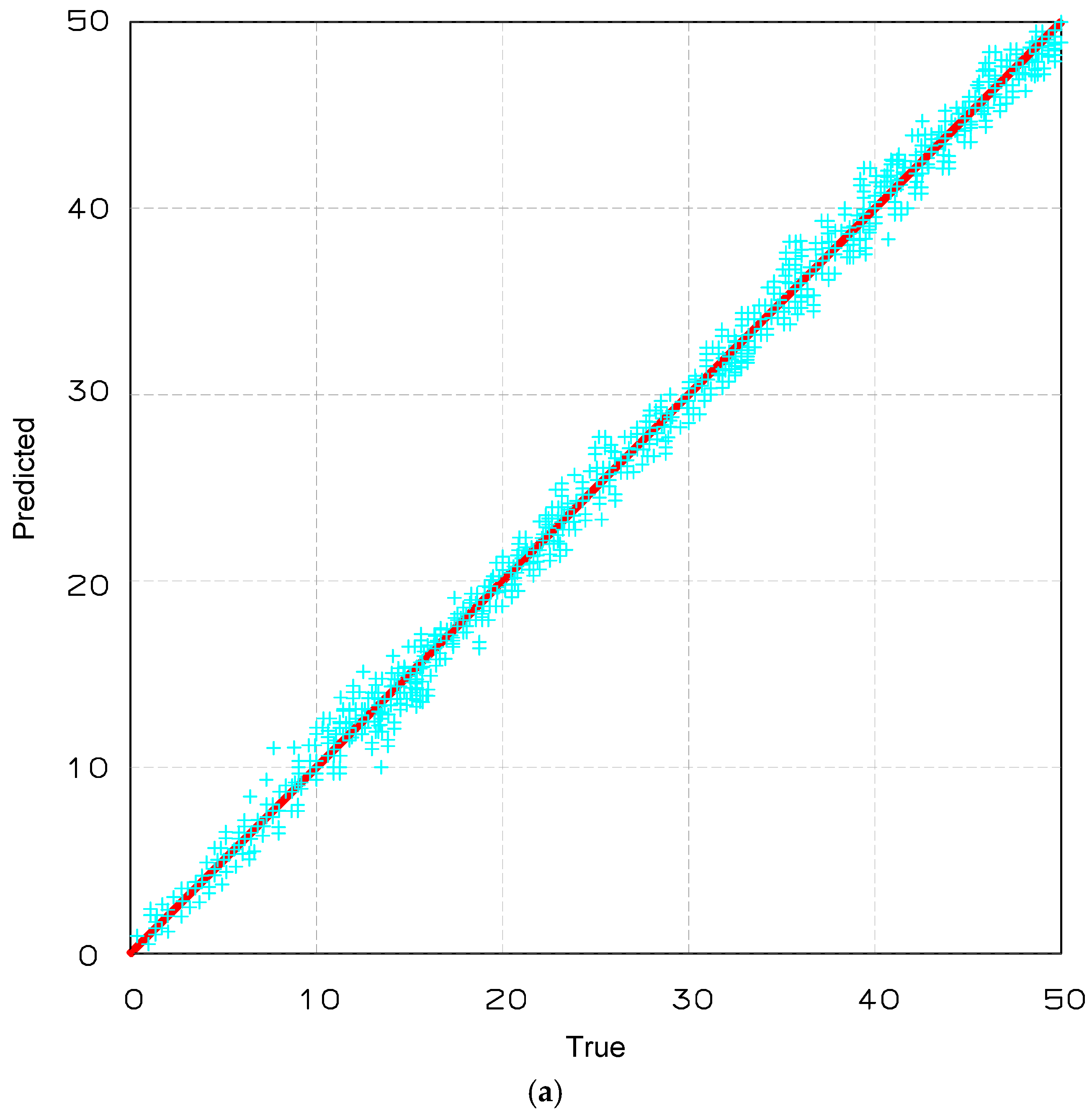
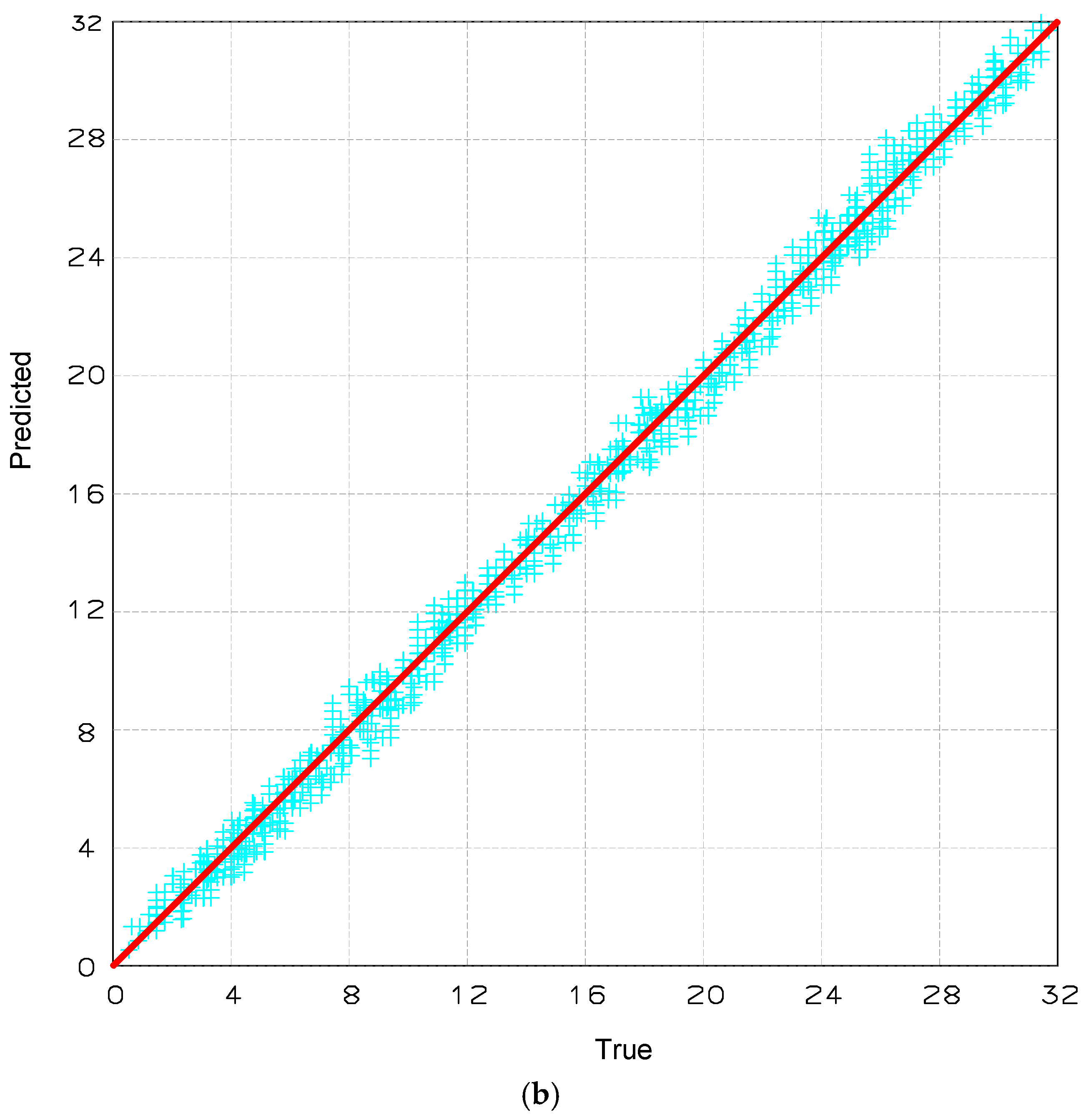
Figure 8 presents the regression performance of the hybrid 1DCNN-RNN model in the single damage detection case. Subfigure (a) illustrates the predicted versus actual damage severity values (expressed as percentage of stiffness reduction), while subfigure (b) shows the regression results for damage location (in metres).

In both subfigures, the red diagonal line represents the ideal reference line where predicted values match the ground truth. The cyan scatter points correspond to the model’s predicted outputs. The plots reveal that the predicted values are closely aligned with the ideal line, indicating high accuracy in the model’s ability to estimate both severity and location of damage.

In particular, the spread of points around the diagonal is minimal, with only slight deviations observed at extreme values. It implies that the model generalises well across the full range of damage intensities and positions. The tight clustering of points further confirms the robustness and precision of the proposed hybrid architecture in capturing damage-sensitive patterns from LVDT displacement signals.

For the single-damage detection task, the hybrid 1D CNN–RNN model achieved an R² value of 0.986, indicating an excellent correlation between predicted and actual damage severity. The MAE and RMSE were 2.8% and 3.4%, respectively, confirming the model’s high accuracy in estimating stiffness reduction levels. The average localisation error across all single-damage scenarios was 0.22 m, demonstrating precise spatial identification of damage along the 32 m span.

3.4. Damage Detection Multi-Damage Case

In the second evaluation scenario, the hybrid 1DCNN-RNN model was extended to handle multiple damage cases involving three simultaneously damaged elements in the structure. To effectively capture more complex spatio-temporal patterns involving multiple damage events, the hybrid model was configured with increased depth and learning capability. The 1DCNN module consists of five convolutional layers with an increasing number of filters: 64, 128, 128, 256, and 256, respectively. Each layer uses a kernel size of 3 and applies the ReLU activation function. A MaxPooling1D layer with a pool size of 2 follows each convolutional layer. Batch normalisation is applied after each convolution, and skip layers (scale = 0.2) are interleaved to improve generalisation.

The final CNN layer’s output is flattened and fed to a three-layer vanilla RNN, each consisting of 128 hidden units with a tanh activation function. The first two RNN layers return the full sequence, allowing for hierarchical temporal learning, while the last layer outputs the final hidden state that summarises the entire time series context. This output vector is fed to a dense fully connected layer with linear activation, producing six continuous values: three representing the damage level and three representing the corresponding damage location.

The model was trained using the Adam optimiser with an initial learning rate of 0.001, while the mean squared error (MSE) was adopted as the loss function. Training was conducted over 1000 epochs with a batch size of 64, and an early stopping criterion with a patience of 10 epochs was applied to mitigate overfitting. The entire dataset, comprising more than 5 million samples, was divided into training, validation, and testing sets, with proportions of 70%, 15%, and 15%, respectively. The results demonstrate that the deeper hybrid architecture successfully models the overlapping and interacting displacement patterns caused by multiple damage locations. The mean absolute error (MAE) for severity prediction is about 3.2%, and the average positioning error is less than 0.7 m. These findings confirm the enhanced modelling capability of the deeper 1DCNN-RNN configuration in detecting multiple damages using LVDT displacement signals.

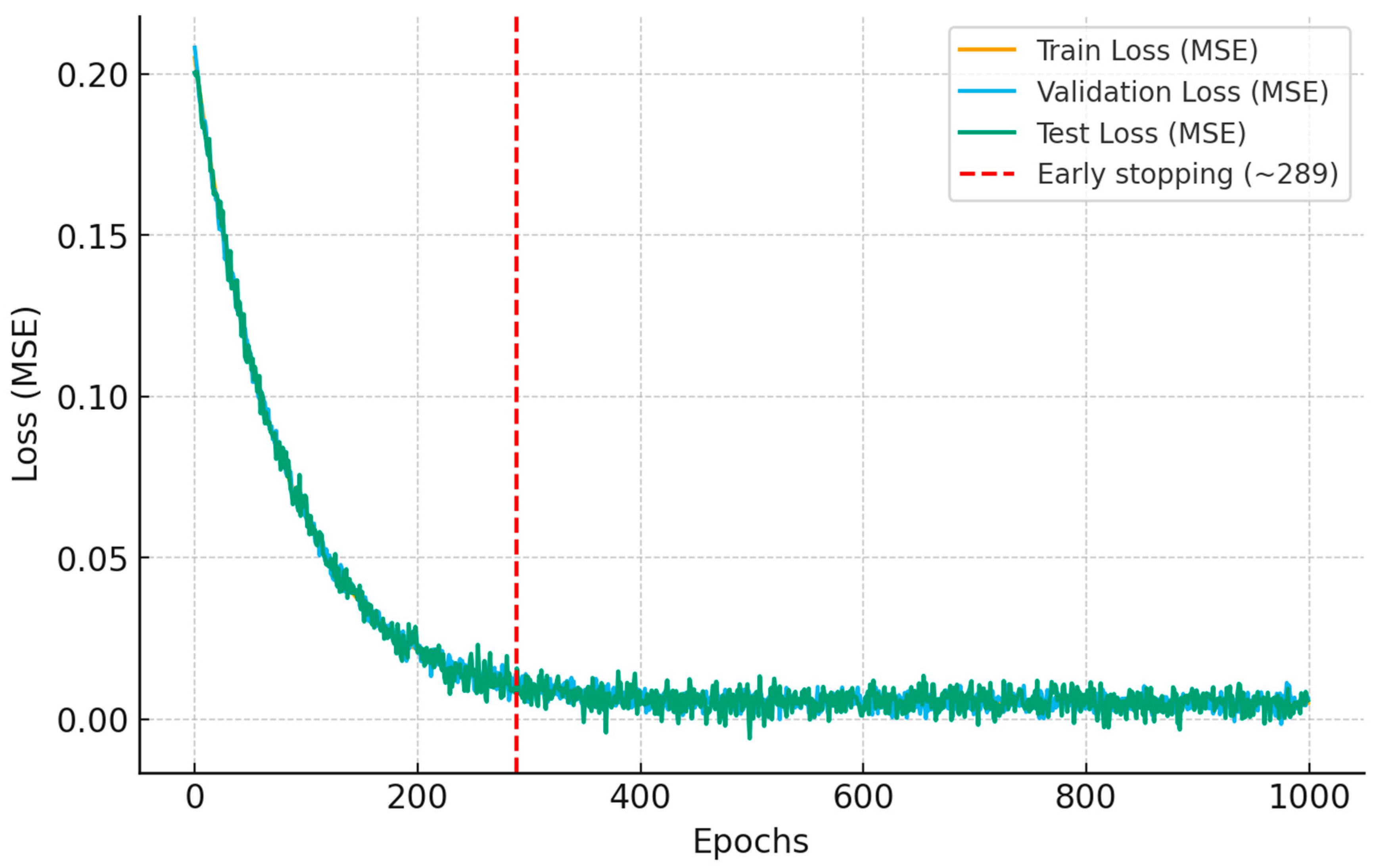
Figure 9 shows the variation in the loss function during training on the synthetic dataset from three simultaneous damage scenarios. Compared to the training graph for single damage, the loss reduction process in this case takes more epochs (289 epochs) to reach a steady state. It reflects the higher complexity of multi-damage data, where multiple stiffness loss locations influence the displacement response, causing characteristic overlap. After convergence, the loss remained stable at a low level for all three sets. It demonstrates that the model has learned the signal variation pattern corresponding to overlapping lesion types, while avoiding overfitting due to the diversity of the enrichment data. The 1DCNN-RNN model still retains its ability to learn spatial–temporal features effectively. It demonstrates that the model structure is flexible and sufficiently deep to extract information in environments with complex and overlapping signals. Although the convergence rate is slower than for single damage, the model still shows good performance in detecting and discriminating complex damage scenarios. It confirms the model’s applicability in real-world conditions, where multiple damages can appear simultaneously.

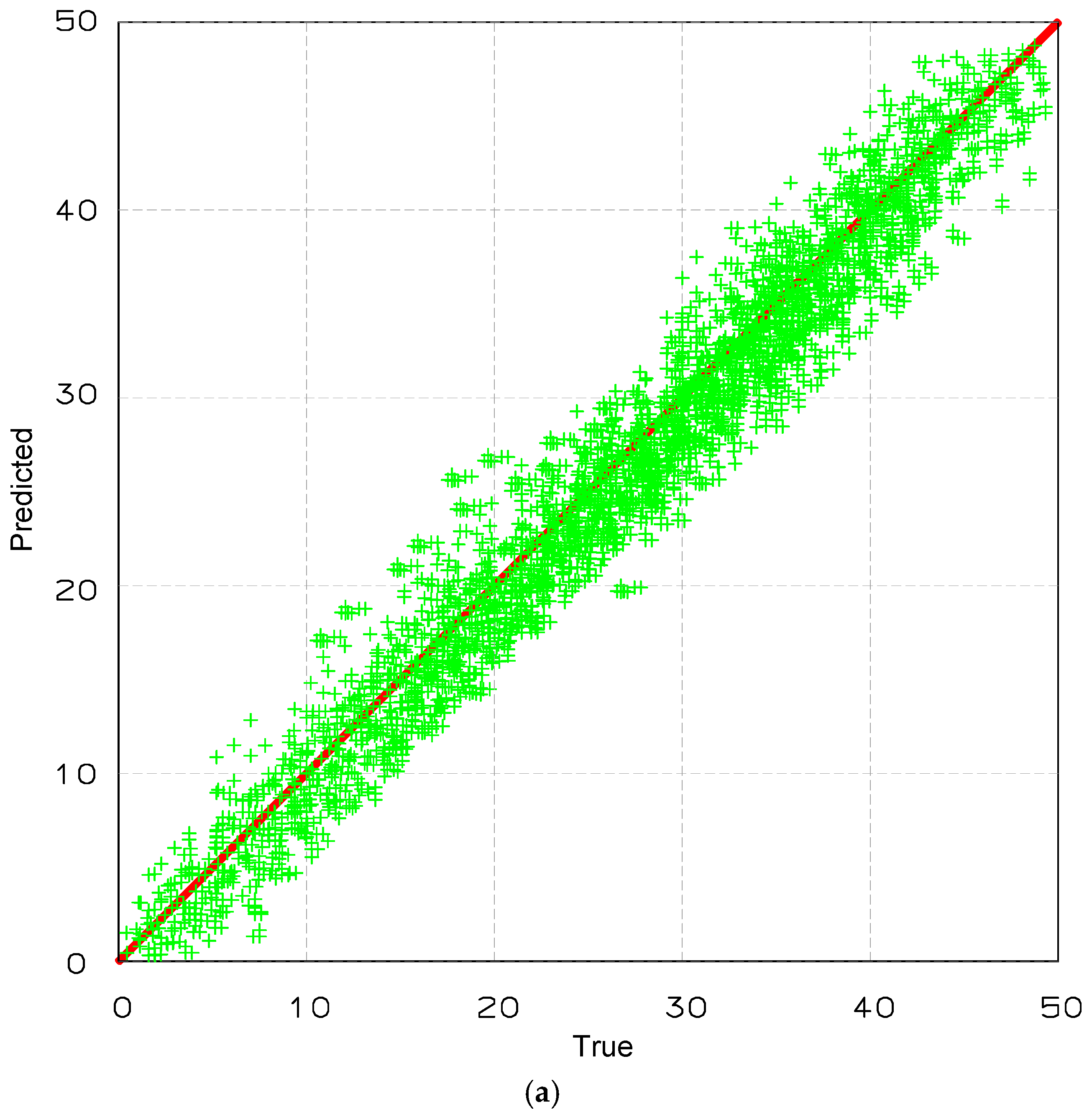
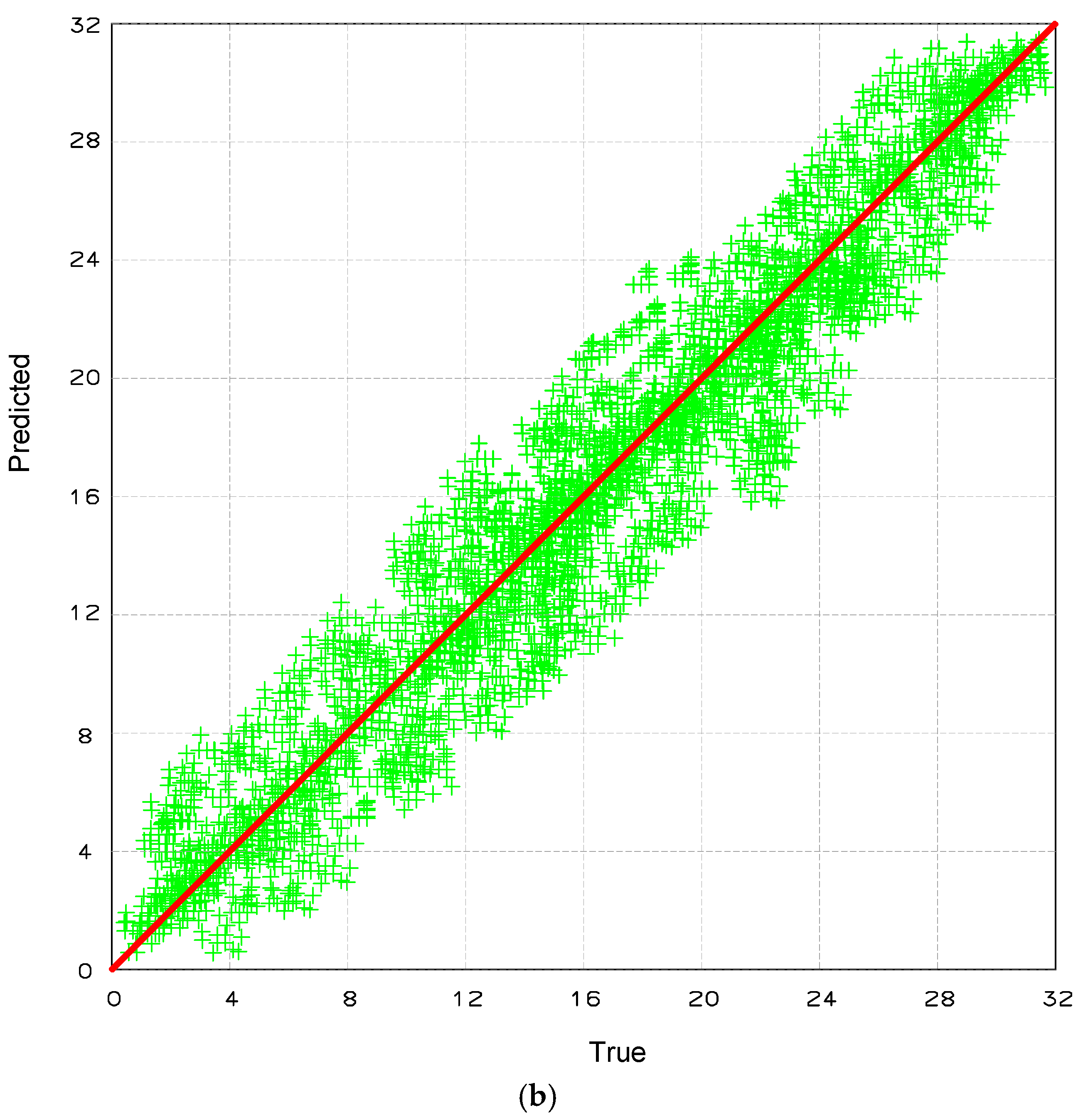
Figure 10 illustrates the regression performance of the proposed 1DCNN-RNN model in the case of multi-damage detection, where three damaged elements occur simultaneously. Subfigure (a) compares the predicted versus actual severity of damage (in % stiffness reduction), while subfigure (b) presents the regression results for the location of the damaged elements (in metres). As shown in Figure 10a, the predicted damage severity values follow the ideal diagonal line closely, though a slightly higher dispersion is observed compared to the single damage case (Figure 9). It is expected due to the more complex interaction between multiple damaged components in the system response. In Figure 10b, the predicted damage locations also exhibit a strong linear relationship with the actual values, but with increased variance and occasional under- or over-prediction, particularly in the mid-span region. Nevertheless, the majority of points remain within a narrow band around the ideal line, confirming that the model can reasonably localise multiple damage positions despite the increased complexity. Overall, the regression plots validate the model’s generalisation ability in multi-damage scenarios and confirm its effectiveness in jointly estimating the severity and location of multiple simultaneous damage events from LVDT displacement signals.

To further assess the effectiveness of the proposed hybrid deep learning framework, additional analyses were conducted by comparing the hybrid 1D CNN–RNN architecture with standalone CNN-only and RNN-only networks trained on the same dataset. The CNN-only model demonstrated fast convergence and strong feature extraction capabilities but exhibited limitations in capturing long-term temporal dependencies, leading to higher prediction variance under complex loading conditions. Conversely, the RNN-only model effectively represented sequential dynamics but required longer training time and was more sensitive to noise and initialisation. In contrast, the hybrid 1D CNN–RNN model achieved the lowest overall prediction error, combining the spatial sensitivity of the CNN with the temporal learning capability of the RNN. Quantitatively, the hybrid model reduced the mean absolute error by approximately 15–20% compared with the individual networks. These results confirm that the proposed hybrid architecture provides superior performance and stability for displacement-based structural damage detection in bridge systems.

Although only two LVDT sensors were employed in this study, their locations were strategically selected based on modal and static sensitivity analyses to capture the most representative displacement responses along the 32 m bridge span. These sensors record the dominant global and local deformation patterns that are highly sensitive to stiffness reductions at various locations. The hybrid 1D-CNN–RNN model then exploits the temporal–spatial correlations in these displacement sequences to infer both the severity and location of structural damage, rather than relying solely on direct spatial coverage. As a result, the model demonstrates strong generalisation even with limited sensing data. Nevertheless, it is acknowledged that a denser sensor network could further enhance spatial resolution and reduce localisation uncertainty in complex multi-damage scenarios. Future research will consider extending the sensor configuration to validate the model’s scalability and robustness under more diverse bridge geometries.

Time–frequency approaches, such as the S-Transform, STIRF, and Band-Variable Filtering, have demonstrated outstanding capabilities in tracking instantaneous modal parameters and identifying transient nonlinear phenomena. The present framework adopts a complementary perspective: instead of explicitly extracting modal features in the time–frequency domain, it utilises a hybrid 1D–CNN–RNN to infer damage-related patterns directly from the raw displacement histories. This implicit learning of time–frequency relationships enables efficient processing of large-scale datasets while maintaining sensitivity to stiffness changes under operational loads. Future developments will explore hybrid models that combine data-driven inference with explicit time–frequency representations to enhance the tracking of strongly nonlinear, non-stationary responses.

Recent advances in nonlinear and non-stationary Structural Health Monitoring (SHM) have introduced powerful time–frequency and adaptive analysis frameworks, such as the S-Transform, Short-Time Impulse Response Function (STIRF), Band-Variable Filtering (BVF), and Hilbert–Huang Transform (HHT), which can estimate instantaneous modal parameters and track their evolution during strong motion or progressive damage [47]. These methods effectively capture transient nonlinear phenomena and distinguish operational variability from true stiffness degradation. In contrast, the present study adopts a linear-based hybrid deep learning model that operates directly on displacement time histories [48,49]. This choice offers simplicity, high computational efficiency, and seamless integration with displacement-based measurements, while allowing the neural network to learn nonlinear effects implicitly from data. Nevertheless, it provides only an averaged representation of strong nonlinearities and is best suited to small-to-moderate vibration amplitudes and minor-to-moderate damage states, where a linearised stiffness–displacement relationship remains physically meaningful. Future work will extend the framework by incorporating explicit time–frequency features to represent transient nonlinear behaviour better.

4. Conclusions

This study proposes a novel framework for structural damage detection in urban railway bridges by integrating LVDT measurements with a hybrid 1D CNN-RNN architecture. The methodology involved updating a finite element model (FEM) using field-measured displacement data to generate a reliable digital twin. This updated model enabled the creation of an enriched dataset covering both single and multiple damage scenarios. The hybrid model was trained and validated on these datasets to predict both the severity and location of damage based solely on dynamic displacement signals. The main conclusions can be summarised as follows:

-

A finite element (FE) model of the Cat Linh–Ha Dong urban railway bridge span was constructed and calibrated using field-measured LVDT displacement data.

-

Synthetic displacement datasets were generated under single and multiple damage scenarios, creating a comprehensive training base for deep learning analysis.

-

Even with only two strategically placed LVDTs, the hybrid model was able to infer both damage severity and location, highlighting its potential for cost-effective SHM systems.

-

For single-damage cases, the severity and location were almost perfectly identified. For multiple-damage conditions, the mean absolute error for severity prediction was about 3.2%, and the average positioning error was less than 0.7 m. These quantitative results confirm that the proposed approach can reliably capture the structural response and provide precise damage identification for urban railway bridges.

Compared to existing studies based on data-based modelling alone, this work demonstrates that incorporating physical features significantly improves the interpretability and reliability of predictions. However, there are still some limitations. The current model was trained using hybrid simulation-measurement data in limited bridge scenarios, and the sensor layout was limited to a few measurement points. Generalisation to other bridge types, loading conditions, and sensor configurations needs to be further validated in future studies. In addition, track–structure interactions and environmental impacts have been simplified in the current formulation. Addressing these factors will be an important direction for future research.