Abstract
Accurate prediction of blast-induced air overpressure (AOp) is vital for environmental management and safety in mining and construction. Traditional empirical models are simple but fail to capture complex meteorological effects, while accurate black-box machine learning models lack interpretability, creating a significant dilemma for practical engineering. This study resolves this by applying explainable AI (XAI) to develop a transparent, “white-box” model that explicitly quantifies how meteorological parameters, wind speed, direction, and air temperature influence AOp. Using a dataset from an urban excavation site, the methodology involved comparing a standard USBM empirical model and a Multivariate Non-linear Regression (MNLR) model against a Symbolic Regression (SR) model implemented with the PySR tool. The SR model demonstrated superior performance on an independent test set, achieving an R2 of 0.771, outperforming both the USBM (R2 = 0.665) and MNLR (R2 = 0.698) models, with accuracy rivaling a previous “black-box” neural network. The key innovation is SR’s ability to autonomously generate an explicit, interpretable equation, revealing complex, non-linear relationships between AOp and meteorological factors. This provides a significant engineering contribution: a trustworthy, transparent tool that enables engineers to perform reliable, meteorologically informed risk assessments for safer blasting operations in sensitive environments like urban areas.
1. Introduction
Blasting is the most common and economical method for excavating rock masses in the mining and construction sectors. However, this technique is highly inefficient in terms of energy conversion. In particular, only 20–30% of explosive energy is used for rock fragmentation and transportation, while most of the rest is released into the environment, creating undesirable effects such as ground vibration, air overpressure (AOp), flyrock, and gas and dust emissions. Among these effects, AOp is one of the most critical environmental problems owing to the structural vibrations and people discomfort caused by low-frequency AOp waves. Therefore, accurate AOp prediction is crucial for conducting blasting operations safely and in an environmentally responsible manner.
The evolution of AOp prediction methods began with empirical equations based on simple functions derived from field observations [1,2,3,4,5,6]. While practically useful, these equations typically include only limited variables such as scaled distance and amount of charge per delay, failing to model non-linear relationships, especially those involving meteorological factors. Numerical modeling methods subsequently addressed these shortcomings and provided higher AOp prediction accuracy [7,8], but their high computational cost, long simulation times, and requirement for specialized setup limit their practical utility.
Over the past two decades, machine learning methods have bridged the gap between the simplicity of empirical models and the accuracy of numerical models. High prediction accuracy has been achieved using artificial neural networks (ANNs), support vector machines, genetic algorithms, adaptive neuro-fuzzy inference systems, and fuzzy logic systems [9,10,11,12,13,14,15,16], with further improvements through hybrid models combining these approaches with learning algorithms [17,18,19,20,21,22,23,24]. However, these models remain opaque and do not allow for direct interpretation of input–output relationships, creating a reliability problem contrary to the principle of interpretability critical for engineering applications.
The atmospheric propagation of AOp is influenced by the physical properties of the medium through which the sound wave passes. Meteorological conditions, while not altering the total energy of the blast, significantly affect AOp levels by governing the distribution and focusing of this energy [2,4]. AOp propagation is primarily dependent on air temperature, wind speed and direction, humidity, and the absorption properties of the air [25,26,27]. Sound waves are refracted in air layers of different densities where the speed of sound changes. An increase in temperature increases the speed of sound. Under normal atmospheric conditions (a negative temperature gradient), sound rays are refracted upward, whereas during a temperature inversion (a positive gradient), they are directed downward [27]. This phenomenon can lead to the focusing of sound waves at long distances (≥1 km), potentially causing 10–20 dB increases in AOp levels [28]. Wind speed and direction are similarly effective, causing sound to propagate faster downwind and slower upwind [27].
Research on meteorological effects on AOp propagation has yielded important insights. Ozer et al. [16] demonstrated a strong correlation (R2 = 0.79) between air temperature and AOp propagation using ANNs, noting that wind speeds below 6 m/s had negligible effect and emphasizing that only dynamic models could represent AOp propagation given meteorological conditions and structural diversity in urban areas. Nguyen et al. [14] identified air humidity as a significant parameter affecting AOp, while Tran et al. [29] found through field measurements that increased air humidity and wind speed, along with falling air temperature, increased blast-induced air overpressure.
The pivotal study by Ozer et al. [16] is of particular importance as it was among the first to successfully model air overpressure propagation by explicitly incorporating meteorological conditions using a black-box ANN. Conducted in the late 2010s, a period marked by the proliferation of black-box machine learning for solving complex engineering problems intractable with classical approaches, their work demonstrated a strong correlation (R2 = 0.79) and confirmed the significant influence of meteorological factors. However, the model’s opaque nature meant that while the existence of a relationship was confirmed, its specific quantifiable form remained hidden within the network. This created a critical gap between scientific insight and practical engineering application. Although meteorological conditions were used for prediction, their quantitative effects remained undetermined, and no usable, transparent equation was provided to the reader. Consequently, the functional relationships between inputs and outputs, and even the interactions among the inputs themselves, were largely unknown. This fundamental limitation of the black-box approach, applied to a foundational dataset that first confirmed the role of meteorology, created a compelling necessity and opportunity for a secondary evaluation of the same data using modern explainable AI (XAI) techniques.
This gap precisely created the secondary evaluation necessity and opportunity for the dataset of Ozer et al. [16]. The recent proliferation of white-box XAI methods, particularly Symbolic Regression (SR), now enables bridging this critical gap. While the black-box ANN of the late 2010s provided a powerful predictive solution, it failed to reveal how that solution was achieved. In stark contrast, SR autonomously extracts and expresses complex non-linear interactions as explicit, interpretable, and physically meaningful mathematical formulas directly usable by engineers. This white-box approach not only quantifies the numerical effects of input parameters but also delivers a final, actionable formula for end-users. Furthermore, and crucially, it autonomously discovers and quantifies complex, non-intuitive relationships and mathematical formulations that might elude human reasoning or be deemed ‘unthinkable’ by human researchers. The ability of SR to generate such novel formulations, as evidenced by the distinct and complex terms (Term 1, 2, and 3) in the final SR equation of this study, thereby establishes new grounds for scientific debate and discovery, particularly among researchers focused on blast-induced air overpressure, moving the field from mere prediction towards genuine data-driven discovery.
The emerging field of XAI addresses the “accuracy-interpretability” dilemma in machine learning by making AI algorithm decisions understandable and transparent to humans [30]. SR represents a key XAI technique that simultaneously discovers the structure and parameters of mathematical expressions explaining data without predefined model constraints [31]. SR produces explicit, analytical “white-box” formulas rather than black-box models, enabling experts to debate, refine, and validate components against domain knowledge. Crucially, SR can uncover non-intuitive, complex relationships between variables that may elude human researchers. Typically implemented using evolutionary algorithms like genetic programming [32] or gene expression programming [33], SR evolves candidate equation populations over generations through crossover and mutation, progressively improving predictive accuracy [31,32].
White-box methods have demonstrated significant potential across blasting and geotechnical engineering applications. In geotechnical engineering, successful SR applications include slope stability analysis [34], rock mechanical properties prediction [35], tunneling total loads modeling [36], mining/tunneling-induced surface subsidence prediction [37,38], and anisotropic closure analysis in deep tunnels [39]. In blasting engineering, Faradonbeh et al. [40] showed GEP-derived symbolic regression equations provided higher accuracy than multivariate non-linear regression for ground vibration prediction. Monjezi et al. [41] proved their GEP-derived ground vibration propagation equation outperformed linear and non-linear regression equations, while Shakeri et al. [42] demonstrated GEP-based ground vibration models surpassing black-box ANNs. For AOp prediction specifically, Faradonbeh et al. [13] showed GP and GEP equations succeeded over traditional methods, and Kazemi et al. [43] found GEP achieved the highest test dataset results compared to empirical and black-box models.
While existing SR studies in blasting demonstrate its predictive power, they often focus on relationships with a strong prior conceptual grounding in traditional blasting mechanics, such as scaled distance for vibration prediction. The present study addresses a more challenging and exploratory problem: autonomously discovering and explicitly quantifying the complex, non-linear coupling between AOp and meteorological parameters (wind speed, direction, temperature). This represents a step beyond mere prediction into the realm of data-driven discovery of new physical relationships. This need is powerfully underscored by Ozer et al.’s [16] black-box ANN model, which confirmed the influence of meteorological factors but left their specific quantifiable form hidden within the network.
Existing AOp prediction approaches thus reveal a dual limitation: empirical equations are insufficient for modeling complex meteorological effects, while black-box machine learning methods cannot provide the transparent equations required for engineering trust and application. SR overcomes both limitations by capturing intricate non-linear relationships directly from data while producing open-form equations. These equations reveal hidden relationships among complex AOp-affecting parameters, potentially discovering interactions previously unknown or unquantifiable by human experts. This unique capability for autonomous discovery, generating formulations that human intuition might not conceive (as evidenced by the complex terms in the final SR equation), necessitated a secondary, explainable evaluation of the dataset from our previous black-box study [16]. The primary aim was to provide field engineers with not just an accurate, but a transparent and trustworthy model for reliable, meteorologically informed risk assessment in sensitive urban blasting operations.
To validate this approach, the SR model is compared against the classical USBM equation and a multivariate non-linear regression (MNLR) model using the same dataset, examining SR’s predictive success and meteorological parameter incorporation improvements. Model performance is evaluated on an independent test set using R2, RMSE, and MAE metrics, with additional comparison to the black-box model from Ozer et al. [16].
This study represents a significant advance in blast-induced AOp prediction by developing an explainable AI method incorporating complex meteorological parameters into a physically interpretable model. The primary contributions include: (a) developing a white-box SR model overcoming the accuracy-interpretability dilemma in black-box machine learning and traditional empirical equations, explicitly capturing non-linear hidden relationships between AOp and meteorological parameters like air temperature, wind speed, wind direction, and source-receiver angle through a physically interpretable mathematical formula; (b) comparing the proposed SR model’s predictive success against traditional methods (classical USBM equation and MNLR model) and the previously developed black-box ANN model [16] on the same dataset, demonstrating effectiveness using R2, RMSE, and MAE metrics; and (c) presenting a practical engineering tool that is both highly accurate and transparent, enabling blasting engineers to conduct reliable meteorological condition-aware risk assessments, particularly relevant for urban areas and directly applicable in the model’s development field.
2. Materials and Methods
This section will detail the steps of the research methodology applied to derive equations including meteorological parameters for predicting blast-induced AOp. The general workflow followed in the study can be visualized via the flowchart presented in Figure 1. Each section is detailed under sub-headings.
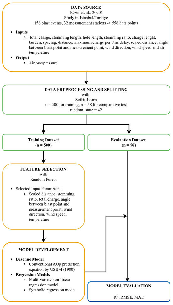
Figure 1.
Overall workflow followed in the study [2,16].
2.1. Study Site and Data Supply
The dataset used in this study was obtained from research conducted by Ozer et al. [16,44]. In this study, data were collected at an active excavation site in Istanbul, Turkey’s largest metropolis, over an eight-month period between October 2014 and August 2015. A total of 158 blasting shots were observed at this site, which geologically belongs to the Thrace Formation and mainly comprises “Grayvake series” rocks with different degrees of weathering belonging to the Devonian period. A total of 558 air pressure events were measured with Instantel Minimate Plus instruments at 32 strategically located measuring stations to record the propagation of air pressure waves caused by the blasts in multiple directions. In addition, daily meteorological condition data (air temperature and wind speed and direction) were obtained from the Turkish State Meteorological Service and included in the employed dataset [16,44].
In this study, the aforementioned dataset was selected because it has a large measurement volume, reflects blasting excavation activities in an urban area, and contains meteorological condition parameters for different time periods. These characteristics of the dataset provide a solid foundation for the objectives of this study. The dataset includes the wind direction (β) parameter in the range of 1–8 based on the directions presented in Figure 2. In this study, the midpoint angles corresponding to these directions were used to determine the numerical effects (e.g., direction 1 = 22.5° and direction 8 = 337.5°). Since machine learning models may interpret these 1–8 values linearly, sine–cosine transformations were applied to the angular variables to accurately represent their cyclical nature. However, the dataset has some limitations. Studies conducted [14,29] have reported that air humidity considerably affects AOp. This parameter is not included in the dataset used in this study.
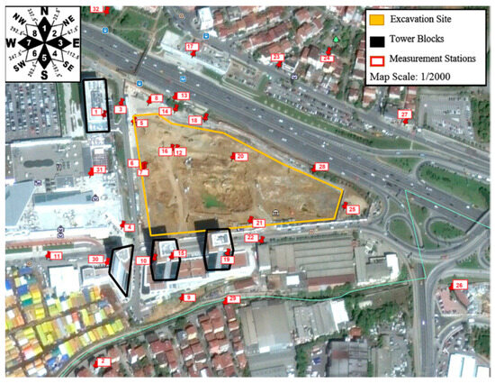
Figure 2.
Excavation site [16]. (The excavation site is outlined in yellow, the “Tower Blocks” are indicated by black polygons, and the numbered red boxes represent the measurement stations. The compass rose in the top-left corner indicates orientation).
The statistical summary of the dataset is provided in Table 1. The image showing the excavation site where the dataset was obtained is presented in Figure 2.

Table 1.
AOp dataset used in this study [16,44].
2.2. Data Preprocessing and Splitting
The raw dataset contained 562 observations in the first stage, and 558 observations were used in the analysis after removing 4 observations with missing metadata. To objectively evaluate the performance of the developed models on unknown data, the main dataset comprising 558 observations (Table 1) was randomly divided into two distinct sets. In this context, 500 observations (Table 2) were utilized as the development set for the derivation of all models. 58 observations (Table 3), corresponding to approximately 10% of the total data, were randomly allocated as the evaluation set. This dataset was set aside and was not used in any stage of model development, feature selection, or hyperparameter optimization. The final generalization performance of the models was measured only on this blind dataset The randomness and scientific reproducibility of this data separation process were implemented using the scikit-learn (Version 1.7.0) library.
Table 2.
Training dataset.
Table 3.
Evaluation dataset.
2.3. Feature Selection with Random Forest (RF)
To improve the performance of the AOp prediction models, reduce computational complexity, and identify the most influential parameters affecting the output variable, a feature selection process was applied on the training dataset (n = 500) from an initial set of 14 input variables. As frequently reported in the literature, feature selection improves model performance and removing unnecessary variables reduces computational cost and improves interpretability [45]. In this study, RF, which is an ensemble learning method based on decision trees, was utilized as a pre-filter to determine attribute importance scores. RF’s ability to reliably measure variable significance and perform efficient feature selection in high-dimensional datasets makes it a suitable method for this purpose [46].
To ensure the reliability of the aforementioned process, the RF model itself was first subjected to hyperparameter optimization. The optimal hyperparameters were determined using the RandomizedSearchCV technique and 10-fold cross-validation. The results confirmed that the optimized RF model showed a high performance on the training data (R2 = 0.928) and achieved significant success on the test data (R2 = 0.701). This suggests that the model is a suitable tool for reliably determining attribute importance scores. This difference in achievement between the training and test metrics was considered an acceptable margin of memorization because the purpose of using RF in this study was only to determine the relative importance ranking (hierarchy) of the input variables in predicting AOp.
Using the best model obtained after optimization, the importance scores showing the contribution of each input variable to the prediction process were calculated. Figure 3 shows the contribution of each attribute to the output variable.
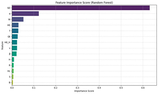
Figure 3.
Random forest feature ranking. (B: Burden (m); S: Spacing (m); Qt: Total charge (kg); H: Hole depth (m); H0: Height of stemming (m); H0/H: Stemming ratio (m/m); Hc: Height of charge (m); W: Charge amount per delay (kg); R: Distance (m); SD: Scaled distance (m/(kg)1/3); α: Angle (°) between the blasting point and the recording point, β: Wind angle (°); v: Wind speed (m/s); T: Air temperature (°C)).
The input parameters of the best model were subjected to a careful selection process, taking into account their RF attribute rankings and physical significance. In this process, the parameters included in and excluded from the model are explained below with their justifications.
Parameters Included in the Model
- Scaled Distance: This parameter is a composite parameter combining the physical distance to the blast point and the amount of charge per delay. Moreover, it represents the effects of two parameters highly efficiently, and its use alone rather than as two parameters was preferred for reducing model complexity.
- Meteorological Impact and Orientation Parameters: The air temperature, wind speed, wind direction parameters, and the direction parameters between the blasting point and the receiver were included in the model considering their (i) importance scores obtained using the RF model and (ii) inclusion of the meteorological effects that form the basis of this study.
- Stemming Ratio: According to the RF results, although the stemming depth is a more meaningful parameter on its own, to avoid increasing model complexity, instead of using the stemming depth and hole depth parameters at the same time, the stemming ratio, which is a more physically meaningful representation of the rate energy confinement rate in the hole, was preferred.
- RF results showed that Qt has a significant effect on AOp. However, this situation contradicts the principle that in a controlled blasting site, Qt should not physically affect AOp. To convert this contradiction into a methodological test, Qt was deliberately not removed from the feature set. Instead, it was decided to include this variable in the subsequent modeling stages (MNLR and SR). The aim here was to see whether traditional statistical models like MNLR would assign a statistical significance to this physically meaningless variable, and to test if the more flexible SR model could autonomously eliminate this variable from the equation despite its high importance score from RF. This approach was designed to confirm SR’s ability to filter out physically irrelevant inputs.
Parameters Excluded from the Model
- Parameters with low importance scores such as burden, space between blast holes, and charge height were removed from the model to simplify the model and increase its efficiency by removing noise.
Table 2 and Table 3 present the summary information of two separate datasets containing 500 and 58 data points, which were obtained as a result of data segmentation and feature selection processes and were reserved for model development and testing. Furthermore, Figure 4 displays the histograms comparing the distribution of each input parameter for these training and evaluation datasets.
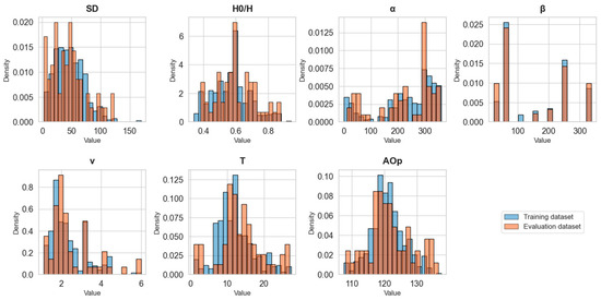
Figure 4.
Distribution comparison between training and evaluation datasets for each input parameter. (SD: Scaled distance (m/(kg)1/3); H0/H: Stemming ratio (m/m); α: Angle (°) between the blasting point and the recording point, β: Wind angle (°); v: Wind speed (m/s); T: Air temperature (°C); AOp: Air overpressure (dB). The blue bars represent the training dataset, the orange bars represent the evaluation dataset, and the darker areas indicate the overlap between the two distributions).
2.4. Development of Prediction Models
After the preprocessing and feature selection steps, three AOp prediction models were developed using the seven selected input parameters. The USBM empirical equation was selected as a reference point representing the standard approach in the industry. MNLR was included to analyze how meteorological parameters play out in a traditional statistical framework. Furthermore, SR served the main objective of this study was, developing a flexible and interpretable model that learns from data without a predefined structure.
2.4.1. Reference Model: USBM Equation
For a fair comparison of the proposed model, the conventional USBM equation, which is widely used in AOp prediction, was selected as the reference model. Site-specific k and ß numbers were determined by performing an exponential regression analysis on the AOp and SD values from the 500-point model development dataset (Table 2). The exponential regression yielded the site-specific parameters k = 286.53 and β = −0.693. The derived USBM equation, AOp = 286.53 × (SD)−0.693, achieved an R2 of 0.599 on the training data.
2.4.2. Proposed Model 1: MNLR Model
The first model (MNLR model), which is one of the main outputs of this study, was developed using the IBM-SPSS (Version 27.0.1.0) software package on the dataset containing 500 data points (Table 2). The MNLR procedure was applied in this process. Consequently, a clear and interpretable mathematical equation was obtained that expresses AOp as a function of seven input variables.
The MNLR model was constructed as a multivariate power function structure. The constructed model is y = k × (x1)a × (x2)b × (x3)c × (x4)d × (x5)e × (x6)f × (x7)g. The multivariate power function structure was preferred owing to its ability to model complex relationships (attributable to the flexibility it provides with respect to multivariate and non-linear systems), physical significance, and coefficient interpretability.
2.4.3. Proposed Model 2: SR Model
In this study, Python (Version 3.11.9) and Python-based symbolic regression tool (PySR) (Version 1.5.9) was used to derive the SR equation. PySR is a Python-based symbolic regression tool that employs evolutionary algorithms to generate interpretable, closed-form equations from data [47]. Compared to classical symbolic regression approaches such as genetic programming or other evolutionary methods, PySR offers advantages in computational efficiency through parallel processing, seamless integration with the Python ecosystem, flexibility in including user-defined functions, and automated model selection, making it particularly suitable for data-intensive engineering applications.
In the PySR model, an input set derived from the seven main variables identified in the feature selection step was used. To enable the model to more accurately interpret the cyclic nature of the angular data (α and β), these variables were decomposed into sine and cosine components using pre-training feature engineering instead of using them directly.
This is a standard feature engineering technique that ensures the model correctly interprets the proximity of boundary values (e.g., 359° and 1°) by preserving the cyclical nature of periodic data, and its benefits are well-documented in engineering applications [48].
Through this transformation, the search space of the model was also narrowed, and the sine and cosine components were added to the singular operators, preventing the model from trying to assign these operators to non-angular parameters. Because the Python programming language works in radians for angles, the angles were converted into radians.
Consequently, the final parameters that constitute the input set of the model were determined as SD, H0/H, Qt, T, v, sin(α), cos(α), sin(β) and cos(β). During the development of the PySR model, the main training set (n = 500) was temporarily subdivided into a 400-sample set for model training and a 100-sample set for internal validation. This internal validation set was used for tasks such as monitoring model convergence and assisting in the selection of the final equation from the “hall of fame”. The final, comparative performance of the fully developed PySR model was then benchmarked on the separate, independent evaluation set (n = 58), ensuring consistency with the other models in this study.
The hyperparameters for the PySR model were selected to balance computational efficiency with a thorough exploration of the equation space. A population size of 500 and 5000 iterations were chosen to allow sufficient generational evolution without prohibitive computational cost. The set of operators (+, −, *, /, ^, square, sqrt, etc.) was chosen to encompass a wide range of potential physical relationships observed in blast dynamics. The constraints, such as limiting the exponent in the power operator (^: (1, 1)), were implemented to promote numerical stability and enhance the physical plausibility of the resulting expressions. The parameters used in the model setup and their values are presented in Table 4.
Table 4.
PySR installation parameters.
The final equation produced was not automatically selected. Instead, PySR generated a “hall of fame” list showing accuracy scores versus complexity. This list of candidate equations was manually examined. From this list, the equation that represented the best balance between prediction accuracy, model complexity, and physical interpretability was deliberately selected.
2.4.4. Model Validation
R2, RMSE, and MAE statistical performance metrics were used to evaluate the prediction accuracy and reliability of the developed models on the evaluation dataset.
where n is the total number of observations, is the recorded air shock value, is the predicted value, and is the average of the measured values.
3. Results
3.1. Developed Models and Derived Equations
To enable a comprehensive comparison, three predictive models were developed: the conventional USBM empirical equation, a MNLR model, and a SR model. The explicit forms of the derived equations are presented below.
3.1.1. USBM Empirical Equation
The site-specific USBM model was obtained by exponential regression of the SD and AOp values from the training dataset. The regression analysis graph is presented in Figure 5. The resulting equation is presented in Equation (4). The R2 score of the equation is 0.599.
AOpUSBM = 286.53 × (SD)−0.693
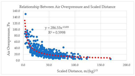
Figure 5.
AOp–SD relationship. (The blue circles are the measured observations of AOp versus scaled distance (Table 2). The red dotted line represents the fitted power-law regression curve).
3.1.2. MNLR Model
The MNLR model was constructed in a multivariate power function form using seven selected variables. The model obtained as a result of the analysis was found to be significant (F (8, 492) = 86.306; p < 0.001). The model explains 60.0% of the variance (R2 = 0.60). The model obtained is presented in Equation (5).
AOpMNLR = 137.888 × (SD)−0.049 × (H0/H)−0.016 × (Qt)0.001 × (α)0.002 × (β)0.005 × (v)0.004 × (T)−0.002
Table 5.
MNLR parameter predictions.
Table 6.
MNLR ANOVA results.
3.1.3. SR Model
As detailed in the Methodology (Section 2.4.3), the PySR algorithm generated a “hall of fame” of candidate equations ranked on a Pareto front. From this list, the final model (Equation (6)) was selected.
The equation with the absolute lowest loss score is typically highly complex and prone to overfitting. Therefore, the equation presented in Equation (6) was not chosen for having the lowest loss but was deliberately selected from the hall of fame as representing the optimal trade-off between model parsimony (low complexity) and predictive accuracy (low loss).
The robustness of this choice is supported by the performance metrics: the model yielded an R2 score of 0.687 on the training dataset and a very close score of 0.680 on the test dataset. This narrow gap between training and test performance indicates that the model generalizes well and is not overfit.
The final proposed equation (Equation (6)) is structured as the sum of three distinct terms: a wind-angle term (Term 1), a scaled distance term (Term 2), and a complex interaction term (Term 3).
where
Physically, the equation can be interpreted as the summation of three primary components: a directional wind effect (Term 1), a logarithmic distance attenuation term (Term 2), and a complex interaction term (Term 3) that encapsulates the interplay between blast geometry, stemming efficiency, wind speed, and temperature. A detailed, step-by-step calculation example demonstrates the practical application of Equation (6) is provided in Appendix A.
3.2. Model Evaluation Results on Evaluation Dataset
The dataset used in this study comprised 558 blasting observations; the comparative evaluation of the models was performed on 58 independent blasting data (Table 3). The performance metrics used in the analyses were R2, RMSE, and MAE; the results are summarized in Table 7.
Table 7.
Statistical performance metrics of equations.
The performances calculated on the independent evaluation test set (n = 58) are summarized as follows: USBM R2 = 0.665 (RMSE = 3.940 dB; MAE = 3.013 dB), MNLR R2 = 0.698 (RMSE = 3.741 dB; MAE = 2.716 dB), and SR R2 = 0.771 (RMSE = 3.259 dB; MAE = 2.496 dB). A comparative visualization of the measured AOp values and model AOp predictions is presented in Figure 6.
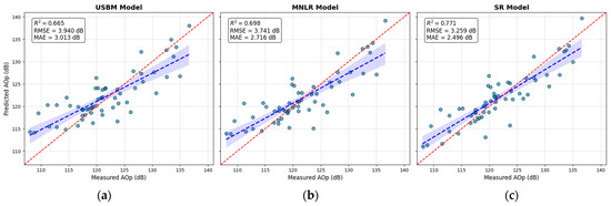
Figure 6.
Comparison of predicted versus measured AOp values for the (a) USBM, (b) MNLR, and (c) SR models. The blue circles represent the individual observations from the evaluation dataset (n = 58). The red dashed line indicates the 1:1 line of perfect agreement, while the shaded area around the regression line (blue dashed line) represents the 95% confidence interval.
3.3. Parametric and Stability Analysis
To further evaluate the sensitivity of the developed equations to changes in input parameters, a parametric analysis was carried out by decreasing and increasing each variable from a reference point. The corresponding effects on the predicted AOp values are presented in Table 8. This table allows a direct comparison of the response of the USBM, MNLR, and SR equations to systematic parameter variations.
Table 8.
Effects of parameter changes on equation prediction results.
The numerical stability of the model was also validated on an independent test set. Boundary tests were performed using the min–max ranges of all variables. The expression sin(β) in the denominator in the case of β → 0° and 180° in the SR model may be theoretically problematic, but it does not lead to numerical instability because the smallest β is 22.5° in the dataset. The results are presented in Table 9.
Table 9.
Model stability test results.
4. Discussion
The Symbolic Regression (SR) model developed in this study achieved a predictive performance of R2 = 0.771 on the independent evaluation dataset. The significance of this contribution must be evaluated by contextualizing this result against two different categories of models present in the literature: other high-performing “white-box” models and “black-box” models used on similar complex datasets. At first glance, this R2 value may appear modest compared to the exceptionally high performance reported in other “white-box” (SR/GEP) studies on blast-induced AOp, such as Faradonbeh et al. [13] (R2 = 0.941) or Kazemi et al. [43] (R2 = 0.989). However, this apparent discrepancy is not a limitation of the SR method but rather a direct reflection of the inherent complexity and “noise” of the dataset being modeled. Both the Kazemi et al. [43] and Faradonbeh et al. [13] studies did not incorporate complex meteorological parameters. Furthermore, our dataset is derived from a dense urban environment. As Ozer et al. [16] confirmed using this exact same dataset, the surrounding high-rise structures create a “barrier effect” and irregular wave propagation, making the data inherently more complex and challenging to model than a standard open-pit mine. Therefore, achieving an R2 of 0.771 in such a challenging, real-world urban and meteorological context represents a significant modeling success.
The most robust and direct evaluation of our model is the comparison with Ozer et al. [16], which used the same complex dataset but employed a “black-box” ANN. Ozer et al. [16] achieved an R2 = 0.79, while our “white-box” SR model achieved R2 = 0.771. This finding is central to our study’s contribution: we have successfully resolved the “accuracy–interpretability dilemma.” Our SR approach delivers predictive accuracy that is highly competitive with a high-performing black-box model. In exchange for this negligible trade-off, our model provides what the ANN cannot: a fully transparent, explicit mathematical equation that is physically interpretable and can be directly audited and applied by engineers. This study’s approach also demonstrated superior discovery power compared to the previous black-box analysis. Notably, Ozer et al. [16], despite using the same data, concluded that wind direction had no significant effect within the observed range. In contrast, our SR model autonomously discovered a strong, non-linear relationship and incorporated it into the final equation. This discrepancy highlights a key advantage of white-box models: their ability not just to predict, but to reveal influential parameters and their functional form. This discovery was enabled by our physically informed preprocessing (sine-cosine transformation of wind direction), which allowed the SR algorithm to correctly interpret the cyclical data and uncover a relationship that was present and physically plausible, yet missed by the black-box ANN. This finding validates the need for a secondary, explainable evaluation of complex datasets.
The SR model’s success becomes even more apparent when contrasted with the fundamental limitations of traditional regression. The Multivariate Non-linear Regression (MNLR) model (R2 = 0.698) was constrained by its pre-defined power-law form, which acted as a straitjacket, preventing it from adequately quantifying the non-linear meteorological effects. This failure is evident in its 95% confidence intervals, where the coefficients for wind speed (v) and air temperature (T) were found to be statistically insignificant. The fact that some MNLR coefficients were insignificant and that the exponents of several variables were extremely small suggests that its rigid structure was unable to capture the complex influences present in the data. It should also be noted that the measured AOp values in this study span a narrow range (107.50–137.50 dB), which naturally reduces the magnitude of the derived coefficients. Nevertheless, from a practical standpoint, even small changes cannot be dismissed. Due to the psycho-acoustic response of humans, an increase of only 1 dB in AOp can be perceived as a much larger increase, a critically important consideration for the urban excavation site examined in this research. Therefore, identifying and modeling any parameter that can influence AOp, even if its coefficient appears small, is essential for reducing community disturbance. This limitation, however, directly supports the motivation for this study: it highlights the shortcomings of traditional models and emphasizes the need for flexible approaches like SR The SR equation yielded an R2 score of 0.687 on the training dataset and 0.680 on the test dataset; this small difference indicates that the model does not overfit and is generalizable to new data.
The structure of the final SR equation may appear complex and non-intuitive at first glance. It is precisely this complexity, however, that underscores its role as a powerful discovery tool, autonomously generating formulations that human intuition might not conceive. Unconstrained by pre-conceived human notions of model form, the SR algorithm explored the mathematical space to find a physically plausible expression that accurately captures the inherently non-linear and intertwined relationships in an urban environment. This white-box complexity, fully transparent and open to inspection, stands in stark contrast to the hidden complexity within the black-box ANN from Ozer et al. [16], which likely established similarly intricate relationships internally but left them inaccessible. The explicit form of the SR equation enables a deeper understanding and facilitates scientific debate about the underlying physics.
The equation can be interpreted as the summation of three primary components. First, the term “ln(SD) × −6.085” (Term 2) confirms the fundamental principle of logarithmic distance attenuation, a cornerstone of conventional empirical models, which the SR independently rediscovered. Second, the model quantified a novel, strong non-linear influence of wind direction via the term “−0.418/sin(β)” (Term 1). While the inverse sine function is mathematically problematic at 0° and 180°, within the observed data range it effectively models a sharp, non-linear amplification of AOp when the wind direction is aligned to carry the pressure wave towards the receiver (β ≈ 270°), and a similar sharp attenuation when the wind blows the wave away from the receiver (β ≈ 90°). This term acts as an empirical proxy for the component of wind advection that concentrates or disperses acoustic energy, providing a quantifiable form to a known physical law that was present in the data but missed by the black-box ANN.
The model’s autonomous discovery of the wind direction term (−0.418/sin(β)) is a significant finding. The 1/sin(β) form suggests the model is capturing an effect where the relative alignment between the wind vector and the source-receiver vector is critical. It can be interpreted as an empirical proxy for the component of wind advection that either concentrates or disperses acoustic energy along the propagation path. This effectively models a sharp, non-linear amplification of AOp when the wind direction is aligned to carry the pressure wave towards the receiver (β ≈ 270°), and a similar sharp attenuation when the wind blows the wave away from the receiver (β ≈ 90°). This finding is highly consistent with the foundational principles of atmospheric acoustics [27], which state that wind direction is a critical factor in wave propagation, causing sound to propagate faster downwind and slower upwind. The SR model’s autonomous discovery of this trigonometric term provides a novel, empirical quantification of this known physical law. However, a key structural limitation is revealed by this “white-box” approach: the expression becomes mathematically undefined when sin(β) (wind angle) is 0° or 180°. Fortunately, in the current training dataset (Table 2), the wind angle falls within the range [22.5°, 337.5°], so this instability was not encountered. Consequently, the model in its current form is not recommended for use in sites where wind directions near 0° or 180° are possible or prevalent.
Third, the complex interaction term (Term 3) encapsulates site-specific effects. The constant “143.188” serves as a base AOp value. The specific combinatorial form, including expressions like 0.281(sin(α)) and cos(α), resists a straightforward physical analogy but likely serves as a powerful empirical representation for capturing complex, site-specific effects such as wave directivity, interference patterns, and superposition, which are not described by simpler models. Within this term, the ratio (H0/H)v/(0.957T) reveals intricate couplings. The stemming ratio (H0/H), raised to the power of wind speed (v), suggests that the energy released into the atmosphere—and its subsequent propagation—depends exponentially on wind conditions. This term is divided by “0.957T”, creating an inverse relationship between temperature and AOp. Raising a coefficient less than 1 to the power of temperature means that as T increases, the denominator decreases, increasing the value subtracted from the base constant (143.188), thus lowering the predicted AOp. This finding strongly suggests the dataset primarily reflects normal atmospheric conditions, where sound rays are refracted upward and away from ground-level receivers, and is consistent with other field observations reporting that falling air temperatures increase AOp levels.
A critical demonstration of SR’s discovery power was its handling of the total charge (Qt) variable. We intentionally retained Qt to test whether the regression models would validate the RF score or align with physical principles. The results provided a clear answer: the MNLR model revealed that the coefficient for Qt was statistically insignificant (with a 95% CI including zero), and more importantly, the final and best-performing SR model completely excluded Qt from its optimized equation. This process demonstrates a critical methodological insight: while RF importance is a useful heuristic, it can be misleading. The fact that the SR model autonomously discarded Qt serves as a strong validation of its ability to identify the most physically relevant predictors, ultimately producing a more robust and plausible model.
A parametric analysis was conducted to numerically demonstrate and compare the physical behavior and parameter sensitivity of the three models. This analysis shows common trends: (i) there is an inverse relationship between SD and AOp in all models, (ii) H0/H has an inversely proportional effect on AOp in the regression equations, (iii) Qt is only included in the MNLR equation and is directly proportional to AOp, (iv) increasing wind speed increases AOp, though statistical significance was not observed in MNLR due to the limited wind speeds studied (≤6 m/s); (v) temperature (T) has an inversely proportional effect on AOp; (vi) the directional relationship between α and β leads to measurable differences in AOp. In general, the behavior of the equations is reasonably consistent with the physics of blasting.
The numerical stability of the model was also validated on the independent test set. Boundary tests were performed using the min--max ranges of all variables. The expression sin(β) in the denominator in the case of β → 0° and 180° in the SR model may be theoretically problematic, but it does not lead to numerical instability because the smallest β is 22.5° in the dataset. The results confirm the model’s stability within the range of the available data.
Considering all these interpretations, it is concluded that the structure of the equation obtained from the SR model is consistent with blast physics. The role of SD in the distance-dependent attenuation of AOp, the complex and non-linear effects of the wind angle and the receiver-source angle on AOp prediction, and the complex, non-linear effects of wind speed, temperature, and the stemming ratio have been successfully modeled using an explicit formula. The study definitively reveals that meteorological parameters should not be ignored in AOp prediction, especially in complex urban settings.
Limitations and Model Generalizability
Although the developed SR model shows promising predictive capability, certain limitations must be acknowledged before considering its wider applicability. This complexity is not a drawback but a testament to the model’s ability to capture phenomena that simpler equations must ignore. Unlike a “black-box” model, where it is highly probable that similarly complex relationships are established internally but remain hidden from researchers, this “white-box” complexity is fully transparent and open to inspection.
First, there are limitations inherent in the nature of the dataset used in the study. Although the dataset is valuable for reflecting local climate conditions over an eight-month period, it has two main shortcomings: the absence of air humidity data and its limited wind speed range (≤6 m/s), as visually shown in the histogram in Figure 4. Both factors have been reported in previous similar studies to affect the propagation of AOp, and their exclusion may limit the model’s accuracy in regions with significantly different climate conditions. In particular, the narrow wind speed range likely contributed to this parameter being found statistically insignificant in the MNLR analysis. Although the SR model incorporated wind speed into the equation, its behavior at higher speeds has not been tested, and caution is advised when applying the obtained equation to sites characterized by stronger winds.
Second, there are limitations related to the model’s structure. The final SR formula (Equation (6)) is necessarily complex, which is a direct reflection of the highly non-linear interactions between blast design and meteorological effects it seeks to model. This complexity is not a drawback but a testament to the model’s ability to capture phenomena that simpler equations must ignore. Unlike a “black-box” model, where it is highly probable that similarly complex relationships are established internally but remain hidden from researchers, this “white-box” complexity is fully transparent and open to inspection. This transparency allowed for a deliberate development process: the PySR algorithm ranks equations in a ‘hall of fame,’ and for this study, the final equation (Equation (6)) was evaluated as the best candidate by balancing prediction success, consistency with blast physics, and complexity. This process yielded an interpretable equation and demonstrated that, despite its complex structure, the inclusion of these parameters improves AOp predictions.
The most significant structural limitation revealed by this “white-box” approach is the 0.418/sin(β) expression in the first part of the formula (Equation (7)). When sin(β) (wind angle) is 0° or 180°, its value becomes 0, rendering this expression mathematically undefined. However, in the current training dataset (Table 2), the wind angle falls within the range [22.5°, 337.5°]. Since the angle never takes the value of 0° or 180°, PySR did not encounter a mathematical penalty related to this situation during its equation search. The algorithm discovered a strong inverse relationship between AOp and sin(β) within the available data range and incorporated it into the formula. This constitutes a significant limitation for the model’s generalizability. Consequently, the model in its current form, and specifically Equation (7), is not recommended for use in sites where wind directions near 0° or 180° are possible or prevalent. Future work must explore alternative mathematical formulations or constraints to ensure robustness across all wind directions. Furthermore, to enhance the model’s global applicability, future studies should focus on compiling a multi-site, multi-climate dataset. This would allow for the development of either region-specific models using the presented SR methodology or a more generalized global model that incorporates air humidity, wider wind speed ranges, and atmospheric pressure. Validating the SR approach across diverse geological settings and blast designs represents a critical next step for establishing it as a robust predictive tool in geotechnical engineering.
Finally, the model’s applicability is also constrained by the environmental conditions of the site. There is dense urbanization around the excavation site (as shown in Figure 2). In an ANNs study conducted by Ozer et al. [16] on the same dataset, it was reported that air overpressure waves propagate at higher elevations in warm weather compared to low-temperature conditions. This situation, due to the presence of high-rise buildings, particularly in the southern part of the site, adds an extra layer of complexity that could not be incorporated into the model, making AOp prediction difficult at various locations.
In summary, it should be emphasized that the primary aim of this study was not to create a universal air overpressure prediction equation, but to develop an interpretable, site-specific model tailored to the studied conditions. Creating a global dataset encompassing different geographies, environmental factors, weather conditions, and blast design parameters is constrained by economic and logistical realities. This study used a dataset from a single site covering an 8-month period. Therefore, although the obtained equation shows high accuracy on the final validation dataset (Table 3), its structure is not generalizable and its application under different conditions is debatable. In this context, despite these inherent limitations, site-specific models offer engineers practical tools to better predict and control AOp in a specific area. The significance of this study lies in modeling parameters that were previously impossible to quantify, using a non-black-box approach, and presenting them as an explicit equation.
5. Conclusions
This study has introduced an innovative, explainable AI methodology for blast-induced air overpressure prediction that effectively incorporates meteorological effects. The core engineering contribution lies in providing a transparent, white-box model that delivers high accuracy without sacrificing interpretability, a critical requirement for responsible engineering applications.
The key outcomes that underscore this contribution are as follows:
- The SR model demonstrated superior predictive performance, outperforming both the industry-standard USBM empirical formula and the statistical MNLR model, achieving an R2 of 0.771 on the independent evaluation dataset. This corresponds to an improvement of approximately 7.3% in predictive accuracy compared with the MNLR model, reflecting SR’s ability to capture the complex and non-linear effects of meteorological variables on AOp.
- The study provides a genuine “white-box” solution that resolves the accuracy–interpretability dilemma. The resulting SR equation offers full transparency and physical interpretability while achieving accuracy comparable to the “black-box” ANN model previously developed on the same dataset by Ozer et al. [16]. This demonstrates that interpretability can be achieved without sacrificing predictive performance.
- This research delivers a directly applicable and understandable equation for field engineers to improve AOp predictions, contributing to minimizing environmental impacts and complying with regulatory limits. It also highlights the potential of XAI methods to produce reliable, high-performance solutions for complex engineering problems.
Despite the promising performance of the developed SR-based model, its general applicability remains constrained by several limitations. The absence of air humidity data and the narrow range of wind speeds (≤6 m/s) in the dataset restrict the model’s ability to capture broader meteorological variability. Furthermore, the derived SR equation includes a term, 0.418/sin(β), which becomes mathematically undefined when the wind direction approaches 0° or 180°. Although this limitation did not arise within the current dataset, it indicates that the model, in its present form, should not be generalized to sites where such wind orientations are prevalent. Consequently, the proposed equation must be regarded as a site-specific solution that accurately reflects the studied conditions rather than a universally applicable formulation.
In conclusion, this study demonstrates the successful application of explainable AI (XAI) to the complex problem of blast-induced AOp prediction, effectively resolving the accuracy-interpretability dilemma. By moving beyond the black-box confirmation of meteorological effects to their transparent quantification and discovery via Symbolic Regression, we have provided a novel, data-driven equation that captures complex interactions previously inaccessible to explicit formulation. While the model is site-specific, it offers a crucial, accountable tool for engineers and establishes a robust methodology for scientific discovery in geotechnical engineering.
While the inherent variability of urban environments and geological conditions, as noted in our limitations, complicates the quest for a universal model, the methodology presented here provides a clear pathway. Future work should focus on compiling broader, multi-site datasets and developing more robust formulations to advance toward globally adaptable and environmentally responsible blasting operations.
Funding
This research received no external funding.
Data Availability Statement
The data presented in this study are available on request from the corresponding author. The data are not publicly available due to their ongoing use in further research.
Conflicts of Interest
The authors declare no conflicts of interest.
Abbreviations
| AOp | Air overpressure | B | Burden |
| USBM | United States Bureau of Mines | S | Spacing |
| MNLR | Multi-variate non-linear regression | Qt | Total charge |
| SR | Symbolic regression | H | Hole depth |
| PySR | Python-based symbolic regression tool | H0 | Height of stemming |
| RF | Random forest | Hc | Height of charge |
| ANN | Artificial neural network | H0/H | Stemming ratio |
| AI | Artificial intelligence | W | Charge amount per delay |
| XAI | Explainable artificial intelligence | R | Distance |
| PPV | Peak particle velocity | SD | Scaled distance |
| R2 | Coefficient of determination | α | Angle between blasting and recording point |
| RMSE | Root mean squared error | β | Wind angle |
| MAE | Mean absolute error | v | Wind speed |
| CI | Confidence interval (L: Lower, U: Upper) | T | Air temperature |
Appendix A. Step-by-Step Calculation Example for the SR Model
Table A1.
Sample Input Data.
Table A1.
Sample Input Data.
| SD | H0/H | α (°) | β (°) | V (m/s) | T (°C) |
|---|---|---|---|---|---|
| 44.02 | 0.604 | 225.05 | 152.85 | 2.491 | 13.462 |
SD: Scaled distance (m/(kg)1/3); H0/H: Stemming ratio (m/m); α: Angle (°) between the blasting point and the recording point, β: Wind angle (°); v: Wind speed (m/s); T: Air temperature (°C).
The final AOp prediction is computed as the sum of three distinct terms, which are shown in Equation (6). The step-by-step calculation for each term is presented below.
Step 1: Computation of Term 1 (Wind Angle Component)—Term 1 is given by Equation (7). The calculation involves handling the angular variable correctly.
- Convert Wind Angle to Radians:
- Calculate the Sine of the Wind Angle:
- Compute Term 1:
Step 2: Computation of Term 2 (Scaled Distance Component)—Term 2 is given by Equation (8). This term captures the logarithmic attenuation with distance.
- Calculate the Natural Logarithm of Scaled Distance:
- Compute Term 2:
Step 3: Computation of Term 3 (Complex Interaction Term)—Term 3 is the most complex part, given by Equation (9). It is calculated step-by-step from the innermost operations outward.
- Convert Blast-Record Angle to Radians:
- Calculate Trigonometric Components of α:
- Calculate the Stemming-Wind Exponent Component:
- Calculate the Temperature Denominator:
- Compute the Fraction Inside the Parentheses:
- Compute the Inner Sum:
- Calculate the Exponential Base Component:
- Multiply to Resolve the Main Brackets:
- Compute Term3:
Step 4: Final AOp Prediction—The final Air Overpressure value is obtained by summing the three computed terms:
References
- Holmberg, R.; Persson, P.A. Design of tunnel perimeter blasthole patterns to prevent rock damage. In Proceedings of the IMM 2nd International Symposium on Tunnelling ’79, London, UK, 12–16 March 1979; pp. 280–283. [Google Scholar]
- Siskind, D.E.; Stagg, M.S.; Kopp, J.W.; Dowding, C.H. Structure Response and Damage Produced by Ground Vibration from Surface Mine Blasting; U.S. Bureau of Mines Report of Investigations 8507; U.S. Department of the Interior, Bureau of Mines: Washington, DC, USA, 1980.
- Loder, B. National Association of Australian State Road Authorities. In Proceedings of the Australian Workshop for Senior ASEAN Transport Officials, Canberra, Australia; 1987. [Google Scholar]
- Olofsson, S.O. Applied Explosives Technology for Construction and Mining; Applex Publisher: Arla, Sweden, 1990. [Google Scholar]
- McKenzie, C. Quarry blast monitoring: Technical and environmental perspectives. Quarry Manag. 1990, 17, 23–24. [Google Scholar]
- Persson, P.A.; Holmberg, R.; Jaimin, L. Rock and Explosives Engineering; CRC Press: Boca Raton, FL, USA, 1994. [Google Scholar]
- Segarra, P.; Domingo, J.F.; López, L.M.; Sanchidrián, J.A.; Ortega, M.F. Prediction of near field overpressure from quarry blasting. Appl. Acoust. 2010, 71, 1169–1176. [Google Scholar] [CrossRef]
- Zhou, X.; Zhang, X.; Wang, L.; Feng, H.; Cai, C.; Zeng, X.; Ou, X. Propagation characteristics and prediction of airblast overpressure outside tunnel: A case study. Sci. Rep. 2022, 12, 20592. [Google Scholar] [CrossRef] [PubMed]
- Mohamed, M.T. Performance of fuzzy logic and artificial neural network in prediction of ground and air vibrations. Int. J. Rock Mech. Min. Sci. 2011, 48, 845–851. [Google Scholar] [CrossRef]
- Khandelwal, M.; Kankar, P.K. Prediction of blast-induced air overpressure using support vector machine. Arab. J. Geosci. 2011, 4, 427–433. [Google Scholar] [CrossRef]
- Armaghani, D.; Hajihassani, M.; Sohaei, H.; Mohamad, E.T.; Marto, A.; Motaghedi, H.; Moghaddam, M.R. Neuro-fuzzy technique to predict air-overpressure induced by blasting. Arab. J. Geosci. 2015, 8, 10937–10950. [Google Scholar] [CrossRef]
- Hasanipanah, M.; Jahed Armaghani, D.; Khamesi, H.; Amnieh, H.B.; Ghoraba, S. Several non-linear models in estimating air-overpressure resulting from mine blasting. Eng. Comput. 2016, 32, 441–455. [Google Scholar] [CrossRef]
- Faradonbeh, R.S.; Hasanipanah, M.; Amnieh, H.B.; Armaghani, D.J.; Monjezi, M. Development of GP and GEP models to estimate an environmental issue induced by blasting operation. Environ. Monit. Assess. 2018, 190, 351. [Google Scholar] [CrossRef]
- Nguyen, H.; Bui, X.N.; Bui, H.B.; Mai, N.L. A comparative study of artificial neural networks in predicting blast-induced air-blast overpressure at Deo Nai open-pit coal mine, Vietnam. Neural Comput. Appl. 2020, 32, 3939–3955. [Google Scholar] [CrossRef]
- Temeng, V.A.; Ziggah, Y.Y.; Arthur, C.K. A novel artificial intelligent model for predicting air overpressure using brain inspired emotional neural network. Int. J. Min. Sci. Technol. 2020, 30, 683–689. [Google Scholar] [CrossRef]
- Ozer, U.; Karadoğan, A.; Ozyurt, M.C.; Sertabipoglu, Z.; Sahinoglu, U.K. Modelling of blasting-induced air overpressure wave propagation under atmospheric conditions by using ANN model. Arab. J. Geosci. 2020, 13, 769. [Google Scholar] [CrossRef]
- Hajihassani, M.; Jahed Armaghani, D.; Sohaei, H.; Mohamad, E.T.; Marto, A. Prediction of airblast-overpressure induced by blasting using a hybrid artificial neural network and particle swarm optimization. Appl. Acoust. 2014, 80, 57–67. [Google Scholar] [CrossRef]
- Jahed Armaghani, D.; Hajihassani, M.; Marto, A.; Faradonbeh, R.S.; Mohamad, E.T. Prediction of blast-induced air overpressure: A hybrid AI-based predictive model. Environ. Monit. Assess. 2015, 187, 666. [Google Scholar] [CrossRef] [PubMed]
- Hasanipanah, M.; Shahnazar, A.; Bakhshandeh Amnieh, H.; Armaghani, D.J. Prediction of air-overpressure caused by mine blasting using a new hybrid PSO–SVR model. Eng. Comput. 2017, 33, 23–31. [Google Scholar] [CrossRef]
- Jahed Armaghani, D.; Hasanipanah, M.; Mahdiyar, A.; Abd Majid, M.Z.; Bakhshandeh Amnieh, H.; Tahir, M.M.D. Airblast prediction through a hybrid genetic algorithm–ANN model. Neural Comput. Appl. 2018, 29, 619–629. [Google Scholar] [CrossRef]
- Nguyen, H.; Bui, X.N. Predicting blast-induced air overpressure: A robust artificial intelligence system based on artificial neural networks and random forest. Nat. Resour. Res. 2019, 28, 893–907. [Google Scholar] [CrossRef]
- Zhou, J.; Nekouie, A.; Arslan, C.A.; Pham, B.T.; Hasanipanah, M. Novel approach for forecasting the blast-induced AOp using a hybrid fuzzy system and firefly algorithm. Eng. Comput. 2020, 36, 703–712. [Google Scholar] [CrossRef]
- Fang, Q.; Nguyen, H.; Bui, X.N.; Tran, Q.-H. Estimation of blast-induced air overpressure in quarry mines using Cubist-based genetic algorithm. Nat. Resour. Res. 2020, 29, 593–607. [Google Scholar] [CrossRef]
- Ziggah, Y.Y.; Temeng, V.A.; Arthur, C.K. A new synergetic model of neighbourhood component analysis and artificial intelligence method for blast-induced noise prediction. Model. Earth Syst. Environ. 2023, 9, 3483–3502. [Google Scholar] [CrossRef]
- Bhandari, S. Engineering Rock Blasting Operations; A.A. Balkema: Rotterdam, The Netherlands, 1997. [Google Scholar]
- Ratcliff, J.; Sheehan, E.; Carte, K. Predictability of Air Overpressure at Surface Coal Mines in West Virginia; West Virginia Department of Environmental Protection, Office of Explosives and Blasting: Charleston, WV, USA, 2011.
- Penton, S.; Chadder, D.; Stiebert, S.; Sifton, V. The Effect of Meteorology and Terrain on Noise Propagation—Comparison of Five Modelling Methodologies. Can. Acoust. 2002, 30, 30–33. [Google Scholar]
- Richards, A.B. Predictive modelling of airblast overpressure. Min. Technol. Trans. Inst. Min. Metall. Sect. A 2013, 122, 215–220. [Google Scholar] [CrossRef]
- Tran, Q.-H.; Nguyen, H.; Bui, X.-N.; Drebenstedt, C.; Arnoldovich, B.V.; Atrushkevich, V.; Nguyen, V.-D. Evaluating the Effect of Meteorological Conditions on Blast-Induced Air Over-Pressure in Open Pit Coal Mines. In Proceedings of the International Conference on Innovations for Sustainable and Responsible Mining: ISRM 2020—Volume 1; Lecture Notes in Civil Engineering; Springer: Cham, Switzerland, 2021; Volume 109, pp. 170–186. [Google Scholar] [CrossRef]
- Vilone, G.; Longo, L. Notions of explainability and evaluation approaches for explainable artificial intelligence. Inf. Fusion 2021, 76, 89–106. [Google Scholar] [CrossRef]
- Javadi, A.B.; Pong, P. A review on symbolic regression in power systems: Methods, applications, and future directions. Renew. Sustain. Energy Rev. 2025, 224, 116075. [Google Scholar] [CrossRef]
- Koza, J.R. Genetic programming as a means for programming computers by natural selection. Stat. Comput. 1994, 4, 87–112. [Google Scholar] [CrossRef]
- Ferreira, C. Gene expression programming: A new adaptive algorithm for solving problems. Complex Syst. 2001, 13, 87–129. [Google Scholar] [CrossRef]
- Sabhahit, N.; Rao, A. Genetic algorithms in stability analysis of non-homogeneous slopes. Int. J. Geotech. Eng. 2011, 5, 33–44. [Google Scholar] [CrossRef]
- Xue, X. A novel model for prediction of uniaxial compressive strength of rocks. Comptes Rendus Mec. 2022, 350, 159–170. [Google Scholar] [CrossRef]
- Zhang, L.; Zhang, Q.; Zhou, S.; Liu, S. Modeling of tunneling total loads based on symbolic regression algorithm. Appl. Sci. 2021, 11, 5671. [Google Scholar] [CrossRef]
- Rasouli, H.; Shahriar, K.; Madani, S. Mine Subsidence Prediction Using Gene Expression Programming Based on Multivariable Symbolic Regression. JETIA 2021, 7, 13–24. [Google Scholar] [CrossRef]
- Moeinossadat, S.R.; Ahangari, K. Estimating maximum surface settlement due to EPBM tunneling by Numerical-Intelligent approach—A case study: Tehran subway line 7. Transp. Geotech. 2019, 18, 92–102. [Google Scholar] [CrossRef]
- Guayac’an-Carrillo, L.M.; Sulem, J. Symbolic regression based prediction of anisotropic closure in deep tunnels. Comput. Geotech. 2024, 171, 106355. [Google Scholar] [CrossRef]
- Shirani Faradonbeh, R.; Jahed Armaghani, D.; Abd Majid, M.Z.; Tahir, M.M.; Murlidhar, B.R.; Monjezi, M.; Wong, H.M. Prediction of ground vibration due to quarry blasting based on gene expression programming: A new model for peak particle velocity prediction. Int. J. Environ. Sci. Technol. 2016, 13, 1453–1464. [Google Scholar] [CrossRef]
- Monjezi, M.; Baghestani, M.; Shirani Faradonbeh, R.; Saghand, M.P.; Armaghani, D.J. Modification and prediction of blast-induced ground vibrations based on both empirical and computational techniques. Eng. Comput. 2016, 32, 717–728. [Google Scholar] [CrossRef]
- Shakeri, J.; Shokri, B.J.; Dehghani, H. Prediction of blast-induced ground vibration using gene expression programming (GEP), artificial neural networks (ANNs) and linear multivariate regression (LMR). Arch. Min. Sci. 2020, 65, 317–355. [Google Scholar] [CrossRef]
- Kazemi, M.M.K.; Nabavi, Z.; Khandelwal, M. Prediction of blast induced air overpressure using a hybrid machine learning model and gene expression programming (GEP): A case study from an iron mine. AIMS Geosci. 2023, 9, 357–381. [Google Scholar] [CrossRef]
- Ozer, U.; Karadogan, A.; Ozyurt, M.C. Evaluation of vibration and air overpressure measurements caused by blasting in basic excavation work in the construction of office and trade center, Istanbul Province, Maltepe District, 2588 block, 25-27-29-31-53 parcel, 2543 block, 10-18-36-37-39 parcel and 496 block and 3 parcel; Project Report, Project Number: 235094 Istanbul Univ-Cerrahpasa Eng Fac Revolving Fund. 2016. (In Turkish) [Google Scholar]
- Chandrashekar, G.; Sahin, F. A survey on feature selection methods. Comput. Electr. Eng. 2014, 40, 16–28. [Google Scholar] [CrossRef]
- Breiman, L. Random forests. Mach. Learn. 2001, 45, 5–32. [Google Scholar] [CrossRef]
- Cranmer, M. Interpretable Machine Learning for Science with PySR and SymbolicRegression.jl. arXiv 2023, arXiv:2305.01582. [Google Scholar] [CrossRef]
- Chakraborty, D.; Elzarka, H. Advanced machine learning techniques for building performance simulation: A comparative analysis. J. Build. Perform. Simul. 2018, 12, 193–207. [Google Scholar] [CrossRef]
Disclaimer/Publisher’s Note: The statements, opinions and data contained in all publications are solely those of the individual author(s) and contributor(s) and not of MDPI and/or the editor(s). MDPI and/or the editor(s) disclaim responsibility for any injury to people or property resulting from any ideas, methods, instructions or products referred to in the content. |
© 2025 by the author. Licensee MDPI, Basel, Switzerland. This article is an open access article distributed under the terms and conditions of the Creative Commons Attribution (CC BY) license (https://creativecommons.org/licenses/by/4.0/).