Deep Learning-Based Seismic Time-Domain Velocity Modeling

Abstract

Accurate subsurface velocity modeling is of fundamental scientific and practical significance for seismic data processing and interpretation. However, conventional depth-domain methods still face limitations in physical consistency and inversion accuracy. To overcome these challenges, this study proposes a deep learning-based seismic velocity modeling approach in the time domain. The method establishes an end-to-end mapping between seismic records and velocity models directly in the time domain, reducing the nonlinear complexity of mapping time-domain data to depth-domain models and improving prediction stability and accuracy. Synthetic aquifer velocity models were constructed from representative stratigraphic features, and multi-shot seismic records were generated through forward modeling. A U-Net network was employed, taking multi-shot seismic records as input and time-domain velocity fields as output, with training guided by a mean squared error (MSE) loss function. Experimental results show that the proposed strategy outperforms conventional depth-domain approaches in aquifer structure identification, velocity recovery, and interlayer contrast depiction. Quantitatively, significant improvements in MSE, peak signal-to-noise ratio, and structural similarity index indicate higher reconstruction reliability. Overall, the results confirm the effectiveness and potential of the proposed time-domain framework for aquifer velocity inversion and its promise for intelligent seismic velocity modeling.

1. Introduction

The construction of velocity models is a fundamental component of seismic exploration, with a long history of research and development. Accurate velocity information is essential for characterizing subsurface media from seismic records. As one of the key parameters in seismic imaging algorithms, the velocity model critically influences both imaging quality and the precision of geological interpretation. A high-fidelity velocity model can substantially enhance seismic image resolution and accuracy [1,2], thereby improving the reliability and credibility of subsurface interpretation. Consequently, the efficient and accurate construction of underground velocity models has long been regarded as a central problem in seismic exploration. In general, velocity model construction can be divided into two stages: velocity modeling and velocity inversion. The former focuses on establishing an initial velocity field that provides a reasonable starting point for subsequent inversion and imaging, while the latter refines the velocity field with higher accuracy based on this initial model. Traditional velocity modeling methods are typically grounded in optimization-based search strategies, whereas conventional velocity inversion techniques include velocity analysis [3] and tomographic inversion [4]. To further improve spatial resolution, advanced inversion techniques such as full waveform inversion (FWI) [5,6,7] are often employed to refine velocity models. In recent years, with the rapid progress of artificial intelligence, deep learning-based approaches have emerged as a powerful alternative for velocity modeling and have become a major focus of research in this field [8,9].

In conventional approaches, representative velocity modeling techniques include stacking velocity picking methods based on the conjugate gradient algorithm [10]. Common velocity analysis techniques encompass migration velocity analysis [11,12,13] and tomographic inversion [14]. These methods primarily rely on the kinematic characteristics of seismic reflection events, wherein reflection travel-time curves or residuals at different offsets are analyzed to iteratively adjust the velocity model until consistency with the observed data is achieved.Although such methods are intuitive and operationally straightforward, their performance often depends heavily on manual interpretation, particularly in regions with complex geological structures or under low signal-to-noise conditions. As a result, achieving high-resolution velocity distributions remains challenging. This limitation has motivated increasing efforts toward the development of automated and intelligent velocity modeling techniques, aimed at enhancing both the accuracy and efficiency of model construction.

FWI has emerged in recent years as a prominent high-resolution velocity inversion technique [15,16,17]. It operates by constructing an objective function and iteratively updating the velocity model through minimizing the residuals between observed and simulated seismic data. Specifically, FWI begins with an initial background velocity field, performs forward modeling based on the wave equation to generate synthetic seismic records, and compares these with the observed data. The velocity field is then refined through optimization algorithms such as gradient descent, leading to a more detailed representation of the subsurface medium. Compared with traditional inversion methods, FWI fully exploits the amplitude, phase, and other full-wavefield information of seismic waves, thereby achieving superior resolution and imaging accuracy. However, its performance is strongly dependent on the accuracy of the initial model, and the method is computationally intensive and prone to local minima, which together constrain its applicability under complex geological conditions.

In recent years, the application of deep learning in seismic inversion and velocity modeling has advanced rapidly. Deep learning-based velocity modeling approaches can generally be categorized into two types: direct velocity modeling from seismic records and hybrid strategies that integrate deep learning with full waveform inversion. Among these, direct deep learning-based velocity modeling has been extensively studied and can be further divided into data-driven methods and physics-informed methods, the latter incorporating physical constraints to enhance model generalization and interpretability.

Data-driven velocity modeling establishes end-to-end neural networks to learn the implicit mapping between seismic records and velocity models from large volumes of synthetic or field seismic data, enabling rapid prediction of subsurface velocity structures. The concept of using neural networks to transform time-domain seismic data into velocity profiles—taking common-shot gathers as input and the corresponding velocity models as output—was introduced early on [18]. The subsequent development of fully convolutional neural networks (FCNNs) to learn the nonlinear mapping between pre-stack seismic data and velocity models marked a key milestone in deep learning-based velocity modeling [19]. Building upon this foundation, numerous advanced approaches have since been proposed [20,21,22,23,24]. Recent developments include the proposal of a prestack seismic inversion framework constrained by AVO attributes, in which seismic attribute information was effectively integrated to enhance inversion stability and accuracy [25]. Advanced deep-learning methodologies for prestack seismic data inversion have been developed, emphasizing the importance of data-driven feature extraction for robust subsurface characterization [26]. A multi-frequency inversion approach leveraging deep learning to improve thin-layer stratigraphic resolution has been introduced, addressing the challenge of frequency-dependent inversion fidelity [27]. Moreover, a multibranch attention U-Net, termed MAU-net, has been constructed for full-waveform inversion, demonstrating superior capability in capturing complex subsurface patterns [28]. Recent developments also include enhanced methods incorporating cyclical learning rates and dual attention mechanisms [29], further improving convergence stability and interpretability in seismic inversion networks, as well as novel frameworks combining diffusion models with velocity modeling [30,31]. In addition, a joint supervised–semi-supervised velocity modeling approach based on the nested VGNet–UNet++ architecture has been introduced, which to some extent mitigates the limitations of traditional supervised learning—namely, the dependence on large amounts of labeled data and the relatively weak generalization ability of neural networks [32].

Physics-informed velocity modeling explicitly incorporates physical constraints—such as the wave equation and propagation operators—into the network architecture or loss function. By enforcing these physical principles during learning, the model not only captures data-driven features but also adheres to the underlying laws of seismic wave propagation, thereby enhancing its generalization capability and interpretability [33,34,35].

Research combining deep learning with FWI has also progressed steadily. Such approaches typically employ deep networks to assist the FWI process, for instance in gradient acceleration [36], regularization design [37,38], or optimization of update strategies [39], aiming to balance computational efficiency with inversion accuracy.

Although significant progress has been made in deep learning-based velocity modeling and in hybrid approaches that integrate deep learning with full waveform inversion, most existing studies remain focused on constructing velocity models in the depth domain. These approaches typically use depth as the model parameter space to describe subsurface structures. However, seismic records are inherently time-domain signals, directly reflecting the temporal response of subsurface media to seismic wave propagation. Based on this understanding, this study proposes an end-to-end learning strategy that maps seismic records to velocity models in the time domain. The core concept of this strategy is to establish a direct mapping between seismic data and velocity models within the time domain, enabling deep neural networks to learn the intrinsic correspondence between temporal responses and velocity variations. Because both the input seismic records and the output time-domain velocity models belong to the same physical domain, they exhibit higher physical and statistical consistency, thereby reducing the nonlinear complexity of the mapping relationship. This approach not only improves the stability of model training and prediction but also provides a new perspective for rapid velocity modeling in complex geological environments. Moreover, time-domain velocity models intuitively capture the temporal characteristics of seismic wave propagation, offering potential advantages for stratigraphic interface identification and seismic event alignment.

In practical geological applications, aquifer velocity inversion holds significant scientific and engineering importance. The presence of aquifers can strongly affect seismic wave propagation, resulting in reduced velocities, enhanced amplitude attenuation, and phase delays. Conducting velocity inversion in aquifer regions enables the effective identification of groundwater spatial distribution, thickness variations, and their relationships with geological structures. Accurate velocity models not only enhance the precision of groundwater exploration but also provide a reliable foundation for hydrogeological analysis, groundwater storage estimation, and environmental geological assessment. Particularly in the context of increasing surface water scarcity and intensified groundwater exploitation, accurately resolving aquifer velocity structures is crucial for achieving the sustainable and scientific management of groundwater resources.

In summary, the main objective of this study is to propose and validate a deep learning-based seismic time-domain velocity modeling method for aquifers. This method aims to fill the current knowledge gap in time-domain velocity modeling by establishing an end-to-end prediction framework that directly maps seismic records to time-domain aquifer velocity fields. Compared with conventional depth-domain velocity model building (DVMB), the proposed time-domain velocity model building (TVMB) aligns more closely with the physical nature of seismic data and significantly enhances model prediction accuracy while maintaining computational efficiency. Numerical experiments in aquifer scenarios demonstrate that the proposed method can accurately characterize internal velocity variations within aquifers and effectively distinguish interlayer velocity contrasts, providing a new technical pathway for rapid groundwater characterization and intelligent seismic velocity modeling.

The structure of this paper is as follows. The Principles section introduces the fundamental concepts of TVMB, including the network design and the construction of the loss function. The Results section details the construction process of the aquifer dataset, model training, and prediction outcomes, and provides a comparative analysis of the advantages and limitations of time-domain versus depth-domain velocity modeling from multiple perspectives. The Discussion section focuses on the noise robustness of the proposed method and examines the influence of the number of input shots on network training and prediction performance. Finally, the Conclusion summarizes the main findings of this study and highlights the advantages and potential applications of time-domain deep learning modeling for aquifer velocity inversion.

2. Materials and Methods

2.1. Theoretical Foundation and Physical Principles of Time-Domain Velocity Modeling

In practical seismic data processing, the goal is often to invert the observed seismic records to obtain the subsurface velocity model, which represents a classical geophysical inverse problem. However, due to the complex structure, strong heterogeneity, and pronounced multiscale characteristics of the subsurface medium, this inverse problem is highly nonlinear and inherently ill-posed, which increases the difficulty of obtaining reliable solutions. To better understand the physical relationship between seismic observations and the underground velocity field, researchers commonly perform numerical simulations of wave propagation in the subsurface using the wave equation. The most widely used mathematical description is the constant-density acoustic wave equation:

$${\displaystyle \frac{1}{v^2(x,z)}}{\displaystyle \frac{{\partial }^{2}u(x,z,t)}{\partial t^2}}={\nabla }^{2}u(x,z,t)+s(x,z,t),$$

(1)

where t denotes time, $(x,z)$ represents the spatial position, $u(x,z,t)$ is the scalar field of the seismic wave, $v(x,z)$ is the medium velocity, $s(x,z,t)$ denotes the Ricker wavelet, and ${\nabla }^2$ is the Laplacian operator.

Based on the mapping relationship between the wavefield $u(x,z,t)$ and the velocity field $v(x,z)$, a series of seismic inversion methods have been developed, including full waveform inversion (FWI) and deep learning-based velocity modeling. The core concept of deep learning-based velocity modeling is to employ neural networks to automatically learn the nonlinear mapping from seismic records $\mathbf{D}$ to the subsurface velocity field $\mathbf{V}$, such that a trained model can directly predict the corresponding velocity structure from new seismic observations. Current studies mainly focus on end-to-end inversion methods that learn the mapping from seismic records to depth-domain velocity models, i.e., constructing a relationship $\mathbf{D}\to {\mathbf{V}}_{\mathrm{depth}}$ to directly predict the subsurface velocity distribution from observed data.

Although such methods have achieved promising results in some velocity modeling tasks, their performance remains limited under complex geological conditions. To address this issue, we propose a new learning strategy that establishes a mapping from seismic records to time-domain velocity models. Traditional end-to-end deep learning methods usually map time-domain seismic records directly to depth-domain velocity models, which introduces a certain degree of physical inconsistency between the data and target domains. In contrast, the proposed strategy constructs a mapping between seismic records and time-domain velocity models, thereby maintaining consistency and physical correspondence in the time scale. This design enhances the model’s ability to represent the propagation characteristics of seismic waves and improves the physical interpretability and inversion accuracy of the resulting velocity models.

In time-domain velocity modeling, the vertical coordinate of the velocity field no longer represents the subsurface depth z at a given spatial position $(x,z)$, but rather the two-way travel time $\tau$ from that point to the surface (i.e., the receiver plane). This formulation maps the traditional depth-domain velocity field into the time-domain space, which better reflects the physical sampling nature of seismic records. The time–depth conversion relationship can be expressed as:

$$\tau (x,z)=2{\int }_0^z{\displaystyle \frac{1}{v(x,z^{\prime })}}d{z}^{\prime },$$

(2)

where $v(x,z^{\prime })$ denotes the P-wave velocity at position $(x,z^{\prime })$. By taking the partial derivative of $\tau$ with respect to z, we obtain

$${\displaystyle \frac{\partial \tau }{\partial z}}(x,z)={\displaystyle \frac{2}{v(x,z)}}\Rightarrow v(x,z)={\displaystyle \frac{2}{\frac{\partial \tau }{\partial z}(x,z)}}.$$

(3)

Let $z=z(x,\tau )$ denote the inverse mapping of the above relation with respect to z for each fixed x, satisfying $z(x,0)=0$. According to the inverse function theorem, we have

$${\displaystyle \frac{\partial z}{\partial \tau }}(x,\tau )={\displaystyle \frac{1}{{\left.\frac{\partial \tau }{\partial z}(x,z)\right|}_{z=z(x,\tau )}}}={\displaystyle \frac{v(x,z(x,\tau \left)\right)}{2}}.$$

(4)

Define the velocity in the time domain as

$$v(x,\tau )=v(x,z(x,\tau \left)\right).$$

(5)

Then it follows that

$$v(x,\tau )=2{\displaystyle \frac{\partial z}{\partial \tau }}(x,\tau ).$$

(6)

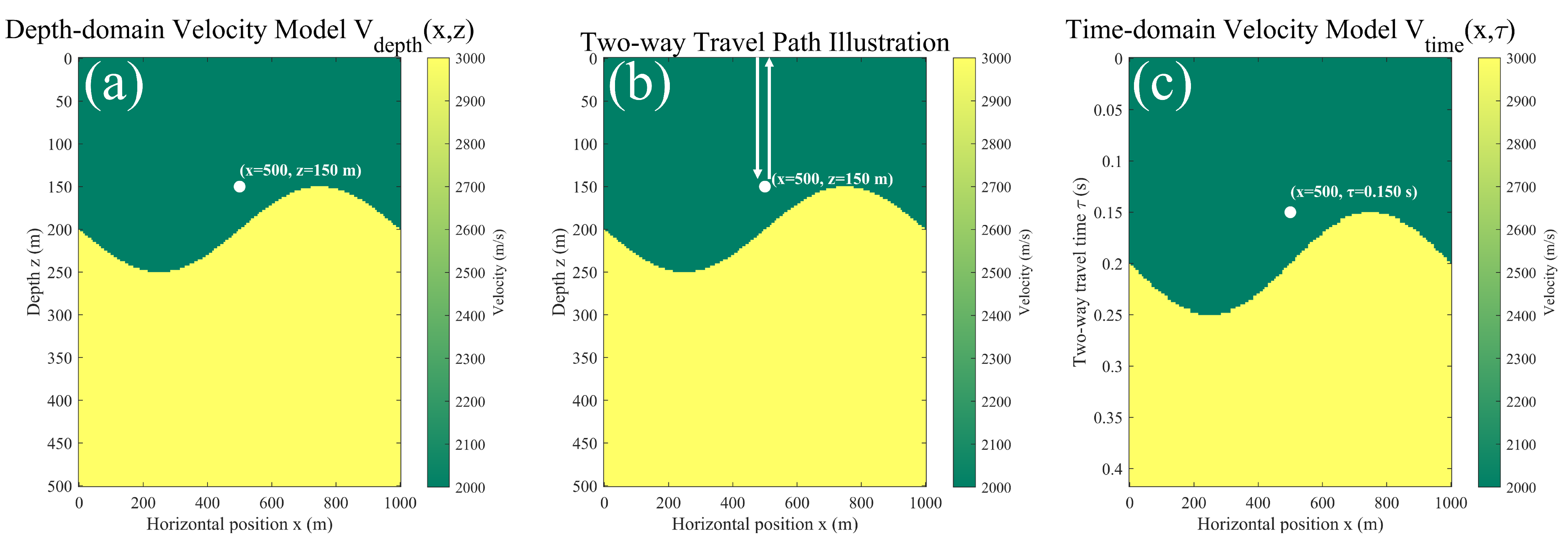
Therefore, for any given depth-domain velocity model ${\mathbf{V}}_{\mathrm{depth}}$, the corresponding time-domain velocity model ${\mathbf{V}}_{\mathrm{time}}$ can be obtained according to the above time–depth conversion relationship. Figure 1 illustrates the process by which subsurface points are mapped from the depth domain to the time domain.

Since the wavefield and the depth-domain velocity model can be linked through the wave equation, it can be mathematically inferred that a potential functional relationship also exists between the wavefield and the time-domain velocity model. The advantage of deep learning lies in its capability to approximate such complex nonlinear mappings in a data-driven manner without the need for explicit analytical formulations. Based on this concept, our research objective is transformed into learning the mapping from seismic records $\mathbf{D}$ to the time-domain velocity model ${\mathbf{V}}_{\mathrm{time}}$, namely,

$$\mathbf{D}\to {\mathbf{V}}_{\mathrm{time}}.$$

(7)

This idea is also inspired by conventional seismic data processing workflows, where time-domain sections are typically obtained as intermediate results. Therefore, directly predicting the time-domain velocity model from seismic data is not only physically reasonable but also consistent with the logical sequence of data processing in seismic exploration practice.

2.2. Deep Learning Method for Time-Domain Velocity Modeling Based on U-Net Architecture

In the proposed deep learning strategy, the model input consists of multi-shot seismic records $\mathbf{D}\in {\mathbb{R}}^{C\times H\times W}$, where W denotes the number of receivers, H represents the number of temporal sampling points, and C is the number of shot gathers. The model output corresponds to the time-domain velocity field $\mathbf{V}\in {\mathbb{R}}^{h\times w}$, where h indicates the temporal depth of the time-domain velocity model and w its lateral spatial extent.

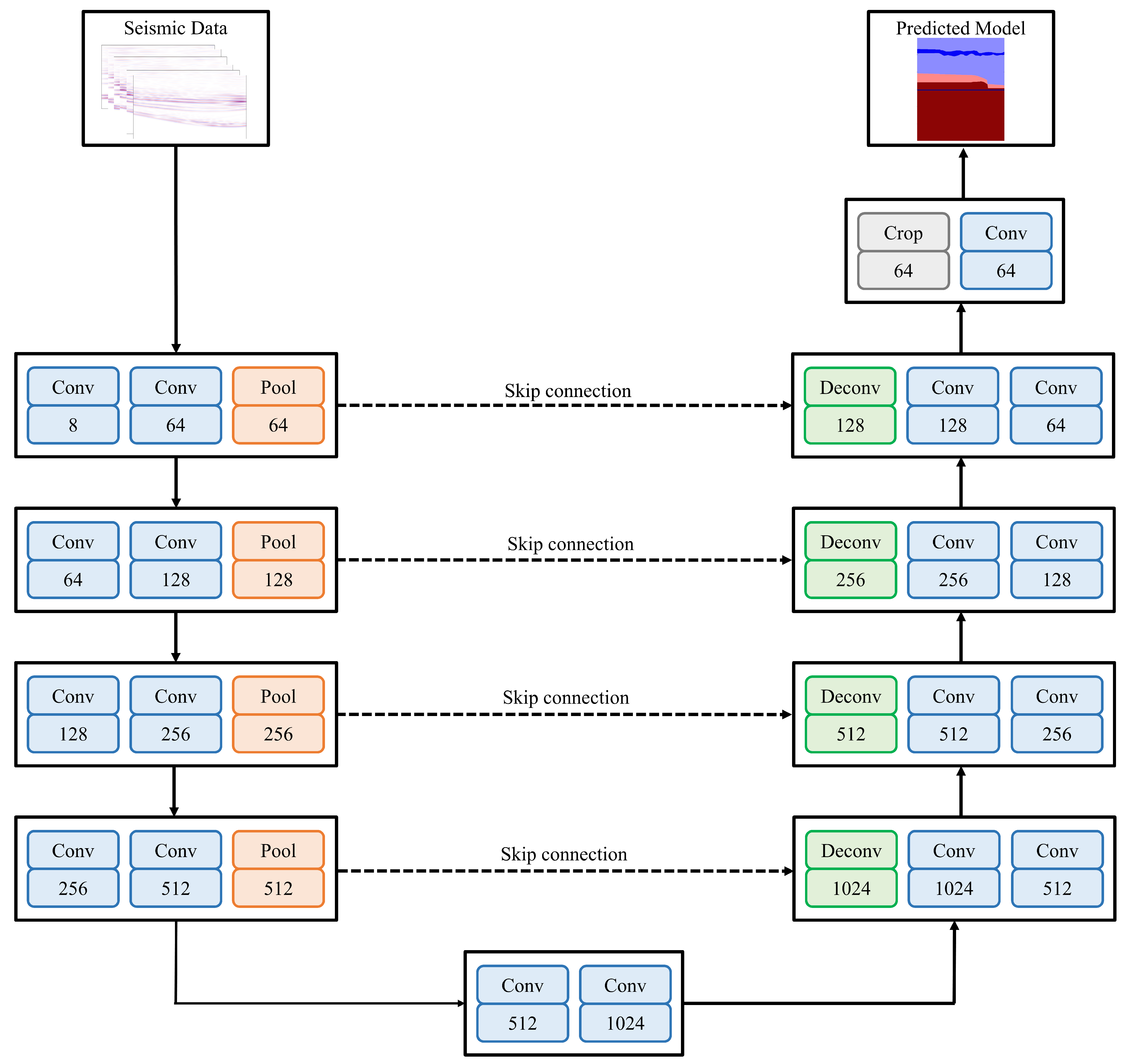
The neural architecture employed in this study is the U-Net network [40], as illustrated in Figure 2. Owing to its symmetric encoder–decoder structure, U-Net effectively fuses multi-scale features while preserving spatial resolution, making it particularly suitable for seismic velocity modeling and other inversion tasks characterized by strong spatial dependencies. The U-Net consists of three major components: a downsampling encoder, a central feature extraction block, and an upsampling decoder. The network takes the multi-shot seismic records $\mathbf{D}\in {\mathbb{R}}^{C\times H\times W}$ as input and outputs the corresponding time-domain velocity field $\mathbf{V}\in {\mathbb{R}}^{h\times w}$.

The encoder is composed of four downsampling blocks. Each block contains two $3\times 3$ convolutional layers followed by batch normalization and ReLU activation, and applies a $2\times 2$ max-pooling operation to perform downsampling. During this process, the network progressively extracts local spatial features and high-level semantic information from the seismic records, thereby expanding the receptive field. The number of feature channels increases successively as 64, 128, 256, and 512.

Following the encoder, a feature extraction layer further integrates global contextual information. This part adopts a double-convolution structure with 1024 channels, designed to capture deep-level propagation characteristics of seismic waves and the corresponding velocity variation patterns of the subsurface medium.

The decoder consists of four upsampling modules. Each module first applies a transposed convolution to restore spatial resolution and then concatenates the resulting feature maps with those from the corresponding encoder layer via skip connections, enabling the fusion of shallow spatial details with deep semantic features. The concatenated features are subsequently refined through two convolutional layers and non-linear activation to reconstruct detailed representations. This design allows the network to recover the spatial resolution of the velocity field while preserving critical structural features such as layer interfaces and velocity boundaries.

After multiple decoding and feature fusion stages, the output of the final upsampling layer is mapped to the target dimension through a $1\times 1$ convolution, generating the predicted time-domain velocity model ${\widehat{\mathbf{V}}}_{\mathrm{pred}}$.

In this study, the mean squared error (MSE) is employed as the optimization objective, owing to its stability, interpretability, and consistency with most existing deep learning-based velocity inversion frameworks. This choice allows for a fair evaluation of the proposed time-domain modeling strategy without the interference of additional hybrid or physics-informed constraints, defined as follows:

$$L\left(\theta \right)={\displaystyle \frac{1}{N}}\sum _{i=1}^N\left[{\displaystyle \frac{1}{h_i{w}_i}}\sum _{x=1}^{h_i}\sum _{y=1}^{w_i}{\left({\widehat{v}}_i(x,y)-v_i^{\mathrm{true}}(x,y)\right)}^2\right]$$

(8)

Here, $\theta$ denotes the set of network model parameters, N represents the total number of training samples, ${\widehat{\mathbf{V}}}_i=f_{\theta }\left({\mathbf{D}}_i\right)$ denotes the predicted velocity model for the i-th sample, and ${\mathbf{V}}_i^{\mathrm{true}}$ is its corresponding ground-truth velocity model. Specifically, ${\widehat{v}}_i(x,y)$ and $v_i^{\mathrm{true}}(x,y)$ are the velocity values at the spatial position $(x,y)$ of ${\widehat{\mathbf{V}}}_i$ and ${\mathbf{V}}_i^{\mathrm{true}}$, respectively. The variables $h_i$ and $w_i$ refer to the height and width of the i-th velocity field, respectively.

Considering the limitations of GPU memory and computational efficiency, a mini-batch training strategy is adopted. Under this setting, the loss function is reformulated as:

$$L\left(\theta \right)={\displaystyle \frac{1}{B}}\sum _{i=1}^B\left[{\displaystyle \frac{1}{h_i{w}_i}}\sum _{x=1}^{h_i}\sum _{y=1}^{w_i}{\left({\widehat{v}}_i(x,y)-v_i^{\mathrm{true}}(x,y)\right)}^2\right]$$

(9)

where B denotes the batch size, i.e., the number of samples processed per iteration.

During optimization, the network parameters $\theta$ are iteratively updated using a gradient-based optimization algorithm according to the following update rule:

$${\theta }_{t+1}={\theta }_t-\eta {\nabla }_{\theta }L\left({\theta }_t\right)$$

(10)

where $\eta$ represents the learning rate, and ${\nabla }_{\theta }L\left({\theta }_t\right)$ denotes the gradient of the loss function with respect to the model parameters at iteration t. Through iterative optimization, the network gradually learns the nonlinear mapping between the seismic records and the corresponding time-domain velocity fields until convergence to an optimal parameter configuration, thereby achieving accurate prediction of time-domain velocity structures.

In the testing phase, the trained model utilizes the optimized parameters ${\theta }^{\ast }$ to perform inference on unseen seismic data. Given a test seismic record ${\mathbf{D}}_{\mathrm{test}}$, the corresponding time-domain velocity field is obtained via forward propagation as:

$${\mathbf{V}}_{\mathrm{test}}=f_{{\theta }^{\ast }}\left({\mathbf{D}}_{\mathrm{test}}\right)$$

(11)

where $f_{{\theta }^{\ast }}$ denotes the trained neural network model, and ${\mathbf{V}}_{\mathrm{test}}$ represents the predicted time-domain velocity field.

3. Results

In this section, the proposed time-domain velocity modeling method is applied to the construction of aquifer velocity models. First, a dataset of aquifer velocity models was established based on typical stratigraphic characteristics, and multi-shot seismic records were generated through forward modeling using the acoustic wave equation. The resulting seismic records, together with the corresponding time-domain velocity models, constitute paired datasets required for network training, providing the foundation for subsequent deep learning-based modeling. To assess the effectiveness of the proposed approach, the predicted time-domain velocity fields were further transformed into the depth domain via time–depth conversion, yielding the corresponding depth-domain velocity models. A comparative analysis was then conducted against conventional end-to-end depth-domain velocity modeling methods. Experimental results demonstrate that the proposed time-domain end-to-end learning strategy achieves higher accuracy and robustness in identifying aquifer structures and recovering velocity distributions, particularly exhibiting enhanced resolution in regions with interlayer velocity discontinuities and aquifer boundaries. All experiments in this study were performed under the Windows operating system, and both training and inference were implemented using the PyTorch 2.9.0 deep learning framework [41]. The hardware configuration includes an NVIDIA GeForce RTX 5080 GPU (NVIDIA, Santa Clara, CA, USA) and an Intel(R) Core(TM) i5-14600KF CPU (Intel, Santa Clara, CA, USA).

3.1. Dataset Construction

This study constructed a representative dataset of depth-domain velocity models incorporating aquifers. The dataset comprises 2200 samples, each simulating typical multilayer geological structures, with the number of layers (including aquifers) ranging from 8 to 10. The velocity values within the models are set between 1500 m/s and 5000 m/s, covering the typical geophysical velocity variations from shallow sediments to deep bedrock. Each depth-domain velocity model has a grid size of $200\times 300$, with both horizontal and vertical spatial sampling intervals of 10 m, corresponding to a physical extent of 2000 m × 3000 m.

Based on these depth-domain models, the time–depth conversion was applied to generate the corresponding time-domain velocity models, yielding a dataset of 2200 time-domain samples. The converted time-domain velocity models have a uniform grid size of $834\times 300$, with the horizontal spatial sampling interval maintained at 10 m, and a temporal sampling interval of 0.002 s in the time–depth direction. This results in an actual physical extent of 1.668 s × 3000 m for the time-domain velocity models. Ten representative samples of the depth-domain aquifer velocity models and their corresponding time-domain velocity models are shown in Figure 3 and Figure 4, respectively.

In this study, forward numerical simulations were performed based on the depth-domain velocity models using the constant-density acoustic wave equation, generating seismic records corresponding to the time-domain velocity modeling task. The partial differential equation was discretized using a staggered-grid finite-difference scheme [42] to ensure numerical stability and accuracy of wavefield propagation. To effectively suppress boundary reflections affecting the simulated wavefield, a perfectly matched layer (PML) [43] was implemented as the absorbing boundary condition.

As the forward modeling is based on depth-domain velocity models, whereas the labels required for network training are time-domain velocity models, discrepancies exist in spatial scale and sampling dimensions. Upon conversion to the time domain, the time axis of the depth-domain velocity model undergoes nonlinear scaling according to local velocity variations, resulting in inconsistent sizes among different time-domain samples. To achieve uniform input dimensions while preserving physical fidelity, an extension of 100 grid points was applied to the bottom of the depth-domain velocity models during forward simulation in addition to the absorbing boundary, providing a sufficient buffer zone. This strategy ensures the integrity of wave propagation, maintains physically reasonable energy attenuation, and reduces numerical errors arising from time–depth conversion and boundary truncation.

Regarding temporal discretization, the simulation employed a time step of 0.4 ms and a sampling interval of 2 ms, with a total duration of 2 s, sufficiently covering the main wave propagation time while maintaining numerical stability. For the observation system, 8 sources and 301 receivers were evenly distributed at the surface, forming a multi-shot, multi-receiver acquisition geometry to obtain seismic records with high coverage, providing abundant spatiotemporal constraints for network training. An example of 8-shot seismic records corresponding to a single velocity model is shown in Figure 5.

3.2. Velocity Modeling of Aquifer Structures

A total of 2200 aquifer velocity model samples were partitioned into training, validation, and test sets at a ratio of 9:1:1, ensuring sufficient data diversity during model training while enabling effective evaluation of generalization performance. Prior to training, all data were normalized to enhance numerical stability and convergence, whereas no additional data augmentation strategies were applied. The optimization of network parameters was performed using the adaptive moment estimation (Adam) algorithm [44], with a learning rate of 0.001. The network was trained for 100 epochs using mini-batch stochastic gradient descent with a batch size of 5 [45] for parameter updates.

To prevent overfitting, the convergence of the model was dynamically monitored based on validation set performance, and the optimal network parameters were saved when the validation loss reached its minimum [46]. The resulting optimal model was then used to predict the time-domain aquifer velocity fields from the test set seismic records. Furthermore, we verified the robustness of the model across multiple random initializations, and the performance variations were minimal, indicating the stability and reliability of the proposed approach. Regarding the representativeness and diversity of the simulated dataset, the aquifer models were generated with random variations in the number of layers and velocity values (including those of non-aquifer layers). In addition, training samples were randomly selected during the training process to ensure adequate diversity and representativeness of the dataset. Representative results are shown in Figure 6, where panels (a)–(e) depict the true time-domain velocity fields and panels (f)–(j) show the corresponding predictions. The figure indicates that the model achieves high accuracy and consistency in reconstructing time-domain velocity fields, accurately recovering the spatial distribution and velocity characteristics of the aquifer. Moreover, the structures and velocity distributions of other geological layers are well reproduced, demonstrating the effectiveness of the proposed time-domain velocity modeling strategy.

To comprehensively assess the performance of the proposed time-domain aquifer velocity field modeling strategy relative to depth-domain modeling methods, a systematic comparative analysis was conducted from multiple perspectives. Specifically, the convergence processes of the loss functions during the training phase, including both training and validation loss curves, were compared to evaluate the learning stability and generalization capability of the models. In the testing phase, the predicted time-domain velocity fields were converted to depth-domain representations and compared with the true depth-domain velocity models in terms of spatial structures and velocity distributions, using both qualitative image comparison and quantitative error analysis. Furthermore, forward simulations and reflection coefficient calculations based on the predicted velocity fields were performed to verify the physical plausibility and accuracy of the model in reconstructing seismic wave propagation characteristics and interface responses. Taken together, these multi-dimensional analyses effectively validate the rationality and superiority of the proposed time-domain velocity field modeling strategy.

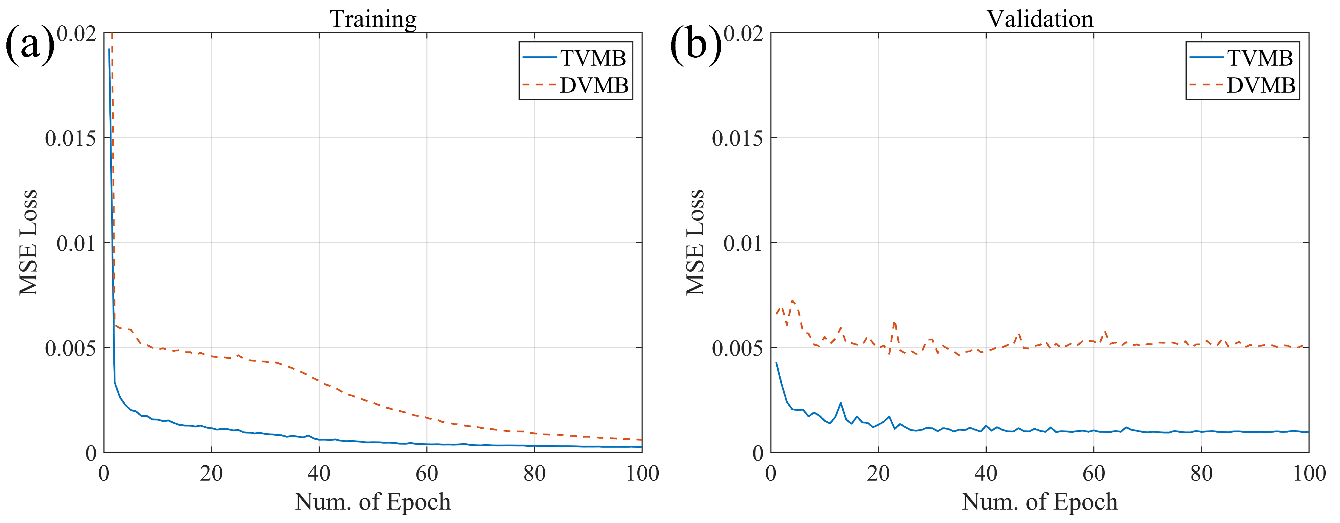
The loss convergence during training and validation is shown in Figure 7. Panel (a) presents the mean squared error (MSE) loss curve for the training set, while panel (b) shows the MSE loss curve for the validation set. It is evident that, in both training and validation phases, the time-domain velocity modeling strategy exhibits faster convergence and lower final loss values, demonstrating a clear advantage over the depth-domain modeling strategy. Specifically, the loss function of TVMB decreases rapidly during early iterations and stabilizes, indicating that the model can more efficiently learn the mapping between seismic records and velocity fields in the time domain. In contrast, DVMB converges more slowly and exhibits larger fluctuations on the validation set, reflecting weaker generalization performance. Overall, the time-domain modeling strategy outperforms the depth-domain approach in terms of stability and convergence, validating its advantages in training efficiency and model fitting capability.

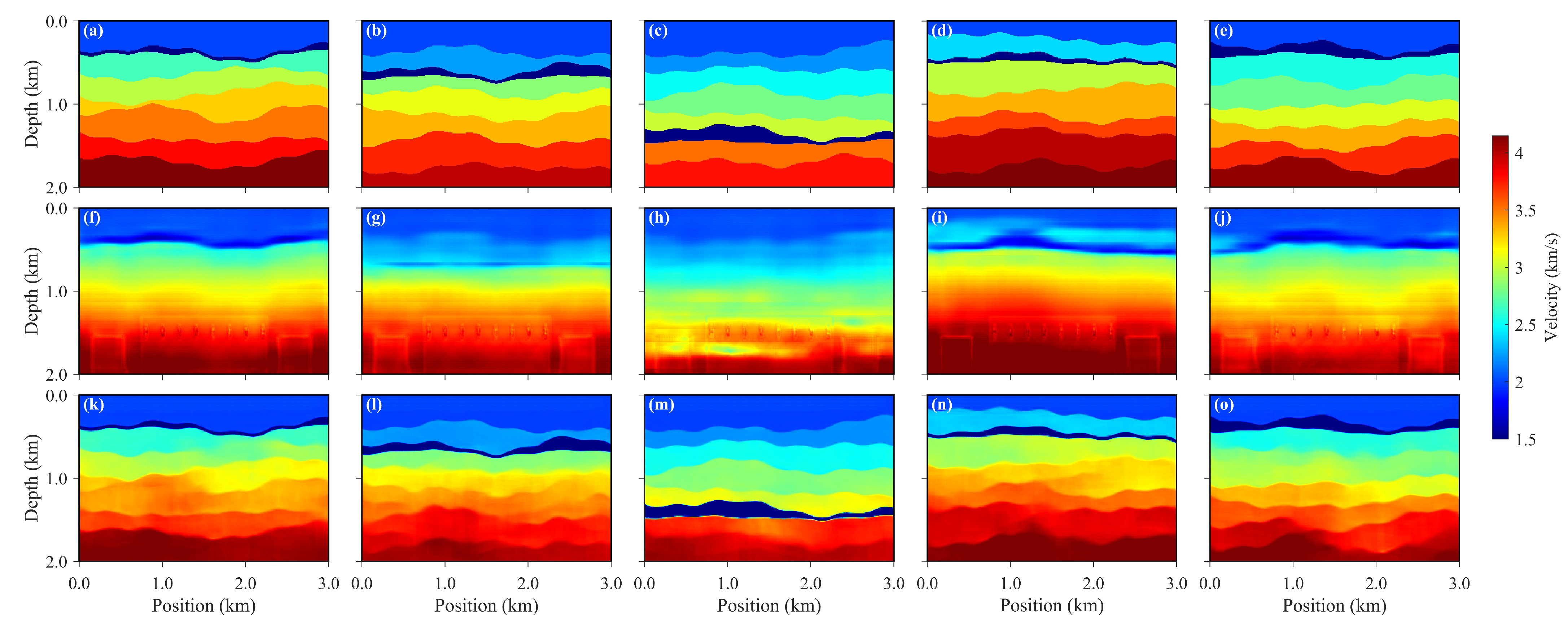
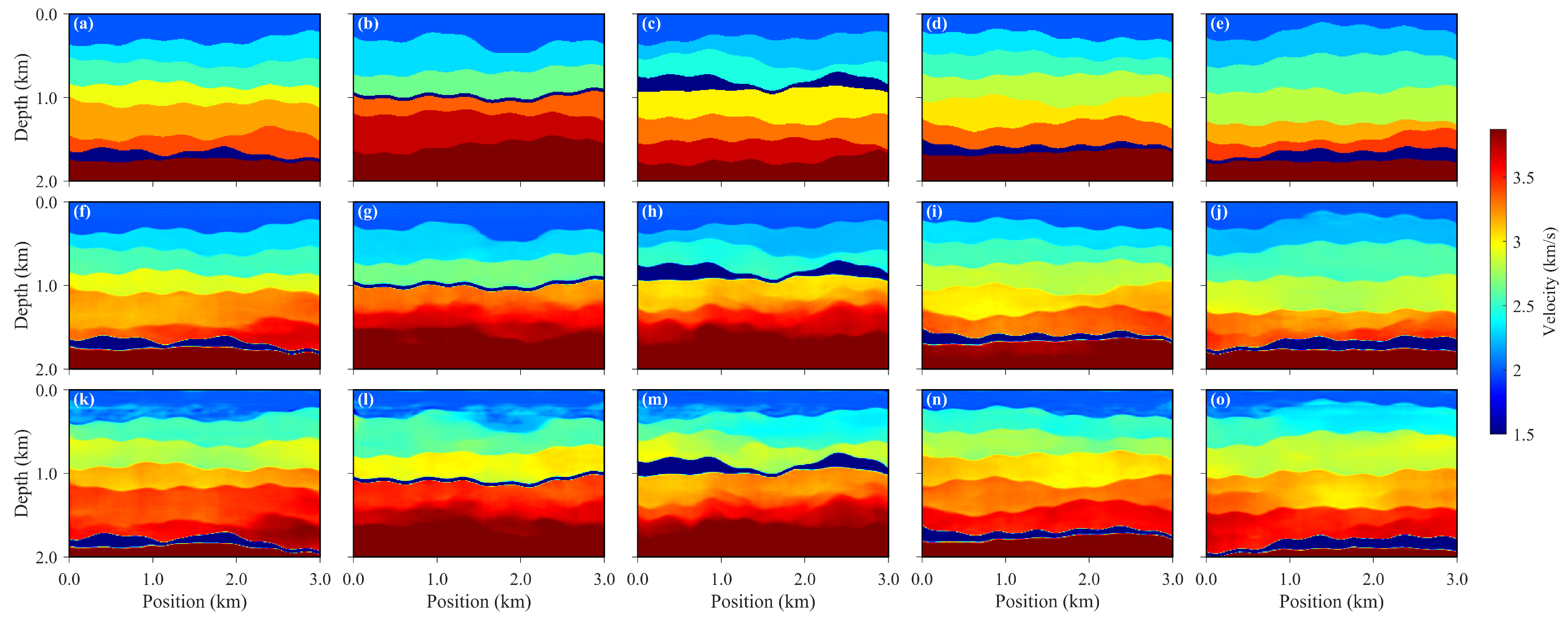
The velocity field predictions obtained using different methods are shown in Figure 8, where panels (a)–(e) correspond to the true velocity models, panels (f)–(j) show the predictions based on the depth-domain modeling strategy, and panels (k)–(o) present the results of the time-domain modeling strategy converted to the depth domain. It is evident that the TVMB approach outperforms DVMB in terms of the accuracy of velocity layer interfaces, interlayer velocity gradients, and the reconstruction of aquifer geometries. Specifically, TVMB more precisely restores the detailed features in regions of velocity discontinuity, producing smoother transitions between layers that are consistent with geological continuity, whereas the DVMB results exhibit some interface blurring and velocity deviations. Moreover, the TVMB predictions demonstrate higher overall and local consistency with the true velocity fields, indicating that the time-domain modeling strategy possesses stronger capability in capturing the dynamic relationships of the velocity field with improved physical fidelity. Overall, the results suggest that the time-domain velocity modeling method significantly surpasses the depth-domain approach in both inversion accuracy and preservation of geological structures.

The quantitative evaluation metrics of predictions obtained using different methods are summarized in

Table 1. Quantitative comparison of prediction results obtained using different methods.

Method	MSE ($\times {10}^{-3}$)	PSNR	SSIM
DVMB	4.26	24.59	0.66
TVMB (time domain)	0.91	30.93	0.91
TVMB (depth domain)	1.48	28.96	0.88

. Table 1 reports the MSE, peak signal-to-noise ratio (PSNR), and structural similarity index (SSIM) [47] over 200 test samples for the depth-domain velocity modeling, the time-domain velocity modeling, and the TVMB results converted back to the depth domain. It can be observed that the TVMB method outperforms DVMB across all three metrics. Specifically, the MSE of TVMB is substantially lower than that of DVMB, indicating a closer match to the true velocity fields. The PSNR and SSIM of TVMB reach 30.93 and 0.91, respectively, which are significantly higher than those of DVMB (24.59 and 0.66), demonstrating that time-domain velocity modeling achieves both higher reconstruction quality and structural consistency. Furthermore, when the TVMB results are converted to the depth domain, the metrics remain high (MSE = $1.48\times {10}^{-3}$, PSNR = 28.96, SSIM = 0.88), further validating the advantages of the time-domain strategy in cross-domain consistency and physical plausibility. These results collectively indicate that time-domain modeling not only improves the accuracy and stability of velocity inversion but also maintains good transferability and consistency across domains. The PSNR and SSIM are computed as follows:

$$\mathrm{PSNR}=10·{log}_{10}\left({\displaystyle \frac{V_{max}^2}{\mathrm{MSE}(p,g)}}\right)$$

(12)

$$\mathrm{SSIM}(g,p)={\displaystyle \frac{(2{\mu }_g{\mu }_p+C_1)(2{\sigma }_{gp}+C_2)}{({\mu }_g^2+{\mu }_p^2+C_1)({\sigma }_g^2+{\sigma }_p^2+C_2)}}$$

(13)

where g and p denote the true and predicted velocity fields, $V_{max}$ is the maximum possible velocity value, ${\mu }_g$ and ${\mu }_p$ are the means of g and p, ${\sigma }_g$ and ${\sigma }_p$ are the variances of g and p, ${\sigma }_{gp}$ is the covariance between g and p, and $C_1$, $C_2$ are constants added to avoid division by zero.

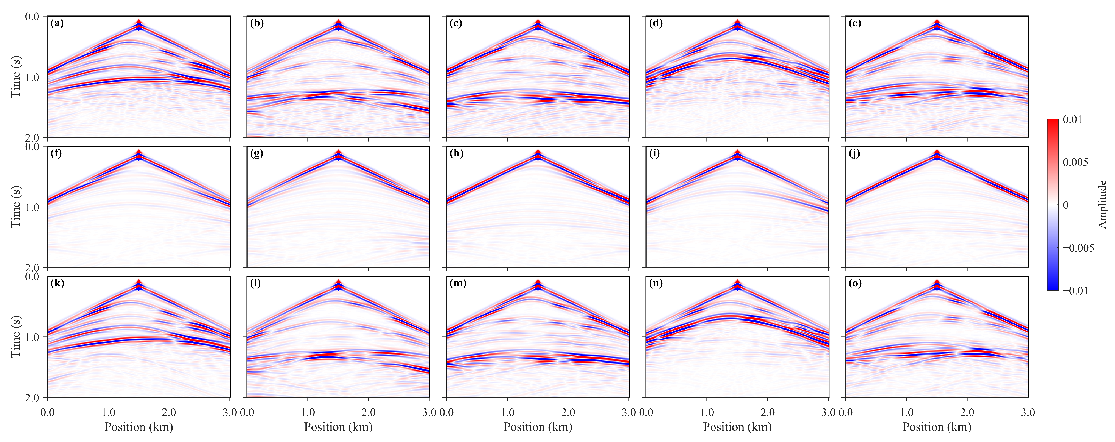
The forward-modeled seismic records corresponding to the predicted velocity fields obtained using different methods are shown in Figure 9. Panels (a)–(e) present the forward records generated from the true velocity fields, panels (f)–(j) correspond to the forward records based on predictions from the depth-domain velocity modeling method, and panels (k)–(o) represent the forward records derived from the time-domain velocity modeling results after conversion to the depth domain. It can be clearly observed that the forward records generated by TVMB closely resemble the true seismic records in terms of waveform shapes, amplitude characteristics, and event continuity. In contrast, the DVMB-derived forward records exhibit deviations in energy distribution along the same phase axes and in phase characteristics, indicating that the predicted velocity fields do not fully capture the detailed variations of the subsurface medium. In particular, at the aquifer and its adjacent layer interfaces, the velocity structures predicted by the TVMB model yield clearer and better-aligned reflection events, demonstrating stronger physical consistency and representational capability in preserving wave propagation dynamics and reconstructing reflective interfaces. Collectively, these forward modeling results provide further evidence of the effectiveness and physical plausibility of the time-domain velocity modeling strategy, showing that its predictions not only outperform the depth-domain approach in quantitative metrics but also better reproduce the seismic response in terms of wavefield propagation features.

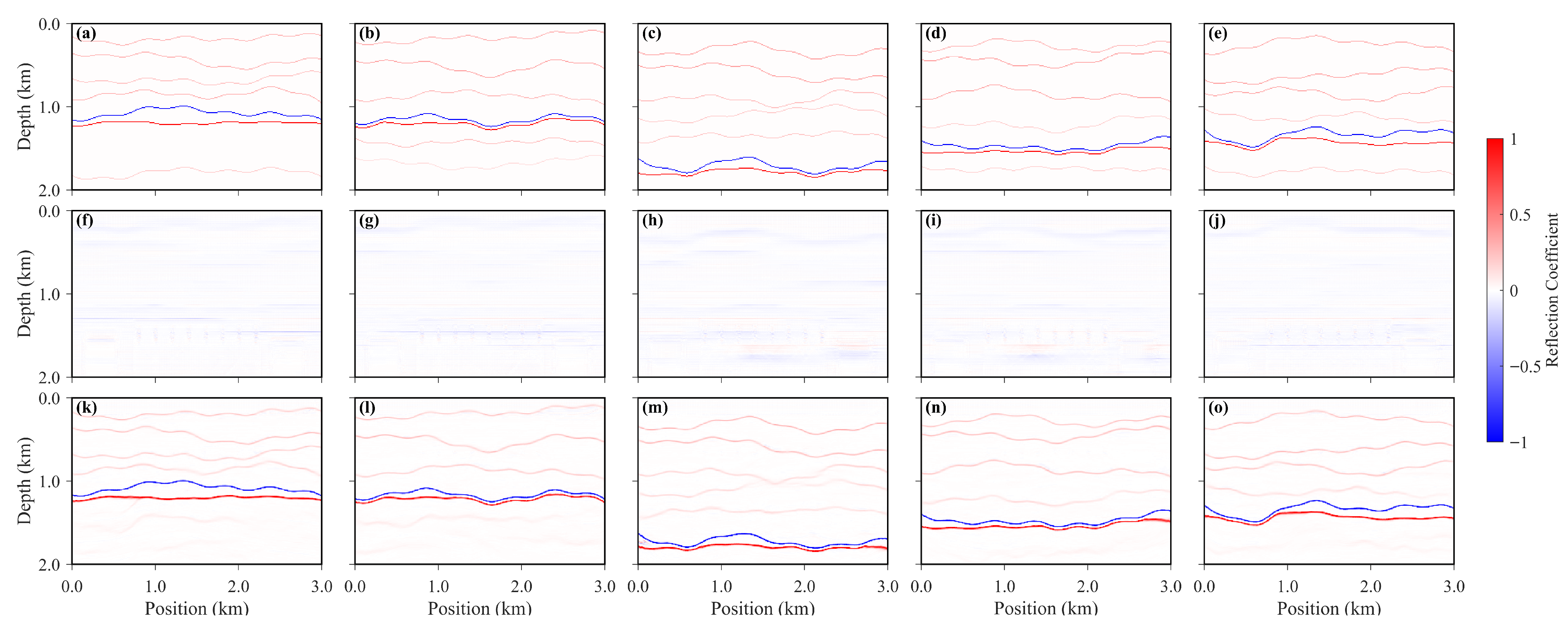
The reflection coefficients computed from the velocity fields predicted by different methods are shown in Figure 10, where panels (a)–(e) correspond to the true reflection coefficient profiles, panels (f)–(j) represent the reflection coefficients derived from the DVMB predictions, and panels (k)–(o) show the reflection coefficients obtained from the TVMB results after conversion to the depth domain. It can be clearly observed that the reflection coefficients calculated from the TVMB velocity fields, after conversion to the depth domain, exhibit a higher degree of consistency with the true profiles in terms of the spatial distribution of reflection interfaces, amplitude variations, and inter-layer reflection details. Specifically, the TVMB-derived profiles preserve the lateral continuity of strong reflection interfaces and accurately capture the details of weakly reflective layers, whereas the DVMB-derived profiles show certain deviations in interface accuracy and detail reconstruction. These observations indicate that the TVMB approach achieves superior precision in constructing depth-domain velocity fields and subsequent reflection coefficient computation, more accurately reflecting the reflective characteristics of the subsurface medium. In this study, the reflection coefficient under the constant-density assumption is expressed as follows:

$$R={\displaystyle \frac{V_2-V_1}{V_2+V_1}}$$

(14)

where R denotes the reflection coefficient at the interface, and $V_1$ and $V_2$ represent the P-wave velocities of the upper and lower media, respectively. The formulation is derived under the assumption of normal incidence and equal densities on both sides of the interface (${\rho }_1={\rho }_2$). Under these conditions, the reflection coefficient is governed solely by the discontinuity in P-wave velocity and can be used to quantitatively characterize the amplitude and polarity of seismic reflections generated at velocity-contrast interfaces.

4. Discussion

To further assess the robustness and applicability of the proposed time-domain velocity modeling approach, systematic tests and analyses were conducted to evaluate its noise resilience and the influence of the number of input seismic sources on network training performance. By introducing controlled noise into the seismic records and training and validating the model under different source configurations, the generalization capability of the time-domain modeling strategy in complex, low signal-to-noise seismic environments was examined, as well as its sensitivity to variations in observational coverage. These investigations provide a comprehensive evaluation of the method’s stability and reliability for practical seismic exploration applications.

4.1. Noise-Resilience Evaluation

To evaluate the robustness of the trained model under noisy conditions, Gaussian noise with zero mean and a standard deviation of 0.003 was added to the seismic records in the test set. Subsequently, predictions were performed using the network model trained without noise-robust strategies, in order to analyze the impact of noise on the inversion results. An example of a multi-shot noisy seismic record is shown in Figure 11, and the corresponding predicted velocity field is presented in Figure 12.

As observed in Figure 12, the addition of noise has a noticeable effect on the predicted results. Compared with the noise-free condition, the predicted velocity fields exhibit deviations in amplitude, layer interface morphology, and position, while overall resolution and interlayer transition characteristics are reduced. In particular, regions with large velocity gradients show weakened detail recovery due to noise interference. Nevertheless, the overall geological structure and velocity distribution are largely preserved, indicating a certain degree of noise resilience.

Quantitative evaluation results are listed in

Table 2. Quantitative comparison of the impact of noise on prediction results.

Method	MSE ($\times {10}^{-3}$)	PSNR	SSIM
TVMB (time domain, noise-free seismic records)	0.91	30.93	0.91
TVMB (depth domain, noise-free seismic records)	1.48	28.96	0.88
TVMB (time domain, noisy seismic records)	2.10	27.31	0.90
TVMB (depth domain, noisy seismic records)	8.77	21.82	0.73

. It can be seen that in the time-domain velocity fields, the reductions in PSNR and SSIM are relatively moderate (PSNR decreased from 30.93 to 27.31, SSIM from 0.91 to 0.90), whereas after time-to-depth conversion, the metrics decline more substantially (PSNR from 28.96 to 21.82, SSIM from 0.88 to 0.73). This indicates that the cumulative effect of noise is amplified through the time-to-depth transformation, leading to a significant deterioration of the depth-domain velocity field quality.

In summary, the introduction of noise has a considerable impact on seismic-record-based velocity modeling, particularly in the depth domain. However, the model retains the overall plausibility of the velocity structure under complex noise conditions, demonstrating its generalization ability and noise-robustness.

4.2. Effect of Different Source-Array Configurations on Model Training Results

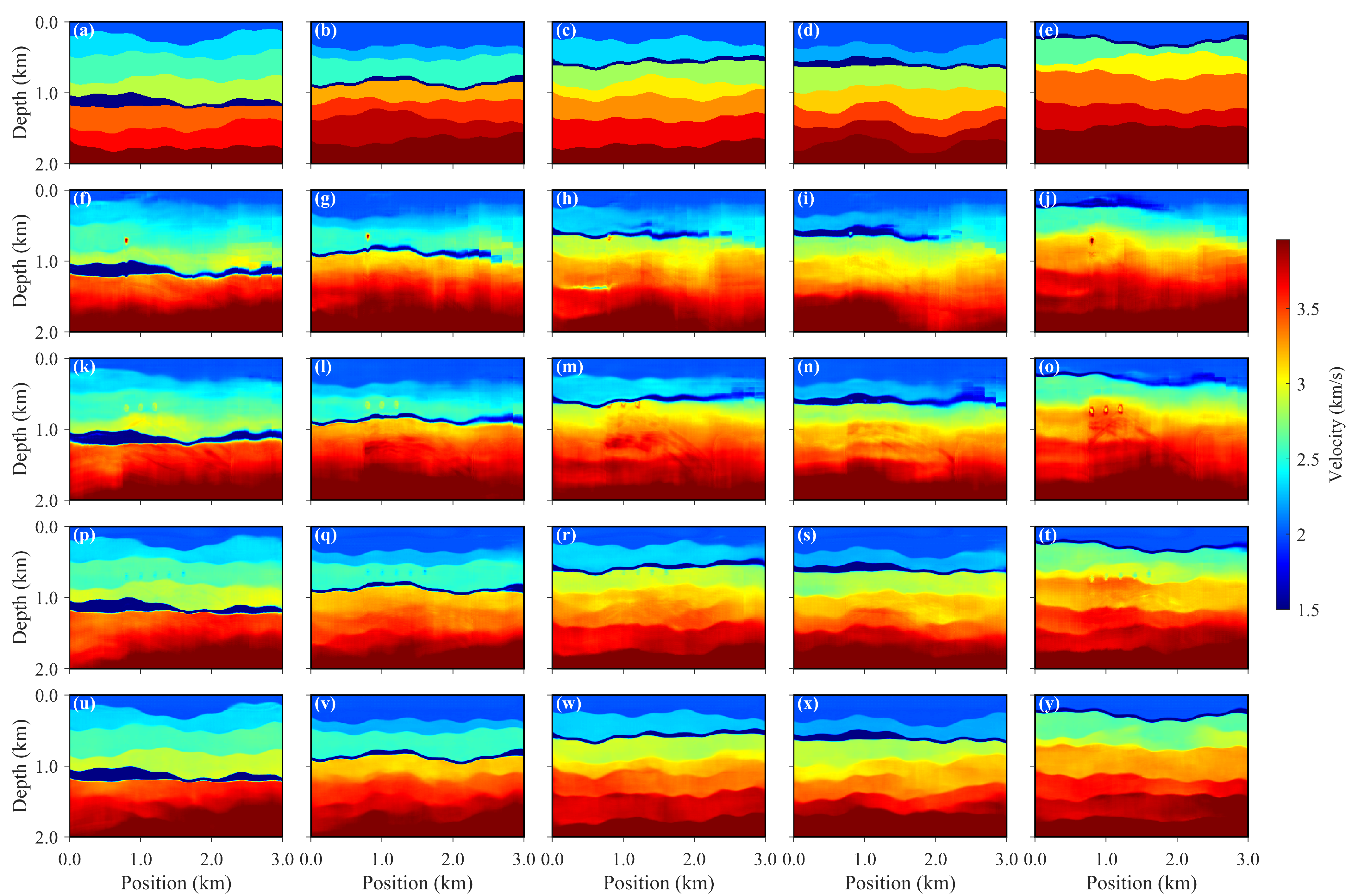
To investigate the influence of the number of input seismic shots on the network inversion results, a series of systematic comparative experiments were conducted. Specifically, seismic records corresponding to 1, 3, 5, and 8 shots were respectively selected as inputs, and independent training was performed for each configuration. To ensure comparability and scientific rigor, all models were trained using identical dataset partitions, network architectures, and training parameter settings, and evaluated under the same testing conditions. By comparing the network predictions in the depth domain under different input shot numbers, the effect of multi-shot information on the inversion performance can be systematically analyzed.

Figure 13 presents the velocity fields in the depth domain predicted by the TVMB model under various shot-input conditions. It is evident from the figure that, as the number of input seismic records increases, the model’s ability to delineate subsurface velocity structures improves significantly. When only a single-shot record is used, the predicted stratigraphic interfaces appear blurred and the velocity distribution is discontinuous, indicating that single-shot data suffer from limited spatial coverage and weak constraint capability, leading to considerable uncertainty in the inversion results. In contrast, as the input shot number increases to 3, 5, and 8, the predicted velocity interfaces become progressively clearer, and the spatial distribution of the velocity field exhibits improved continuity and stratification. The model thus more accurately captures the lateral variations of the subsurface medium.

These observations demonstrate that the incorporation of multi-shot information effectively enhances the model’s perception and constraint capabilities for subsurface structures, compensating for the limitations of single-shot observations in spatial coverage and inversion uncertainty. The joint utilization of multi-shot data substantially improves both the spatial resolution and geological structure recognition of the network. Furthermore, quantitative evaluation results of the TVMB inversions under different shot-input conditions are summarized in

Table 3. Quantitative comparison of TVMB inversion results in the depth domain under different numbers of input seismic shots.

Method	MSE ($\times {10}^{-3}$)	PSNR	SSIM
TVMB (1 shot)	3.67	24.95	0.79
TVMB (3 shots)	3.12	25.71	0.80
TVMB (5 shots)	1.95	27.85	0.85
TVMB (8 shots)	1.48	28.96	0.88

. The metrics presented therein further substantiate the above findings. With the increase in the number of input shots, the model exhibits consistent improvements in MSE, PSNR, and SSIM, aligning well with the visual inspection results. This consistency indicates that the inclusion of multi-shot information significantly enhances both the accuracy and stability of deep-learning-based seismic inversion.

4.3. Future Work

Although this study has demonstrated the effectiveness and potential of the deep learning-based seismic time-domain velocity modeling method for aquifer velocity inversion, certain limitations remain. First, at the dataset level, the 2200 samples used in this study were primarily generated from idealized two-dimensional synthetic models based on the constant-density acoustic wave equation. While this design allows for controlled validation of methodological feasibility and systematic performance evaluation, the dataset size is limited, the geological diversity is insufficient, and the simulation approach is overly simplified, making it difficult to fully capture the complexity of real subsurface environments. In practice, seismic data are often affected by noise, heterogeneity, and irregular sampling, whereas the geological structures in the current dataset are relatively idealized and lack representations of complex stratigraphy, multi-phase sedimentation, and faulting features. To address these issues, future research will focus on improving the construction of the dataset by incorporating more representative field seismic data and integrating geological, well-logging, and geophysical constraints to enhance the model’s applicability and generalization in real-world scenarios. In addition, more realistic simulation methods, such as variable-density or elastic wave equation modeling, will be employed to improve the physical consistency and representativeness of the training data, providing a more reliable physical foundation for model development.

Moreover, the current modeling framework has been validated primarily on isotropic two-dimensional media. Although the two-dimensional experiments have confirmed the effectiveness and physical plausibility of the proposed time-domain modeling approach in aquifer structure identification and velocity field reconstruction, its scalability to three-dimensional scenarios and anisotropic geological conditions remains to be further explored. Future work will focus on extending the time-domain modeling framework to three-dimensional and anisotropic media, and on integrating physics-based constraints or hybrid inversion strategies to achieve more accurate modeling and high-dimensional velocity inversion in geologically complex environments.

In addition, as discussed in the “Noise-resilience Evaluation” section, experimental results indicate that the introduction of noise has a minor effect on the accuracy of time-domain velocity modeling. However, once the time-domain results are converted into the depth domain, the degradation in velocity modeling accuracy becomes much more pronounced. The root cause of this issue lies in error accumulation and nonlinear mapping distortion during the time-to-depth conversion process, which represents one of the key limitations of the current approach. Future work will focus on optimizing the time-to-depth conversion strategy or developing approaches that enable direct geological interpretation and constraint within the time-domain framework, thereby mitigating this limitation and further improving the accuracy and stability of time-domain velocity modeling.

5. Conclusions

This work proposes an end-to-end deep learning approach for directly mapping seismic records to time-domain velocity models, which is further applied to the inversion of aquifer velocities. Compared with conventional depth-domain modeling approaches, the method demonstrates significant advantages both theoretically and experimentally. The time-domain modeling strategy establishes a mapping between seismic records and velocity models within the same physical domain, ensuring that both the input and output reside in the time domain and thus remain physically consistent. Since seismic records inherently represent the temporal response of subsurface media to seismic wave propagation, and the time-domain velocity model likewise characterizes subsurface velocity variations as a function of time, this consistency allows the network to learn the correspondence between the two in a more natural and direct manner. Consequently, the inversion mapping becomes simpler, and the overall modeling process achieves greater stability and accuracy. Experimental results indicate that time-domain modeling achieves superior performance in aquifer structure identification, characterization of velocity gradients, and interface position reconstruction. The predicted velocity fields not only exhibit high spatial consistency with the true models but also display stronger physical plausibility in forward-modeled seismic responses and reflection characteristics. Furthermore, the method retains robust velocity structure reconstruction under noisy conditions and demonstrates improved generalization with an increasing number of seismic shots. Overall, the proposed time-domain deep learning modeling approach overcomes the limitations of traditional depth-domain methods, providing new avenues for high-resolution seismic velocity inversion and subsurface aquifer characterization, with significant theoretical and practical implications.