Interspace Minimisation for Optimal Description of Temperature-Dependent Nonlinear Material Behaviour

Abstract

This paper focuses on optimisation of material parameters to describe the elastoplastic stress–strain relationship in finite element solvers. Two new methods are introduced to minimise the numerical error that occurs in the interspace between the experimental cyclic stress–strain curve and its representation using multilinear interpolation. Specifically, both methods are integrated into a Prandtl operator approach, which can be used to simulate the elastoplastic response of mechanical components subjected to variable thermomechanical loadings. The improvement as compared to standard interpolation is most substantial when the number of yield planes is limited, especially in the case of bilinear stress–strain curves. The innovation of this study is an algorithm that optimises positions of the stress–strain points across the temperature range of interest considering several input temperatures. It is shown that these methods are especially applicable for optimisation of material parameters when the stress–strain curves are available for a range of test temperatures that are needed for simulating thermomechanical fatigue. The improvement in the interpolation using these methods is exhibited for two materials with available experimental results: stainless steel EN 1.4512 and polyamide PA12.

1. Introduction

The basis for product development often includes preliminary assessment of durability using numerical methods, amongst which finite element analysis (FEA) is extensively used. To include various material properties, commercial and open-source solvers use verified material models of different complexities to simulate their nonlinear material behaviour under cyclic loading. Choosing the right model can affect the accuracy of the results and significantly affect computational time. During their lifetime, mechanical components such as exhaust systems, internal combustion engines, power plants, etc., experience periods of thermomechanical cyclic loading [1,2,3,4,5,6]. Materials for components that are subjected to thermomechanical fatigue at elevated temperatures, which typically exceed 30–50% of the material melting temperature, can be simulated using material models that either include or neglect viscoplastic effects, i.e., creep and relaxation. Nevertheless, elastoplastic material properties must be considered regardless of the operational temperature. Typical material models in simulations include the Ramberg–Osgood model [7] to simulate the nonlinear stress–strain relationship or the Armstrong–Frederick nonlinear kinematic hardening model [8], which is often used to simulate hardening behaviour of metals with characteristic features, e.g., Bauschinger and ratcheting effects. The Johnson–Cook model [9,10] uses temperature-dependent yield stress and is used to predict material behaviour under demanding conditions of high stresses, strains and temperatures. The Anand constitutive model [11,12] is used for simulating elastic–viscoplastic strains at high temperatures and includes temperature-dependent grain size effects. The more complex Chaboche model [13] also includes changes in the yield surface of the material, which are used to model isotropic and kinematic hardening. As opposed to the Ramberg–Osgood model, which only needs a few material parameters freely available for widely used materials, the parameters for the Chaboche model are often unavailable and require additional testing. Some recent studies concerning either application of existing material models or proposal of new formulations in simulations have been presented by Lucchetta et al. [14], who suggested a double incremental variational formulation to investigate the behaviour of elastoplastic composites exhibiting both isotropic and nonlinear kinematic hardening, and Mirkoohi et al. [15], who proposed an analytical thermomechanical model to predict a thermal stress–strain relation in additive manufacturing. Nagode et al. [16] proposed a closed-form solution for the FEA and implemented the Prandtl model to allow for temperature-dependent stress–strain modelling with multilinear kinematic hardening and a Ramberg–Osgood-type description of the cyclic curve, as follows:

$$\epsilon =f(\sigma ,T)={\displaystyle \frac{\sigma }{E\left(T\right)}}+{\left({\displaystyle \frac{\sigma }{K^{\prime }\left(T\right)}}\right)}^{1/n^{\prime }\left(T\right)},$$

(1)

where E(T), $K’\left(T\right)$ and $n’\left(T\right)$ are the Young’s modulus, cyclic hardening coefficient and cyclic hardening exponent, respectively. These parameters can be obtained from the existing literature for a wide range of materials at various temperatures. For intermediate temperatures, the material parameters are usually obtained by linear interpolation. An important advantage of the Prandtl model is that in contrast to other models, the material parameters are calculated and stored prior to the simulations. This reduces the computational time of the simulations, as the material properties of the model are calculated only once and then used for an arbitrary number of simulations using that material. In comparison to the Besseling model [17], which is typically used for simulating a cyclic elastoplastic response with consideration of multilinear kinematic hardening, the Prandtl operator approach ensures up to 30% shorter computational times [16,18]. If other materials are considered, e.g., polymer materials such as PA12, the Prandtl model must be calibrated to represent the corresponding material properties. In FEA, the simulation times are dependent on the number of segments used for the multilinear representation of the cyclic curve. If the cyclic stress–strain curve interpolation is performed using the Prandtl model, the number of yield planes for the discretisation of the curve corresponds to the number of spring-slider segments on the model [16]. To reduce the interpolation error of the multilinear representation, either more yield planes can be used for the discretisation or the existing positions of the yield planes can be adjusted for a better curve fitting. Importantly, however, the increase in the number of discretisation points always also increases the simulation time of the FEA, so the latter option is preferable to reduce the interpolation error. Moreover, there are occasions where linear or bilinear curves to simulate the material behaviour are favoured [19,20,21].

It is often the case that a pragmatic approach for the determination of material parameters is utilised. This depends on the available test sample size and the type of tests provided. Here, a systematic approach for the determination of material parameters is presented, which can be used when repeated tests of the same type are available. Typically, materials that are used for high-temperature operations are tested under low cycle fatigue conditions and at a few distinct test temperatures. Such a systematic approach to testing can thus also benefit from a systematic approach to the determination of material parameters. In the area of determining optimal material properties, a few methods have been recently published, but none of them have focused on optimisation with respect to several test temperatures. Marković et al. [22] developed a recursive algorithm for the optimal interpolation point selection of a given stress–strain curve. McDonnell et al. [23] demonstrated a method to simulate a compressive stress–strain curve by using a genetic algorithm to optimise the design variables of lattice structures by minimising the error between the target stress–strain curve and predicted stress–strain curve. Pandey et al. [24] developed a new method to determine Ramberg–Osgood parameters using experimental data from various specimen types combined with FEA. Since the processing time required for optimising material parameters is typically not comparable to the time needed to carry out the numerical simulation—as the material parameter optimisation is performed only once—allocation of more processing time for optimisation can therefore be harmlessly afforded. Focusing on the material parameters of the Prandtl model, more complex and iterative schemes to reduce the interpolation error have therefore been investigated without increasing the amount of spring-slider segments. Recent studies [22,23,24] have focused on the interpolation of cyclic stress–strain curves for a single temperature. The main subject of this study is therefore a proposition of an algorithm that provides cyclic stress–strain curve interpolation with minimal error for various materials, but is particularly focused on optimisation with respect to several available input temperatures.

This paper is structured as follows. The algorithm is first introduced in detail in Section 2. Next, it is validated for ferritic stainless steel EN 1.4512, and finally, it is applied to the test results of the polymer material PA12. The results of the interpolation methods and assessment criteria are discussed in Section 3 and Section 4.

2. Method

Using Equation (1), the cyclic curve using the Ramberg–Osgood relation can be obtained (black line in Figure 1a–c). On the contrary, the multilinear material models used in FEA use an approximation of this curve (blue lines in Figure 1a–c). Considering the Prandtl model, the distinction between two linearised curves depends on the positions of the yield planes. This can be clearly seen when changing from four yield planes in Figure 1a to seven yield planes in Figure 1b as the multilinear description of the Ramberg–Osgood equation becomes smoother. When interpolating a stress–strain curve, linear interpolation gives the largest error in regions where the slope of the curve changes significantly. By using an algorithm that increases the number of yield planes in areas with intense slope variations, the numerical error can be reduced. Inversely, as also seen in Figure 1a between the first and the second yield plane, reducing the number of yield planes in regions that resemble a linear function does not significantly increase the error. Laug and Borouchaki [25] therefore presented a curve discretisation method that builds a polyline that approximates the given curve with consideration of the curve radius. The same algorithm is also used in this study to find the values of the yield planes, as shown in Figure 1.

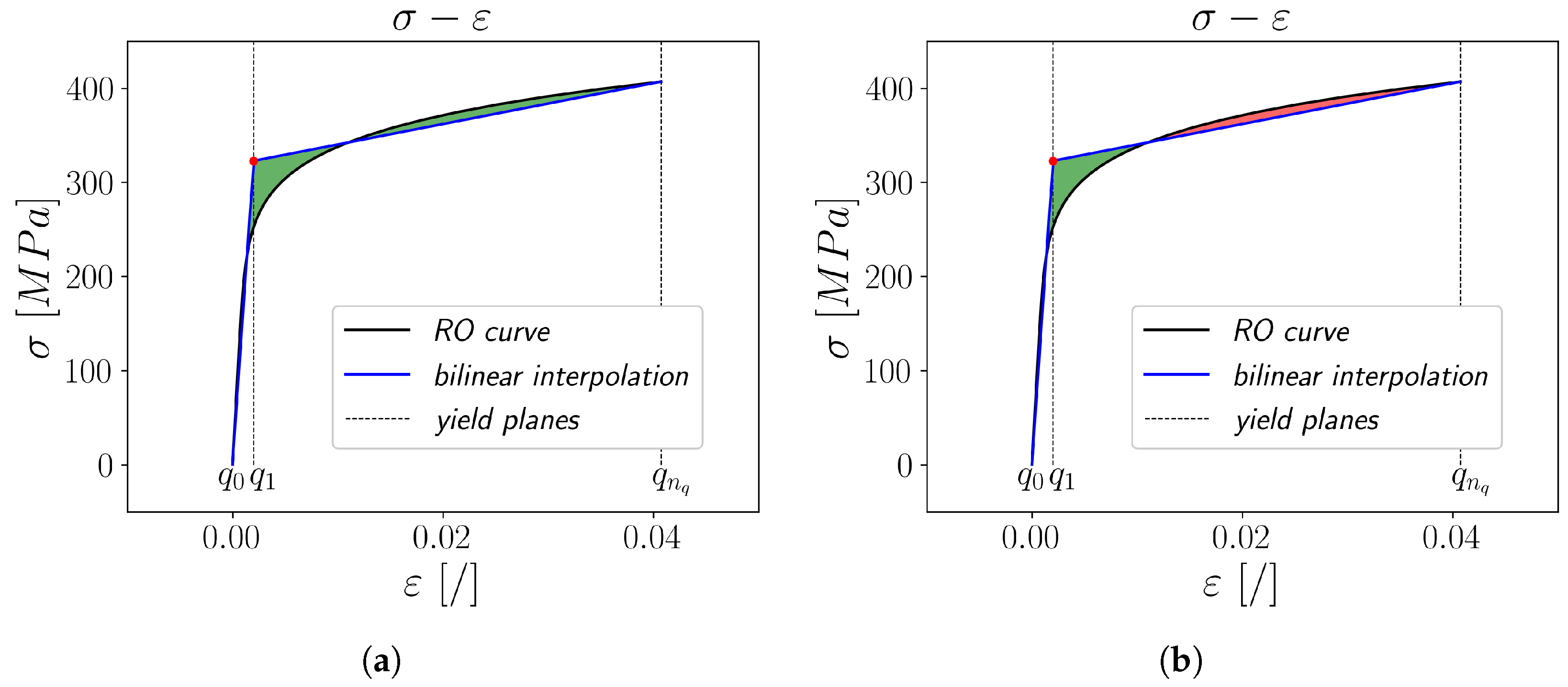
Conventional curve discretisation methods are based on the assumption that the discretisation points lie on the actual cyclic stress–strain curve. When applying this assumption to linear interpolation, the energy required for material fracture along the interpolated curve will always be lower than the actual value. To reduce this error without increasing the amount of yield planes, some of these have to be adjusted off the curve. The interpolation error gained using this idea can be interpreted in two different ways. The first option is the introduction of an interspace minimisation area A_int as

$$A_{\mathit{int}}={\int }_0^{{\epsilon }_{\max }}\left|{\sigma }_d\left(\epsilon \right)-{\sigma }_m\left(\epsilon \right)\right|\mathrm{d}\epsilon ,$$

(2)

which represents the cumulative absolute difference between the input curve with ${\sigma }_d$ values and the interpolation curve with ${\sigma }_m$ values over the strain interval. Geometrically, it gives the total area enclosed between the curves over the specified range of strain (green area in Figure 2a). The other option to interpret the interpolation error is to introduce an energy dissipation area A_en as

$$A_{\mathit{en}}={\int }_0^{{\epsilon }_{\max }}{\sigma }_d\left(\epsilon \right)d\epsilon -{\int }_0^{{\epsilon }_{\max }}{\sigma }_m\left(\epsilon \right)\mathrm{d}\epsilon ,$$

(3)

which quantifies the difference between the total strain energy of the given curves. Geometrically, A_en is the net signed area between the two curves where areas above and below the other curve cancel each other out (the green area is subtracted from the red area in Figure 2b). This gives a sense of the overall energy imbalance between the given curves rather than just the total difference magnitude, as for A_int. When conventional linear interpolation is applied, the value of A_int is equal to the value of A_en.

To find the minimal values of either A_int or A_en by changing the stress values of the yield planes, numerical methods can be utilised. The downhill simplex method, also known as the Nelder–Mead method [26], is an efficient iterative way of minimising a function with multiple variables. It is a gradient-free optimisation method that does not require explicit derivatives or complex algebraic manipulations. This makes it ideal for minimising functions that have a complicated structure that renders analytical solutions impractical [27]. It is already available in the standard libraries of many programming languages, making it easy to access and apply without the need for custom implementation. 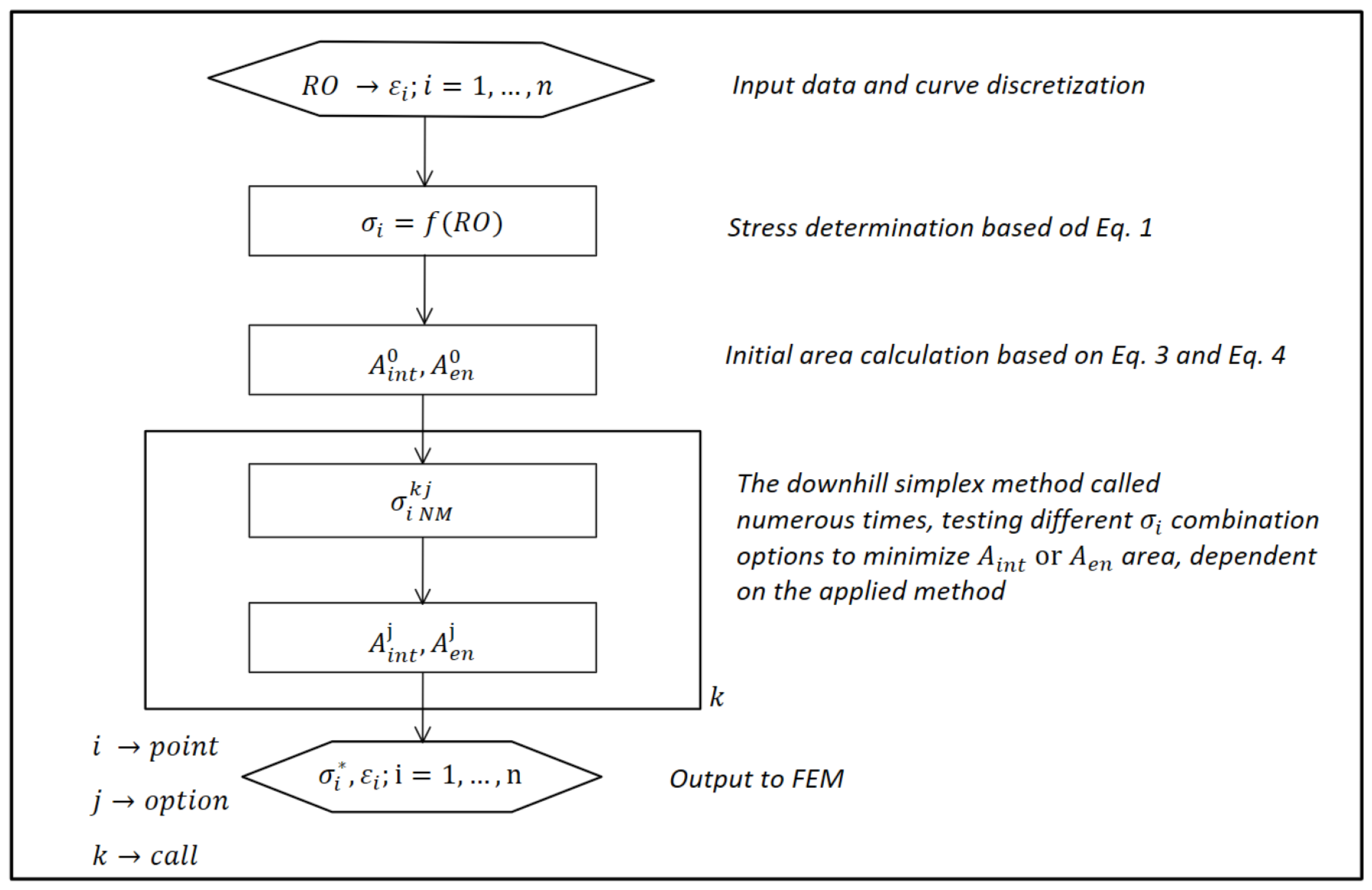The computational algorithm for optimising the stress–strain curve interpolation of a material based on Equation (1) is presented in Figure 3. Initially, the values of ${\epsilon }_i$ are chosen and the values of ${\sigma }_i$ are calculated using Equation (1). To integrate the area between the input and the interpolated curve without knowing the analytical expression, Equation (2) can be reformulated as

$$A_{\mathit{int}}=\sum _{i=1}^n\left|\left|{\int }_0^{{\epsilon }_i}{\sigma }_d\left(\epsilon \right)d\epsilon -{\int }_0^{{\epsilon }_{i-1}}{\sigma }_d\left(\epsilon \right)d\epsilon \right|-\left|{\int }_0^{{\epsilon }_i}{\sigma }_m\left(\epsilon \right)d\epsilon -{\int }_0^{{\epsilon }_{i-1}}{\sigma }_m\left(\epsilon \right)d\epsilon \right|\right|.$$

(4)

However, this approach requires a finely discretised strain axis for the given curves. If the discretisation is too coarse, a significant integration error will occur where the actual and the modelled curves intersect. For Equation (3), no reformulation is needed due its simplicity. Using Equations (3) and (4), the initial areas $A_{en}^0$ and $A_{int}^0$ are calculated. This is followed by an iterative process of finding the optimal ${\sigma }_i^{*}$ values for the minimisation of either A_int or A_en using the Nelder–Mead algorithm. The rate of function minimisation is dependent on the number of times the function is called using the Nelder–Mead algorithm. Since values of $A_{int}^j$ or $A_{en}^j$ converge to a constant, it makes sense to terminate the iterative process early enough to avoid unnecessarily prolonging the computational time, but not too early to ensure the results are not inadequate.

To achieve acceptable computation times during the optimisation, only the stress values of the yield planes are modified, while the strains are left at their initially computed values. The initial points on the curve, where both stress and strain values are zero, and the points of the last yield plane remain unchanged during the optimisation routine. To obtain an interpolated curve that is a close representation of the input curve, initial guess values are used from points on the input curve, as shown in Figure 4a. This also accelerates the downhill simplex method in finding the optimal stress values for minimising the value of A_int since the minimal value can only be achieved by one combination of stress values. A graphical representation of the methods in comparison to the conventional linear interpolation is shown in Figure 4 for a bilinear curve example where the stress value of $q_1$ yield planes is optimised. As depicted in Figure 4, even the position of a single stress–strain point to divide the elastic from the plastic region offers several options. The interspace minimisation method with area A_int (Figure 4c) obviously ensures the most suitable position of the stress–strain point as compared to the conventional interpolation (Figure 4a) and the energy dissipation method with area A_en (Figure 4b).

3. Results and Discussion

These methods were applied to available experimental results for an EN 1.4512 steel [6] and PA12 [28] polymer. Although only two shapes of the stress–strain curves were used to apply the interpolation methods, they encompass all the crucial features, e.g., nonlinear elastoplasticity, monotonically increasing stress–strain relation with decreasing strain rate in case of EN 1.4512 steel, monotonically increasing stress–strain relation with increasing strain rate in case of PA12 and an inflection point in case of PA12. The software code for both material responses is included as the Supplementary Material to this paper. The reader can apply the code to other materials containing features not included in the examples. As the result of either of the optimisation methods, a set of stress–strain points was observed that can be used to represent the cyclic curve with multilinear characteristics. The obtained stress–strain points gained by either of the optimisation methods were then evaluated by the sizes of A_int or A_en and the computational time as a function of the number of yield planes, ranging from a bilinear curve to 33 yield planes. The elastoplastic response of the EN 1.4512 steel was simulated with the RO parameters obtained at three experimental temperatures of 20 °C, 300 °C and 650 °C, as shown in

Table 1. Material properties of ferritic stainless steel EN 1.4512 at test temperatures of 20 °C, 300 °C and 650 °C [6].

T [°C]	E [MPa]	K′ [MPa]	n′ [-]	Rm [MPa]	σp [MPa]
20	200,000	603.42	0.1211	407	140
300	180,000	508.16	0.1103	360	120
650	150,000	183.13	0.0336	165	90

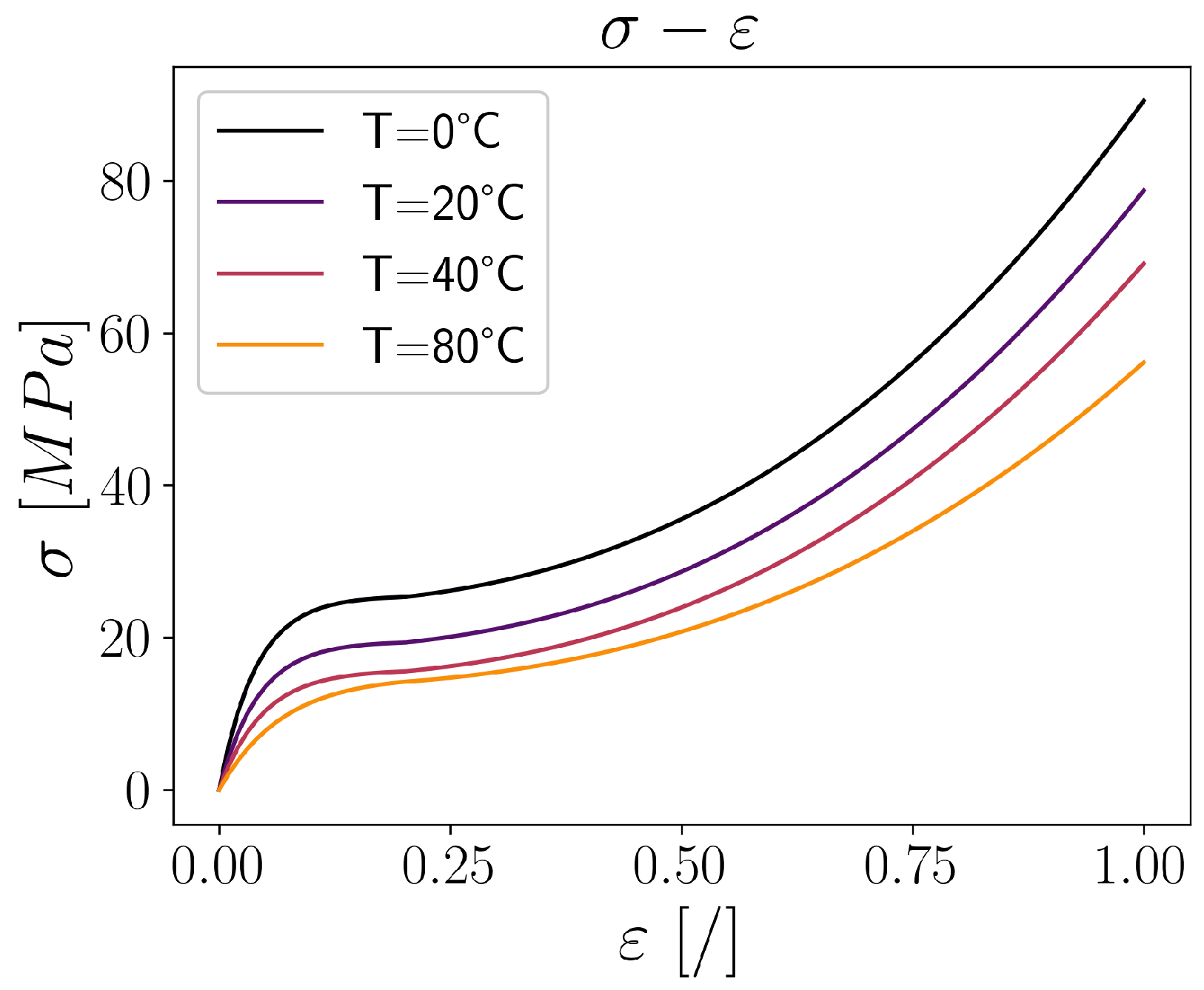
[6]. For the polymer material PA12, the curves at four different temperatures of 0 °C, 20 °C, 40 °C and 80 °C [28] were directly imported in terms of their stress–strain points. They are given in Figure 5. For a statistical evaluation of the conventional interpolation and the energy dissipation method, a total of 500 temperatures were considered, whereas for the interspace minimisation method, which proved to be slower, a total of 20 temperatures were used.

Increasing the number of yield planes swiftly decreases both A_int and A_en areas. Graphical representation of the resulting stress–strain curves therefore provides little information regarding the differences between the methods. Hence, looking at the values of areas A_int and A_en with respect to the number of yield planes provides clearer insight into the method comparison. 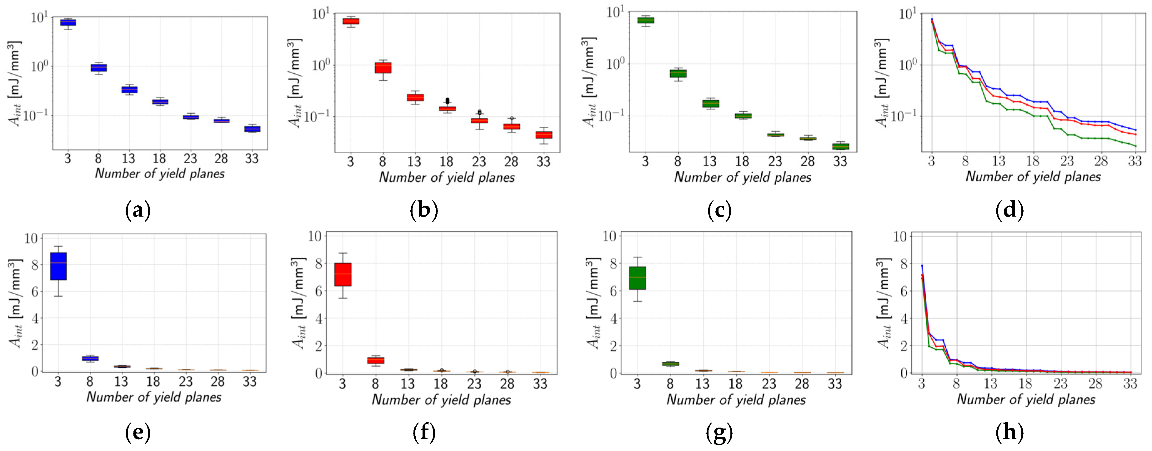Box-plots were chosen to present the statistical evaluation of the A_int and A_en values. 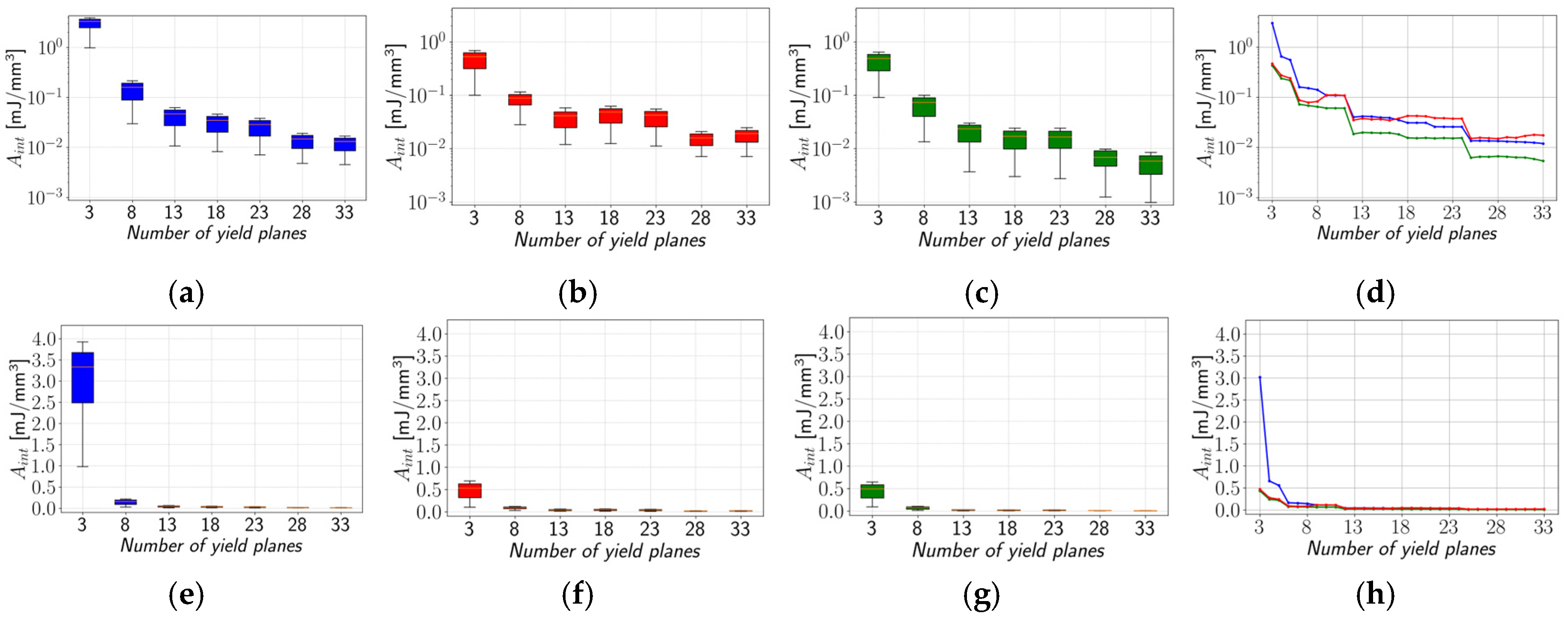In Figure 6a–c, the A_int values are depicted for EN 1.4512 steel using a logarithmic scale for the three sets of stress–strain results gained using the interpolation methods. The comparison between the mean A_int values is then shown in Figure 6d. The A_int values are also presented in Figure 6e–h using a linear scale. As expected, the lowest values of A_int are obtained with the interspace minimisation method regardless of the number of yield planes. The difference between the conventional interpolation and the interspace minimisation method is most significant at smaller numbers of yield planes, especially when using bilinear interpolation. Meanwhile, the energy dissipation method seems more unstable considering the A_int value at 18 yield planes is higher than at 13 yield planes and that its value at 33 yield planes is higher than that of the conventional interpolation. Interestingly, since the energy dissipation minimisation method has an infinite number of possible solutions, the A_int value will not always decrease as the number of yield planes increases. A similar trend as for EN 1.4512 steel can be observed in Figure 7a–d for the PA12 material using a logarithmic scale and in Figure 7e–h, using a linear scale.

A similar comparison for the A_en values is carried out next. However, the observed A_en values of the energy dissipation method cannot be discussed since the primary goal of this method is to eliminate A_en. The results of the remaining two methods are depicted in Figure 8a,b. Furthermore, since the A_en values can deviate from positive to negative values, a logarithmic scale cannot be applied. As shown in Figure 1a–c, conventional interpolation of a stress–strain curve is acquired with the Ramberg–Osgood equation results in the interpolation curve that is bounded above by the original stress–strain curve. Therefore, the A_en value of the conventional interpolation method is equal to its A_int value. Considering that the integrated area under the stress–strain curve represents the energy required to fracture the material, a positive A_en value means that the required energy for the interpolated curve is smaller than for the actual curve. As shown in Figure 8b, this is not the case for the interspace minimisation method. Overall, the absolute value of A_en is smaller than that of the conventional interpolation, but negative A_en values mean that material toughness is overestimated. Figure 8c indicates that the interspace minimisation method offers an overall improvement over conventional interpolation, especially at a low number of yield planes. In contrast to EN 1.4512 steel, the conventional interpolation applied to the polymer material PA12 can result in negative A_en values (Figure 9a). Therefore, the application of the interspace minimisation method reduces the absolute size of the A_en value (Figure 9b,c), which also reduces the overestimation of material toughness.

The computational time is examined in Figure 10a,b. The calculations were performed using an Intel Core i7-7820HQ 4-Core processor and 32 GB of RAM. The interspace minimisation method was tested using a smaller number of temperatures; therefore, the computational running time was adapted for the number of temperatures used for the testing of the remaining two methods. Since conventional interpolation does not involve an iterative process, its running time is independent of the number of yield planes, making it the fastest of the three methods. The computational time of the energy dissipation method increases with the amount of yield planes applied due to the need for a higher number of downhill simplex algorithm iterations to achieve convergence of the A_en value. The same principle applies to the interspace minimisation method, with its longer iteration time than that of the energy dissipation method due to only one possible outcome of stress combinations. As is clearly seen in Figure 10a,b, the computational time of the interspace minimisation method significantly differs from the other two methods. If the iteration limit was not set beforehand, it would differ even more. Interestingly, there is no obvious difference between computational times when applying the methods to either EN 1.4512 steel or PA12.

In Figure 11a,b, the values of A_en and A_int, each for their respective method as observed during the optimisation runtime, are depicted as functions of the number of downhill simplex algorithm calls for the case of 33 yield planes at a temperature of 20 °C. Both methods converge smoothly to their minimal values. In Figure 11c,d, these results are presented for the PA12 curve at 0 °C and 33 yield planes. In Figure 11c, it can be observed that the starting value of A_en is higher than that of the EN 1.4512 steel in Figure 11a. Nonetheless, the energy dissipation method still converges with a low number of iterations. This is due to the fact that a very small value of A_en can be achieved by an infinite number of stress value combinations at given yield planes. This also means that the energy dissipation method is prone to returning stress–strain curves that are not monotonically increasing. Therefore, providing the downhill simplex method with good initial guesses of stress values is critical for achieving sensible results. On the contrary, the interspace minimisation method can converge to only one possible result. Therefore, providing the interspace minimisation method with bad initial guesses of stress values or overly coarse curve discretisation, as shown in Figure 11d, where the starting value of A_int is much higher than that in Figure 11b due to a more complex curve shape, results in a higher number of required function calls, but the output of the method will not necessarily change. This makes the interspace minimisation method much more stable and reliable than the energy dissipation method.

4. Conclusions

The interspace minimisation method, as presented in this study, offers an optimisation of stress–strain curve interpolation for a more accurate description of material parameters. The cyclic stress–strain curves for EN 1.4512 steel and a PA12 polymer were discretised using the interspace minimisation method and then compared to the conventional interpolation method and energy dissipation method. The interspace minimisation method proved much more stable and reliable than the energy dissipation method regardless of the number of discretisation points. However, the computational time of the interspace minimisation method was significantly higher than the computational time of the other two methods, which follows from the unambiguity of stress–strain point positions. On the contrary, the conventional interpolation and the energy dissipation method were computationally more effective but the positions of their stress–strain points were not as restrained as in the case of the interspace minimisation method. The presented algorithm is complementary to the multiaxial Prandtl operator approach for the temperature-dependent elastoplastic problem given by Nagode et al. [16,29] and will be applied to mechanical components, such as in [18], as part of future work. However, the determination of optimal stress–strain positions is independent of the mechanical component under scrutiny and is therefore carried out prior to the FEA following the same steps as in this study.