Loess Collapsibility Prediction and Influencing Factor Analysis Using Multiple Machine Learning Algorithms in Xi’an Region

Abstract

Collapsibility is a fundamental geotechnical property of loess that critically affects its engineering behavior. In this study, a comprehensive dataset comprising 9041 experimental records on the physical properties and collapsibility of loess from the Xi’an region was compiled. Six parameters were selected as model inputs: sampling depth (H), water content (w), plastic limit (w_P), plasticity index (I_P), compression coefficient (a_1–2), and compression modulus (E_s). Based on these inputs, prediction models for the loess collapsibility coefficient (δ_s) were developed using Gaussian Process Regression (GPR), Gradient Boosting Machine (GBM), Support Vector Regression (SVR), Radial Basis Function Neural Network (RBFNN), Classification and Regression Tree (CART), and Feature Tokenizer Transformer (FT-Transformer). Among these, GPR demonstrated the best predictive performance, achieving the lowest error (RMSE = 9.88 × 10⁻³) and the highest accuracy (R² = 0.844). Additionally, the coverage proportion of the 95% confidence interval of the GPR predictions reached 0.949. SHapley Additive exPlanations (SHAP) analysis for GPR further revealed that the compression coefficient exerted the greatest influence on δ_s (0.0149), followed by compression modulus (0.0080), water content (0.0068), plasticity index (0.0061), sampling depth (0.0061), and plastic limit (0.0052). The GPR-based prediction model offers significantly higher predictive accuracy than empirical models. The developed models provide a robust technical framework for the rapid estimation of loess collapsibility in the Xi’an region.

1. Introduction

Loess is extensively distributed worldwide, covering nearly 10% of the Earth’s land surface. It is predominantly found in arid and semi-arid regions [1,2]. In northwestern China, collapsible loess represents the most widespread soil type [3]. Insufficient understanding of its collapsibility in engineering practice can result in severe geotechnical hazards, including slope instability, ground subsidence, and tunnel failure. These hazards pose substantial risks to public safety and infrastructure [4,5,6,7]. Consequently, accurate evaluation of the collapsibility of loess and its influencing factors is of critical importance for engineering construction in loess regions.

To accurately predict the collapsibility of loess, researchers have developed a variety of assessment approaches based on in situ [8,9] and laboratory [10,11,12] testing. For example, Shao [13] proposed an in situ sand well water seepage saturated loess test and conducted four tests at different depths at a loess site along the Baoji–Lanzhou high-speed railway. The results demonstrated that this method effectively reflects differences in collapsibility and provides valuable reference basis for evaluating collapsibility and foundation treatment in loess tunnel engineering. Nie [14] introduced a resistivity-based method for characterizing the collapsibility of compacted loess. The experiment developed a model to predict collapsibility coefficient using resistivity, water content, and dry density, enabling rapid and reliable evaluation of loess collapsibility. Despite their reliability, these conventional methods typically demand substantial manpower, materials, and time for procedures such as sampling, packaging, and transportation. In addition, their applicability is often constrained by testing conditions, construction schedules, and project costs, which ultimately hinders their efficacy in addressing the practical demands of engineering projects.

In addition, a number of studies have examined the correlations between loess collapsibility and its physical properties using statistical approaches [15,16]. Zheng et al. [6] combined spatial modeling with experimental data and identified water content, dry density, pressure, and elevation as key controlling factors. Their work not only delineated high-risk zones of loess collapsibility in the Lvliang region but also pioneered the integration of spatial correlation into collapsibility studies, offering new perspectives for disaster prevention. Wang et al. [17] analyzed compression curves from six loess sites and established correlation models linking compressibility to initial structural features and physical indices. Their results showed close agreement with in situ tests, enabling reliable classification of collapsibility types and grades, and providing a practical evaluation tool in cases where field testing is infeasible. However, regression-based approaches are generally restricted to linear or simple nonlinear relationships and thus perform poorly when capturing the complex nonlinear interactions among soil variables. In recent years, machine learning has advanced rapidly, offering powerful alternatives to address these limitations and to improve the prediction accuracy of the collapsibility coefficient. For instance, Mu et al. [18] and Zhu et al. [19] used physical indices as input variables and applied multivariate expression programming (MEP) to predict loess collapsibility, achieving high accuracy and demonstrating the potential of data-driven methods in geotechnical investigations. Similarly, Fan et al. [20] further emphasized the role of pore size and particle morphology as dominant factors and developed a Genetic Algorithm Support Vector Machine (GA-SVM) model with enhanced applicability and predictive accuracy for loess collapsibility. Despite these advances, notable limitations remain. First, most existing studies are based on relatively small datasets, which increases the risk of overfitting and reduces the generalization ability of machine learning models. Second, the range of methods explored has been narrow, with prior studies applying only a limited subset of algorithms. As a result, the relative performance of different machine learning approaches in predicting loess collapsibility has not been comprehensively evaluated.

In Xi’an, a substantial volume of geotechnical and collapsibility test data has been accumulated through engineering construction projects. Leveraging this resource, the present study aims to enable rapid and accurate prediction of the loess collapsibility coefficient (δ_s). The multicollinearity analysis is first employed to eliminate collinearity among the physical property indices. Multiple machine learning models are then developed and systematically compared to evaluate their predictive capabilities. The use of a large dataset helps to overcome the limitations of small-sample studies and significantly enhances the generalization capacity of the models. The best-performing model is further benchmarked against conventional empirical approaches to highlight its practical advantages. In addition, SHapley Additive exPlanations (SHAP) analysis is conducted to quantitatively assess the relative contribution of each physical parameter, thereby elucidating the key factors controlling loess collapsibility. Finally, a comparison based on practical engineering applications confirmed the potential of the model for real-world implementation. The main contribution of this study lies in the use of a large-scale dataset comprising 9041 samples of loess physical and collapsibility properties. Subsequently, six machine learning models, including Gaussian Process Regression (GPR), Gradient Boosting Machine (GBM), Support Vector Regression (SVR), Radial Basis Function Neural Network (RBFNN), Classification and Regression Tree (CART), and Feature Tokenizer Transformer (FT-Transformer), were applied to predict the collapsibility of loess, and their predictive performances were systematically compared. The comparison includes both the baseline models and conventional empirical models. Furthermore, SHAP analysis was employed to interpret the machine learning models and elucidate the influence of each physical property on the predicted collapsibility. Finally, the models with excellent performance are applied to actual engineering cases to evaluate their practical prediction accuracy. The novelty of this study lies in the first application of the FT-Transformer to the prediction of loess collapsibility, combined with SHAP analysis to achieve model interpretability. The findings of this study provide technical support for predicting the loess collapsibility coefficient in the Xi’an region.

2. Study Area

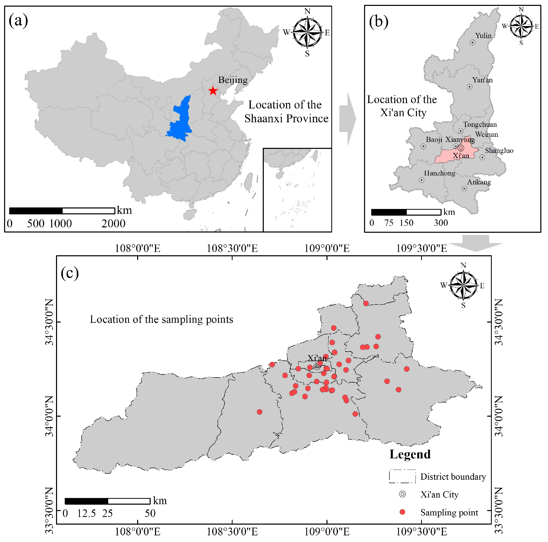
Xi’an, the capital city of Shaanxi Province, is situated between 107°40′ E–109°49′ E and 33°42′ N–34°45′ N, covering a total area of approximately 1.01 × 10⁴ km². The study area lies in the central Guanzhong Plain within the Weihe River Basin and is characterized by a warm temperate, semi-humid continental monsoon climate, with distinct seasons, moderate temperatures, and evenly distributed annual precipitation. The mean annual rainfall ranges from 530 to 700 mm, of which nearly 45% occurs between July and September.

Geologically, the region is underlain by thick deposits of collapsible loess, which exhibit significant settlement upon wetting, a critical geotechnical property that strongly influences engineering construction. In this study, extensive data on loess collapsibility were compiled to analyze its regional characteristics. The locations of the sampling sites are shown in Figure 1c. The dataset consists of laboratory test data collected between 2019 and 2024.

3. Materials and Methods

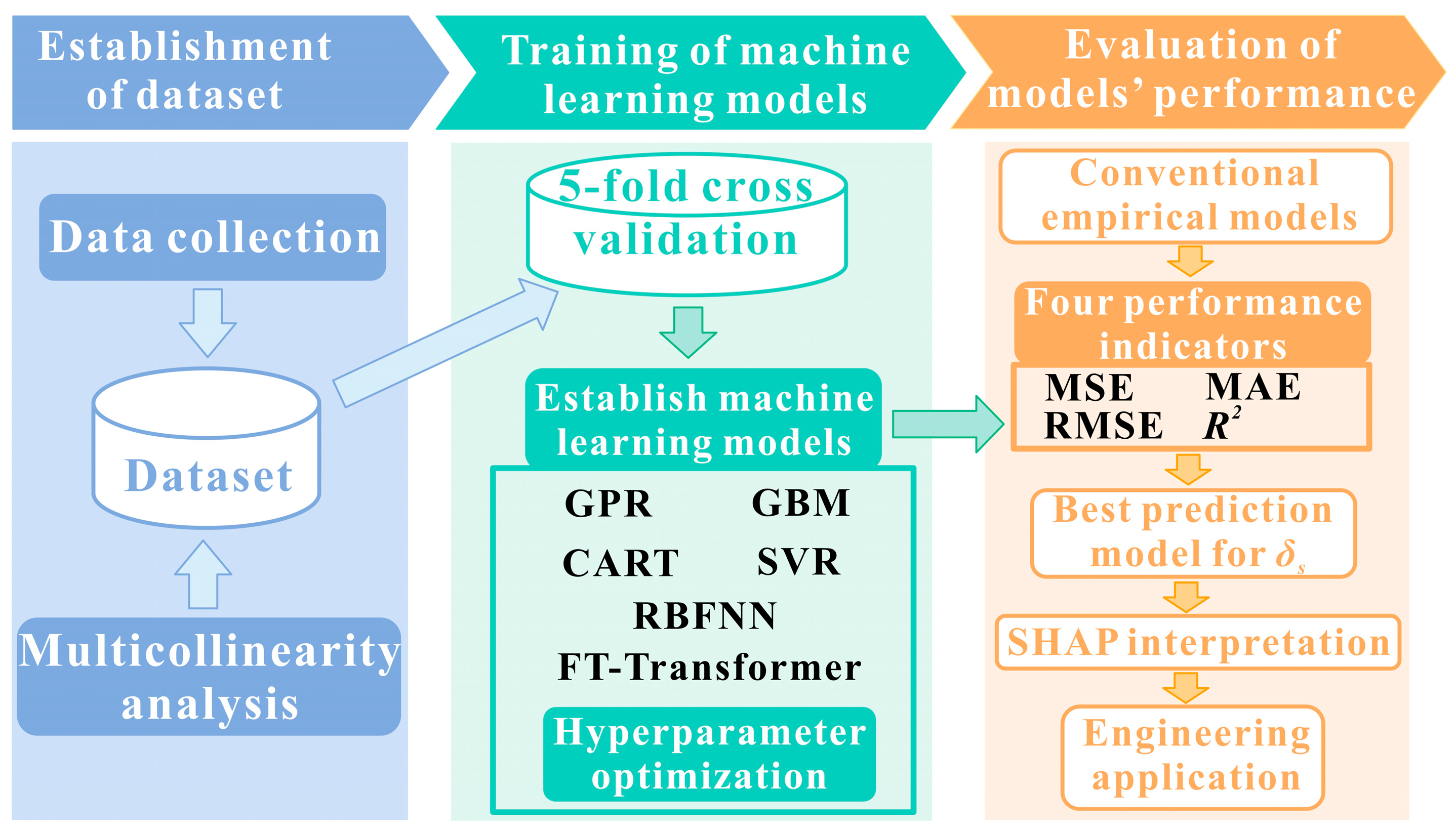
The overall workflow of this study is illustrated in Figure 2. Xi’an was selected as the research area, and the dataset was established using physical indices of loess together with its collapsibility coefficient (δ_s). Statistical and Multicollinearity analysis were first conducted to examine the relationships among the variables. On this basis, six machine learning models, including Gaussian Process Regression (GPR), Gradient Boosting Machine (GBM), Classification and Regression Tree (CART), Support Vector Regression (SVR), Radial Basis Function Neural Network (RBFNN), and Feature Tokenizer Transformer (FT-Transformer), were developed to predict δ_s. The hyperparameters of each model were optimized using a grid search algorithm. Five-fold cross validation was simultaneously employed to comprehensively evaluate model performance and determine the optimal machine learning regression model. The best-performing model was then benchmarked against conventional empirical approaches for validation. SHapley Additive exPlanations (SHAP) analysis was applied to quantify the relative contribution of each physical index, thereby revealing the dominant factors governing loess collapsibility. Finally, the trained models were applied to a real-world engineering case, and the results demonstrated their practical applicability.

3.1. Machine Learning Regression Algorithms

(1)

Gaussian Process Regression (GPR)

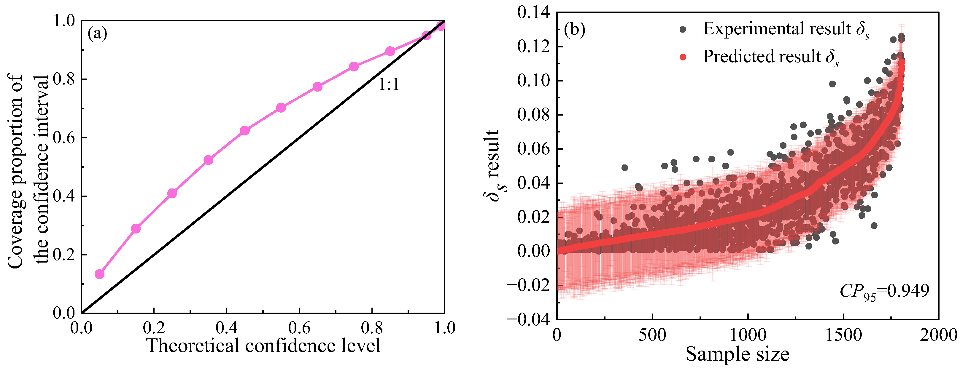
Gaussian Process Regression (GPR) is a non-parametric Bayesian approach to regression that employs a Gaussian Process (GP) prior [21]. The method was systematically elaborated by Rasmussen [22,23]. GPR is particularly advantageous in its ability to model complex functional relationships and to automatically capture latent correlations within data. Additionally, GPR provides the standard deviation of its predictions, which can be used to calculate prediction confidence intervals, which is also important in geotechnical engineering applications. Typically, the coverage proportion of the 95% confidence interval (CP₉₅) [21] is used to represent the proportion of δ_s experimental values falling within the predicted interval. The 95% confidence interval is calculated as (Equation (1)):

$$C{P}_{95}={\delta }_s^{pred}\pm 1.96{\sigma }_{{\delta }_s^{pred}}$$

(1)

where ${\delta }_s^{pred}$ denotes the predicted δ_s value and ${\sigma }_{{\delta }_s^{pred}}$ denotes the standard deviation of the prediction.

(2)

Support Vector Regression (SVR)

Support Vector Regression (SVR), originally proposed by Vapnik [24], is based on the ε-insensitive loss function, which disregards prediction errors that fall within an ε margin. By applying kernel functions, SVR maps input data from the original feature space into a higher dimensional space, thereby enabling effective treatment of nonlinear regression problems [25,26] (Equation (2)):

$$y(x)=W^T\times h(x)+b$$

(2)

where W denotes the weight matrix; h(x) represents the nonlinear mapping to a high dimensional feature space; b is the bias term. Since the SVR model does not impose any constraints on the predicted values of δ_s, negative predictions may occur. To address this issue, the input data were transformed before prediction, and the output was subsequently restored to ensure that the predicted δ_s values remain greater than zero. Specifically, δ_s was transformed prior to modeling as shown in Equation (3):

$${\delta }_s^{\prime }=\log ({\delta }_s+\zeta )$$

(3)

$${\delta }_s^{pred}=\exp ({\delta }_s^{\prime })-\zeta$$

(4)

After prediction, the inverse transformation was performed according to Equation (4) to ensure that the output values remain greater than zero. In this process, δ_s denotes the original collapsibility coefficient, δ_s′ represents the transformed value of δ_s, and ζ is a small constant close to zero. This prevents the model from producing negative δ_s values.

(3)

Radial Basis Function Neural Network (RBFNN)

The Radial Basis Function Neural Network (RBFNN) [27] is a single-hidden-layer feedforward neural network. Unlike conventional neural networks, RBFNN employs a radial basis function as the activation function in the hidden layer, while the output layer is expressed as a linear combination of the hidden layer neurons [28,29]. To ensure non-negative model outputs, the Rectified Linear Unit (ReLU) activation function is applied to the output layer. The ReLU function has a range of $[0,+\mathrm{\infty })$, which prevents negative δ_s values (Equation (5)).

$$\phi (x)=\mathrm{ReLU}({\displaystyle \sum _{i=1}^q{M}_i\rho (x,c_i))}$$

(5)

where q denotes the number of hidden layer neurons; c_i and M_i represent the center and weight matrix of the i-th neuron, respectively; ρ(x, c_i) is the radial basis function, and ReLU denotes the Rectified Linear Unit activation function.

(4)

Gradient Boosting Machine (GBM)

The Gradient Boosting Machine (GBM) [30] is a variant of the boosting algorithm in ensemble learning. Its core principle is to construct a series of weak learners in a sequential manner, with each learner trained to reduce the residual errors of its predecessor, thereby producing a strong predictive model [31]. GBM is well known for its high accuracy, flexibility, and robustness [32,33].

(5)

Classification and Regression Tree (CART)

The Classification and Regression Tree (CART) algorithm [34] partitions the data space into multiple regions, each corresponding to a specific output [35]. At each branching step, the algorithm determines the optimal split by minimizing the squared error, which is achieved by evaluating all possible features and threshold values. The prediction for each leaf node is then given by the mean value of the samples contained in that node. Consequently, the output space is divided into M regions, denoted as R₁, …, R_M (Equation (6)).

$$f(x)={\displaystyle \sum _{m=1}^M{c}_{m}I(x\in R_m)}$$

(6)

where c_m denotes the output value of the m-th partitioned region, and I (x ∈ R_m) is the indicator function.

(6)

Feature Tokenizer Transformer (FT-Transformer)

The Feature Tokenizer Transformer (FT-Transformer) is a transformer-based model specifically designed for tabular data. By incorporating embeddings and multi-head attention mechanisms, it can capture complex relationships among variables. The model was originally developed by Gorishniy et al. [36] as an enhancement of the standard transformer architecture [37], which has been widely applied across various fields [38,39,40]. The input vector x is transformed into an embedding T. For numerical features, the embedding is computed as follows (Equation (7)):

$$T=b+x\cdot W$$

(7)

where b denotes the bias term and W denotes the weight matrix. The embedding T is then fed into the Transformer layers to produce the final output.

3.2. Data Collection

In this study, experimental data were compiled from loess engineering projects in the Xi’an region, comprising a total of 9041 records of loess physical properties and collapsibility. Ten physical indices were considered: sampling depth (H), water content (w), natural density (ρ), dry density (ρ_d), initial void ratio (e₀), liquid limit (w_L), plastic limit (w_P), plasticity index (I_P), compression coefficient (a_1–2), and compression modulus (E_s). The loess collapsibility coefficient (δ_s) was used as the target variable. Among them, a_1–2 and E_s were measured under a stress range of 0.1 MPa to 0.2 MPa.

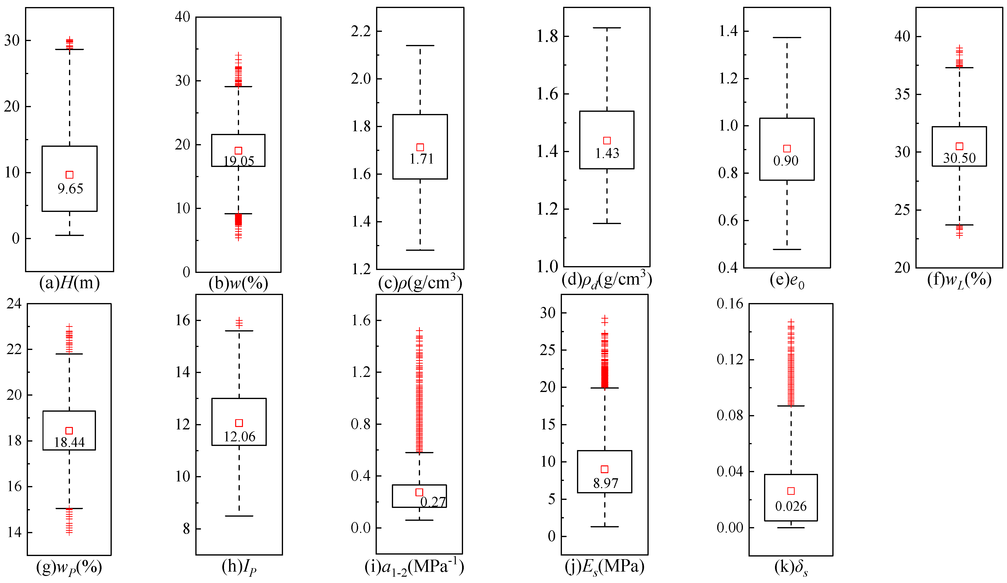
Figure 3 presents boxplots of the ten influencing factors together with δ_s, where red squares denote the mean values. It can be observed that the compression coefficient (a_1–2) exhibits a relatively large number of outliers (Figure 3i), while sampling depth (H), natural density (ρ), dry density (ρ_d), initial void ratio (e₀), liquid limit (w_L), plastic limit (w_P), and plasticity index (I_P) show more concentrated distributions.

4. Results

4.1. Multicollinearity Analysis of the Data

The loess collapsibility coefficient (δ_s) is governed by multiple physical properties. Multicollinearity analysis is an important data preprocessing step in the prediction of collapsibility in loess. When a strong correlation exists between physical property indicators, it indicates that the corresponding indicator may not be suitable as an input variable for the model [41]. Multicollinearity is commonly assessed using the pair of statistical metrics: tolerance (TOL) and variance inflation factor (VIF), which are reciprocals of each other. Generally, a TOL value greater than 0.1 (i.e., VIF < 10) indicates that the indicator is not strongly correlated with other variables. The results of the multicollinearity analysis are presented in

Table 1. Results of the multicollinearity analysis.

Physical Properties (Units)	TOL	VIF
H (m)	0.82	1.21
w (%)	0.66	1.51
ρ (g/cm3)	1.39 × 10−3	719.23
ρd (g/cm3)	1.87 × 10−3	533.77
e0	8.84 × 10−3	113.07
wL (%)	4.83 × 10−2	20.69
wP (%)	0.22	4.50
IP	0.19	5.29
a1–2 (MPa−1)	0.32	3.09
Es (MPa)	0.36	2.76

.

Based on the results of the multicollinearity analysis, the TOL values natural density (ρ), dry density (ρ_d), initial void ratio (e₀), and liquid limit (w_L) are all below 0.1, with corresponding VIF values exceeding 10, indicating severe multicollinearity between these indicators and the others. Therefore, they should be excluded as input variables in machine learning models. In contrast, sampling depth (H), water content (w), plastic limit (w_P), plasticity index (I_P), compression coefficient (a_1–2), and compression modulus (E_s) exhibit TOL values greater than 0.1 and VIF values less than 10, indicating relative independence among these variables; thus, they are suitable to serve as input features for machine learning models. As shown in Figure 3i,j, numerous outliers are observed in the compression coefficient and compression modulus data. However, these outliers are genuine measurements. Blindly removing them could significantly degrade the model’s predictive performance when encountering extreme samples. Therefore, these data points were retained and considered during model development.

4.2. Comparison of the Predictive Performance of Six Models

All machine learning algorithms in this study were implemented in Python (Version 3.8). The SVR, GPR, GBM, and CART models were developed using functions from the scikit-learn library (Version 0.24.2). The RBFNN model was implemented using a combination of PyTorch (Version 1.7.0) and scikit-learn, while the FT-Transformer was built with the rtdl (Version 0.0.13) and PyTorch libraries. The data were standardized before model training. For model training, five-fold cross validation was employed to evaluate the performance of the models [29,42,43]. Hyperparameters for all six models were optimized using a grid search algorithm, and predictive performance was assessed using four evaluation metrics. During this process, five-fold cross validation was employed to evaluate the performance of the optimization. The hyperparameter optimization results are presented in

Table 2. Optimization results of model hyperparameters.

Model	Hyperparameter	Optimal Value
GPR	Kernel function	Rational quadratic kernel function
	Length scale	0.74
	Scale mixture	0.175
SVR	Kernel function	RBF
	Constant C	0.11
	ε-insensitive parameter	0.015
	RBF kernel parameter γ	0.192
RBFNN	Hidden layer node	70
	RBF parameter γ	1.5
	Learning rate	0.1
GBM	Number of weak learners	900
	Maximum tree depth	7
	Learning rate	0.015
CART	Maximum tree depth	6
	Minimum number of samples required to split a node	13
	Minimum number of samples per leaf	6
FT-Transformer	Token dimension	64
	Number of transformer layer	4
	Dropout rate	0.016
	Learning rate	2 × 10−4

.

To evaluate the accuracy of predicting the loess collapsibility coefficient (δ_s), four metrics were applied to the validation sets of the six models: Root Mean Squared Error (RMSE), Mean Squared Error (MSE), Mean Absolute Error (MAE), and the coefficient of determination (R²).

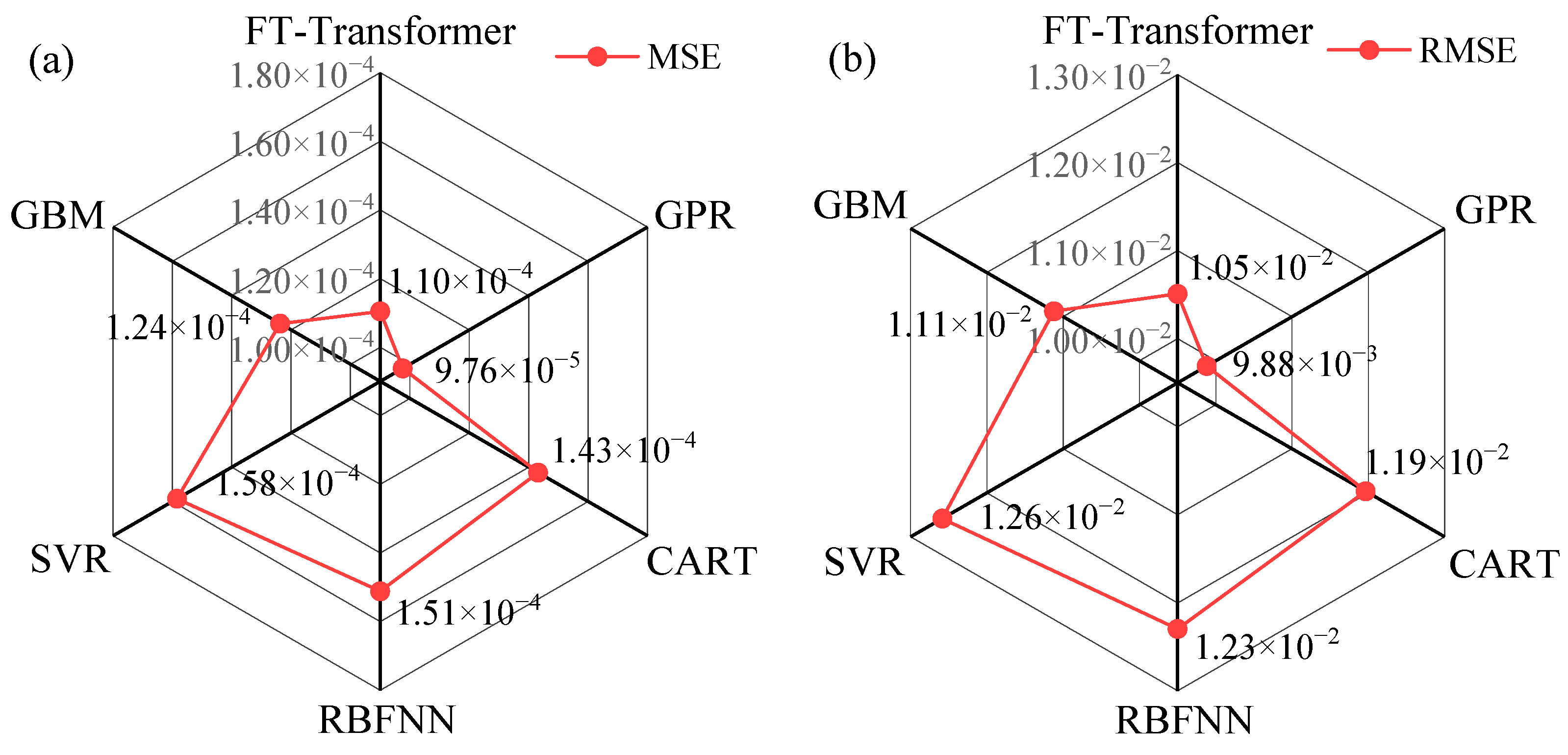
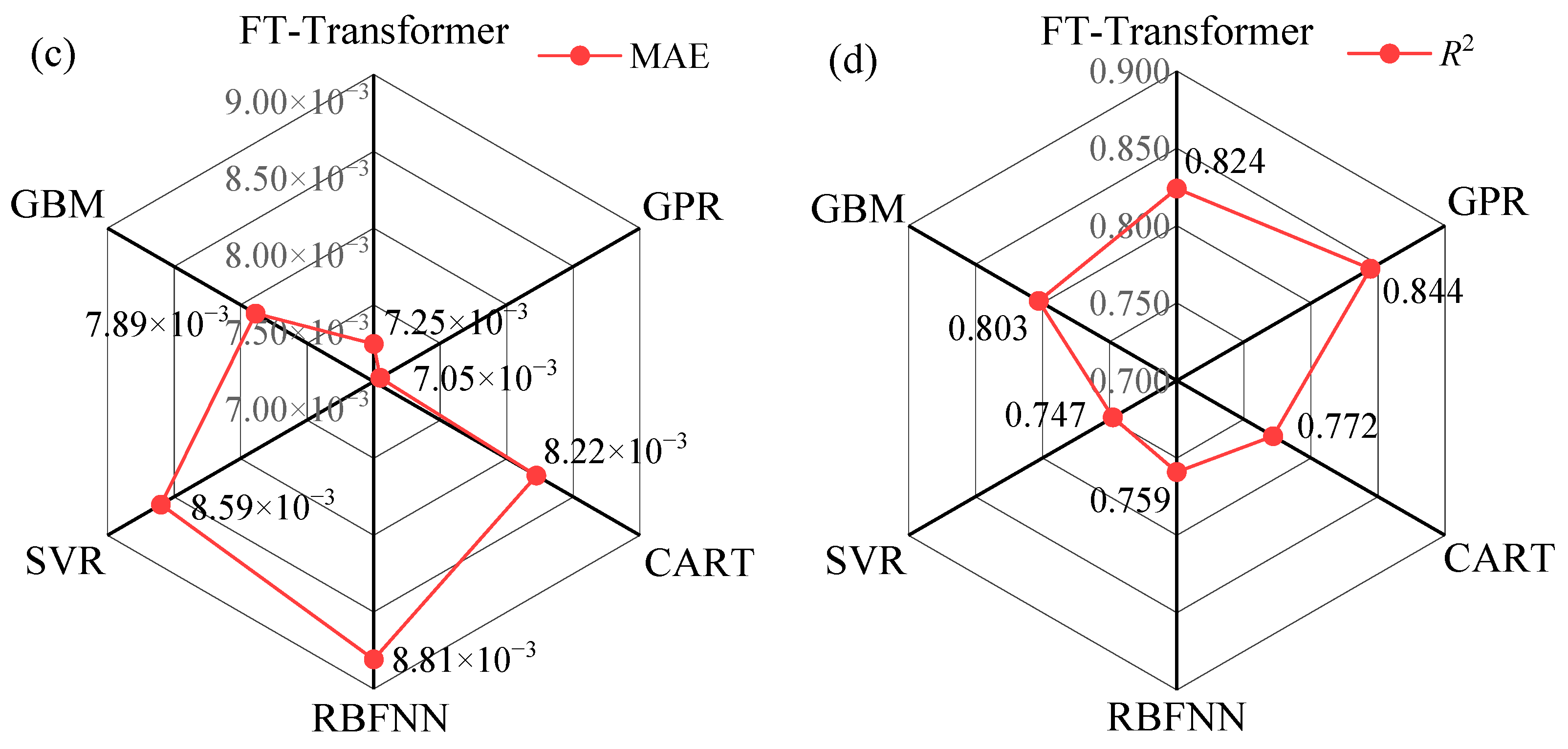
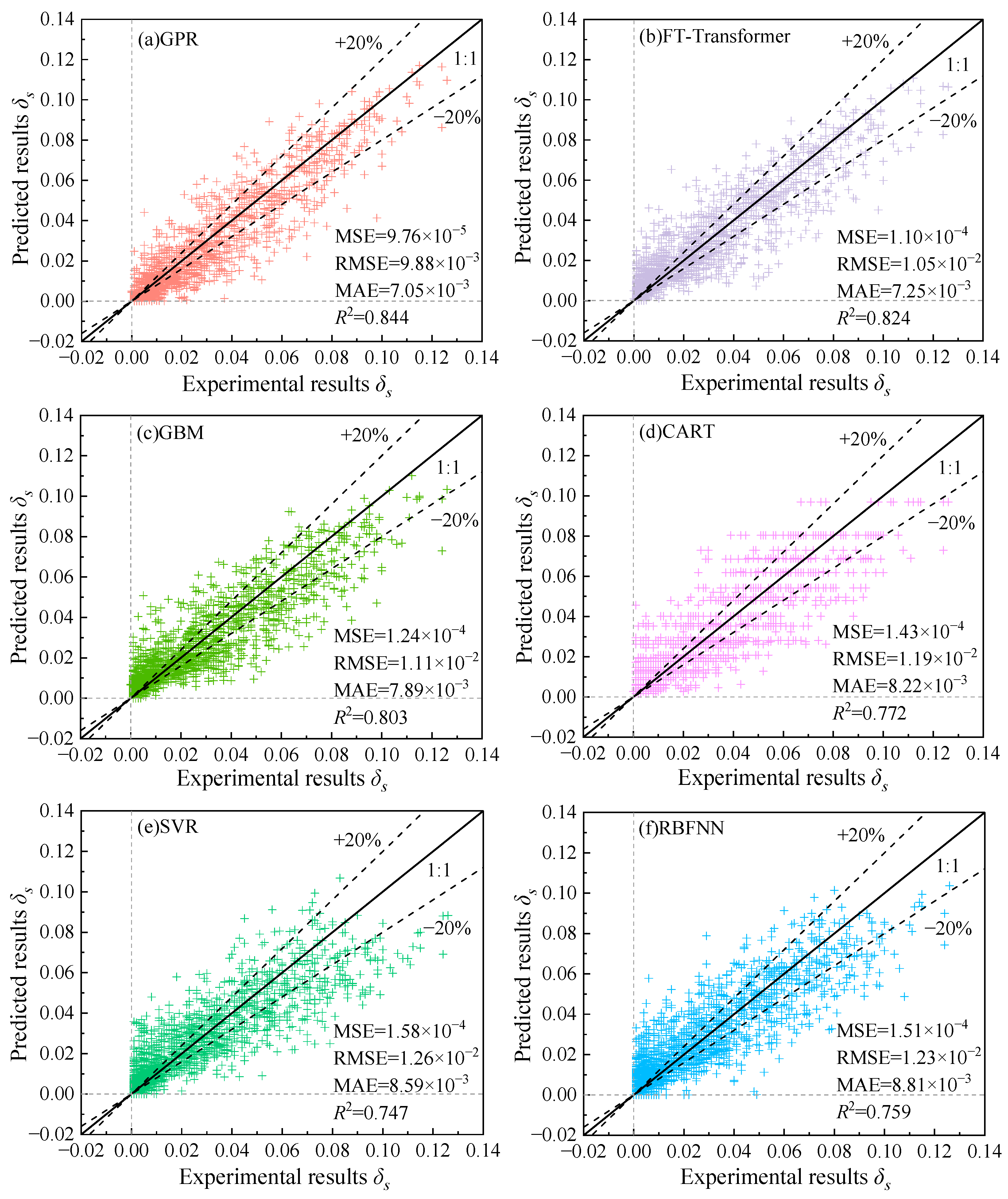
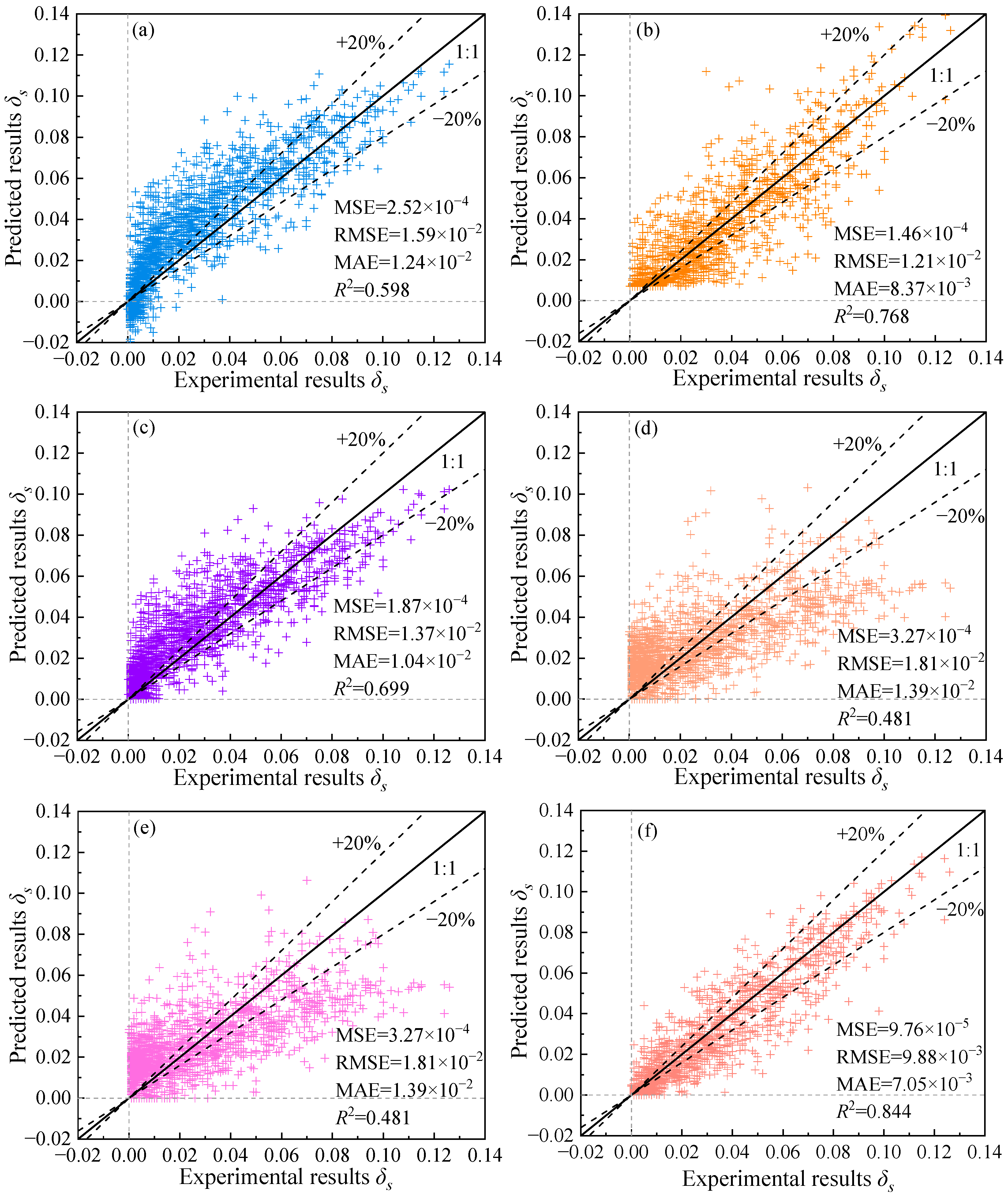
Figure 4 and

Table 3. Performance evaluation for machine learning models.

Model	MSE (Mean ± Std)	RMSE (Mean ± Std)	MAE (Mean ± Std)	R2 (Mean ± Std)
SVR	1.58 × 10−4 ± 8.2 × 10−6	1.26 × 10−2 ± 3.3 × 10−4	8.59 × 10−3 ± 1.4 × 10−4	0.747 ± 0.005
RBFNN	1.51 × 10−4 ± 5.5 × 10−6	1.23 × 10−2 ± 2.2 × 10−4	8.81 × 10−3 ± 1.6 × 10−4	0.759 ± 0.008
CART	1.43 × 10−4 ± 6.9 × 10−6	1.19 × 10−2 ± 2.9 × 10−4	8.22 × 10−3 ± 1.5 × 10−4	0.772 ± 0.008
GBM	1.24 × 10−4 ± 7.5 × 10−6	1.11 × 10−2 ± 3.3 × 10−4	7.89 × 10−3 ± 1.5 × 10−4	0.803 ± 0.017
FTT	1.10 × 10−4 ± 2.1 × 10−5	1.05 × 10−2 ± 9.3 × 10−4	7.25 × 10−3 ± 7.0 × 10−4	0.824 ± 0.037
GPR	9.76 × 10−5 ± 1.3 × 10−5	9.88 × 10−3 ± 6.0 × 10−4	7.05 × 10−3 ± 4.4 × 10−4	0.844 ± 0.029

present the statistical results of the four metrics for all machine learning models. Among them, the GPR and FT-Transformer achieved lower error-based values (MSE, RMSE, MAE) and higher R², indicating superior predictive capability. To further demonstrate model performance, Figure 5 compares experimental δ_s with predicted values, where the experimental δ_s is plotted on the x-axis and the predicted δ_s on the y-axis. The scatter plots show that the predictions of the GPR model cluster more closely around the 1:1 line, with most points falling within a ±20% error band. Moreover, the GPR model achieved lower error metrics and a higher R² compared with the FT-Transformer. Meanwhile, the standard deviations of the GPR model’s performance metrics were within acceptable ranges. Therefore, the GPR model is considered to provide the most accurate and reliable predictions of δ_s among the six evaluated models.

In general, conventional SVR and RBFNN models do not impose constraints on the output range, which may result in negative predictions of the collapsibility coefficient δ_s. However, δ_s is inherently a positive quantity. In this study, both the SVR and RBFNN models were modified to ensure non-negative outputs. The corresponding results are presented in Figure 5e,f. As shown, neither model produced negative predictions after the modification. Nevertheless, their error metrics (MSE, RMSE, MAE) were higher, and the coefficient of determination (R²) was lower than those of the other models. These results indicate that the modified SVR and RBFNN models exhibited inferior predictive performance for δ_s compared with the other four methods. Considering the results presented in Figure 4 and Figure 5, GPR demonstrates the best predictive performance for δ_s, followed by FT-Transformer, GBM, CART, RBFNN, and SVR, in descending order.

The GPR model outputs the standard deviation of the predicted results, which can be used to estimate the confidence interval of the model predictions. In geotechnical engineering applications, these confidence intervals provide valuable reference information for assessing prediction reliability.

Table 4. Summary table of GPR model calibration results.

Theoretical Confidence Level	Coverage Proportion of the Corresponding Confidence Interval
0.05	0.133
0.15	0.289
0.25	0.410
0.35	0.524
0.45	0.624
0.55	0.703
0.65	0.774
0.75	0.843
0.85	0.895
0.95	0.949
0.99	0.982

presents the theoretical confidence levels and their corresponding confidence interval coverage proportions. Figure 6a visualizes these data as a calibration curve. When the theoretical confidence level is below 0.85, the corresponding coverage proportions are slightly higher than the theoretical values. At the 0.95 and 0.99 confidence levels, CP₉₅ = 0.949 and CP₉₉ = 0.982, indicating that the model achieves near-ideal calibration performance. As shown in Figure 6b, the red transparent band represents the confidence interval of each predicted value. The calculated CP₉₅ value is 0.949, indicating high credibility and demonstrating that the GPR model provides accurate predictions of the collapsibility coefficient (δ_s).

4.3. Quantitative Analysis of Input Variables on the Loess Collapsibility Coefficient

To further investigate the influence of each physical property on the loess collapsibility coefficient (δ_s), SHapley Additive exPlanations (SHAP) values [44] were employed. SHAP provides a framework for interpreting machine learning predictions, thereby improving model transparency and explainability. The GPR and FT-Transformer models that exhibited superior predictive performance were selected for feature importance analysis, as illustrated in Figure 7 and Figure 8. For the GPR model, the importance of the input features, in descending order, is as follows: compression coefficient (0.0149), compression modulus (0.0080), water content (0.0068), plasticity index (0.0061), sampling depth (0.0061), and plastic limit (0.0052). For the FT-Transformer model, the order of feature importance is compression coefficient (0.0223), compression modulus (0.0161), sampling depth (0.0066), water content (0.0056), plasticity index (0.0026), and plastic limit (0.0021).

4.4. Comparison with Conventional Methods

Previous studies on predicting the collapsibility of loess have primarily relied on polynomial regression equations. To validate the rationality and accuracy of the present study, regression equations proposed by earlier scholars [45,46,47] were selected, in which the collapsibility coefficient (δ_s) was expressed as a function of loess physical properties. In addition, based on the dataset used in this study, multiple linear regression (MLR) and partial least squares regression (PLS) models were developed to predict the loess collapsibility coefficient. These models were used as baseline references for comparison. The fitted equations are presented in

Table 5. Regression equations fitted using MLR and PLS.

Model	Regression Equation
MLR	$\begin{array}{l}{\delta }_s=0.0466-0.000922H-0.002544w+0.004935w_P\\ -0.005913I_P+0.05712a_{1-2}+0.000099E_s\end{array}$
PLS	$\begin{array}{l}{\delta }_s=0.0545-0.000837H-0.00284w+0.00327w_P\\ -0.003519I_P+0.057432a_{1-2}-0.000049E_s\end{array}$

.

Table 6. Performance comparison between GPR and regression equations.

Model	MSE (Mean ± Std)	RMSE (Mean ± Std)	MAE (Mean ± Std)	R2 (Mean ± Std)
Gao [45]	2.52 × 10−4 ± 9.9 × 10−6	1.59 × 10−2 ± 3.1 × 10−4	1.24 × 10−2 ± 1.9 × 10−4	0.598 ± 0.031
Guo [46]	1.46 × 10−4 ± 1.1 × 10−5	1.21 × 10−2 ± 4.5 × 10−4	8.37 × 10−3 ± 2.1 × 10−4	0.768 ± 0.023
Li [47]	1.87 × 10−4 ± 9.4 × 10−6	1.37 × 10−2 ± 3.3 × 10−4	1.04 × 10−2 ± 2.1 × 10−4	0.699 ± 0.026
MLR	3.27 × 10−4 ± 1.3 × 10−5	1.81 × 10−2 ± 3.6 × 10−4	1.39 × 10−2 ± 2.7 × 10−4	0.481 ± 0.023
PLS	3.27 × 10−4 ± 1.5 × 10−5	1.81 × 10−2 ± 4.1 × 10−4	1.39 × 10−2 ± 3.2 × 10−4	0.481 ± 0.024
GPR	9.76 × 10−5 ± 1.3 × 10−5	9.88 × 10−3 ± 6.0 × 10−4	7.05 × 10−3 ± 4.4 × 10−4	0.844 ± 0.029

summarizes the statistical indicators and standard deviations of previously proposed models, the regression equations fitted in this study, and the GPR model. All models were evaluated using five-fold cross validation. The evaluation metrics predicted by each regression equation were compared with those of the GPR model using paired t-tests, and the results are presented in

Table 7. The p-values from the paired t-test between the polynomial regression model and the GPR model.

Model	p (MSE)	p (RMSE)	p (MAE)	p (R2)
Gao [45]	3.58 × 10−5	4.21 × 10−5	3.13 × 10−5	2.37 × 10−5
Guo [46]	4.83 × 10−3	3.81 × 10−3	1.06 × 10−2	3.67 × 10−3
Li [47]	1.67 × 10−4	1.98 × 10−4	2.09 × 10−4	9.48 × 10−5
MLR	2.02 × 10−5	2.12 × 10−5	1.83 × 10−5	5.53 × 10−6
PLS	2.58 × 10−5	2.52 × 10−5	1.32 × 10−6	1.91 × 10−6

. Both p-values are less than 0.05, indicating that the differences are statistically significant. These results demonstrate that the GPR model exhibits superior performance in predicting the loess collapsibility coefficient (δ_s).

Figure 9 compares scatter plots of predicted versus experimental δ_s values obtained using polynomial regression equations with those predicted by the GPR model developed in this study. Figure 9a,b show the collapsibility regression equations established for the loess in the Xi’an area, while Figure 9c present the equations developed for other regions within the Loess Plateau. Figure 9d,e present the results of the polynomial regression equations fitted using MLR and PLS, respectively. From Figure 9a, it can be observed that 192 of the predicted δ_s values are negative. In contrast, application of the GPR method to the same validation samples produced no negative δ_s values. Furthermore, the error metrics (MSE, RMSE, MAE) for GPR were significantly lower than those of the five polynomial regression models, while the coefficient of determination (R²) was higher. For the polynomial regressions with lower R² values (Figure 9d,e), the scatter plots are more dispersed, with most points deviating markedly from the 1:1 line. Although Figure 9a–c display sample points closer to the 1:1 line, Figure 9a still produces a considerable number of negative δ_s predictions.

4.5. Practical Engineering Applications of the Model

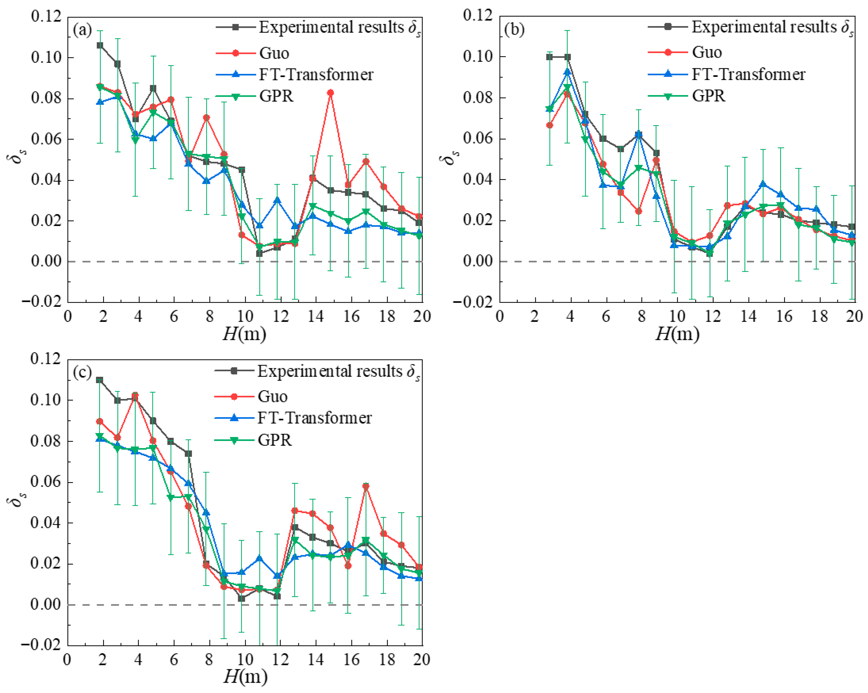
To evaluate the practical applicability of the loess collapsibility prediction models, three borehole datasets from a construction site in the Xi’an area were selected to further evaluate the engineering applicability of the proposed models. When the sampling depth is less than 12 m, the soil is classified as Q₃ loess, while depths greater than 12 m correspond to Q₂ loess. The laboratory compression tests were conducted in accordance with the specifications outlined in the relevant standard [48]. The Gaussian Process Regression (GPR) and FT-Transformer models, which demonstrated superior predictive performance, were compared with Guo’s [46] empirical model. The results are presented in

Table 8. Performance evaluation of the model’s application in practical engineering.

Model	MSE (Mean ± Std)	RMSE (Mean ± Std)	MAE (Mean ± Std)	R2 (Mean ± Std)
Guo [46]	2.79 × 10−4 ± 7.7 × 10−5	1.66 × 10−2 ± 2.3 × 10−3	1.20 × 10−2 ± 2.8 × 10−3	0.699 ± 0.052
FTT	1.87 × 10−4 ± 4.6 × 10−5	1.36 × 10−2 ± 1.7 × 10−3	1.11 × 10−2 ± 2.3 × 10−3	0.793 ± 0.065
GPR	1.35 × 10−4 ± 3.2 × 10−5	1.15 × 10−2 ± 1.3 × 10−3	8.85 × 10−3 ± 7.5 × 10−4	0.854 ± 0.013

and Figure 10.

As shown in Table 8, the GPR model achieved the lowest error metrics (MSE, RMSE, and MAE) and the highest coefficient of determination (R²), indicating superior predictive accuracy. From Figure 10, it can be observed that both the GPR and FT-Transformer models exhibit smaller deviations from the measured collapsibility coefficient (δ_s) than Guo’s empirical model. Moreover, the 95% confidence intervals of the GPR predictions consistently encompassed the experimental δ_s values, demonstrating the model’s high reliability.

5. Discussion

5.1. Model Construction and Performance

In engineering projects in the Xi’an region, the collapsibility of loess must be carefully considered, as inaccurate assessment can result in severe geological hazards [49]. In this study, multicollinearity analysis was conducted to identify suitable physical indices for machine learning modeling [50,51]. The results indicated that the variance inflation factors (VIFs) of natural density (ρ), dry density (ρ_d), initial void ratio (e₀) and liquid limit (w_L) were relatively high. From a geotechnical perspective, liquid limit (w_L), as a key indicator reflecting soil plasticity and fine particle content, exhibits intrinsic functional relationships with plastic limit (w_P) and plasticity index (I_P). Similarly, the significant multicollinearity observed among natural density (ρ), dry density (ρ_d), and initial void ratio (e₀) is physically reasonable. Specifically, dry density (ρ_d) can be derived from natural density (ρ) and water content (w), while initial void ratio (e₀) is closely related to dry density (ρ_d) and can be calculated from dry density and particle specific gravity. Consequently, these three variables essentially describe the same aspects of soil pore structure, resulting in strong redundancy and elevated VIF values. From a modeling standpoint, strongly correlated variables should be avoided to reduce redundant information and improve model stability.

To validate the rationality of the multicollinearity analysis, this study employed Principal Component Analysis (PCA) for comparison. PCA extracted three principal components, denoted as Y₁, Y₂, and Y₃. The results are summarized in

Table 9. Principal component analysis results.

Principal Component	Principal Component Equation
Y1	$\begin{array}{l}{Y}_1=0.148H+0.208w+0.434\rho +0.404{\rho }_d-0.401e_0\\ +0.329w_L+0.295w_P+0.341I_P-0.264a_{1-2}+0.194E_s\end{array}$
Y2	$\begin{array}{l}{Y}_2=-0.215H+0.259w-0.175\rho -0.285{\rho }_d+0.301e_0\\ +0.436w_L+0.428w_P+0.413I_P-0.292a_{1-2}-0.227E_s\end{array}$
Y3	$\begin{array}{l}{Y}_3=0.103H-0.369w-0.325\rho -0.227{\rho }_d+0.215e_0\\ +0.160w_L+0.230w_P+0.074I_P-0.449a_{1-2}+0.602E_s\end{array}$

, where all soil physical properties were standardized prior to analysis. The cumulative variance contribution of the three principal components reached 0.82. First, the data were subjected to PCA for dimensionality reduction, and GPR and FT-Transformer models were subsequently established. The results are presented in

Table 10. Performance evaluation for FT-Transformer and GPR models.

Model	MSE (Mean ± Std)	RMSE (Mean ± Std)	MAE (Mean ± Std)	R2 (Mean ± Std)
FTT	1.46 × 10−4 ± 3.7 × 10−6	1.20 × 10−2 ± 1.5 × 10−4	7.79 × 10−3 ± 3.8 × 10−5	0.767 ± 0.013
GPR	1.34 × 10−4 ± 3.9 × 10−6	1.15 × 10−2 ± 1.6 × 10−4	7.46 × 10−3 ± 4.8 × 10−4	0.786 ± 0.012

. Comparing Table 10 with Table 3, it is evident that using multicollinearity analysis to select variables achieves better model performance than PCA-based dimensionality reduction. Therefore, this study employed multicollinearity analysis for variable selection.

In studies predicting the loess collapsibility coefficient (δ_s), machine learning approaches should adopt supervised learning methods appropriate for regression tasks. To comprehensively assess predictive performance, this study employed six representative models: GPR, FT-Transformer, GBM, CART, RBFNN, and SVR. These models encompass diverse algorithmic paradigms, with GPR representing a Bayesian non-parametric method, FT-Transformer a deep learning architecture tailored for tabular data, GBM a boosting-based ensemble learning method, CART a decision tree algorithm, RBFNN an artificial neural network, and SVR an extension of support vector machines for regression. By selecting models across these categories, this study enables a systematic comparison of their effectiveness in predicting the loess collapsibility coefficient (δ_s).

Based on the prediction results, GPR, as a non-parametric learning method, achieved the smallest prediction errors and the highest coefficient of determination (R²). Additionally, the coverage proportion of the 95% confidence interval (CP₉₅) reached 0.949. The results indicate that non-parametric approaches are more suitable for predicting the loess collapsibility coefficient (δ_s). From the calibration results, the actual coverage rates of the GPR model at various confidence levels are very close to the theoretical values, indicating that its uncertainty estimation is reliable. At lower confidence levels, the actual coverage is slightly higher than the theoretical expectation, suggesting that the model is somewhat conservative and produces slightly wider confidence intervals. This conservatism is beneficial in engineering applications, as it helps prevent the model from underestimating the risk of collapse, thereby improving the safety and reliability of geotechnical designs. This reliable uncertainty quantification can directly enhance safety in engineering design. Since CP₉₅ = 0.949, the upper bound of the 95% predictive confidence interval can be used as a safety reference in design. This approach is equivalent to adding a safety margin to the GPR model predictions, thereby incorporating model uncertainty into the engineering design’s safety factor. Consequently, it enables more robust risk management and control. The FT-Transformer, although a more complex deep learning architecture, achieved slightly lower accuracy than GPR. GBM, which integrates multiple base learners and iteratively reduces residual error, provided stable results, while CART produced predictions with a more regular distribution (Figure 5d). However, this regularity reflects the limitations of its binary tree structure, which restricts generalization ability. For SVR and RBFNN, unmodified models can inevitably produce negative predictions. By constraining the output of the SVR model (Equations (3) and (4)) and applying the ReLU activation function to the output layer of RBFNN (Equation (5)), the occurrence of negative predictions was effectively suppressed. However, the overall predictive performance of these models remained suboptimal, resulting in inferior performance compared with the other models.

As the only deep learning model in this study, the FT-Transformer was further evaluated for its rationality by comparing it with a Multilayer Perceptron (MLP). The main hyperparameters of the MLP included the hidden layer size, activation function, dropout rate, and learning rate. Through grid search optimization, these hyperparameters were determined to be (32, 16), ReLU, 0.1, and 0.01, respectively. The hyperparameter tuning was also conducted using five-fold cross-validation. The prediction results of the MLP are summarized in

Table 11. Performance evaluation for MLP model.

Model	MSE (Mean ± Std)	RMSE (Mean ± Std)	MAE (Mean ± Std)	R2 (Mean ± Std)
MLP	1.62 × 10−4 ± 1.7 × 10−5	1.27 × 10−2 ± 6.9 × 10−4	9.36 × 10−3 ± 4.6 × 10−5	0.740 ± 0.035

.

By comparing Table 11 with Table 3, it can be observed that the FT-Transformer achieves lower error metrics (MSE, RMSE, MAE) and a higher R² value, indicating that its predictive performance for the loess collapsibility coefficient (δ_s) surpasses that of the MLP. The collapsibility of loess is influenced by multiple interacting variables. The MLP relies on fixed hidden-layer connections for feature aggregation, which limits its ability to capture dynamic feature interactions effectively. In contrast, the FT-Transformer employs a self-attention mechanism that adaptively models complex and nonlinear relationships among features. This mechanism allows the model to automatically identify and emphasize the features that contribute most to δ_s, thereby enhancing both its representational capacity and generalization performance.

The results of this study were compared with the previous researchers and with regression equations fitted using the same dataset. The results demonstrate that the GPR model achieved the highest predictive performance. A simple linear combination of soil physical indices often produced large deviations from experimental values, as the relationships between loess indices and the collapsibility coefficient (δ_s) are inherently nonlinear. Consequently, the models shown in Figure 9d,e performed poorly. In contrast, Figure 9f shows that the predictions of GPR aligned more closely with the experimental values, while the results of the five polynomial regression models were markedly more scattered. This advantage arises because GPR, as a non-parametric regression method based on Gaussian process priors, effectively captures nonlinear dependencies between loess properties and δ_s through kernel functions. Conventional polynomial regression, however, relies on a predefined functional form and adjusts only weights and bias terms, limiting its ability to represent complex nonlinear relationships. Paired t-test results revealed significant differences between the GPR model and the polynomial regression models, indicating that GPR possesses superior capability in capturing nonlinear relationships and quantifying predictive uncertainty, both of which are critical in geotechnical engineering applications. Based on the above analysis, the GPR model demonstrates a distinct advantage in evaluating the loess collapsibility coefficient (δ_s), providing an effective and reliable approach with high predictive accuracy. Moreover, the comparison between polynomial regression and machine learning models underscores the potential of artificial intelligence techniques for investigating and characterizing the collapsibility of loess in the Xi’an region.

Based on Figure 7 and Figure 8, the compression coefficient (a_1–2) and compression modulus (E_s) have the most significant influence on the collapsibility coefficient (δ_s). Among them, the compression coefficient exerts a strongly positive effect. The compression modulus (E_s), sampling depth (H), water content (w), plastic limit (w_P) and plasticity index (I_P) negatively influence the model predictions. The compression coefficient (a_1–2) and compression modulus (E_s) reflect the loess’s resistance to compressive deformation. During the collapsibility deformation stage, cementing materials dissolve and soil particles rearrange, causing structural collapse and increased compressibility. This manifests macroscopically as an increase in the collapsibility coefficient and compression coefficient, and a decrease in the compression modulus. As sampling depth increases, soil density generally rises. Additionally, deeper soils are typically older, resulting in lower collapsibility. Generally, higher water content reduces effective stress due to increased pore water pressure, making soils with higher initial moisture softer and more deformable during the initial loading stage of laboratory tests. Consequently, higher water content is associated with reduced soil porosity, indicating a negative correlation with the collapsibility coefficient. The plasticity index represents the range of soil plasticity. Higher liquid limit and plasticity index indicate a high clay content, small pores, and a dense structure, making the soil less prone to collapsibility upon wetting. Thus, both show a negative correlation with the collapsibility coefficient. By integrating the physical interpretation of each loess property with microstructural analysis, the SHAP results can be well explained.

For both the GPR and FT-Transformer models, the compression coefficient (a_1–2) and compression modulus (E_s) are the most important variables, whereas the influence of the plastic limit (w_P) is relatively minor. This consistency in SHAP-based feature importance indicates that the compression coefficient and compression modulus should be given particular attention when predicting the loess collapsibility coefficient (δ_s). The importance of water content (w), sampling depth (H), and plasticity index (I_P) shows slight differences between the two models. These differences arise from the inherent structural distinctions: GPR is a non-parametric prediction method, whereas FT-Transformer is a deep learning approach. Given their fundamentally different modeling principles, variations in how they capture data patterns are to be expected.

To evaluate the practical applicability of the proposed models, borehole data from a geotechnical project in Xi’an were used to compare the performance of the GPR and FT-Transformer models. In addition, a representative empirical model with relatively good performance was incorporated for comparative analysis. The results show that both GPR and FT-Transformer perform well in practical applications, outperforming the empirical model. As shown in Figure 10, the collapsibility coefficient of loess generally decreases with increasing sampling depth. A sharp decline occurs around a depth of 12 m, after which the coefficient rises again beyond this depth. With increasing depth, the overburden stress on the soil also increases. At approximately 12 m, the self-weight consolidation of the soil reaches a relatively saturated state, leading to a significant reduction in void ratio. The soil structure becomes denser, and the interparticle bonding strengthens, resulting in a lower collapsibility coefficient. However, when the depth exceeds 12 m, the collapsibility coefficient increases again. This phenomenon can be attributed to the higher content of soluble carbonates in older loess layers, which makes the soil more prone to collapse upon wetting. The trend is consistently captured by all three methods. In terms of predictive performance, both GPR and FT-Transformer achieve better results than the empirical model, with GPR achieving slightly superior metrics overall. In engineering practice, the collapsibility coefficient is a critical parameter for calculating foundation settlement and classifying foundation treatment levels. Prediction bias in machine learning models may lead to inaccurate estimations of soil collapsibility, thereby affecting foundation design decisions. Therefore, the uncertainty of model predictions should be fully considered and transformed into a quantifiable safety margin during foundation design. For example, the design collapsibility coefficient can be determined based on the upper confidence limit derived from the predicted mean and variance. This strategy ensures structural safety while balancing construction cost and risk control, enabling a data-driven and reliable foundation design approach. The GPR model provides a stable 95% confidence interval, which encompasses all experimental δ_s values. This demonstrates the higher reliability and robustness of the GPR model. Consequently, the GPR model offers valuable reference potential for practical geotechnical investigations in loess regions.

5.2. Limitations and Future Prospects

Although the dataset in this study is extensive, it is geographically limited to the Xi’an region. The loess in this area was mainly deposited during the Quaternary and exhibits good particle-size sorting. However, due to variations in formation history, climatic conditions, and parent material across different regions, loess can differ in microstructure, mineral composition, and cementation degree. These regional differences may alter the quantitative relationships between soil physical properties and the collapsibility coefficient, thereby limiting the model’s transferability.

To address this limitation, regional characteristics should be considered during model development, and the model must be recalibrated before applying it to loess from other areas. Future work could expand the dataset to multiple loess regions and employ regional clustering to capture spatial heterogeneity, or adopt transfer learning strategies to fine-tune the model using local datasets. Specifically, future work will first involve collecting sample data from multiple representative regions where collapsible loess is distributed, to capture the variations in microstructure and mineral composition among different areas. Second, a transfer learning framework will be established to leverage the knowledge learned from the Xi’an loess dataset. Through parameter fine-tuning or feature adaptation, the model can be effectively transferred to new regional datasets. In cases where data from other regions are limited, adversarial feature alignment techniques can be explored to enhance feature adaptation and maintain model robustness across different loess conditions. Such approaches would enable the model to adapt to the specific properties of loess in different regions while retaining features learned from the Xi’an dataset. Additionally, incorporating supplementary input variables, such as mineral composition and microstructural indicators, could enhance the model’s physical interpretability and cross-regional robustness. Accounting for these factors would allow the collapsibility prediction model to be applied across regions with diverse geological and climatic conditions.

6. Conclusions

In this study, a comprehensive dataset of 9041 records of loess physical properties and collapsibility was compiled from the Xi’an region. Multicollinearity analysis was used to eliminate correlations among the physical parameters. Six machine learning algorithms, Gaussian Process Regression (GPR), Gradient Boosting Machine (GBM), Support Vector Regression (SVR), Radial Basis Function Neural Network (RBFNN), Classification and Regression Tree (CART), and Feature Tokenizer Transformer (FT-Transformer), were applied to predict the loess collapsibility coefficient (δ_s). The predictive performance of the algorithms was evaluated using four error-based and accuracy-based metrics, and SHAP analysis was performed on the superior performing model to interpret feature importance. Finally, the optimal machine learning model was benchmarked against conventional polynomial regression approaches. The main conclusions are as follows:

(1)

Through multicollinearity analysis, highly collinear physical indices were eliminated. In this study, six loess physical parameters were selected as input variables for the machine learning models, including sampling depth (H), water content (w), plastic limit (w_P), plasticity index (I_P), compression coefficient (a_1–2) and compression modulus (E_s).

(2)

Among the six machine learning models tested, GPR achieved the highest predictive accuracy (R² = 0.844), with the coverage proportion of the 95% confidence interval (CP₉₅) of 0.949. followed by FT-Transformer (R² = 0.824), GBM (R² = 0.803), CART (R² = 0.772), and RBFNN (R² = 0.759). SVR performed the poorest, with an R² of only 0.747.

(3)

When polynomial regression equations were used to estimate δ_s, the R² values were 0.598, 0.768, 0.699, 0.481, and 0.481, respectively. Compared with these polynomial regression models, the GPR model showed substantially closer agreement with experimental values, demonstrating its superior capability for accurately predicting δ_s.

(4)

In the prediction of loess collapsibility in the Xi’an region, the compression coefficient (a_1–2) and compression modulus (E_s) were identified as the most influential variables in both the GPR and FT-Transformer models, whereas the plastic limit (w_P) had a comparatively lower impact. Therefore, greater attention should be given to the compression coefficient (a_1–2) and compression modulus (E_s) when predicting loess collapsibility.

(5)

In practical engineering applications, the GPR model demonstrated superior performance in predicting the loess collapsibility coefficient compared with both the conventional empirical model and the FT-Transformer. Moreover, the GPR predictions exhibited high confidence levels, indicating that the model provides valuable reference potential for real-world geotechnical investigations.

References

1. Li, P.; Vanapalli, S.; Li, T. Review of collapse triggering mechanism of collapsible soils due to wetting. J. Rock Mech. Geotech. Eng. 2016, 8, 256–274. [Google Scholar] [CrossRef]
2. Xie, W.; Li, P.; Zhang, M.; Cheng, T.; Wang, Y. Collapse behavior and microstructural evolution of loess soils from the Loess Plateau of China. J. Mt. Sci. 2018, 15, 1642–1657. [Google Scholar] [CrossRef]
3. Feng, S.; Du, F.; Shi, Z.; Shui, W.; Tan, K. Field study on the reinforcement of collapsible loess using dynamic compaction. Eng. Geol. 2015, 185, 105–115. [Google Scholar] [CrossRef]
4. Derbyshire, E. Geological hazards in loess terrain, with particular reference to the loess regions of China. Earth-Sci. Rev. 2001, 54, 231–260. [Google Scholar] [CrossRef]
5. Duan, Z.; Song, K.; Zhang, N.; Zheng, L.; Yan, X.; Zhang, M. Characteristics and mechanisms of soil structure damage under salt weathering. Soil Tillage Res. 2024, 238, 106030. [Google Scholar] [CrossRef]
6. Zheng, Z.; Li, X.; Wang, L. A longitudinal analysis of collapsibility with predictions over the southeastern Loess Plateau in China. Sci. Rep. 2021, 11, 23824. [Google Scholar] [CrossRef] [PubMed]
7. Jia, J.; Ding, Z.; Gao, C.; Gong, X.; Zhang, C. Space Effect of Loading–Unloading Stress Path Evolution of Roof Strata and Surrounding Rock Control in Deep Mining. Rock Mech. Rock Eng. 2025, 8, 1–23. [Google Scholar] [CrossRef]
8. Lv, Y.; Deng, L.; Fan, W. Loess collapsibility characteristics of railway engineering sites using large-scale trial immersion pit experiments. Bull. Eng. Geol. Environ. 2021, 80, 3271–3291. [Google Scholar] [CrossRef]
9. Xu, Y.; Wang, J.; Gu, T.; Zhang, D.; Ma, W.; Wang, S. Study on the Loess Immersion Test of Metro Line 2 in Xi’an, Shaanxi Province, China. Adv. Civ. Eng. 2021, 2021, 6654391. [Google Scholar] [CrossRef]
10. Nie, Y.; Ni, W.; Tuo, W.; Wang, H.; Yuan, K.; Zhao, Y. Collapsibility deterioration mechanism and evaluation of compacted loess with sodium sulfate under drying–wetting cycles. Nat. Hazards 2022, 115, 971–991. [Google Scholar] [CrossRef]
11. Singhal, S.; Sharma, R.S.; Phanikumar, B.R. A laboratory study of collapse behaviour of remoulded loess under controlled wetting and flooding. Geomech. Geoengin. 2015, 11, 159–163. [Google Scholar] [CrossRef]
12. Jing, Y.; Jia, Z.; Zhang, Z.; Lv, Y.; Wang, L.; Tao, C. Study on the method for determination of the maximum depth of loess collapsible under overburden pressure. Bull. Eng. Geol. Environ. 2019, 79, 1509–1521. [Google Scholar] [CrossRef]
13. Shao, S.; Shao, S.; Li, J.; Zhu, D. Collapsible deformation evaluation of loess under tunnels tested by in situ sand well immersion experiments. Eng. Geol. 2021, 292, 106257. [Google Scholar] [CrossRef]
14. Nie, Y.; Ni, W.; Wang, H.; Yuan, K.; Tuo, W.; Li, X. Evaluation of Collapsibility of Compacted Loess Based on Resistivity Index. Adv. Mater. Sci. Eng. 2021, 2021, 9990012. [Google Scholar] [CrossRef]
15. Li, Z.; Li, X.; Zhu, Y.; Dong, S.; Hu, C.; Fan, J. Mining and analysis of multiple association rules between the Xining loess collapsibility and physical parameters. Sci. Rep. 2021, 11, 816. [Google Scholar] [CrossRef]
16. Yao, Y.; Zhang, Y.; Zhao, Y.; Bai, Y.; Zhang, S.; Cao, C. The evaluation of artificial filling in loess areas by in-situ tests based on statistical analysis. Environ. Earth Sci. 2021, 80, 438. [Google Scholar] [CrossRef]
17. Wang, L.; Shao, S.; She, F. A new method for evaluating loess collapsibility and its application. Eng. Geol. 2020, 264, 105376. [Google Scholar] [CrossRef]
18. Mu, Q.; Song, T.; Lu, Z.; Xiao, T.; Zhang, L.-m. Evaluation of the collapse susceptibility of loess using machine learning. Transp. Geotech. 2024, 48, 101327. [Google Scholar] [CrossRef]
19. Zhu, X.; Shao, S.; Shao, S. Prediction of collapsibility of loess site based on artificial intelligence: Comparison of different algorithms. Environ. Earth Sci. 2024, 83, 101. [Google Scholar] [CrossRef]
20. Fan, P.; Zhang, L.; Shi, C.; Zhang, Y.; Ding, X.; Cheng, H. Collapsible characteristics and prediction model of remodeled loess. Nat. Hazards 2024, 121, 2245–2264. [Google Scholar] [CrossRef]
21. Song, C.; Zhao, T.; Xu, L.; Huang, X. Probabilistic prediction of uniaxial compressive strength for rocks from sparse data using Bayesian Gaussian process regression with Synthetic Minority Oversampling Technique (SMOTE). Comput. Geotech. 2024, 165, 105850. [Google Scholar] [CrossRef]
22. Rasmussen, C.E. Gaussian Processes in Machine Learning. In Advanced Lectures on Machine Learning: ML Summer Schools 2003, Canberra, Australia, February 2–14, 2003, Tübingen, Germany, August 4–16, 2003, Revised Lectures; Bousquet, O., von Luxburg, U., Rätsch, G., Eds.; Springer: Berlin/Heidelberg, Germany, 2004; pp. 63–71. [Google Scholar]
23. Li, K.; Liu, Y.; Kang, Q. Estimating the thermal conductivity of soils using six machine learning algorithms. Int. Commun. Heat Mass Transf. 2022, 136, 106139. [Google Scholar] [CrossRef]
24. Cortes, C.; Vapnik, V. Support-vector networks. Mach. Learn. 1995, 20, 273–297. [Google Scholar] [CrossRef]
25. Chang, C.; Lin, C. LIBSVM: A library for support vector machines. ACM Trans. Intell. Syst. Technol. (TIST) 2011, 2, 27. [Google Scholar] [CrossRef]
26. Zhang, W.; Guo, J.; Li, Z.; Cheng, R.; Ning, C.; Niu, H.; Liu, Z. Prediction of loess collapsibility coefficient using bayesian optimized random forest model. Sci. Rep. 2025, 15, 25281. [Google Scholar] [CrossRef] [PubMed]
27. Moody, J.; Darken, C.J. Fast Learning in Networks of Locally-Tuned Processing Units. Neural Comput. 1989, 1, 281–294. [Google Scholar] [CrossRef]
28. Hu, Y.; You, J.J.; Liu, J.N.K.; He, T. An eigenvector based center selection for fast training scheme of RBFNN. Inf. Sci. 2018, 428, 62–75. [Google Scholar] [CrossRef]
29. Cai, M.; Hocine, O.; Mohammed, A.S.; Chen, X.; Amar, M.N.; Hasanipanah, M. Integrating the LSSVM and RBFNN models with three optimization algorithms to predict the soil liquefaction potential. Eng. Comput. 2021, 38, 3611–3623. [Google Scholar] [CrossRef]
30. Friedman, J.H. Greedy Function Approximation: A Gradient Boosting Machine. Ann. Stat. 2001, 29, 1189–1232. [Google Scholar] [CrossRef]
31. Liang, W.; Luo, S.; Zhao, G.; Wu, H. Predicting Hard Rock Pillar Stability Using GBDT, XGBoost, and LightGBM Algorithms. Mathematics 2020, 8, 765. [Google Scholar] [CrossRef]
32. Zhou, J.; Li, E.; Yang, S.; Wang, M.; Shi, X.; Yao, S.; Mitri, H.S. Slope stability prediction for circular mode failure using gradient boosting machine approach based on an updated database of case histories. Saf. Sci. 2019, 118, 505–518. [Google Scholar] [CrossRef]
33. Zhou, J.; Li, X.; Mitri, H.S. Comparative performance of six supervised learning methods for the development of models of hard rock pillar stability prediction. Nat. Hazards 2015, 79, 291–316. [Google Scholar] [CrossRef]
34. Breiman, L.; Friedman, J.; Olshen, R.A.; Stone, C.J. Classification and Regression Trees, 1st ed.; Chapman and Hall/CRC: New York, NY, USA, 1984; p. 368. [Google Scholar]
35. Zhao, Q.; Yu, S.; Zhao, F.; Tian, L.; Zhao, Z. Comparison of machine learning algorithms for forest parameter estimations and application for forest quality assessments. For. Ecol. Manag. 2019, 434, 224–234. [Google Scholar] [CrossRef]
36. Gorishniy, Y.; Rubachev, I.; Khrulkov, V.; Babenko, A. Revisiting deep learning models for tabular data. Adv. Neural Inf. Process. Syst. 2021, 34, 18932–18943. [Google Scholar]
37. Vaswani, A.; Shazeer, N.; Parmar, N.; Uszkoreit, J.; Jones, L.; Gomez, A.N.; Kaiser, Ł.; Polosukhin, I. Attention is all you need. In Proceedings of the 31st International Conference on Neural Information Processing Systems, Long Beach, CA, USA, 4–9 December 2017. [Google Scholar]
38. Jaffari, Z.H.; Abbas, A.; Kim, C.-M.; Shin, J.; Kwak, J.; Son, C.; Lee, Y.-G.; Kim, S.; Chon, K.; Cho, K.H. Transformer-based deep learning models for adsorption capacity prediction of heavy metal ions toward biochar-based adsorbents. J. Hazard. Mater. 2024, 462, 132773. [Google Scholar] [CrossRef]
39. Xu, Z.; Hu, H.; Wang, T.; Zhao, Y.; Zhou, C.; Xu, H.; Mao, X. Identification of growth years of Kudzu root by hyperspectral imaging combined with spectral–spatial feature tokenization transformer. Comput. Electron. Agric. 2023, 214, 108332. [Google Scholar] [CrossRef]
40. Bai, T.; Tahmasebi, P. Characterization of groundwater contamination: A transformer-based deep learning model. Adv. Water Resour. 2022, 164, 104217. [Google Scholar] [CrossRef]
41. Zhang, L.; Wang, L. Optimization of site investigation program for reliability assessment of undrained slope using Spearman rank correlation coefficient. Comput. Geotech. 2023, 155, 105208. [Google Scholar] [CrossRef]
42. Mao, Y.; Zhang, M.; Sun, P.; Wang, G. Landslide susceptibility assessment using uncertain decision tree model in loess areas. Environ. Earth Sci. 2017, 76, 752. [Google Scholar] [CrossRef]
43. Tsangaratos, P.; Ilia, I. Landslide susceptibility mapping using a modified decision tree classifier in the Xanthi Perfection, Greece. Landslides 2015, 13, 305–320. [Google Scholar] [CrossRef]
44. Lundberg, S.M.; Lee, S.-I. A unified approach to interpreting model predictions. In Proceedings of the 31st International Conference on Neural Information Processing Systems, Long Beach, CA, USA, 4–9 December 2017. [Google Scholar]
45. Gao, L. Study on Microstructural Effects on Collapsibility of Loess and Its Evaluation Methods. Ph.D. Thesis, Dalian University of Technology, Dalian, China, 2011. (In Chinese). [Google Scholar]
46. Guo, Q.; Wang, Y.; Xie, W.; Shi, W. Study on Correlation between Loess Collapsibility and Soil Physical Property Index. Northwestern Geol. 2021, 54, 212–221. (In Chinese) [Google Scholar] [CrossRef]
47. Li, P.; Li, T. Relation between loess collapsibility and physical properties and its engineering significance. J. Eng. Geol. 2007, 15, 506–512. (In Chinese) [Google Scholar] [CrossRef]
48. GB 50025-2018; Code for Building Construction in Collapsible Loess Regions. China Building Industry Press: Beijing, China, 2018. (In Chinese)
49. Zhang, Y.; Han, J.; Wang, X.; Jiang, D.; Li, J.; Zhong, Y. Evaluation of Loess Collapsibility Based on Random Field Theory in Xi’an, China. Math. Probl. Eng. 2022, 2022, 8665061. [Google Scholar] [CrossRef]
50. Chen, W.; Yan, X.; Zhao, Z.; Hong, H.; Bui, D.T.; Pradhan, B. Spatial prediction of landslide susceptibility using data mining-based kernel logistic regression, naive Bayes and RBFNetwork models for the Long County area (China). Bull. Eng. Geol. Environ. 2019, 78, 247–266. [Google Scholar] [CrossRef]
51. Li, R.; Zhang, M.; Pei, W.; Melnikov, A.; Zhang, Z.; Li, G. Risk evaluation of thaw settlement using machine learning models for the Wudaoliang-Tuotuohe region, Qinghai-Tibet Plateau. Catena 2023, 220, 106700. [Google Scholar] [CrossRef]
Figure 1. Study Area and Sampling Locations. (a) Location of the Shaanxi Province. (b) Location of Xi’an City. (c) Location of the sampling points.
Applsci 15 12095 g001
Figure 2. The workflow of this research.
Applsci 15 12095 g002
Figure 3. Boxplots of the ten physical properties and the loess collapsibility coefficient (δs).
Applsci 15 12095 g003
Figure 4. Radar chart of performance evaluation for machine learning models (a) MSE, (b) RMSE, (c) MAE, (d) R2.
Applsci 15 12095 g004aApplsci 15 12095 g004b
Figure 5. Scatter plots of experimental versus predicted δs for the six machine learning models.
Applsci 15 12095 g005
Figure 6. The confidence interval of the GPR model. (a) Calibration curve plot. (b) 95% confidence interval coverage proportion plot.
Applsci 15 12095 g006
Figure 7. GPR Feature importance of input variables: (a) ranked importance and (b) SHAP summary plot.
Applsci 15 12095 g007
Figure 8. FT-Transformer Feature importance of input variables: (a) ranked importance and (b) SHAP summary plot.
Applsci 15 12095 g008
Figure 9. Comparison of results from previous studies and GPR. (a) Gao [45]; (b) Guo [46]; (c) Li [47]; (d) MLR; (e) PLS; (f) This study GPR.
Applsci 15 12095 g009
Figure 10. Comparison of the performance of three models in practical engineering applications. (a) Case 1. (b) Case 2. (c) Case 3.
Applsci 15 12095 g010