Review

Signal Preprocessing, Decomposition and Feature Extraction Methods in EEG-Based BCIs

by
Bandile Mdluli
,
Philani Khumalo
and
Rito Clifford Maswanganyi
*
Department of Computer and Electronic Engineering, Durban University of Technology, Durban 4001, South Africa
*
Author to whom correspondence should be addressed.
Appl. Sci. 2025, 15(22), 12075; https://doi.org/10.3390/app152212075
Submission received: 13 October 2025 / Revised: 2 November 2025 / Accepted: 12 November 2025 / Published: 13 November 2025

Abstract

Brain–Computer Interface (BCI) technology facilitates direct communication between the human brain and external devices by interpreting brain wave patterns associated with specific motor imagery tasks, which are derived from EEG signals. Although BCIs allow applications such as robotic arm control and smart assistive environments, they face major challenges, mainly due to the large variation in EEG characteristics between and within individuals. This variability is caused by low signal-to-noise ratio (SNR) due to both physiological and non-physiological artifacts, which severely affect the detection rate (IDR) in BCIs. Advanced multi-stage signal processing pipelines, including efficient filtering and decomposition techniques, have been developed to address these problems. Additionally, numerous feature engineering techniques have been developed to identify highly discriminative features, mainly to enhance IDRs in BCIs. In this review, several pre-processing techniques, including feature extraction algorithms, are critically evaluated using deep learning techniques. The review comparatively discusses methods such as wavelet-based thresholding and independent component analysis (ICA), including empirical mode decomposition (EMD) and its more sophisticated variants, such as Self-Adaptive Multivariate EMD (SA-MEMD) and Ensemble EMD (EEMD). These methods are examined based on machine learning models using SVM, LDA, and deep learning techniques such as CNNs and PCNNs, highlighting key limitations and findings, including different performance metrics. The paper concludes by outlining future directions.

1. Introduction

Brain–Computer Interfaces (BCIs) are a promising technology for enabling direct communication between the human brain and external devices, particularly beneficial for physically impaired individuals. BCI system uses electroencephalography (EEG) to predict and interpret user actions based on brain activity patterns. With EEGs’ exceptional time resolution, real-time BCI systems enable users to control external devices with their minds [1]. Applications such as neurorehabilitation and human–machine interaction greatly benefit from this technology, particularly in assistive technologies within these fields. EEG signals have a low signal-to-noise ratio (SNR), meaning they are inherently weak and highly susceptible to noise. The quality of recorded signals can be affected by factors like physiological and non-physiological artifacts. The dimension of the extracted feature set also affects the performance of signal classifiers, leading to low MI detection and prediction challenges [2,3].
This makes it difficult to detect and analyze brain activity patterns for motion prediction. As a result, the BCI system may suffer from a poor intention detection rate, where commands are misinterpreted and the user’s intentions go unrecognized. Researchers in BCI systems aim to address technical issues affecting system performance. The non-stationary and nonlinear nature of EEG signals presents challenges for the reliable extraction of features and classification [4]. Traditional linear approaches, such as the Fast Fourier Transform (FFT) and linear classifiers like LDA, struggle to capture data, making it difficult to maintain consistent system performance across subjects and sessions in real-time applications. Unwanted noise in EEG recordings, such as eye movements, muscle activity, cardiac signals, and environmental noise, reduces the signal-to-noise ratio (SNR). Bandpass filters struggle to clean data without eliminating important information. Spatially overlapping artifacts across many EEG channels make preprocessing even more challenging, especially for surface electrodes in ambulatory or mobile environments [5,6].
To overcome these challenges, researchers have developed multistage signal pipelines that combine advanced filtering [7], decomposition, and feature extraction methods. Techniques such as Independent Component Analysis (ICA), Canonical Correlation Analysis (CCA), wavelet-based thresholding, and automated artifact detection methods, including K-means clustering or Faster ICA, have been used to mitigate artifacts. Adaptive notch filters, Zero-phase FIR filters, and Common Average Reference (CAR) have been employed to minimize distortion and preserve phase information [8,9,10]. Empirical mode decomposition (EMD) and its advanced variations, such as Ensemble EMD (EEMD) and self-adaptive Multivariate EMD (SA-MEMD), have been used to address nonlinearity and non-stationarity in BCI systems. These decomposition algorithms preserve time–frequency features without assuming linearity, allowing for the accurate recording of transient neural events and rhythmic patterns [11,12,13].
However, issues such as mode mixing and end-effect affect typical EMD techniques. Researchers have developed hybrid decomposition techniques that combine EMD with ICA or wavelet packet analysis, as well as masking signal and noise-assisted EMD.
Traditional approaches, such as band power and simple statistical measures, are insufficient for accurately capturing the complex patterns of brain activity. Researchers have combined deep learning architectures, such as CNNs, parallel CNNs, RNNs, LSTMs, and hybrid models, with nonlinear features like fractal dimension, sample entropy, and recurrence quantification, to capture complex patterns through manual feature engineering. While deep learning methods have shown quite a significant improvement, challenges remain, including potential loss of critical neural information during preprocessing, less interpretability, and data requirements. Hanyang Sheng et al. [14] incorporated the Short-Time Fourier Transform (STFT), the Double-Dimensional Multi-Scale Convolutional Neural Network (DDMSCNN), and an attention mechanism to evaluate a hybrid model for MI-EEG signal classification. The experiment used the competition IV-2a dataset. They combined an attention network and multi-scale convolutions to overcome the limitations of traditional CNNs. The use of STFT in the model enhances the detection rate by converting MI-EGG data into 2D time–frequency images. With the user-dependent model achieving 70.50% and the user-independent model reaching 64.04%, the model outperformed baseline techniques in terms of accuracy. Overfitting and improving user applicability are still issues, however. To enhance model performance, future studies need to focus on mitigating overfitting, reducing computational load, and exploring additional methods to improve model performance.
Amr Mohamed et al. [15] explored seven fractal dimension (FD) configurations on the BCI competition IV-2a dataset. Five machine learning models (Linear SVM, CART, GSVM, SVM with a polynomial kernel, and SGD) were used to classify each combination. The outcome validated the effectiveness of multi-method FD features in interpreting motor imagery signals. With an accuracy of 79.2%, Linear SVM’s classification of Katz vs. box-counting vs. correlation dimension FD combination produced the best results.
Wengie Huang et al. [16] developed a novel model (RP-BCNNs) that combines recurrence plot (RP) and Bayesian Convolutional Neural Networks (BCNNs). The aim was to enhance classification accuracy and address inter-individual variability issues in BCI applications, with a focus on EEG-based motor imagery (MI). Using pre-processed EEG data, the model applies the weighted average approach to combine all RPs into a single RP. The model achieved an average of 92.86% for real movements and 94.07% for imagined movements. According to the study, deep learning combined with complex network techniques can improve the classification performance of EEG-based BCI systems, including those for motor imagery, emotion recognition and the classification of epileptic seizures [17]. These techniques show substantial improvements in classification accuracy across various datasets, addressing the need for more accurate and efficient recording of brain activity patterns.
While some researchers have reviewed and discussed their valuable insights based on preprocessing methods/stages, which include feature extraction and classification methods, they commonly addressed them independently, disregarding how they interact within a full pipeline. The absence of an end-to-end perspective limits our understanding of the full processing pipeline, in terms of the significant role each stage plays in the overall performance of the system. Algorithmic improvements are highlighted in decomposition-focused studies, but their downstream impacts on feature stability and classification are not evaluated. Deep learning reviews, on the other hand, put strong emphasis on accuracy without addressing interpretability, data scarcity, or the possibility of information loss due to aggressive preprocessing.
In order to fill this gap, this review critically evaluates and summarizes ways in which recent filtering and decomposition techniques interact with feature extraction and classification; evaluates their advantages and disadvantages; identifies risks and limitations; highlights practical directions for future BCI research; and provides a comprehensive overview of modern machine learning and deep learning techniques.
This review provides a realistic view of system performance from preprocessing to the classification stage; offers detailed insight into an effective combination of methods; and highlights gaps within the processing pipeline that reduce efficiency and lead to poor performance. This article is structured in the following manner: Section 1 is a comprehensive overview of EEG challenges in BCI, providing research gaps and review objectives. Section 2 focuses on materials and methods of BCI. Section 3 presents the results based on the implemented methods. Section 4 is the discussion based on the results, and Section 5 concludes the presented review paper and future recommendations. Table 1 shows a summary of studies presented by researchers.

2. Materials and Methods

2.1. Literature Survey

To carry out this review, a clear and organized approach was used to make sure the process was fair and covered the most important studies. The main goal was to highlight the latest developments from 2020 to 2025 in EEG-based BCI, especially focusing on motor imagery datasets like BCI Competition IV-2a, IV-2b, and Physio Net database. The research was conducted across key databases such as Scopus, Google Scholar, PubMed, and arXiv using carefully chosen keywords related to EEG, motor imagery, BCI, preprocessing, decomposition, feature extraction, and classification based on ML and DL methods. This search initially found over 300 articles. After removing duplicates and studies that were irrelevant, each remaining paper was thoroughly reviewed based on factors like language, type of publication, dataset used, clarity of methods, and whether they included clear performance results.
After a thorough and careful selection process, 72 high-quality studies were chosen for in-depth analysis. These studies were categorized according to the key steps of the EEG processing workflow: preprocessing (including filtering and artifact removal), decomposition (methods like EMD, CEEMDAN, EWT, wavelets, and ICA), feature extraction (such as PSD, CSP, and deep feature embeddings), and classification (using machine learning and deep learning techniques). This structured approach helped illustrate the transition from traditional techniques to advanced deep learning models, while also maintaining consistency and making comparisons across studies easier. The entire process, from the initial search to final selection, is visually summarized in Figure 1.

2.1.1. BCI Datasets

Data is essential for classifying EEG signals because it forms the basis for creating and improving algorithms. When researchers and engineers work with large EEG datasets, they can train systems to recognize unique patterns linked to different tasks. Although private datasets do exist, access to them is usually restricted to specific institutions or research teams. On the other hand, public datasets promote transparency and collaboration across the community, driving progress in the field and providing common benchmarks to fairly compare various methods. BCI competition datasets, especially II, III, IV and openBMI, are widely used for testing new motor imagery algorithms. The Physio Net dataset provides a large, open accessible recordings from many individuals, making it great for studying how brain signals vary from subject to subject [26]. While other datasets, like openBCI, TUH EEG, High Gamma, and OpenMIIR, address clinical or cognitive topics, they are less often used for motor imagery applications.
In this section, the focus will be on the two commonly used datasets in BCI systems. While there are several public datasets on paradigms such as P300 and SSVEP (e.g., Berlin BCI, SSVEP benchmark), this study focuses on the motor imagery paradigms, as they are more closely aligned with the objective of identifying voluntary control and assistive devices. The compared datasets are BCI competition IV and Physio Net, as they differ in terms of sampling frequency, channel configuration, task complexity, and preprocessing methods. Table 2 highlights dataset information based on each study.

2.1.2. Dataset Description (Data Acquisition Details)

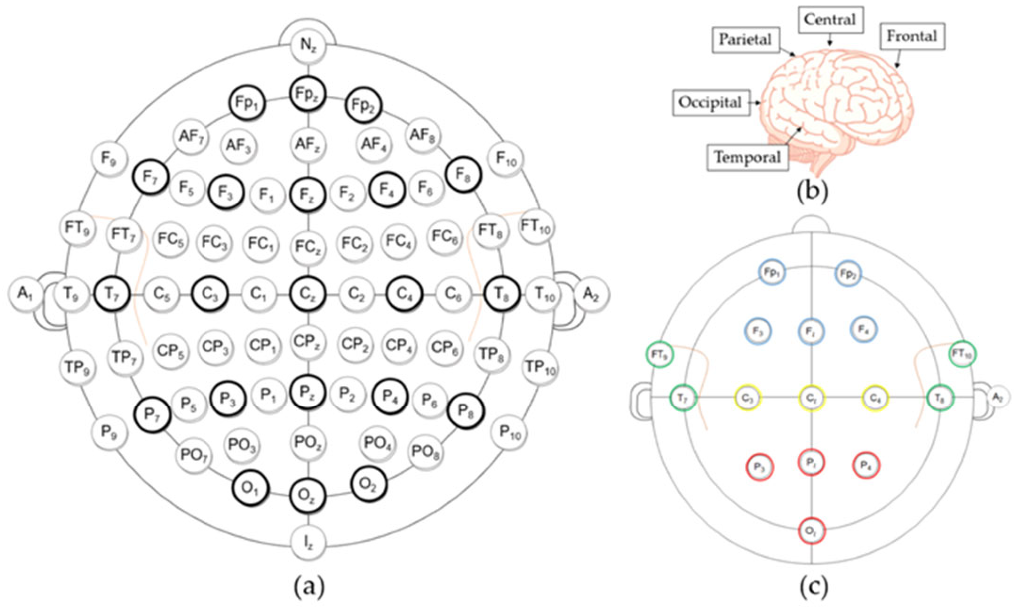
Electrodes can be positioned in different regions of the brain to extract relevant information. Such information can be used or interpreted into different classes. Some datasets consist of two classes, which represent left-hand movement and right-hand movement. Others consist of four classes, which represent right-hand movement, left-hand movement, tongue, and foot.
The BCI competition IV 2a [27] dataset consists of 22 motor imaging datasets. The data was collected from nine healthy individuals, focusing on four classes: left-hand, right-hand, foot, and tongue imagery movement. The dataset was bandpass-filtered between 0.5 and 100 Hz and further processed to focus on the 4–38 Hz frequency range at a sampling rate of 250 Hz. For uniformity, an exponentially shifted window with a decay factor of 0.999 was applied to each electrode signal. Each trial lasted 6 s, but only the segment between 0.5 and 2.5 s after the first stimulus was used for analysis, as this is when motor imagery activity is most prominent. In total, each participant contributed 288 trials. The dataset was divided into training and testing sets, with a portion of the training data used for validation during model development. The researchers employed a novel approach that combined EMD and fed it to PCNN for feature classification, aiming to enhance classification accuracy and robustness.
BCI competition IV dataset 2b, consisting of nine EEG participants, was used in this study as well. The dataset consisted of five sessions, with feedback provided only for the first two sessions. Participants were given a fixed cross and an auditory warning tone at the beginning of each trial. Within four seconds, they had to picture matching hand gestures.
Three bipolar recordings were made at a sampling frequency of 250 Hz, using a 50 Hz trap filter and a bandpass filter. Experiments on motor imagery tasks for both left- and right-handed motions were included. The data collection included 120 trials per session, separated by a minimum of 1.5 s of rest.
The study by [28] classified left and right MI EEG signals using the BCI competition IV dataset 2a and 2b. The dataset was used to provide EEG signals from all nine subjects, with five sessions provided for each subject. The data were recorded from three bipolar channels, including C3, Cz, and C4, with a sampling frequency of 250 Hz. The method was evaluated using data from C3 and C4 channels related to sensorimotor areas. For training, a single session, A03T, was used, while for evaluation, two sessions, A04E and AQ5E, were used. The LDA classifier was trained using 100% of the data from B0P03T and tested on 100% of the data for each of the sessions, B0P04E and B0P05E. The LDA classifier was trained and tested using features corresponding to EEG signals from a 3 s to 8 s time interval of the IM paradigm. The mean frequency of each IMF of EEG signals corresponding to left- and right-hand MI tasks was computed, and enhanced EEG signals were selected with mean frequencies falling in the range of 6–24 Hz. The Hjorth parameters and both powers were calculated for the enhanced EEG signals obtained using the results.
Zhang et al. [29] compared the performance of a neural network model with that of other state-of-the-art algorithms using two publicly available datasets from BCI competition IV. The dataset contains EEG and EOG signals from nine subjects, with each subject performing four classes of MI tasks. The four-class dataset comprises 72 trials per class, each with a motor imagery period of 3 s. To ensure the model’s performance, modifications were made to the signal input of the dataset. For dataset 2b, the number of trials in the last three sessions was doubled, resulting in 1200 trials for every subject, with each trial lasting 3 s. The total number of trials varied across different subjects, and the training and testing data were set at a 3:1 ratio. It also takes less than 0.025 s to test a sample suitable for real-time processing. The classification standard deviation for the nine different subjects achieved the lowest values of 5.5 for the 2b dataset and 7.1 for the 2a dataset.
Wang et al. [30] utilized MI-EEG data from the BCI competition IV dataset 2a and 2b to investigate motor imagery tasks performed with the left and right hands. The BCI competition IV dataset 2a collected EEG signals from 22 electrodes and recorded the locations of three EOG scalp electrodes for nine subjects. Participants were asked to perform four different motor imagery tasks involving the left hand, right hand, foot, and tongue. The study used data from motor imagery tasks involving the left and right hands. Before each session, a 5 min EOG recording was performed to eliminate eye movement artifacts. Participants were required to fixate on the screen for 2 s before engaging in 4 s of motor imagery. A sampling frequency of 250 Hz, a bandpass filter of 0.5–100 Hz, a sensitive amplifier of 100 µv, and a 50 Hz notch filter were used. A total of 22 scalp electrodes based on the international 10–20 system were used in the experiment. The experiment performance was average for both BCI competition IV 2a and BCI competition IV 2b, using an SVM classifier with features extracted from the combined CPS and PSD.
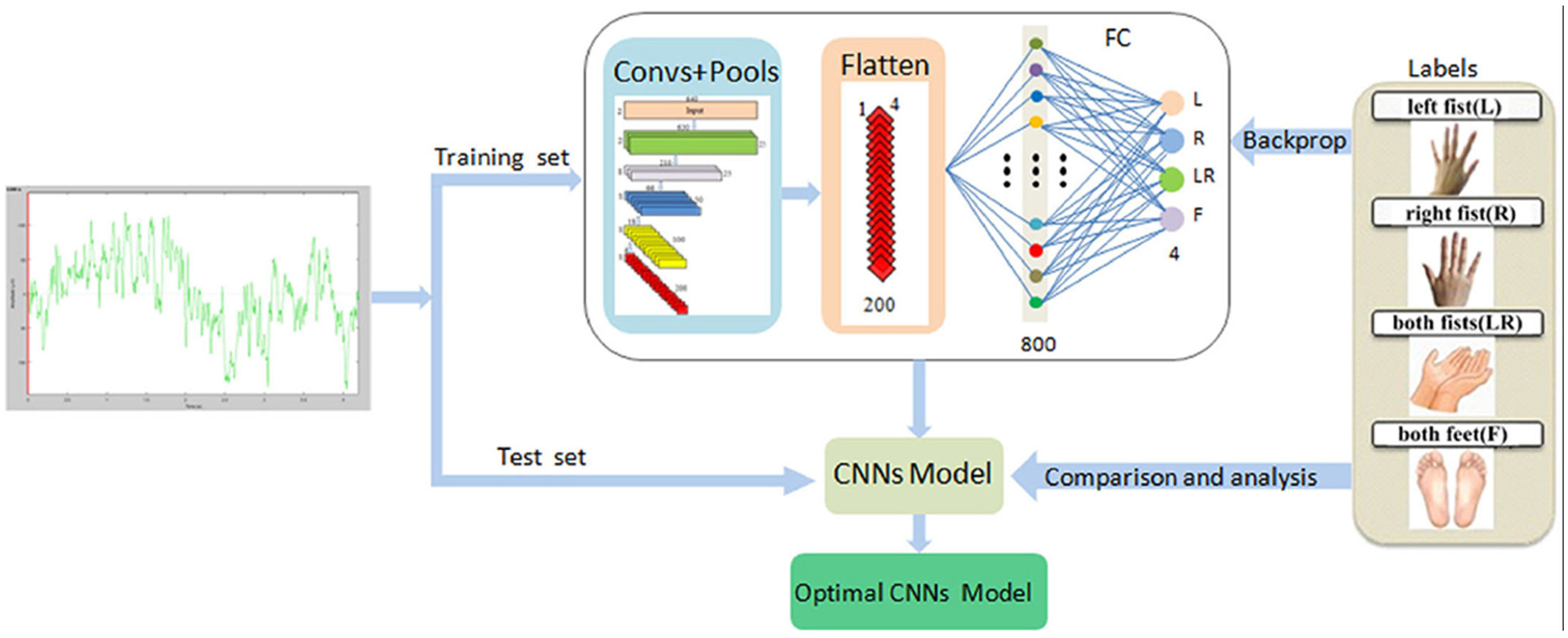
In the study by Chowdhury et al. [31], a model for motor imagery was proposed and tested using the Physio Net EEG motor movement/imagery dataset, which contains 1500 one- and two-minute EEG recordings from 109 subjects. The BCI2000 system was used to record EEG data during motor imaging activities. Participants completed 14 experimental runs, including 2 baseline runs with their eyes open and closed, as well as a three-minute run involving tasks of executing or imagining the opening and closing of the left or right hand, both fists, or both feet. For validation, two subgroups of the dataset were used, left-hand and right-hand movement tasks, as well as imaginary left-hand and right-hand movement tasks. Motor movement or imagery tasks were recorded as EEG signals on 64 channels placed on the subject’s scalp, annotated with three codes: T0, T1, and T2. To maintain dataset consistency, 4 s of data was clipped on each trial, sampled at 160 Hz, resulting in a total of 64 samples. The sliding window approach was used to divide the 640 into eight non-overlapping windows of 80 samples each, providing more discriminatory information on the motor imagery data. The signal processing module in the Gumpy BCI library was utilized to handle the EEG signals by applying a notch filter to remove mains (AC) interference at 60 Hz and using a fifth-order Butterworth bandpass filter to retain frequencies between 2 Hz and 60 Hz. The dataset was used to categorize actual and imagined movements made with left and right hands. The proposed model was slower, taking 361 ms and 354 ms of computational time per sample for real and imagined movements, respectively. This paper presented a multi-branch 2D-CNN model that processed EEG representations from separate electrode groups and frequency bands, which increased the computational demand but allowed the model to learn both spatial and temporal dependencies in parallel, thus improving discrimination between real and imagined motor tasks. R. Lv et al. [32] conducted the same study at a sampling rate of 160 using the same dataset and test experiment, with 10 and 30 subjects selected for experiment validation. The study focused on motor imagery tasks, divided into three experimental sections, each containing four tasks. To obtain high-quality EEG data, a fourth-order zero-phase Butterworth bandpass filter was used to preserve the original information. The data was then sliced into 0.4 s sliding windows with 0.4 s steps. The two-class and four-class subnets were formulated for each subject. Alomari et al. [33] experimented with two-class motor imagery when classified with SVM using features extracted from CSP with a processing time of 8.3 s per event.
Tibrewal et al. [34] presented a study that involved 57 subjects who performed a two-class MI task using an existing BCI system. The collected EEG signals were used to train a CNN and CSP + LDA model for offline classification. All subjects were right-handed and novices to BCI and MI. They received explanations and signed consent forms before the experiment. Sixteen electrodes recorded EEG signals from the sensorimotor area, using the 10–20 international system. The right earlobe was used as the reference electrode, and a ground electrode was set at AFz. A conductive gel was applied to maintain the impedance of the electrodes below 50 kOhms. The signals were amplified by a Nautilus amplifier and sampled at a rate of 250 samples per second. Noise during EEG recording was reduced by applying a 48–52 Hz notch filter and a 0.5–30 Hz bandpass filter. Participants performed 120MI trials, each lasting eight seconds. Each trial began with a fixation displayed in the center of the screen for 3 s, followed by a red arrow cueing the direction of the trail. The rest time between trials varied randomly between 0.5 and 2.5 s. Three participants’ signals were not recorded satisfactorily due to technical issues during the experiment, so only fifty-four participants were analyzed. An epoch of 4 s was selected from each trial. Figure 2 is the graphical representation of classification performance based on the dataset used for each study.

2.2. EEG Data Processing Pipeline for BCI Systems

Figure 3 shows the development of BCI systems from classic (1990–2005) to the current (2005–2012) and modern (2015–2025) approaches. Classical BCIs use simple EEG acquisition and basic pre-processing along with synchronous paradigms like motor imaging and P300 tasks. Current BCIs have evolved with improved signal processing pipelines, including adaptive filtering and hybrid extraction of features, as well as more reliable classification methods. Modern BCIs are expanding the pipeline further with deep learning, real-time artifact removal, hybrid paradigms, and adaptive decoding in assistive technologies that will provide a more accurate and flexible interpretation of user intent [36,37].
Signal processing techniques are essential in developing BCI systems by preparing EEG signals for analysis. These methods are efficient, easy to understand, and suitable for smaller datasets. However, EEG can be affected by noise, so careful processing is necessary to remove distractions and highlight important features. A successful BCI relies on good processing methods and the user’s ability to produce clear, reliable brain signals. The typical EEG BCI pipeline is shown in Figure 4. Signal acquisition is the process of collecting brain electrical activity for further processing. Signal preprocessing, is for removing noise and artifacts such as eye blinks and muscle movements to improve signal quality and SNR, leading to a better accuracy [38]. Feature extraction identifies meaningful patterns in EEG data to reveal brain activity associated with specific thoughts/intentions, and classification for converting brain signals into commands that a system can understand.

2.2.1. Preprocessing and Decomposition

EEG-based BCI filtering is a crucial stage that influences the quality of subsequent processing. EEG recordings, while capturing brain activity patterns, also gather various unwanted noises originating from environmental factors, the recording equipment, and even the subject’s physiological movements. Filters play a critical role in this context by selectively eliminating frequencies that do not correlate with brain activity while preserving those that are rich in useful information. Filters work by filtering out all unwanted frequency noise and retaining only the brain rhythms within a specific frequency range [40]. The goal is to preserve neural information like mu (8–13 Hz) and beta (13–30 Hz), while eliminating artifacts such as slow drift (<0.5 Hz), power lines at 50/60 Hz, and muscle activity (>40 Hz). These rhythms carry the key neural information needed for tasks such as imagining movements. Equation (1) shows the mathematical expression for a bandpass filter, as the convolution of the raw EEG signal with the impulse response of the filter:
y t = x t h t
where
  • x t is the recorded raw EEG signal.
  • h t is the impulse response of the filter.
  • y t , the filtered signal output, is only the frequencies of interest.
Design characteristics determine whether decomposition and feature extraction methods operate on meaningful brain activity or noise-contaminated signals. The filter order affects the distinction between the passband and stopband, with higher orders requiring a narrow mu rhythm but increasing latency, which is undesirable in online BCIs. The transition band is also crucial, as a wide boundary between preserved and attenuated frequencies can blur distinctions between alpha and low-beta rhythms, affecting classifiers’ usability [41]. Ripple, small fluctuations in passband or stopband gain, can distort amplitude estimates and bias power spectral density, while poor stopband attenuation can mask subtle neural modulations due to residual 50 Hz interference. Choosing the right frequency ranges for BCI application means matching them closely to the brain’s natural rhythms. Usually, this involves focusing on the 8–30 Hz range to capture sensorimotor activity and using notch filters around 50/60 Hz to block out electrical noise from power lines. This is achieved without affecting the rest of the EEG signal, as shown in Equation (2), with f 0 being the frequency to suppress:
H f = 0 ,     i f   f = f 0 1 ,   o t h e r w i s e
To approximate f 0 , digital filters are used; this can be implemented using a Notch IIR filter:
  y n = x n 2 cos 2 π f 0 f s . x n 1 + x n 2 + a 1 y n 1 + a 2 y n 2
  • x n is the input signal (with noise);
  • y n is the output (filtered EEG);
  • f 0 is the notch frequency;
  • f s is the sampling rate;
  • a 1 , a 2 are the feedback coefficients used to shape the EEG signal.
Getting these frequency bands right is important because if they are too broad or narrow, you might lose important brain signals or let in unwanted noise, which can degrade system performance. Another important factor is the windowing function used in designing FIR filters. Hamming windows reduce signal leakage, while Kaiser windows provide more control for fine-tuning filter performance.
It is also important to find balance between preserving the accuracy of brain signals and keeping the processing efficient. Karpiel et al. [42] highlighted that different filter types (FIR, IIR, FFT, and notch filters) can have a big impact on the timing and strength of brain signals related to movement control, especially within a critical time window of approximately 100–300 ms. Vasei et al. [43] discovered that FIR filters are often favored in wearable BCI devices because they do a better job of blocking unwanted frequencies outside the key sensorimotor rhythm range. However, these filters need more processing power. FIRs are used to calculate the value of the correct output using a finite number of past input data, as shown in Equation (4). This type of filter is suitable for a linear phase response.
y n = k = 0 N b k . x n k
y [ n ] is the current output, x [ n k ] is the past input samples, b k is the filter coefficients (impulse response) and N is the filter order. IIR filters, on the other hand, use less computational resources and are good for real-time use, but can cause distortions in the timing of brain signals. This timing distortion can affect later analysis steps such as ICA or feature extraction, which rely on precise signal timing for accurate interpretation. An IIR filter uses both past input and output values to generate the value of the correct output y n ; it does this using a few coefficients [44]. Equation (5) depicts the mathematical expression for finding both past inputs and output values to generate correct output values.
y n = k = 0 M b k . x n k l = 1 P a l . y n l
with x n k being the current and past inputs and y [ n l ] representing past outputs. One of the drawbacks of using IIR is that it introduces a nonlinear phase shift. One of the commonly used algorithms in adaptive filters is LSM (Least Mean Square), expressed in Equation (6). This type of method learns and adjusts to brain patterns by minimizing the difference between reference input (the desired output) and the actual noisy signal (what you receive), making it ideal for real-time processing [45]. LSM achieves this by learning artifact patterns (EOG, MEG, etc.) and subtracting them out in real time without degrading signal integrity.
w n + 1 = w n + µ · e n · x n
where
  • w n is the learned filter;
  • µ is the learning rate;
  • e n is the error between the desired clean signal and the current output;
  • x n is the current input signal (with noise).
Following the noise removal by filtering, the brain signals and artifacts can overlap, and the decomposition methods are utilized to separate the signals and artifacts for preparation.

2.2.2. Decomposition

Decomposition is a crucial step in EEG data analysis after filtering to remove noise. EEG recordings capture activity from many overlapping processes, such as brain responses, muscle movements, and eyeblinks; it becomes difficult to see which part of the signals are actually linked to the task being studied. It helps separate mixed signals from physiological interference and other brain processes. Decomposition methods help researchers understand the signal better and extract significant aspects that accurately reflect brain activity associated with a task. This process separates task-related brain signals from overlapping noise and artifacts, preparing data for precise analysis and interpretation in BCI research [46].
ICA and its more advanced features, such as AMICA, are key techniques used in EEG signal processing [47]. These methods work by separating the recorded signals into statistically independent sources. This separation is especially helpful because it allows researchers to identify components dominated by artifacts, such as eye blinks or muscle movements, and remove them without affecting the true brain activity [48]. ICA shown in Equation (7) is based on the assumption that EEG x(t) is the mixture of sources s(t), the original signal from the brain, and A, the unknown mixing matrix that is represented as shown in Equation (8):
x t = A · s t
Unmixing matrix (W) can be represented as
x t = W · x t
Similar to ICA, AMICA assumes that EEG data is the product of many models and hidden sources, which contribute to the total EEG data. Equation (9) can be used to calculate the total EEG data:
x t = A m · s m t     f o r   m = 1,2 , 3,4 , 5 ,   M
A ( m ) is the mixing matrix for the model m , s m ( t ) are the source signals under that model, and M is the total number of adaptive mixture models. AMICA adjusts to the signal’s change by analyzing multiple models and selecting the most suitable one for the signal at each time step. This decomposition step is critical since, without it, machine learning models might mistakenly focus on these noise patterns instead of genuine neural signals, reducing both the accuracy and reliability of the results [49]. Properly applying ICA ensures that the features learned truly represent brain function, improving the overall performance and generalizability of BCI and other EEG-based studies.
Time–frequency decomposition plays a vital role in analyzing EEG signals, especially because brain activity is often fleeting and changes rapidly over time. Techniques like wavelet transforms are popular because they allow researchers to look at both when and at what frequency certain brain rhythms occur during a task. Choosing the right wavelet, such as Daubechies or symlets, affects how well the signal is smoothed and localized. Symlets are a more symmetrical form that is helpful when the phase is crucial, whereas Daubechies (db4, db8) are tiny and smooth for EEG signals. Also, selecting the appropriate number of decomposition levels is crucial, although more levels may expose more intricate information. They may also add excessive complications. Another key consideration is whether to use continuous wavelet transform (CWT), which offers detailed resolution but demands more computing power, or the discrete wavelet transform (DWT), which is faster and better for real-time BCI [50]. Equation (10) is a discrete wavelet transform where the signal x ( t ) DWT is represented as
x t = k a j 0 , k · φ j 0 , k t + j = j 0 J k d j , k · ψ j , k t
where φ j 0 , k t is the scaling function at level j 0 , ψ j , k t is the wavelet function and a j 0 , k and d j , k are wavelet coefficients at level j and position k . Approximation components are shown in Equation (11), and the detail component is shown in Equation (12)
j , k t = 2 j 2 · 2 j t k  
φ j , k t = 2 j 2 · φ 2 j t k
Approximation and detail coefficients can be calculated by breaking down data into various resolutions using the basis function presented above.
EMD and its weighted form, WMD, are flexible techniques that separate EEG signals into simpler components called intrinsic mode functions [51]. This can be represented mathematically by using Equation (13), assuming that x(t) is the original EEG signal. They perform this without relying on predetermined patterns. These methods are especially good at picking up subtle and complex changes in the brain activity. However, they sometimes face challenges such as overlapping components (mode mixing) and difficulty in producing consistent results every time. Despite these issues, EMD and WMD are very useful after the initial filtering step because they uncover detailed temporal patterns that basic bandpass filters often miss [52,53]. These deeper insights help researchers extract richer features and better understand brain function. Preprocessing and decomposition are crucial stages in BCI systems, laying the foundation for feature extraction and classification.
x t = k = 1 K I M F k t + r t
with I M F k ( t ) being the K-th intrinsic mode function, r ( t ) being what is left after decomposition, and K being the number of IMFs. WMD can be mathematically expressed as shown in Equation (14), where WMD breaks down the original signal into a sum of wavelet-based modes:
x t = k = 1 K W M k t
With the use of specifically created wavelets that capture certain frequency bands, the derived wavelet modes through bandpass filtering are mathematically described as the k t h mode:
W M k t = x t φ k t
φ k t is the wavelet function tuned to the k t h frequency band.
For increased efficacy, VMD can be used in conjunction with other methods [8,54]. Let us express it mathematically using Equation (16), where
x t = k = 1 K u k t
A complex-valued u k t is the representation of the instantaneous phase and amplitude of each real-valued mode, as shown in Equation (17), obtained by converting it into its analytic signal using the Hilbert Transform:
u ^ k t = δ t + j π t u k t
To demodulate each mode (shift to baseband) at the center frequency to obtain the bandwidth easily, Equation (18) is applied first.
u ^ k t · e j w k t
Then, the bandwidth of each mode is computed using the squared L 2 energy of the gradient, obtained by Equation (19):
t [ u ^ k t · e j w k t ] 2 2
The goal is to achieve a small ‘’wide’’ mode by measuring the frequency width of the mode to decrease its overall bandwidth, and minimize the total bandwidth by
m i n u k , { w k k = 1 K t δ t 1 + j π t u k t · e j w k t 2 2
Equation (20) can be calculated under the following condition:
k = 1 K u k t =   x t
When all modes are mixed, the constraint guarantees that the original EEG signal x t shown in Equation (21) is recreated.
A Multivariate EMD (MEMD) technique separates frontal EEG channels from mental state using electrode decomposition across electrodes. MEMD demonstrated its capacity to detect oscillatory information that can be missed when using standard Fourier or wavelet analysis in one of the 2022 BCI studies, with an outstanding accuracy of 98.06%. When intense artifacts are present, classic EMD may experience mode mixing, which typically occurs when distinct neural rhythms are combined into a single IMF or when a single rhythm is divided across several IMFs. This can be addressed by applying Complete Ensemble EMD with Adaptive Noise (CEEMDAN), which introduces controlled noise during decomposition. Hu et al. [55] recently presented a hybrid DWT-CEEMDAN-ICA pipeline in 2022 to deal with a single-channel EEG that has eye-blink artifacts. This hybrid approach detected and eliminated ocular components without overcomplete problems using ICA with sample entropy, performed CEEMDAN to prevent mode mixing, and expanded the signal using the discrete wavelet transform (DWT). BCIs rely on preprocessing and decomposition stages for feature extraction and classification. When designed carefully, these stages enhance the signal-to-noise ratio and reveal neural dynamics. Decomposition methods bridge clean signals with meaningful features, ensuring noise-free and representative neural processes. However, poorly designed filters can distort input, and careless choices in decomposition parameters can obscure or fragment task-relevant rhythms.

2.3. Feature Extraction and Spatial Enhancement

EEG signals undergo a crucial stage of feature extraction and spatial enhancement after filtering and decomposition. This stage focuses on identifying patterns that differentiate mental states. Feature extraction pulls out meaningful brain patterns from EEG data to identify brain activity related to specific thoughts/intentions; it converts complex brain activity into simpler representations, using measures like PSD shown in Equations (22)–(24) and Hjorth parameters (activity, mobility, and complexity) in Equations (25)–(27), to capture changes in signal behavior over time [56]. Given an EEG signal x(t) in Equation (22), one may segment and window the signal by dividing it into shorter overlapping segments and applying a window function to minimize the edge effects.
x k w t = x k t · w t
Apply the Discrete Fourier Transform for each segment to convert it into the frequency domain using Equation (22):
X k f = t = 0 N 1 x k w t · e j 2 π f t / N
In order to obtain the PSD estimate, we need to average over the segments by using Equation (24):
P S D f =   1 K k = 1 K P k f
Hjorth parameters are simple yet effective in characterizing the complexity and nature of EEG signals, especially useful in BCI, a system that distinguishes between multiple mental activities [57].
A c t i v i t y = V a r x t
Activity provides insight into the brain response intensity during a mental task, as calculated in Equation (25).
m o b i l i t y = V a r x t V a r x t
c o m p l e x i t y = M o b i l i t y x t M o b i l i t y x t

Hjorth Parameters

The temporal domain features of EEG signals are described statistically by Hjorth parameters. They evaluate the signal’s level of intensity, frequency, and waveform fluctuation over time. Beta activity is associated with motor planning or the region of interest, and increased mobility is a sign of this activity. Complex signals can be a sign of increased imagination or cognitive processing that can be obtained by applying Equation (27).
Techniques like CSP improve how well we can tell apart different brain states by creating spatial filters that emphasize the differences. It is mathematically expressed in Equations (28) and (29). However, these methods rely on the quality of earlier steps, as unprepared signals may mirror noise instead of real brain activity. Spatial enhancement techniques improve how EEG signals are represented across multiple channels by reducing noise and influencing neighboring electrodes [22]. One popular technique for calculating spatial filters to detect ERD/ERS effects and ERD-based BCIs is the typical spatial pattern (CSP) algorithm. It identifies the routes that increase variation for one class while minimizing variance for another. Once the EEG data have been bandpass-filtered in the frequency domain of interest, a high or low signal variant indicates strong or weak rhythmic activity [58]. When left-hand movements are envisioned, a signal from a particular filter centered on the left-hand area exhibits an attenuated motor rhythm. Still, when right-hand motions are imagined, the signal shows a strong motor rhythm.
CSP, Laplacian filtering, and advanced Riemannian geometry methods amplify signals related to a task while reducing noise, which can be mathematically expressed as shown in Equations (30) and (31). This ensures features carry frequency and spatial information. When combined with spatial enhancement, raw brain signals become clear, structured data for machine learning algorithms to interpret. Poor preprocessing or weak feature design can limit how well classifiers work, but when done well, they significantly improve the accuracy and reliability of BCI [59].
w = arg max w T C 1 w w T C 1 + C 2 w  
Projected signals:
Z t = w T x t
where x ( t ) is the EEG signal at time t .
y i t = x i t 1 N   j ϵ N i x j t
d R C i ,   C j = log C i 1 2 C j C i 1 2 F

2.4. Machine Learning in the EEG-Based BCI

Traditional machine learning is crucial for classifying features from EEG signals after refinement. These techniques act as translators, setting boundaries within the processed data to assign meaningful categories. Their success hinges not only on having good-quality features but also on fine-tuning their parameters to balance flexibility and stability. Traditional machine learning focuses on developing algorithms for predictions or decisions, even with smaller datasets [60]. Common methods include support vector machine, random forest, KNN, and linear discriminant analysis, all of which identify patterns in the features to predict outcomes on new data.
LDA is a popular classifier in BCI research due to its simplicity and effectiveness. It assumes features follow a Gaussian distribution and projects data into a new space to clear differences between classes. However, LDA’s performance depends on careful tuning to avoid overfitting, especially when there are many features but limited data. SVMs can handle complex, nonlinear separations using kernel functions (linear, radial basis, polynomial), which help draw flexible boundaries with parameters that directly influence classification performance. Hyperparameters such as the kernel type, penalty parameter (C), and kernel width (y) directly influence classification accuracy [7].

2.4.1. Linear Discriminant Analysis (LDA)

For tasks involving dimensionality reduction and classification, especially two-class classification, LDA is a popular supervised learning technique. To efficiently divide classes, it statistically models feature distributions and determines the optimal linear combination of specified characteristics. The basic idea behind LDA for binary classification is to differentiate between two classes by considering that they have a normal distribution [61]. The offline dataset is subjected to this assumption by obtaining the covariance matrices and mean vectors for every class. The covariance matrix of both classes is similar. Data labels can be obtained using Equations (33) and (34) with respect to its normal vector w and bias b; the feature vector x’s distance from the separating hyperplane is denoted by the value D(x) [62]. The means of each class, µ1, µ2 and the inverse variance matrix 1 , can be used to describe the parameters w and b. The detected feature vector x is allocated to a class based on the sign of D(x).
D x = w T · x + b
w = 1 1 · µ 2 µ 1
b = w T · 1 2 · µ 1 + µ 2

2.4.2. Support Vector Machine

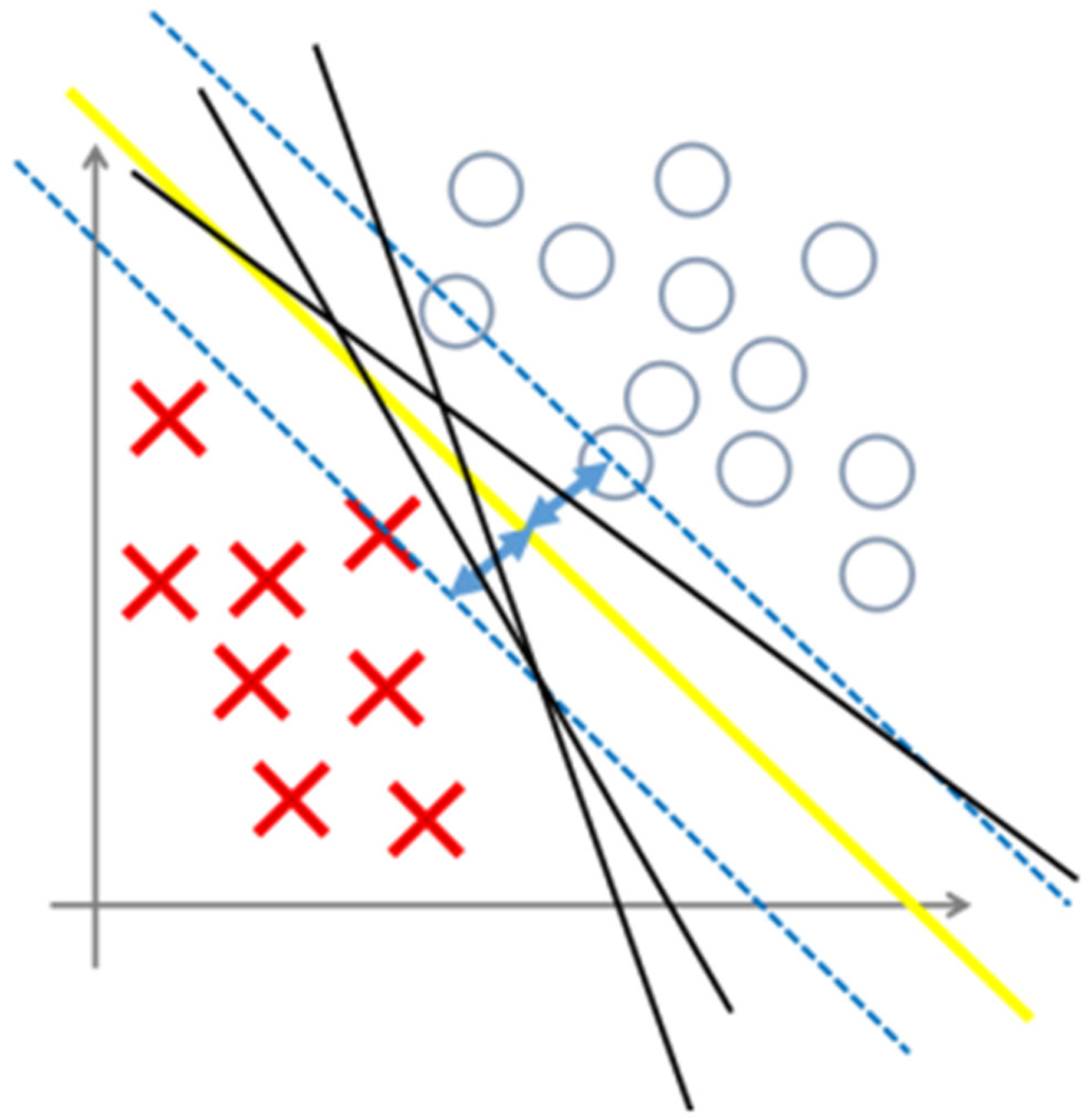
SVM is a linear classifier that divides data into high-dimensional spaces by assigning feature vectors to different classes using a hyperplane, as shown in Figure 5. BCI systems use their nonlinear classifier k(x,y), which has a high classification accuracy for tasks including pattern recognition, MI-based control, hand movement detection, and feature discovery from EEG data. With SVM, several synchronous BCI problems have been resolved [63]. In order to transform data to a higher-dimensional space for nonlinear decision boundaries, the ‘kernel trick’ uses a kernel function presented in Equation (35).
A popular kernel in BCI research is the Gaussian or Radial Basis Function (RBF) kernel. For BCI applications, SVMs perform well; however, some hyperparameters must be defined, including the regularization parameter C and the RBF width σ if kernel two is used.
K ( x , y ) = e x p x y 2 2 σ 2

2.4.3. K-Nearest Neighbors K-NN

One machine learning technique frequently applied in BCI systems is the K-NN algorithm. It uses an element’s value to determine which it belongs to. A predetermined parameter k determines the number of neighbors and has a direct impact on the classifier’s performance. The square root of the total number of samples is usually more than k. Methods such as the Manhattan, Minkowski, and Euclidean distances are used to determine the distance to the neighbors. Data points that have been broken into many classes are found using the K-NN method to predict the classification of a new sample point. It utilizes the training dataset to generate predictions after analyzing similarity using distance formulae [65]. Following a search for the K most comparable instances, the output variable for that instance is brought to the point in order to produce predictions for a new instance (x). The K instances closest to the new input are used to measure the distance, as obtained from Equations (36)–(38).
d x y = i = 1 k x i y i 2
d x y = i = 1 k x i y i
d x y = ( i = 1 k ( x i y i ) ) 1 q
Random Forests (RF) are a type of decision tree that enhances predictive performance by creating an ensemble of multiple trees, as shown in Figure 6. The effectiveness of a random forest model depends on several critical hyperparameters, including the number of trees, the maximum tree depth, and the feature selection method. These hyperparameters influence the model’s ability to capture genuine patterns in the data or overfit to noise. Researchers can use manual tuning or automated strategies, such as grid search or advanced Bayesian optimization, to tune these hyperparameters. Both manual and automated adjustments help find the best settings and reduce bias [66]. Equation (39) represents the majority voting rule.
( x ) = arg m a x y ϵ γ j = 1 J I ( y = h j x )
where
  • h j x is the prediction of the j-th decision tree.
  • J is the total number of trees in the forest.
  • I ( . ) is the indicator function (1 if true, 0 if false).
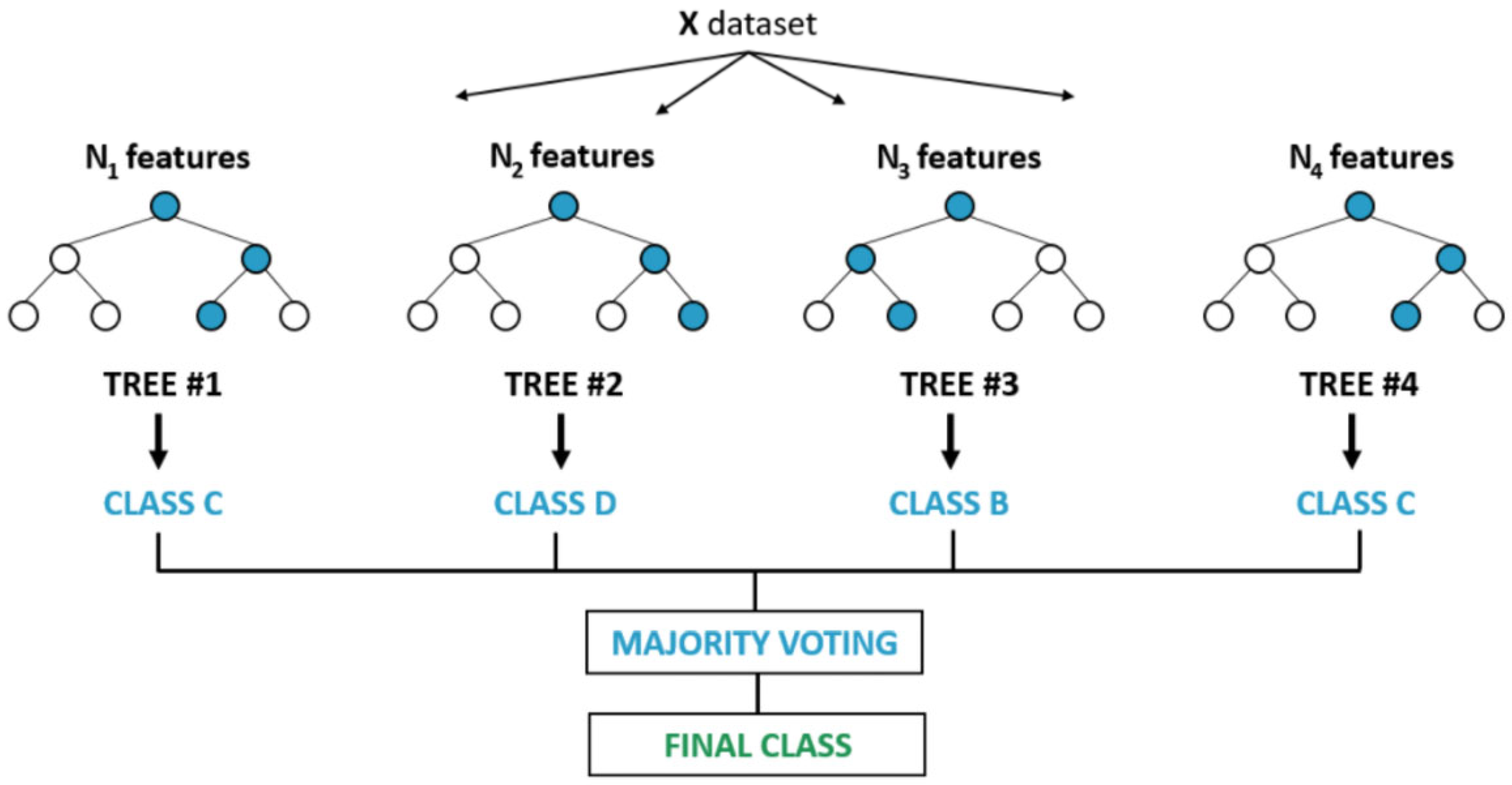
The class with the most votes across all trees is chosen as the final prediction.
Figure 6. RF process, where multiple decision trees independently classify the input EEG feature vector, and the final class label is determined by majority voting across all trees [67]. # refers to a number.
Applsci 15 12075 g006
Machine learning classifiers’ effectiveness relies on the quality of features they analyze and the tuning strategies used. CSP features complement linear classifiers like LDA, while nonlinear features like wavelet coefficients perform better with kernel-based support vector machines (SVMs). Understanding the entire processing pipeline is crucial for feature extraction, machine learning success, and accurate user intention interpretation.
This relationship highlights the importance of understanding the entire processing pipeline. Since poor preprocessing can hinder feature extraction, weak features limit machine learning success, and improperly tuned classifiers reduce the ability to accurately interpret user intentions. As brain signal complexity increases and manual design of feature-classifier combinations becomes less practical, there is a shift towards deep learning methods. Deep learning integrates feature extraction and classification into a unified system, offering a powerful alternative for handling complex data.

2.5. Deep Learning Models in the EEG-BCI Pipeline

The transition from traditional machine learning (ML) to deep learning (DL) in EEG-based BCIs was driven by challenges in earlier methods. Classical ML largely depends on handcrafted features such as PSD, Hjorth parameters, and CSP. Although these features have demonstrated effectiveness in specific contexts, they tend to be dataset-dependent and sensitive to noise. This makes their performance unstable when systems are transferred from controlled laboratory conditions to more variable, real-world assistive environments. DL emerged as a promising alternative by enabling modes to learn features automatically from raw or minimally processed EEG data. This not only reduces the reliance on handcrafted feature design but also allows the discovery of richer, nonlinear representations that classical methods often miss.
A wide range of DL architectures has been explored in this domain. For example, CNNs, RNNs, and hybrid models such as CNN-RNNs have been investigated for EEG analysis. CNNs record spatial–temporal patterns across EEG channels, making them particularly effective for motor imagery tasks, where oscillatory rhythms are distributed over multiple cortical regions [68]. RNNs and especially LSTM networks are more suited to capturing temporal dependencies by modeling sequential activity, such as event-related desynchronization and synchronization. More recently, GNNs have been proposed to explicitly incorporate electrode topology and functional connectivity, offering a more structured way of representing EEG dynamics. DL is effective due to its design and tuning of models. Critical hyperparameters such as learning rate, number of layers, convolutional kernel size, and dropout probability directly impact the model’s ability to generalize without overfitting [69].

2.5.1. Convolutional Neural Network

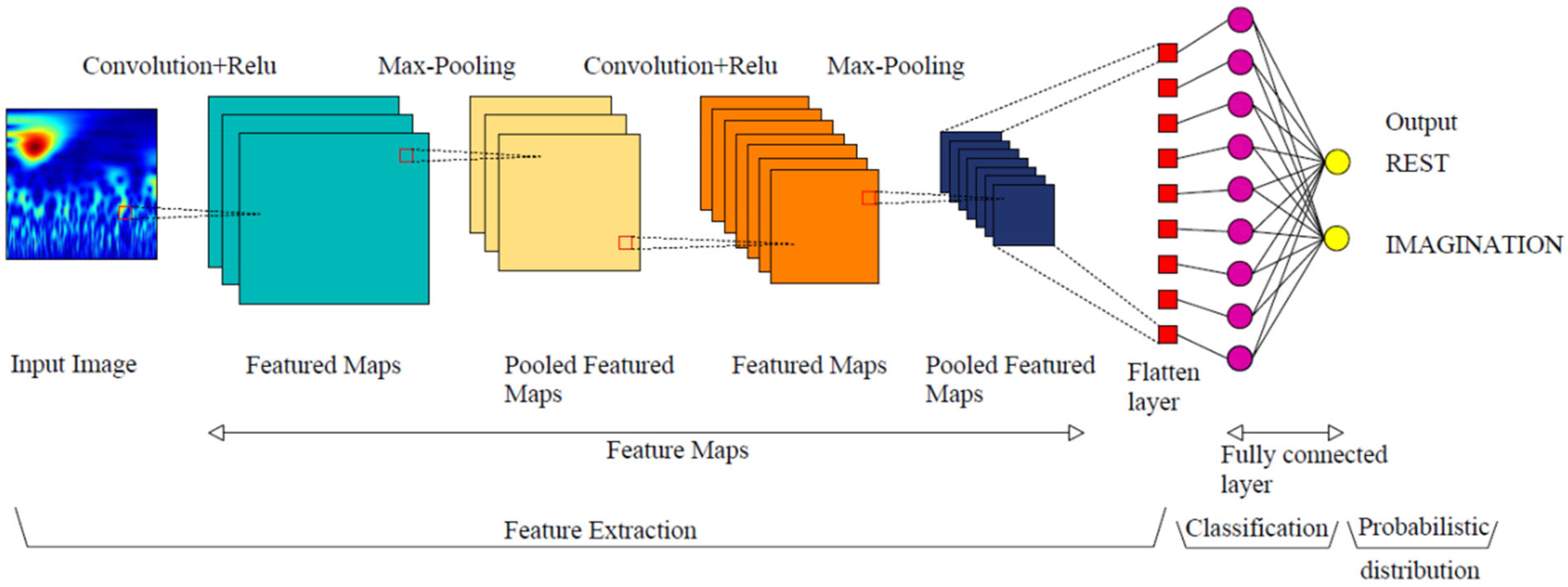
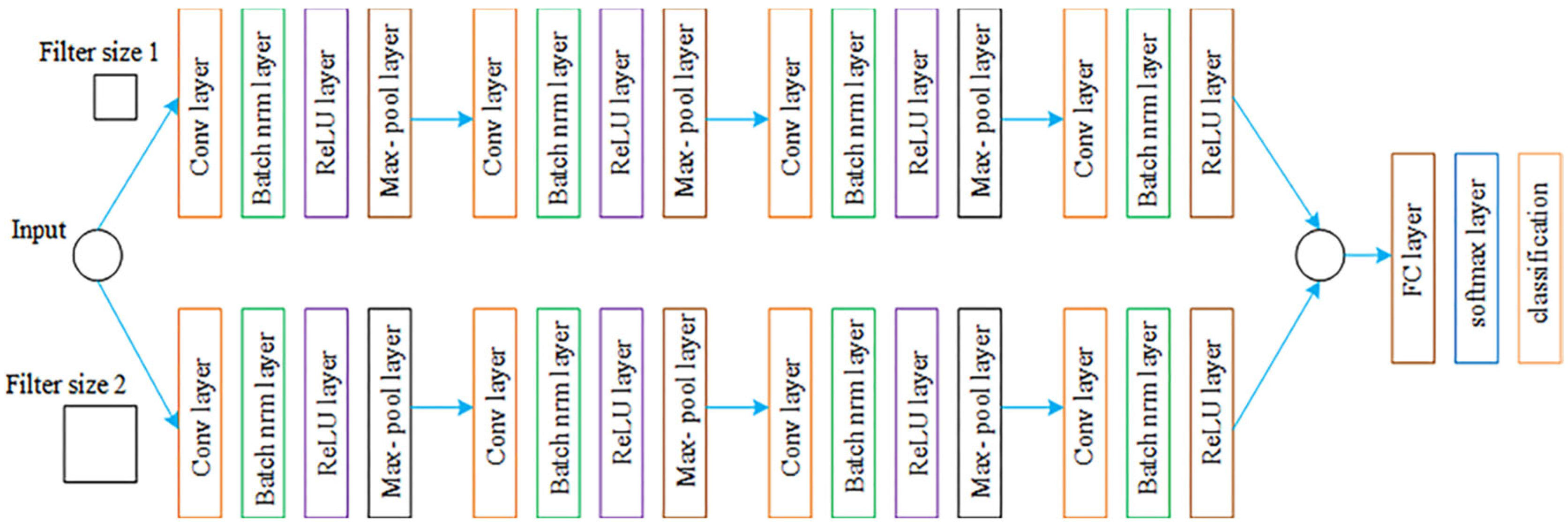
Since the recorded signals are complicated and noisy, CNN algorithms are crucial for classifying EEG signals. Raw EEG data contain several concurrent activities in the brain; hence, pre-filtering is essential to improve classification performance. CNNs are made up of fully connected layers, pooling, activations, and convolutional filter layers. Pooling reduces parameters and mitigates overfitting by efficiently downsampling data. While filters help learn abstract structures and expand the feature space, convolution layers extract features from the data matrix. Incorporating fully connected layers into a convolutional layer’s output facilitates the learning of nonlinear combinations of high-level features. Nonlinear plots of EEG data recorded in microvolts are represented by EEG channels, which show changes in magnitude over time. Often, the frequency content is displayed on one axis while the whole input signal is converted into a sequence of 2D time–frequency pictures. X. Lun et al. [69,70] introduced a five-layer CNN structure, as depicted in Figure 7, which utilizes a fully connected layer for classification and a four-layer maximum pooling to categorize physiological activity. Methods of batch normalization and dropout were used to reduce the risk of overfitting.
To detect motor activity, Zhang et al. [71] broke down EEG data using the short-time Fourier transform (STFT) approach. With the SoftMax classifier, the resultant data was fed into a seven-layer CNN with several core layers, such as 100 and 2 neurons. The weight matrix used to filter the input data represents the kernel size, a crucial hyperparameter for CCN tuning. Larger kernels detect low-frequency objects, while small filters detect high-frequency objects. Since the EEG is nonlinear and non-stationary, it is difficult to perform a thorough analysis. Consequently, choosing the kernel filter size is essential and ought to be handled as though it were stationary throughout a given period. Inception is a new layer design that researchers developed to solve this problem—using filters of different widths, including convolution and combination. Figure 8 shows the layer structure of the CNN model and shows how the dimensions of the feature map change as the data moves through the network. The model uses 3 × 3 convolution kernels with 1 × 1 spacing and equal padding to maintain spatial dimension, with a layer size of 2 × 2, gradually decreasing from 256 × 256 × 16 to 128 × 128 × 16 and finally 64 × 64 × 32. These extracted properties are then flattened and passed through fully connected and SoftMax layers to be classified in two classes (Rest and Imagination). This design enables the network to capture both fine and large spatial features of EEF data efficiently, improving its ability to differentiate between different motor imagery states.

2.5.2. Parallel Convolutional Neural Network

A neural network that processes input data in parallel across several computing units or devices is a Parallel Convolutional Neural Network (CNN). Multiple convolutional layers or operations can be carried out concurrently using CNNs, resulting in quicker processing times and increased efficiency compared to traditional CNNs that apply convolutional layers sequentially. One of the main parts of a parallel CNN is the convolutional layer, which extracts features from the input data by using a series of learnable filters [73]. Data and model parallelism can be accomplished via parallel CNNs, which divide input data across several processing units and execute identical actions concurrently. This is illustrated in Figure 9, showing parallel CNN layers. Faster training and inference are made possible by their frequent deployment on multi-GPU or multi-core systems, which take advantage of parallel processing capabilities [27].
In situations where data or model parameters must be synced across multiple devices, parallel CNNs require effective communication and synchronization protocols. By utilizing more processing resources, parallel CNNs provide scalability advantages that allow them to manage larger datasets and more intricate models. The MI-EEG BCI system is based on a one-dimensional convolutional neural network (1D-CNN) and takes as input a matrix of dimensions M × N.
Unlike ML, DL frameworks now rely on automated optimization techniques, making the tuning process more systematic and scalable. Techniques like Bayesian optimization, adaptive gradient techniques, and population-based training reduce the researchers’ dependence on subjective decisions. DL has resolved several issues with the BCI pipeline, such as learning directly from raw data, improving feature robustness, and enabling generalization across subjects and recording sessions. Hierarchical representations capture both local and global signal dynamics, and DL simplifies information loss at every level by integrating preprocessing, feature extraction, and classification into a single framework.
DL has shown significant improvements in intention detection rates, making it a crucial element in modern BCI systems, especially those designed for adaptive, real-world use. However, it faces challenges such as larger datasets, higher computational resources, and opaque decision-making processes, which raise concerns about interpretability in safety-critical assistive applications. Hybrid approaches aim to balance accuracy, robustness, and transparency by combining the representational strength of DL with the interpretability and efficiency of traditional techniques. These approaches aim to address the challenges of larger datasets, more processing power, and opaque decision-making procedures in assistive applications.

2.6. Hybrid Approaches in EEG-Based BCI Systems

Hybrid approaches in EEG-based BCIs aim to balance the strengths and weaknesses of deep learning by combining classical signal-processing techniques with modern deep architectures. These methods preserve interpretability and robustness while benefiting from the representational depth of neural networks. Traditional methods such as CSP, ICA, or wavelet transforms are used as front-ends to reduce noise and emphasize physiologically meaningful patterns. On the other hand, hybrid embedded machine learning classifiers like SVMs or RF within deep frameworks, leveraging their stability and interpretability to make the final decision layer more transparent. This approach aims to reduce data requirements and improve the structure of the deep model [74].
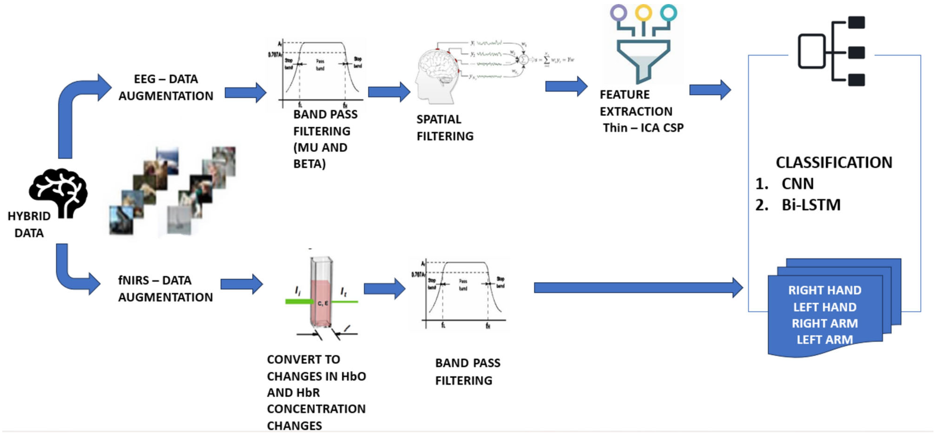
Hybrid EEG-based BCIs combine handcrafted features with deep learning to handle natural differences in tasks like motor imagery. This is illustrated in Figure 10. For example, in motor imagery tasks where brain activity varies greatly between individuals, handcrafted features help ensure stable performance across different users. This blend provides stability across users and captures complex brain activity patterns, enhancing performance and reliability in practical settings by adapting more effectively to each individual [70].
In non-stationary or real-world environments, hybrids allow for modular tuning, allowing preprocessing and feature extraction to be adjusted independently without retraining the entire pipeline. Recent studies have explored more efficient optimization by tuning the hyperparameters of both the feature extraction module and the deep learning model together [76]. Approaches such as Bayesian optimization and evolutionary algorithms automate this process, making hybrid systems not only more accurate but also faster and less demanding in terms of computational resources. Altogether, these features make the hybrid BCI pipeline highly effective and practical, especially in challenging scenarios where individual variability and changing environments are present. Their ability to combine robustness, flexibility, and efficiency highlights hybrid systems as a promising direction for advancing EEG-based BCIs.

3. Results

This section examines how various researchers have addressed the challenges in BCI systems using signal preprocessing and feature extraction methods. These methods are examined based on the machine learning and deep learning models, highlighting system performance. First, it reviews different methods used by researchers, highlighting their performance to analyze how different approaches influence EEG classification outcomes. It also evaluates how dataset characteristics impact overall system performance, as displayed in Figure 11. It should be noted that this section evaluates the performance of different methods reported by researchers in the existing literature.

3.1. Performance of MI Classification Methods

To enhance the resilience and classification accuracy of EEG data, Huang et al. [27] proposed a novel method that combines Parallel Convolutional Neural Networks (PCNN) with empirical mode decomposition (EMD). EMD was used to break down EEG data into intrinsic mode functions (IMFs), and PCNN was used to classify the features. The EMD-PCNN had a classification accuracy of 99.1% for four classes and 99.39% for two classes. Agrawal et al. [18] assessed the effectiveness of Deep Neural Networks (DNN) in classifying EEG signals using real-time processing and a hardware database that was constructed. Four types of data were used to represent the various brain states of individuals with neurological disorders. With an average classification accuracy of 97%, the DNN outperformed other techniques with which it was compared, with an accuracy of 85% in real-time processing. The proposed approach offers several key benefits, including a customized database, real-time processing, high classification accuracy, and superior real-time processing speed. The results are more pertinent and valuable as the hardware database that was constructed records more accurate and relevant EEG signals. With this novel method, EEG data processing is advanced, and new avenues for personalized, real-time neurological applications are opened up.
V.K. Mehla et al. [21] presented a technique for identifying EEG signals as either normal or those recorded during mental math exercises. From non-stationary EEG data, it extracts information such as Hjorth parameters, kurtosis, skewness, standard deviation, root mean square, and maximum value to create 10 intrinsic mode functions using the EMD approach. The characteristics are then fed into a classifier that uses support vector machines, which achieves a 95% classification accuracy. M.J. Antony et al. [20] compared adaptive support vector machine with Linear SVM, LDA and adaptive LDA, which resulted in an accuracy of 89%, 81%, and 86% respectively. Adaptive SVM had an accuracy of 91%. The system used the ORICA-CSP-based feature extraction to analyze the performance of the systems. The study focuses on the EEG data of four classes’ motor images, specifically Dataset 2a of BCI Competition IV. Traditional CSP methods, which lack frequency-domain information and require many input channels, are used to overcome these issues. When CSP + LDA was applied, the accuracy was 69%, compared to SVM, which achieved 72%. They also explored ICA-wavelet-CSP-LDA, which resulted in 78%, compared to SVM, which obtained 82%. The comparison for these was between linear classifiers. In order to enhance classification performance, N. Korhan et al. [77] integrated CNN with common special patterns (CSP). To better observe special features, three different configurations are used: a CNN with four convolutional layers and a fully connected layer, five filters added to the original signal, and the original signal altered using CSP. The obtained accuracy was 93.7%.
A novel method to increase the accuracy of motor imagery classification was developed by A.F. Mohamed et al. [78]. The method applies extraction techniques for motion detection to motor imagery. Six feature sets and four classifiers—GSVM, CART, Linear SVM, and SVM with polynomial kernel—were investigated in the study. With a mean accuracy of over 79.1%, the results demonstrated that 3D fractal dimensions performed better than all other feature sets, especially when it comes to Linear SVM classification. This surpasses the state-of-the-art findings from MI research, where another researcher’s approach achieved 75.5% and CSP reached 73.7%. Classification accuracy increases when applied to motor imagery/emotion recognition. M. Islam et al. [79] presented a multivariate EMD approach for mental state detection. According to the results, nonlinear MEMD features outperform DFT and DWT features, and MEMD features from lower-order IMFs are the most effective. For the detection of changes in mental state, frontal EEG channels are more helpful. KNN and SVM ranged from 68.51% to 75.14% for SVM and from 67.76% to 73.26% for KNN. A. Babiker [80] used a signal decomposition approach based on the discrete wavelet transform (DWT), where each channel of data is broken down into discrete bands that focus on five fundamental EEG rhythms. For every band, multi-class typical spatial pattern (CSP) features are calculated, and certain essential elements from each of the five bands are retained in the final feature vector. Support vector machines based on radial basis function kernels are employed for the categorization of covert speech. Five-fold cross-validation yields an average classification accuracy of 94% for the proposed DWT-based features. The approach for feature extraction from MI EEG data proposed by W. Hu [19] relied on the integration of PSD and CSP. After eliminating artifact signals and extracting features from PSD and CSP, the Fast ICA method classifies the data using an SVM. The average accuracy of binary MI classification studies was 91.43%.

3.2. Dataset Overview

The datasets vary widely in complexity, size, and signal characteristics, as shown in Table 3, which directly affects method performance along the BCI pipeline.
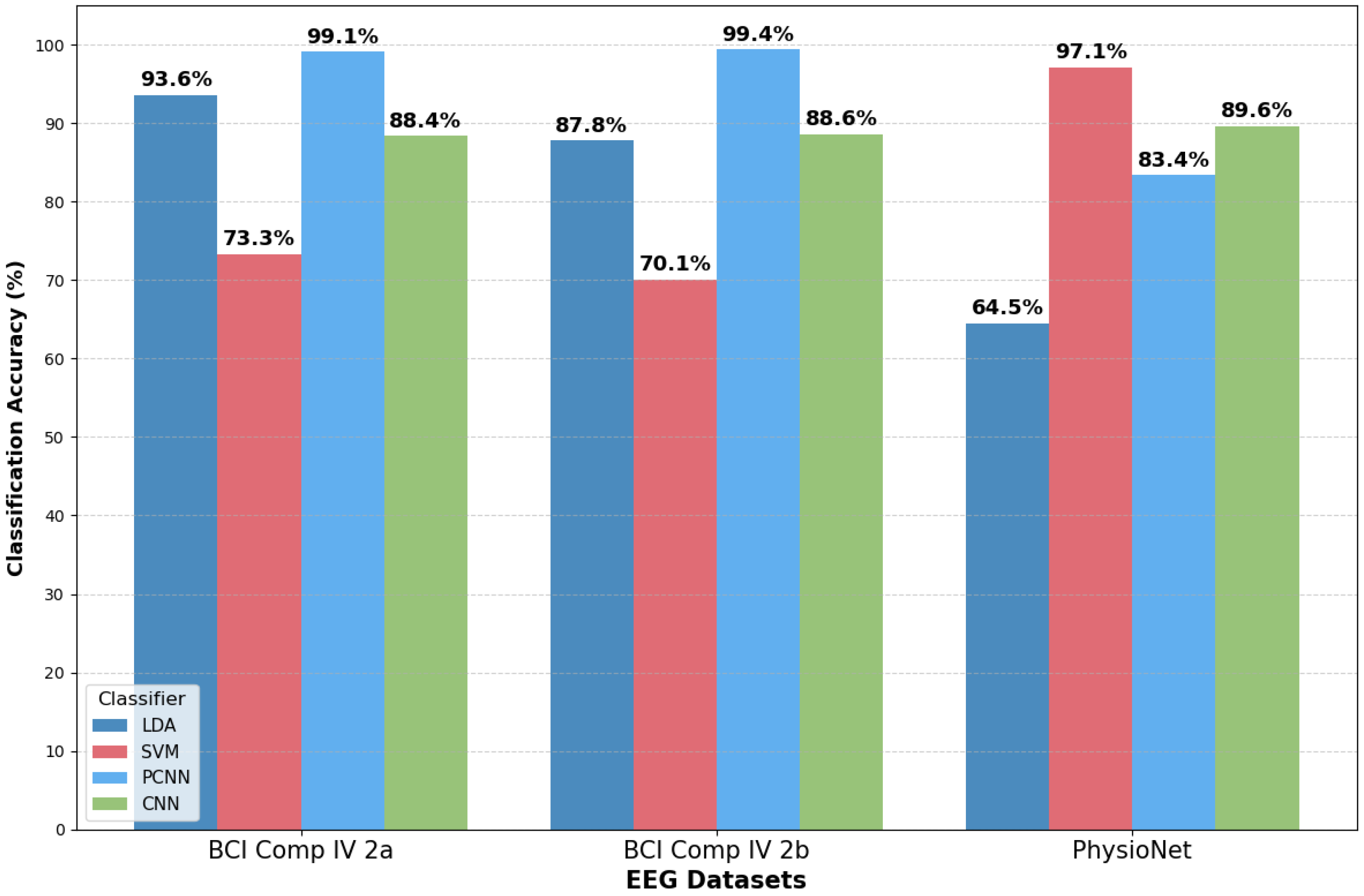
BCI Competition IV 2a is the most challenging among the three due to its four-class motor imagery paradigm recorded from 22 channels. Multi-class classification is more challenging because overlapping spatial–temporal patterns make it more complex to discriminate between left-hand, right-hand, foot, and tongue imagery. The results’ comparison is reflected in Figure 11, where advanced methods, such as PCNN, achieve a near-perfect performance of 99.1%, while simpler classifiers, like LDA, drop to 93.6%, and SVM struggles at 73.3%. The dataset therefore acts as a stress test for decomposition and feature extraction, where only models able to extract robust discriminative patterns across multiple classes maintain strong accuracy.
BCI Competition IV 2b simplifies the task to two classes and only three channels, focusing on left-hand vs. right-hand imagery. Reducing the number of channels lowers computational demands but also restricts spatial richness. As a result, accuracy patterns shift. PCNN demonstrates a slight improvement in the binary setting of BCI IV-2b with 99.4% accuracy due to clearer class separation between left- and right-hand imagery. LDA remains strong at 87.8% owing to a simpler class structure. In contrast, CNN shows only a marginal gain at 88.6%, compared to its previous performance, with a difference of only 0.2%, signaling that deep models struggle to utilize their hierarchical learning when limited to three channels. This indicates that reducing the number of classes can ease classification, but a loss of spatial richness limits the capacity of complex models to demonstrate their full potential. This balance highlights why IV 2b is less suitable for evaluating deep learning pipelines, even though classical methods remain competitive.
PhysioNet EEG Motor Movement/imagery introduces different challenges: a very large subject pool (109) and 64 channels, including both executed and imagined tasks. The increased inter-subject variability and noise make generalization far more difficult. This dataset emphasizes the challenge of generalization due to its extensive subject pool and significant inter-subject variability. In this context, CNNs perform well with an accuracy of 89.6%, demonstrating their adaptability to varied and noisy signals. However, the performance of PCNN sees a notable decrease in accuracy to about 83.4%, despite strong results in more controlled datasets. This suggests that PCNN may overfit to structured data. Interestingly, SVM achieves peak accuracy at about 97.1%, indicating its effectiveness in utilizing structured spectral features in heterogeneous environments. LDA drops drastically to 64.5%, highlighting its inadequacy in modeling the complex patterns present in a diverse population.
Overall, these datasets highlight how dataset characteristics directly influence high or low accuracy. Multi-class, high-channel datasets like IV 2a demand sophisticated feature extraction and decomposition. Binary, low-channel datasets like IV 2b allow even simpler methods to achieve strong results, but limit deep models, and large-scale, variable datasets like physioNet stress the ability to generalize across subjects, favoring classifiers tuned to variability.

Class-Based Performance (Two-Class vs. Four-Class)

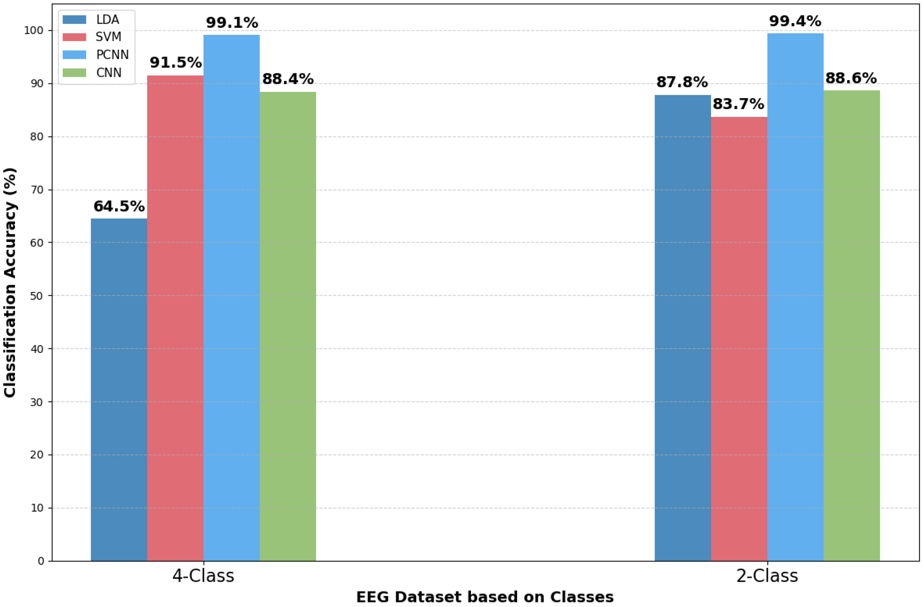
Two-class motor imagery tasks are inherently easier to model, because the neural signatures of left- and right-hand imagery tend to be more distinct and present less overlap across electrodes. As observed in Figure 12, the tight clustering of accuracy across methods highlights how binary paradigms provide clearer discriminative boundaries, making even simpler classifiers viable. The fact that PCNN edges ahead so sharply suggests that decomposition + learning hybrids can exploit that clarity to near-perfect separation. Similar observations are made by Zhu et al. [81], who showed that attention-fusion networks retain robustness across spatial resolution and individual variability in MI tasks.
When the problem expands to four classes, complexity increases: overlapping spectral patterns, shared cortical zones, and temporal dynamics make class separation more difficult. The wide spread in performance from 64.5% to 99.1% reveals that success in multi-class setups is highly contingent on the model capacity and feature extraction. Reviews of deep learning for MI-EEG classification, particularly one by Wang et al. [82], demonstrated that when tasks involve multiple classes, the performance sensitivity tends to increase.
The distinction between two-class and four-class classification tasks highlights a notable reduction in difficulty as well as an increase in variance across models. In Figure 11, the mean of the four-class accuracies is about 85.9% with much higher variability, demonstrating that a four-class classification not only lowers the baseline but also accuracy, but also emphasizes differences among methods. Ma et al. [83] highlighted in their study that there is a consistent decline in accuracy when transitioning from binary to multi-class classification frameworks.

3.3. Performance Evaluation Based on BCI Methods

Performance results’ analysis demonstrates that the selection of feature extraction and classification methods has a significant influence on the EEG-based motor imagery. Figure 13 and Figure 14 illustrate the performance analysis of the system when different methods are used.
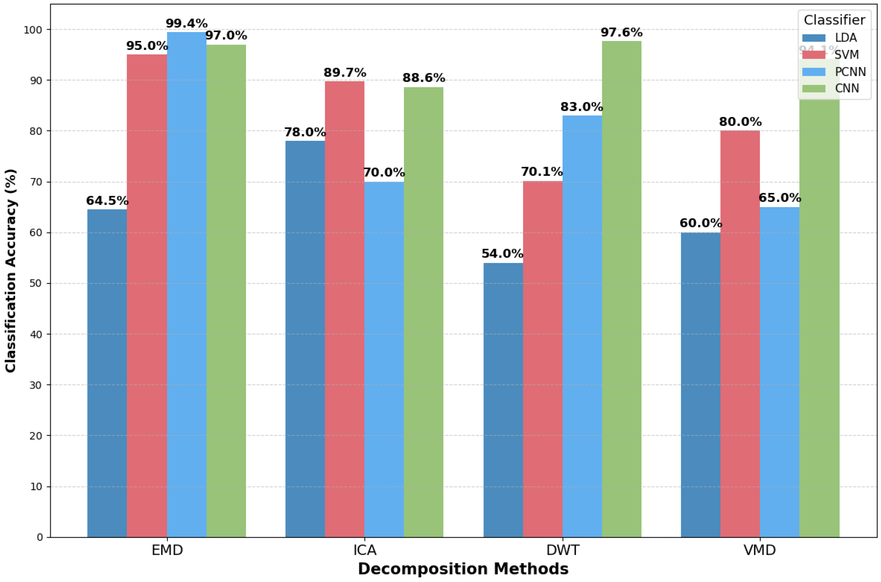
Figure 13 shows performance evaluation on different decomposition methods. At 99.39% accuracy, EMD surpasses other decomposition techniques, with PCNN obtaining the best accuracy. The strong CNN performance of 97.61% indicates that DWT is suitable for deep learning-based classification. ICA obtains moderate results, while SVM shows 89.7%. VMD performs well with CNN at 80% but not as well as EMD and DWT. EMD is very good at extracting discriminative features from EEG data for PCNN, indicating that it can maintain time–frequency features that are important for classification.
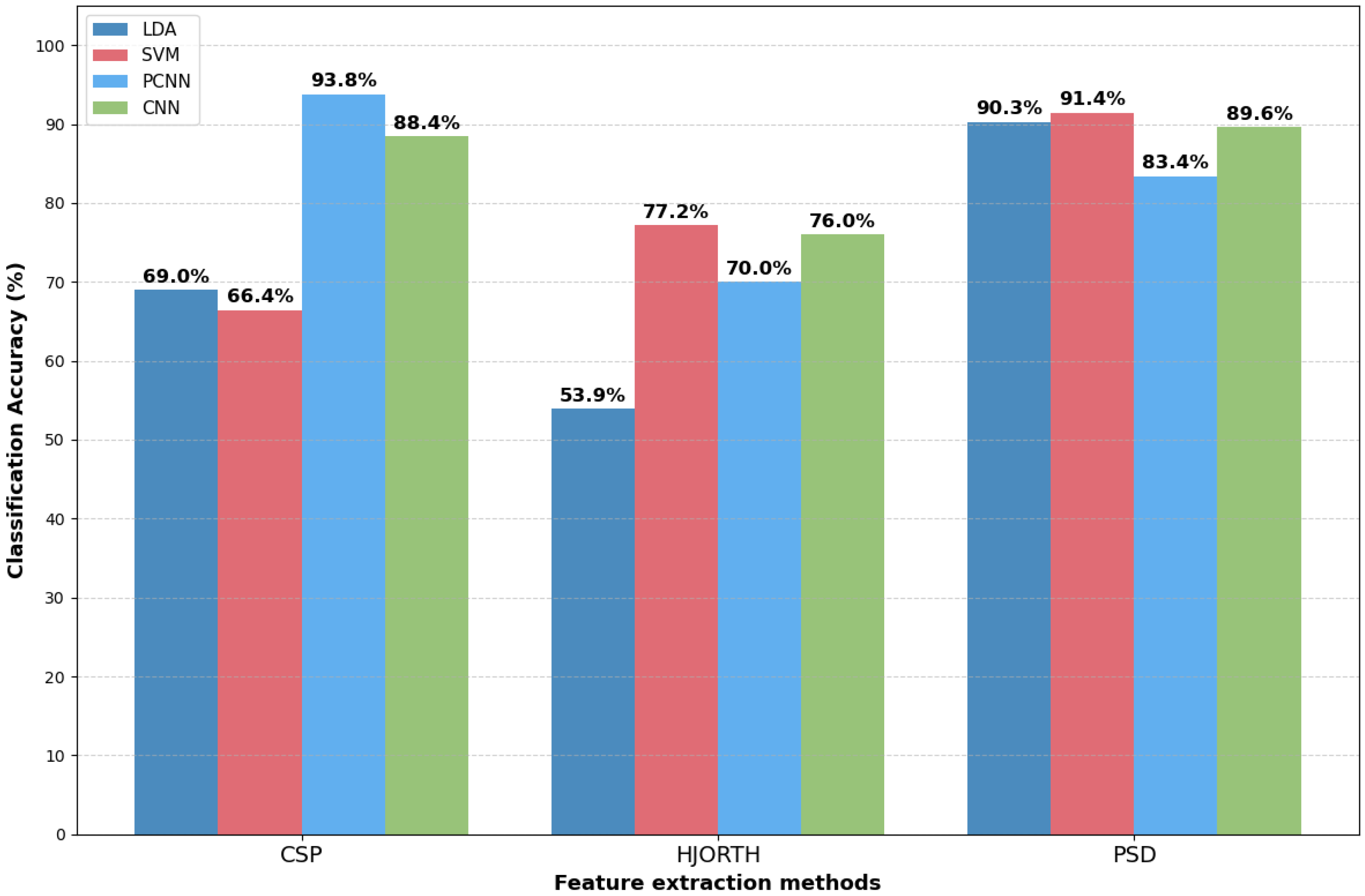
Figure 14 shows the impact of different feature extraction techniques on classification performance. PSD outperforms all three methods, but PCNN used with CSP yields the best performance at 93.8%. The properties of PSD and frequency are better for margin-based approaches, while PSD + SVM is better for spectral information. CSP + PCNN is best suited for spatial features.
Three dominant trends can be extracted from Table 4 and Figure 11, Figure 12, Figure 13 and Figure 14.
Spectral- and Temporal-Domain Methods: The EMD and PCNN methods achieve the highest classification accuracy among all other paradigms, with 99% accuracy in both two-class and four-class paradigms. The advantage inherent in this approach is that EMD can adaptively decompose nonstationary EEG signals into IMFs, which retain the important nonlinear oscillatory characteristics associated with MI. When a PCNN processes such IMFs, the network can pick up on complex temporal as well as spectral features, which explains the high accuracy [53]. Use of band power and Hjorth parameters with LDA also provided decent performance of about 93% accuracy in two-class experiments. Those features incorporate the frequency as well as the temporal characteristics of the EEG signals and require far less computational intensity than deep learning methods. These methods are especially desirable for real-time use. On the other hand, when looking at Butterworth filtering with sliding windows, together with PCNN, it also shows remarkably high efficiency for binary-class tasks of about 99.7% but a steep degradation for four-class paradigms (83%) [84]. This indicates that, despite the fact that temporal filtering as well as segmentation can be adequate for smaller tasks, their ability to separate complex multi-class patterns is not.
Spatial-Domain Methods: CSP/SVM and CSP/LDA methods offer average accuracy, between 64 and 73% for two-class tasks, but underperform for four-class tasks. The best performance by CSP occurs when motor imagery patterns show obvious spatial separations between the electrodes. However, overlapping activation across cortices in multi-class cases reduces its discriminative power [85]. Furthermore, the CSP-driven methods are highly susceptible to inter-subject variability and EEG noise, which contributes to their lower robustness relative to deep learning methods. These findings suggest that spatial features do preserve useful information, but that spatial features by themselves are insufficient for processing noisy or complex EEG data.
Deep learning methods: Pure CNN models demonstrate strong performance in classifying both two-class and four-class paradigms, achieving accuracies in the high 80s. Specifically, when applied to the physioNet dataset, CNNs reach about 89% accuracy for executed tasks and approximately 87% for imagined tasks, indicating their effectiveness in handling both real and imagined motor imagery. A key advantage of CNNs is their capacity to learn temporal and spatial hierarchies directly from raw or minimally processed EEG signals, which reduces their reliance on handcrafted features. Nevertheless, studies reveal that hybrid models, such as EMD + PCNN, statistically outperform pure CNNs in performance metrics [56].
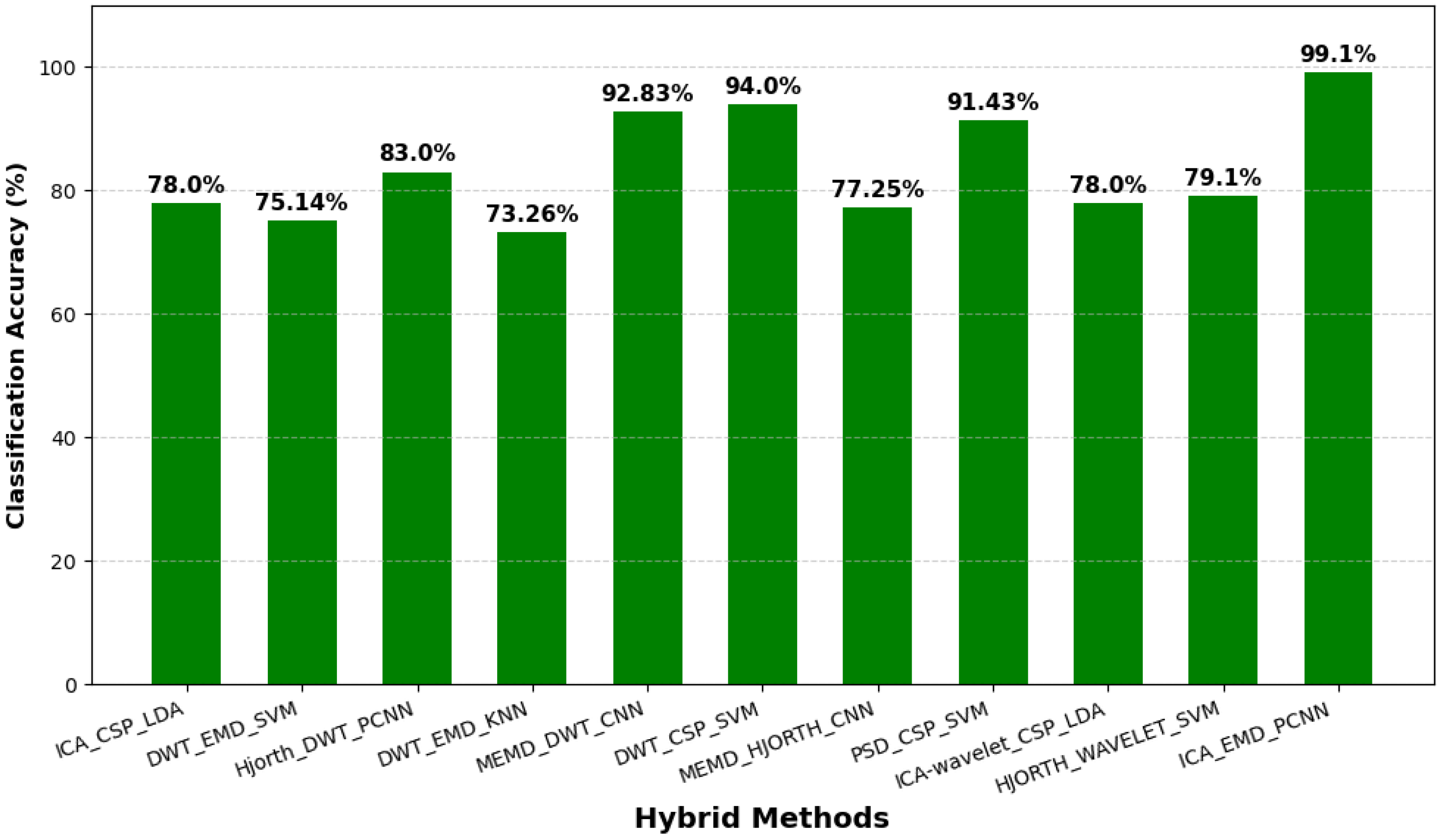
Figure 15 illustrates how combining multiple decomposition or feature extraction techniques can result in notable performance improvements. The choice of classifier is essential since the excellent accuracy of ICA_EMD_PCNN indicates that EMD captures nonlinear and non-stationary components, whereas ICA separates independent EEG sources. This emphasizes the importance of hybrid pipeline design that leverages the strengths of multiple signal processing and classification strategies for achieving optimal EEG decoding performance.
The analysis of deep learning versus hybrid approaches indicates a distinct correlation between architectural design and classification accuracy of motor imagery EEG. Pure architectures, such as CNNs and LSTMs, achieve moderate levels of accuracy, typically ranging from 82% to 88%, demonstrating their limitations when used in isolation [74,86]. CNNs are well-suited for extracting spatial information from EEG electrode maps, but do not fully capture the temporal dynamics of brain activity. In contrast, LSTMs are capable of modeling time dependencies but lack spatial discrimination. When these are combined, their complementary strengths become evident. A CNN-LSTM hybrid, for example, constantly improves classification results, reaching around 96% on benchmark datasets such as PysioNet. This improvement arises because CNNs extract spatial structure while LSTMs account for the sequential nature of EEG signals. More advanced designs, such as CNN-GRU hybrid, push performance further, achieving above 99% in some studies [87,88,89]. These gains are often supported by strong data augmentation strategies and carefully curated datasets, which means that while accuracy is very high in controlled conditions, real-world robustness may still be an open question. While hybrid methods achieve higher classification accuracy, the added complexity of combining multiple transformations may increase the risk of sample distortion, such as redundancy or loss of fine signal characteristics. In contrast, single methods, although less accurate, are less prone to altering the new EEG signal structure.
Performance in BCI research demonstrates significant challenges when dealing with complex datasets, notably in BCI competition IV-2a, which involves discerning four motor imagery tasks from multiple participants. Even with the advanced hybrid feature extraction and classification techniques, accuracy levels tend to fall to approximately 83%. This notable drop in performance is primarily due to the difficulties in differentiating overlapping cortical activations and accommodating inter-subject variability. Despite these challenges, hybrid feature extraction and classification techniques have demonstrated robust performance, frequently outperforming single models. Recent research has also shed light on the effectiveness of combining efficient classifiers with specially designed features to enhance performance. Significantly, the MiniRocket approach, being less computationally expensive, has achieved accuracies of up to 99% [90,91,92]. Its performance is on par with heavy deep hybrid models, highlighting the value of properly designed features for extraction as needed for resource-limited real-time applications. Optimal prospects for the improvement of BCI performance using innovative combination strategies for both classifiers and features now seem possible. Hybrid models emerge as the most consistent means to achieve high accuracy, as they integrate both spatial and temporal features crucial for decoding EEG signals. Nevertheless, their effectiveness heavily relies on the dataset used, the number of classes, and their ability to generalize across different subjects. Lightweight methods rooted in efficient feature engineering remain a viable option, indicating that no singular best method exists; rather, a balance must be struck between accuracy, robustness, and computational feasibility.
The results in Figure 16 show precision, recall, and F1 score metrics for each signal processing pipeline, which complement classification accuracy and provide insights into the balance of true positive detections and false classifications, the key factors in determining the reliability of a system for real-time BCI applications. Precision indicates the model’s ability to correctly identify true target events without false alarms, recall measures its sensitivity in detecting all relevant instances, and F1 score provides a balanced representation of both.
The results indicate that the hybrid pipelines that integrate EMD with deep or spatial feature-learning methods (EMD + PCNN and EMD + CSP) perform better than traditional machine learning models, with the best and most balanced metrics. This reflects a balanced model that generalizes well across subjects, demonstrating higher adaptability to individual subject variability and robustness against signal noise. CSP + SVM and CSP + PSD + CNN showed lower scores, due to their limited sensitivity to the non-stationary nature of EEG signals. These results indicate that adaptive decomposition can better extract discriminative time–frequency spatial features, and deep learning can improve pattern recognition.
For real-time applications of BCI models, computational complexity has become a key metric for assessing the practicality of the models. While traditional feature methods, such as CSP and PSD, are computationally lightweight and suitable for online processing, they often lack representation capability for non-stationary EEG signals. In contrast, decomposition-based methods such as EMD, VMD, and EWT are typically more computationally demanding and have time complexity, which can lead to increased processing latency in real-time applications.
However, the computational burden (especially during training) has increased with deep learning architectures such as CNNs, RNNs, and hybrid models, due to the large number of parameters and multi-layer operations. These have shown better performance in capturing the spatial–temporal dependencies in EEG signals; however, recent efforts have aimed at optimizing this trade-off by using lightweight architectures [93] (e.g., MobileNet, EEGNet) and model compression techniques that reduce the number of parameters while maintaining accuracy. Thus, although deep models perform better, they cannot be deployed in real-time or wearable BCI systems due to computational cost and latency.

4. Discussion

Traditional FIR and IIR filters remain indispensable for basic preprocessing. They reduce line interference and confine the EEG to mu and beta, where motor imagery features reside. These bands are central to motor imagery studies, which explains why such filters remain a standard first step. The drawbacks, however, lie in their rigidity: EEG signals are highly nonstationary, and fixed filters cannot adapt to the rapid, transient artifacts and overlapping oscillations that often appear in real recordings. BCI relies on EEG signals to interpret and predict user actions without physical movement. These are sensitive signals that are susceptible to distortion from physiological artifacts and noise. Cleaning and improving EEG data is essential for producing precise predictions. However, there is a chance that excessive data cleaning will result in the loss of crucial signal elements that express the user’s intent. ICA has long been the gold standard for artifact removal, especially for eye blinks and muscle activity. Yet it suffers from variability across subjects and instability when the signal-to-noise ratio is poor. CNNs and PCNNs bypass these issues by directly learning spatial–temporal representation from raw or minimally processed EEG. This explains their consistently higher classification accuracies (95–99%) compared with ICA-dependent pipelines (70–80%). However, CNNs are heavily data-dependent and risk overfitting when the training sets are small.
Hybrid approaches that integrate decomposition methods such as EMD with deep neural architectures demonstrate superior performance compared to single models, as they leverage the complementary strengths of both techniques. Decomposition methods maintain oscillatory details, while CNNs capture complex nonlinear relationships. This synergy enables EMD-PCNN pipelines to achieve near-optimal performance in both two-class and four-class paradigms [94]. The findings indicate that reliance on single methods increases the likelihood of sample damage or reduced performance, whereas hybrid models mitigate this risk by merging diverse feature perspectives. However, using deep and hybrid approaches presents challenges, including high computational demands and potential latency issues in real-time BCI applications. While autoencoders and GANs can improve denoising and data augmentation processes, they introduce complications such as reconstruction loss and training instability [95]. Furthermore, emerging techniques like transformers hold promise for capturing long-range dependencies in EEG data, yet their application in motor imagery tasks is still limited, necessitating significantly larger datasets for effective implementation. The findings illustrate a notable evolution in processing methods, with classical techniques still pertinent for lightweight and real-time applications but increasingly being eclipsed by deep learning and hybrid approaches that deliver enhanced accuracy and robustness. CNNs and PCNNs are highlighted as effective, yet their practical application requires balancing accuracy with computational efficiency. Nonetheless, ongoing research is needed to address the surrounding generalization and the real-time adaptability of these systems. Future research should also explore the integration of newer architectures, including GAN-based augmentation, to improve the scalability and resilience of BCIs. Since brain signals differ from subject to subject and session to session, no single method works perfectly across all EEG datasets or users. In order to be effective, preprocessing frequently has to be adaptive, modifying parameters according to the signal patterns of each user and the conditions of real-time recording. Accurate BCI performance requires careful preprocessing. Strategies that strike a balance between eliminating noise and preserving delicate brain inputs yield the most effective outcomes. Research is shifting towards more clever, flexible techniques that can maintain this balance, increasing the dependability of BCI systems in both controlled lab settings and real-world assistive environments. Table 5 highlights the advantages and limitations of BCI methods, providing a clear overview of how researchers can combine well-suited methods for optimal and sustainable BCI performance.

5. Conclusions

This paper examined the performance of feature extraction and classification methods in EEG-based brain–computer interface (BCI) systems and highlights the importance of BCI pipelines and how different methods and dataset characteristics play a huge role in the performance of the system. The effectiveness of component integration and tailoring to the specific BCI task at hand directly determines high accuracy and performance. It presented a comprehensive, detailed literature review of commonly utilized EEG signal filtering techniques. The review focused on the preprocessing stage of EEG-based BCIs, focusing on the removal of noise and artifacts through filtering and decomposition techniques. It also examined the impact of feature extraction on system performance, looking at different classification methods from ML and DL to hybrid methods. It evaluated the significance of advanced preprocessing pipelines focusing on ICA, EMD, Hjorth parameters, CSP, PSD, and wavelet-based methods. This was achieved using classifiers to evaluate the performance of each dataset, class, decomposition, and feature extraction technique. Pre-classification processing of EEG data has a significant effect on performance. CNNs and PCNNs directly learn spatial–temporal representation from raw or minimally processed EEG. This explains their consistently higher classification accuracies (95–99%) compared with ICA-dependent pipelines (70–80%). Single methods increase the likelihood of sample damage or reduced performance, whereas hybrid models mitigate this risk by merging diverse feature perspectives. Future developments are expected to highlight energy-efficient algorithms, parallel computing, and edge computing, which will allow for fast, low-power BCI systems without compromising signal fidelity. Recent developments in BCI research highlight the need for systems that are tailored to individual users, minimize calibration times, and ensure low latency in real-world operations. Integrating adaptive learning and online feedback mechanisms could allow the pipeline to adapt to user variability, cognitive load, and session changes. Such approaches would move systems from pure algorithmic optimization to a personalized, user-driven BCI framework, which would improve their usability and long-term use in smart assistive environment. The reviewed methods yielded remarkable performances for within-subject classification, highlighting the significance of artifact rejection towards higher BCI performances. However, IDRs significantly vary from subject to subject due to immense variations in EEG neural dynamics across individual subjects. Hence, a more robust domain adaptation algorithm based on domain selection will be explored in future work.

Author Contributions

Conceptualization, B.M. and R.C.M.; methodology, B.M. and R.C.M.; validation, B.M. and R.C.M.; formal analysis, B.M.; investigation, B.M.; writing—original draft preparation, B.M.; writing—review and editing, R.C.M. and P.K.; visualization, B.M.; supervision, R.C.M. and P.K.; project administration, R.C.M. and P.K.; funding acquisition, R.C.M. and P.K. All authors have read and agreed to the published version of the manuscript.

Funding

This research was funded by the National Research Foundation of South Africa (Grant Number: PMDS240702237542).

Institutional Review Board Statement

Not applicable.

Informed Consent Statement

Not applicable.

Data Availability Statement

The datasets used are publicly available online and from the corresponding author upon reasonable request.

Conflicts of Interest

The authors declare no conflicts of interest.

Abbreviations

The following abbreviations are used in this manuscript:
EEGElectroencephalogram
BCIBrain–Computer Interface
PCNNParallel Convolutional Neural Network
LDALinear Discriminant Analysis
CNNConvolutional Neural Network
EMDEmpirical Mode Decomposition
ICA Independent Component Analysis
PSDPower Spectral Density
CSPCommon Spatial Pattern
AMICAAdaptive Mixture Independent Component Analysis
DWTDiscrete Wavelet Transform
DNNDeep Neural Networks
NNNeural Networks
IDRIntention Detection Rate
DLDeep Learning
MLMachine Learning

References

  1. Peksa, J.; Mamchur, D. State-of-the-art on brain-computer interface technology. Sensors 2023, 23, 6001. [Google Scholar] [CrossRef] [PubMed]
  2. Brophy, E.; Redmond, P.; Fleury, A.; De Vos, M.; Boylan, G.; Ward, T. Denoising EEG signals for real-world BCI applications using GANs. Front. Neuroergonomics 2022, 2, 805573. [Google Scholar] [CrossRef] [PubMed]
  3. Vavoulis, A.; Figueiredo, P.; Vourvopoulos, A. A review of online classification performance in motor imagery-based brain–computer interfaces for stroke neurorehabilitation. Signals 2023, 4, 73–86. [Google Scholar] [CrossRef]
  4. Lotte, F.; Bougrain, L.; Cichocki, A.; Clerc, M.; Congedo, M.; Rakotomamonjy, A.; Yger, F. A review of classification algorithms for EEG-based brain–computer interfaces: A 10 year update. J. Neural Eng. 2018, 15, 031005. [Google Scholar] [CrossRef]
  5. Saha, S.; Mamun, K.A.; Ahmed, K.; Mostafa, R.; Naik, G.R.; Darvishi, S.; Khandoker, A.H.; Baumert, M. Progress in brain computer interface: Challenges and opportunities. Front. Syst. Neurosci. 2021, 15, 578875. [Google Scholar] [CrossRef]
  6. Nasim, S.F.; Fatimah, S.; Amin, A. Artificial intelligence in motor imagery-based bci systems: A narrative. Asian J. Med. Technol. 2022, 2, 55–64. [Google Scholar] [CrossRef]
  7. Novičić, M.; Djordjević, O.; Miler-Jerković, V.; Konstantinović, L.; Savić, A.M. Improving the Performance of Electrotactile Brain–Computer Interface Using Machine Learning Methods on Multi-Channel Features of Somatosensory Event-Related Potentials. Sensors 2024, 24, 8048. [Google Scholar] [CrossRef]
  8. Xu, H.; Hassan, S.A.; Haider, W.; Sun, Y.; Yu, X. A Frequency-Shifting Variational Mode Decomposition-Based Approach to MI-EEG Signal Classification for BCIs. Sensors 2025, 25, 2134. [Google Scholar] [CrossRef]
  9. Sakib, M.; Md Shafayet, H.; Muhammad EH, C. MLMRS-Net Electroencephalography (EEG) motion artifacts removal using a multi-layer multi-resolution spatially pooled 1D signal reconstruction network. Neural Comput. Appl. 2023, 35, 8371–8388. [Google Scholar]
  10. An, Y.; Lam, H.K.; Ling, S.H. Multi-classification for EEG motor imagery signals using data evaluation-based auto-selected regularized FBCSP and convolutional neural network. Neural Comput. Appl. 2023, 35, 12001–12027. [Google Scholar] [CrossRef]
  11. Huang, X.; Xu, Y.; Hua, J.; Yi, W.; Yin, H.; Hu, R.; Wang, S. A review on signal processing approaches to reduce calibration time in EEG-based brain–computer interface. Front. Neurosci. 2021, 15, 733546. [Google Scholar] [CrossRef]
  12. Wang, Z.; Juhasz, Z. GPU Implementation of the Improved CEEMDAN Algorithm for Fast and Efficient EEG Time–Frequency Analysis. Sensors 2023, 23, 8654. [Google Scholar] [CrossRef] [PubMed]
  13. Tong, J.; Xing, Z.; Wei, X.; Yue, C.; Dong, E.; Du, S.; Sun, Z.; Solé-Casals, J.; Caiafa, C.F. Towards improving motor imagery brain–computer interface using multimodal speech imagery. J. Med. Biol. Eng. 2023, 43, 216–226. [Google Scholar] [CrossRef]
  14. Sheng, H.; Wu, Q.; Chi, R.; Guo, Z. Time-Frequency Double-Dimensional Multi-Scale CNN with Attention Mechanism for Motor Imagery EEG Signal Classification. Appl. Comput. Eng. 2025, 132, 284–292. [Google Scholar] [CrossRef]
  15. Mohamed, A.F.; Jusas, V. Advancing Fractal Dimension Techniques to Enhance Motor Imagery Tasks Using EEG for Brain–Computer Interface Applications. Appl. Sci. 2025, 15, 6021. [Google Scholar] [CrossRef]
  16. Huang, W.; Yan, G.; Chang, W.; Zhang, Y.; Yuan, Y. EEG-based classification combining Bayesian convolutional neural networks with recurrence plot for motor movement/imagery. Pattern Recognit. 2023, 144, 109838. [Google Scholar] [CrossRef]
  17. Gao, Z.; Dang, W.; Wang, X.; Hong, X.; Hou, L.; Ma, K.; Perc, M. Complex networks and deep learning for EEG signal analysis. Cogn. Neurodyn. 2021, 15, 369–388. [Google Scholar] [CrossRef]
  18. Agrawal, R.; Dhule, C.; Shukla, G.; Singh, S.; Agrawal, U.; Alsubaie, N.; Alqahtani, M.S.; Abbas, M.; Soufiene, B.O. Design of EEG based thought identification system using EMD & deep neural network. Sci. Rep. 2024, 14, 26621. [Google Scholar] [CrossRef]
  19. Hu, W.; Geng, X.; Yue, M.; Wang, L.; Zhang, X. Feature extraction of motor imagery EEG signals based on PSD CSP fusion. In Intelligent Computing Technology and Automation; IOS Press: Amsterdam, The Netherlands, 2024; pp. 66–72. [Google Scholar]
  20. Antony, M.J.; Sankaralingam, B.P.; Mahendran, R.K.; Gardezi, A.A.; Shafiq, M.; Choi, J.-G.; Hamam, H. Classification of EEG using adaptive SVM classifier with CSP and online recursive independent component analysis. Sensors 2022, 22, 7596. [Google Scholar] [CrossRef]
  21. Mehla, V.K.; Singhal, A.; Singh, P. EMD-based discrimination of mental arithmetic tasks from EEG signals. In Proceedings of the 2020 IEEE 17th India Council International Conference (INDICON), New Delhi, India, 11–13 December 2020; pp. 1–4. [Google Scholar]
  22. Hu, H.; Pu, Z.; Li, H.; Liu, Z.; Wang, P. Learning optimal time-frequency-spatial features by the cissa-csp method for motor imagery eeg classification. Sensors 2022, 22, 8526. [Google Scholar] [CrossRef]
  23. Saghab Torbati, M.; Zandbagleh, A.; Daliri, M.R.; Ahmadi, A.; Rostami, R.; Kazemi, R. Explainable AI for Bipolar Disorder Diagnosis Using Hjorth Parameters. Diagnostics 2025, 15, 316. [Google Scholar] [CrossRef]
  24. Miao, M.; Hu, W.; Yin, H.; Zhang, K. Spatial-Frequency Feature Learning and Classification of Motor Imagery EEG Based on Deep Convolution Neural Network. Comput. Math. Methods Med. 2020, 2020, 1981728. [Google Scholar] [CrossRef]
  25. Xu, J.; Zheng, H.; Wang, J.; Li, D.; Fang, X. Recognition of EEG signal motor imagery intention based on deep multi-view feature learning. Sensors 2020, 20, 3496. [Google Scholar] [CrossRef] [PubMed]
  26. Gwon, D.; Won, K.; Song, M.; Nam, C.S.; Jun, S.C.; Ahn, M. Review of public motor imagery and execution datasets in brain-computer interfaces. Front. Hum. Neurosci. 2023, 17, 1134869. [Google Scholar] [PubMed]
  27. KC, S. Parallel convolutional neural network and empirical mode decomposition for high accuracy in motor imagery EEG signal classification. PLoS ONE 2025, 20, e0311942. [Google Scholar]
  28. Gaur, P.; Pachori, R.B.; Wang, H.; Prasad, G. An empirical mode decomposition based filtering method for classification of motor-imagery EEG signals for enhancing brain-computer interface. In Proceedings of the 2015 International Joint Conference on Neural Networks (IJCNN), Killarney, UK, 12–17 July 2015; pp. 1–7. [Google Scholar]
  29. Zhang, C.; Kim, Y.-K.; Eskandarian, A. EEG-inception: An accurate and robust end-to-end neural network for EEG-based motor imagery classification. J. Neural Eng. 2021, 18, 046014. [Google Scholar] [CrossRef] [PubMed]
  30. Wang, X.; Dai, X.; Liu, Y.; Chen, X.; Hu, Q.; Hu, R.; Li, M. Motor imagery electroencephalogram classification algorithm based on joint features in the spatial and frequency domains and instance transfer. Front. Hum. Neurosci. 2023, 17, 1175399. [Google Scholar] [CrossRef]
  31. Chowdhury, R.R.; Muhammad, Y.; Adeel, U. Enhancing cross-subject motor imagery classification in EEG-based brain–computer interfaces by using multi-branch CNN. Sensors 2023, 23, 7908. [Google Scholar] [CrossRef]
  32. Lv, R.; Chang, W.; Yan, G.; Sadiq, M.T.; Nie, W.; Zheng, L. Enhanced classification of motor imagery EEG signals using spatio-temporal representations. Inf. Sci. 2025, 714, 122221. [Google Scholar] [CrossRef]
  33. Alomari, M.H.; Samaha, A.; AlKamha, K. Automated classification of L/R hand movement EEG signals using advanced feature extraction and machine learning. arXiv 2013, arXiv:1312.2877. [Google Scholar] [CrossRef]
  34. Tibrewal, N.; Leeuwis, N.; Alimardani, M. Classification of motor imagery EEG using deep learning increases performance in inefficient BCI users. PLoS ONE 2022, 17, e0268880. [Google Scholar] [CrossRef]
  35. Hong, S.; Baek, H.J. Drowsiness detection based on intelligent systems with nonlinear features for optimal placement of encephalogram electrodes on the cerebral area. Sensors 2021, 21, 1255. [Google Scholar] [CrossRef] [PubMed]
  36. Kawala-Sterniuk, A.; Browarska, N.; Al-Bakri, A.; Pelc, M.; Zygarlicki, J.; Sidikova, M.; Martinek, R.; Gorzelanczyk, E.J. Summary of over fifty years with brain-computer interfaces—A review. Brain Sci. 2021, 11, 43. [Google Scholar] [CrossRef] [PubMed]
  37. Cao, Z. A review of artificial intelligence for EEG-based brain− computer interfaces and applications. Brain Sci. Adv. 2020, 6, 162–170. [Google Scholar] [CrossRef]
  38. Singh, A.K.; Krishnan, S. Trends in EEG signal feature extraction applications. Front. Artif. Intell. 2023, 5, 1072801. [Google Scholar] [CrossRef]
  39. Rashid, M.; Sulaiman, N.; PP Abdul Majeed, A.; Musa, R.M.; Ab Nasir, A.F.; Bari, B.S.; Khatun, S. Current status, challenges, and possible solutions of EEG-based brain-computer interface: A comprehensive review. Front. Neurorobot. 2020, 14, 25. [Google Scholar] [CrossRef]
  40. Chaddad, A.; Wu, Y.; Kateb, R.; Bouridane, A. Electroencephalography signal processing: A comprehensive review and analysis of methods and techniques. Sensors 2023, 23, 6434. [Google Scholar] [CrossRef]
  41. Sun, C.; Mou, C. Survey on the research direction of EEG-based signal processing. Front. Neurosci. 2023, 17, 1203059. [Google Scholar] [CrossRef]
  42. Karpiel, I.; Kurasz, Z.; Kurasz, R.; Duch, K. The influence of filters on EEG-ERP testing: Analysis of motor cortex in healthy subjects. Sensors 2021, 21, 7711. [Google Scholar] [CrossRef]
  43. Vasei, T.; Saber, M.A.; Nahvy, A.; Navabi, Z. An Efficient RTL Design for a Wearable Brain–Computer Interface. IET Comput. Digit. Tech. 2024, 2024, 5596468. [Google Scholar] [CrossRef]
  44. An, X.; K Stylios, G. Comparison of motion artefact reduction methods and the implementation of adaptive motion artefact reduction in wearable electrocardiogram monitoring. Sensors 2020, 20, 1468. [Google Scholar] [CrossRef]
  45. Shakeel, A.; Onojima, T.; Tanaka, T.; Kitajo, K. Real-time implementation of EEG oscillatory phase-informed visual stimulation using a least mean square-based AR model. J. Pers. Med. 2021, 11, 38. [Google Scholar] [CrossRef] [PubMed]
  46. Alturki, F.A.; AlSharabi, K.; Abdurraqeeb, A.M.; Aljalal, M. EEG signal analysis for diagnosing neurological disorders using discrete wavelet transform and intelligent techniques. Sensors 2020, 20, 2505. [Google Scholar] [CrossRef] [PubMed]
  47. Klug, M.; Berg, T.; Gramann, K. Optimizing EEG ICA decomposition with data cleaning in stationary and mobile experiments. Sci. Rep. 2024, 14, 14119. [Google Scholar] [CrossRef] [PubMed]
  48. Ouyang, G.; Li, Y. Protocol for semi-automatic EEG preprocessing incorporating independent component analysis and principal component analysis. STAR Protoc. 2025, 6, 103682. [Google Scholar] [CrossRef]
  49. Mäkelä, S.; Kujala, J.; Salmelin, R. Removing ocular artifacts from magnetoencephalographic data on naturalistic reading of continuous texts. Front. Neurosci. 2022, 16, 974162. [Google Scholar] [CrossRef]
  50. Ferrari, A.; Filippin, L.; Buiatti, M.; Parise, E. WTools: A MATLAB-based toolbox for time-frequency analysis. bioRxiv 2024. [Google Scholar]
  51. Raveendran, S.; Kenchaiah, R.; Kumar, S.; Sahoo, J.; Farsana, M.; Chowdary Mundlamuri, R.; Bansal, S.; Binu, V.; Ramakrishnan, A.; Ramakrishnan, S. Variational mode decomposition-based EEG analysis for the classification of disorders of consciousness. Front. Neurosci. 2024, 18, 1340528. [Google Scholar] [CrossRef]
  52. Hu, L.; Zhao, K.; Zhou, X.; Ling, B.W.-K.; Liao, G. Empirical mode decomposition based multi-modal activity recognition. Sensors 2020, 20, 6055. [Google Scholar] [CrossRef]
  53. Jaipriya, D.; Sriharipriya, K. A comparative analysis of masking empirical mode decomposition and a neural network with feed-forward and back propagation along with masking empirical mode decomposition to improve the classification performance for a reliable brain-computer interface. Front. Comput. Neurosci. 2022, 16, 1010770. [Google Scholar] [CrossRef]
  54. Fang, Y.; Hou, J.; Liu, X.; Sun, Y.; Wang, H.; Li, J. Hybrid MVMD-ICA Framework for EOG Artifacts Removal from Few-Channel EEG Signals. In Proceedings of the 2025 6th International Conference on Bio-engineering for Smart Technologies (BioSMART), Paris, France, 14–16 May 2025; pp. 1–4. [Google Scholar]
  55. Hu, Q.; Li, M.; Li, Y. Single-channel EEG signal extraction based on DWT, CEEMDAN, and ICA method. Front. Hum. Neurosci. 2022, 16, 1010760. [Google Scholar] [CrossRef]
  56. Mwata-Velu, T.; Navarro Rodríguez, A.; Mfuni-Tshimanga, Y.; Mavuela-Maniansa, R.; Martínez Castro, J.A.; Ruiz-Pinales, J.; Avina-Cervantes, J.G. EEG-BCI Features Discrimination between Executed and Imagined Movements Based on FastICA, Hjorth Parameters, and SVM. Mathematics 2023, 11, 4409. [Google Scholar] [CrossRef]
  57. Alawee, W.H.; Basem, A.; Al-Haddad, L.A. Advancing biomedical engineering: Leveraging Hjorth features for electroencephalography signal analysis. J. Electr. Bioimpedance 2023, 14, 66. [Google Scholar] [CrossRef] [PubMed]
  58. Aggarwal, S.; Chugh, N. Signal processing techniques for motor imagery brain computer interface: A review. Array 2019, 1, 100003. [Google Scholar] [CrossRef]
  59. Ye, J. Challenges and Future Development of Neural Signal Decoding and Brain-Computer Interface Technology. J. Med. Life Sci. 2025, 1, 54–60. [Google Scholar]
  60. Suárez, M.; Torres, A.M.; Blasco-Segura, P.; Mateo, J. Application of the Random Forest Algorithm for Accurate Bipolar Disorder Classification. Life 2025, 15, 394. [Google Scholar] [CrossRef]
  61. Wu, S.; Bhadra, K.; Giraud, A.-L.; Marchesotti, S. Adaptive LDA classifier enhances real-time control of an EEG brain–computer interface for decoding imagined syllables. Brain Sci. 2024, 14, 196. [Google Scholar] [CrossRef]
  62. Abdulkareem, H.A.; Al-Faiz, M.Z. Offline linear discriminant analysis classfication of two class eeg signals. Iraqi J. Inf. Commun. Technol. 2019, 2, 1–10. [Google Scholar] [CrossRef]
  63. Li, X.; Chen, X.; Yan, Y.; Wei, W.; Wang, Z.J. Classification of EEG signals using a multiple kernel learning support vector machine. Sensors 2014, 14, 12784–12802. [Google Scholar] [CrossRef]
  64. Jun, Z. The development and application of support vector machine. J. Phys. Conf. Ser. 2021, 1748, 052006. [Google Scholar] [CrossRef]
  65. Aydin, S.; Melek, M.; Gökrem, L. A Safe and Efficient Brain–Computer Interface Using Moving Object Trajectories and LED-Controlled Activation. Micromachines 2025, 16, 340. [Google Scholar] [CrossRef]
  66. Kamhi, S.; Zhang, S.; Ait Amou, M.; Mouhafid, M.; Javaid, I.; Ahmad, I.S.; Abd El Kader, I.; Kulsum, U. Multi-classification of motor imagery EEG signals using Bayesian optimization-based average ensemble approach. Appl. Sci. 2022, 12, 5807. [Google Scholar] [CrossRef]
  67. Antoniou, E.; Bozios, P.; Christou, V.; Tzimourta, K.D.; Kalafatakis, K.; G Tsipouras, M.; Giannakeas, N.; Tzallas, A.T. EEG-based eye movement recognition using brain–computer interface and random forests. Sensors 2021, 21, 2339. [Google Scholar] [CrossRef] [PubMed]
  68. Hossain, K.M.; Islam, M.A.; Hossain, S.; Nijholt, A.; Ahad, M.A.R. Status of deep learning for EEG-based brain–computer interface applications. Front. Comput. Neurosci. 2023, 16, 1006763. [Google Scholar] [CrossRef] [PubMed]
  69. Rakhmatulin, I.; Dao, M.-S.; Nassibi, A.; Mandic, D. Exploring convolutional neural network architectures for EEG feature extraction. Sensors 2024, 24, 877. [Google Scholar] [CrossRef] [PubMed]
  70. Lun, X.; Yu, Z.; Chen, T.; Wang, F.; Hou, Y. A simplified CNN classification method for MI-EEG via the electrode pairs signals. Front. Hum. Neurosci. 2020, 14, 338. [Google Scholar] [CrossRef]
  71. Zhang, J.; Yan, C.; Gong, X. Deep convolutional neural network for decoding motor imagery based brain computer interface. In Proceedings of the 2017 IEEE International Conference on Signal Processing, Communications and Computing (ICSPCC), Xiamen, China, 22–25 October 2017; pp. 1–5. [Google Scholar]
  72. Aslan, S.G.; Yilmaz, B. Distinguishing Resting State From Motor Imagery Swallowing Using EEG and Deep Learning Models. IEEE Access 2024, 12, 178375–178389. [Google Scholar] [CrossRef]
  73. Wu, H.; Niu, Y.; Li, F.; Li, Y.; Fu, B.; Shi, G.; Dong, M. A parallel multiscale filter bank convolutional neural networks for motor imagery EEG classification. Front. Neurosci. 2019, 13, 1275. [Google Scholar] [CrossRef]
  74. Gu, H.; Chen, T.; Ma, X.; Zhang, M.; Sun, Y.; Zhao, J. CLTNet: A Hybrid Deep Learning Model for Motor Imagery Classification. Brain Sci. 2025, 15, 124. [Google Scholar] [CrossRef]
  75. Shelishiyah, R.; Thiyam, D.B.; Margaret, M.J.; Banu, N.M. A hybrid CNN model for classification of motor tasks obtained from hybrid BCI system. Sci. Rep. 2025, 15, 1360. [Google Scholar] [CrossRef]
  76. Zhang, H.; Ji, H.; Yu, J.; Li, J.; Jin, L.; Liu, L.; Bai, Z.; Ye, C. Subject-independent EEG classification based on a hybrid neural network. Front. Neurosci. 2023, 17, 1124089. [Google Scholar] [CrossRef]
  77. Korhan, N.; Dokur, Z.; Olmez, T. Motor imagery based EEG classification by using common spatial patterns and convolutional neural networks. In Proceedings of the 2019 Scientific Meeting on Electrical-Electronics & Biomedical Engineering and Computer Science (EBBT), Istanbul, Turkey, 24–26 April 2019; pp. 1–4. [Google Scholar]
  78. Mohamed, A.F.; Jusas, V. Developing innovative feature extraction techniques from the emotion recognition field on motor imagery using brain–computer interface EEG signals. Appl. Sci. 2024, 14, 11323. [Google Scholar] [CrossRef]
  79. Islam, M.; Lee, T. Multivariate empirical mode decomposition of EEG for mental state detection at localized brain lobes. In Proceedings of the 2022 44th Annual International Conference of the IEEE Engineering in Medicine & Biology Society (EMBC), Glasgow, UK, 11–15 July 2022; pp. 3694–3697. [Google Scholar]
  80. Babiker, A.; Faye, I. A Hybrid EMD-Wavelet EEG Feature Extraction Method for the Classification of Students’ Interest in the Mathematics Classroom. Comput. Intell. Neurosci. 2021, 2021, 6617462. [Google Scholar] [CrossRef]
  81. Zhu, T.; Tang, H.; Jiang, L.; Li, Y.; Li, S.; Wu, Z. A study of motor imagery EEG classification based on feature fusion and attentional mechanisms. Front. Hum. Neurosci. 2025, 19, 1611229. [Google Scholar] [CrossRef]
  82. Wang, X.; Liesaputra, V.; Liu, Z.; Wang, Y.; Huang, Z. An in-depth survey on deep learning-based motor imagery electroencephalogram (EEG) classification. Artif. Intell. Med. 2024, 147, 102738. [Google Scholar] [CrossRef] [PubMed]
  83. Ma, S.; Situ, Z.; Peng, X.; Li, Z.; Huang, Y. Multi-Class Classification Methods for EEG Signals of Lower-Limb Rehabilitation Movements. Biomimetics 2025, 10, 452. [Google Scholar] [CrossRef] [PubMed]
  84. Degirmenci, M.; Yuce, Y.K.; Perc, M.; Isler, Y. Statistically significant features improve binary and multiple Motor Imagery task predictions from EEGs. Front. Hum. Neurosci. 2023, 17, 1223307. [Google Scholar] [CrossRef] [PubMed]
  85. Ma, Z.; Wang, K.; Xu, M.; Yi, W.; Xu, F.; Ming, D. Transformed common spatial pattern for motor imagery-based brain-computer interfaces. Front. Neurosci. 2023, 17, 1116721. [Google Scholar] [CrossRef]
  86. Postepski, F.; Wojcik, G.M.; Wrobel, K.; Kawiak, A.; Zemla, K.; Sedek, G. Recurrent and convolutional neural networks in classification of EEG signal for guided imagery and mental workload detection. Sci. Rep. 2025, 15, 10521. [Google Scholar] [CrossRef]
  87. Das, A.; Singh, S.; Kim, J.; Ahanger, T.A.; Pise, A.A. Enhanced EEG signal classification in brain computer interfaces using hybrid deep learning models. Sci. Rep. 2025, 15, 27161. [Google Scholar] [CrossRef]
  88. Bouchane, M.; Guo, W.; Yang, S. Hybrid CNN-GRU models for improved EEG motor imagery classification. Sensors 2025, 25, 1399. [Google Scholar] [CrossRef]
  89. Ru, Y.; Wei, Z.; An, G.; Chen, H. Combining data augmentation and deep learning for improved epilepsy detection. Front. Neurol. 2024, 15, 1378076. [Google Scholar] [CrossRef] [PubMed]
  90. Hwaidi, J.; Ghanem, M.C. Motor Imagery EEG Signal Classification Using Minimally Random Convolutional Kernel Transform and Hybrid Deep Learning. arXiv 2025, arXiv:2508.16179. [Google Scholar] [CrossRef]
  91. Kampel, N.; Kiefer, C.M.; Shah, N.J.; Neuner, I.; Dammers, J. Neural fingerprinting on MEG time series using MiniRocket. Front. Neurosci. 2023, 17, 1229371. [Google Scholar] [CrossRef] [PubMed]
  92. Mizrahi, D.; Laufer, I.; Zuckerman, I. Comparative analysis of ROCKET-driven and classic EEG features in predicting attachment styles. BMC Psychol. 2024, 12, 87. [Google Scholar] [CrossRef]
  93. Raj, V.A.; Parupudi, T.; Thalengala, A.; Nayak, S.G. A comprehensive review of deep learning models for denoising EEG signals: Challenges, advances, and future directions. Discov. Appl. Sci. 2025, 7, 1268. [Google Scholar] [CrossRef]
  94. Lionakis, E.; Karampidis, K.; Papadourakis, G. Current trends, challenges, and future research directions of hybrid and deep learning techniques for motor imagery brain–computer interface. Multimodal Technol. Interact. 2023, 7, 95. [Google Scholar] [CrossRef]
  95. Hwaidi, J.F.; Chen, T.M. Classification of motor imagery EEG signals based on deep autoencoder and convolutional neural network approach. IEEE Access 2022, 10, 48071–48081. [Google Scholar] [CrossRef]
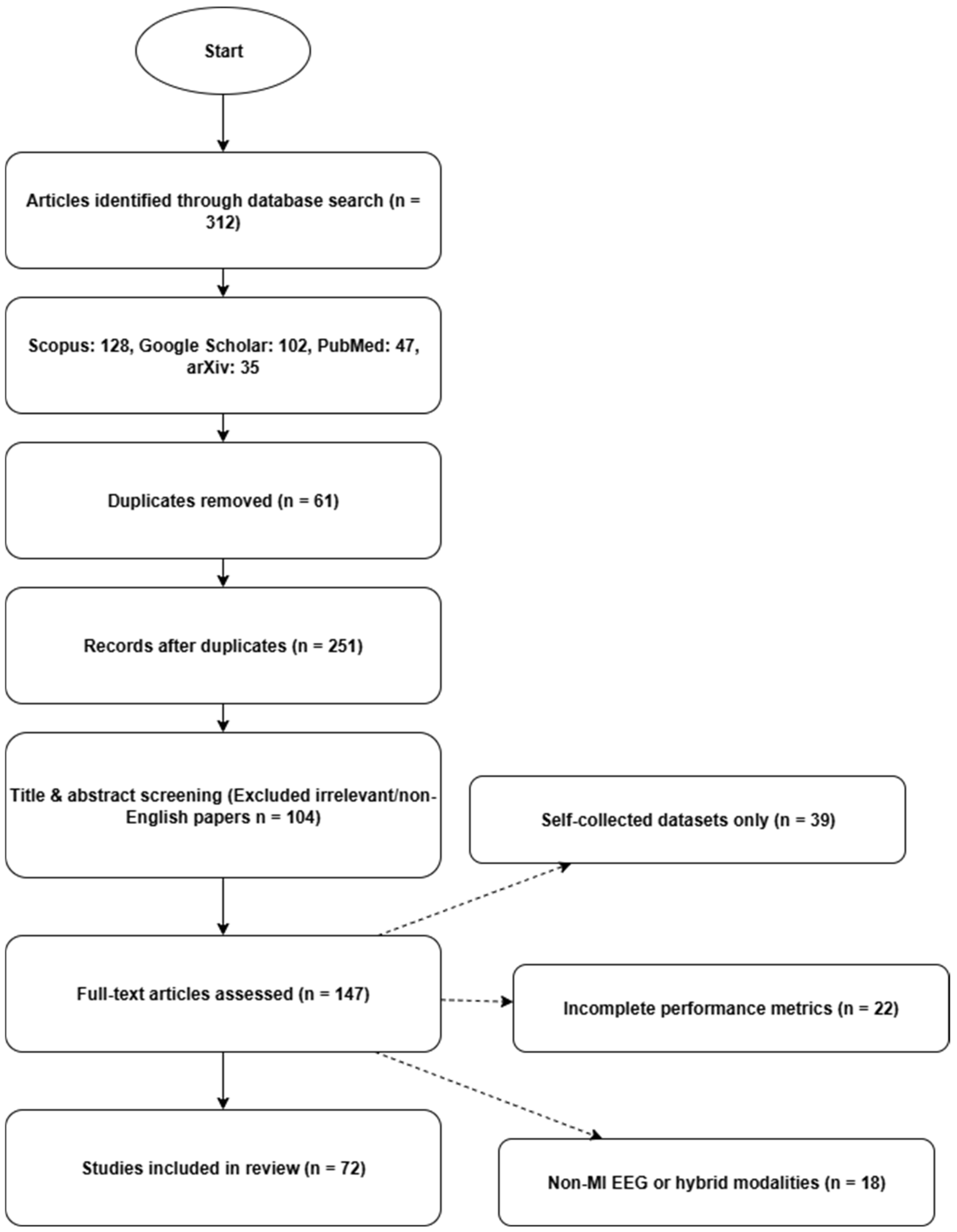
Figure 1. Protocol for the retrieval of papers.
Applsci 15 12075 g001
Figure 2. Electrode placement for recording EEG signals [35]. This figure shows (a) a 10–10 electrode placement system (Bold: 10–20 system), (b) The Cerebral lobes and central area, and (c) the placement configuration of the 16 electrodes.
Applsci 15 12075 g002
Figure 3. Classical, current, and modern BCI eras.
Applsci 15 12075 g003
Figure 4. BCI architecture [39].
Applsci 15 12075 g004
Figure 5. SVM optimal hyperplane with two classes [64].
Applsci 15 12075 g005
Figure 7. Convolutional neural network architecture [70].
Applsci 15 12075 g007
Figure 8. Layer-wise convolutional neural network architecture [72].
Applsci 15 12075 g008
Figure 9. PCNN block diagram [27].
Applsci 15 12075 g009
Figure 10. A hybrid CNN model for classification of motor tasks obtained from a hybrid BCI system [75].
Applsci 15 12075 g010
Figure 11. Performance evaluation based on the dataset. This figure illustrates the performance of the datasets based on different classifiers used.
Applsci 15 12075 g011
Figure 12. Performance evaluation based on classes. The figure illustrates the performance of the system based on class size when complexity is increased.
Applsci 15 12075 g012
Figure 13. Performance evaluation based on the decomposition methods used.
Applsci 15 12075 g013
Figure 14. Performance evaluation based on the feature extraction methods used.
Applsci 15 12075 g014
Figure 15. Performance evaluation based on the combined methods used.
Applsci 15 12075 g015
Figure 16. Evaluation metrics based on precision, recall, and F1 score.
Applsci 15 12075 g016
Table 1. This table shows a summary of the literature review.
YearAuthorsDatasetsMethodsPerformanceStudy LimitationFindings
2023W. Huang et al. [16]Physio Net
and GigaDB
RP-BCNNs91%Possibility of spatial information loss.Suitable for learning nonlinear dynamic features
2024R. Agrawal et al. [18]Self-generatedCSP + EMD + DNN97%Computational complexity and noise susceptibilityLab and real-time deployment analysis
2024W. Hu et al. [19]BCI IV-1aPSD + CSP + SVM91.43%Cross-subject variability
Not fully explored
Improved binary MI accuracy
2022M.J. Antony [20]BCI IV-2aAdaptive SVM
Adaptive LDA
91%
86%
Limited to online analysis, no real-world validationOptimized classification accuracy
2020V.K. Mehla et al. [21]-EMD + SVM95%Subject-to-subject variation Strong pattern recognition
2022Hai Hu et al. [22]BCI IV-1a and IIICiSSA + CSP96%High-dimensional feature
space, leads to overfitting
Highly effective feature extraction
2025M.S. Sagahab [23]Self-generatedHjorth parameters92.05%Small sample size,
generalization limited
Interpretable neural
features
2020Miao M et al. [24]BCI III-4,
private
CSP + CNN90%Limited subject dataAutomatic spatial frequency feature learning
2020Xu et al. [25]BCI IV-2aFBCSP + SVM78.50%Intra-subject variabilityHigh-accuracy multi-view fusion
Table 2. This table shows the dataset overview.
DatasetsSubjectChannelsAge and Sex (F or M)Sampling
Rate
ClassStudy Limitation
BCI Competition
IV 2a and 2b [27]
922-2502 ClassInter-subject variation, possibility of overfitting, and high computation
4 Class
BCI Competition
IV 2a and 2b [28]
922-2502 ClassLimited generalization beyond BCI datasets and subjects
BCI Competition
IV 2a and 2b [29]
922-2502 ClassHigh model complexity, generalization validated
4 Class
BCI Competition
IV 2a and 2b [30]
922-2502 ClassSensitive to low SNR and session-to-session variation, with limited real-world validation
4 Class
Physio Net [31]10964-1602 Class (E*)Low SNR and session variability may reduce generalization
4 Class (I*)
Physio Net [32]10 and 30--1602 ClassAccuracy drops in multi-class tasks, inter-session variability
4 Class
Physio Net [33]----2 ClassLimited to offline analysis
Physio Net [34]5722-2502 ClassModel performance may vary across different user groups; real-world applicability was not fully validated.
E*: Executed, I*: imagined.
Table 3. The summary of dataset characteristics based on BCI competition IV 2a and 2b and PhysioNet.
DatasetsSubjectsClasses *Recording DurationTrails per Class
BCI Competition IV 2a94 (LH, RH, F, T)~288 trials per subject72/class
BCI Competition IV 2b92 (LH, RH)~160 trials per subject80/class
PhysioNet EEG Motor Movement/Imagery 1092 (LH, RH) + variants~150 trials per subject75/class
Or 4 (LH, RH, F, T)
* LH: left hand; RH: right hand; F: foot; T: tongue.
Table 4. Summary of system performance based on different methods.
DatasetPreprocessingFeature ExtractionClassifierAccuracy (%)Notes
BCI Competition
IV 2a [27]
Bandpass + Notch filterEMDPCNN99.1%
(2-class)
Strong robustness via IMF decomposition
BCI Competition
IV 2b [27]
Bandpass + Notch filter EMDPCNN99.39%
(4-class)
Effective multiclass separation
BCI Competition
IV 2a [28]
Bandpass + Notch filterBand-power + HjorthLDA93.6%
(2-class)
Good spectral + temporal fusion
BCI Competition
IV 2b [28]
Bandpass + Notch filterBand-power + HjorthLDA87.8%
(2-class)
Drop in generalization across sessions
BCI Competition
IV 2a [29]
-Raw EEG (Conv Input)CNN 88.4%
(2-class)
CNN learns hierarchical features
BCI Competition
IV 2b [29]
-Raw EEG (Conv Input)CNN88.6%
(4-class)
Small improvement despite higher class count
BCI Competition
IV 2a [30]
Bandpass + Notch filterCSPSVM73.2%
(2-class)
Margin-based separation but low robustness
BCI Competition
IV 2b [30]
Bandpass + Notch filterCSPSVM70.1%
(4-class)
Multi-class setting stresses CSP
Physio Net [31]-CNN (Executed MI)CNN89.6%
(2-class)
Executed tasks give stronger discriminative patterns
Physio Net [31]-CNN (imagined MI)CNN87.8%
(2-class)
Imagined tasks are harder to classify
Physio Net [32]Butterworth + sliding window-PCNN99.73%
(2-class)
Very high binary accuracy
Physio Net [32]Butterworth + sliding window-PCNN83.37%
(4-class)
Accuracy drops with increased complexity
Physio Net [33]-CSPSVM97.1%
(2-class)
Strong linear separation under controlled setup
Physio Net [34]-CSPLDA64.45%
(2-class)
Performance is limited by electrode coverage
Table 5. Advantages and limitations of BCI methods.
MethodAdvantagesLimitations
FIR/IIR FiltersSimple, fast, and effective for removing line noise and band-limiting EEGLimited to fixed frequency bands, cannot adapt to nonstationary signals
ICASeparate sources and remove eye blinks/muscle artifacts effectivelyPerformance depends on channel count and noise, and is unstable across subjects.
CNN/Parallel CNNLearns spatial–temporal patterns directly, achieves high accuracies (95–99%)Requires large datasets, may overfit if the data are limited.
AutoencodersUnsupervised denoising compresses features efficientlyReconstruction may lose subtle EEG features and requires fine-tuning.
GANsCan generate a realistic synthetic EEG to balance training sets.Prone to instability in training, risk of mode collapse.
RNN/LSTM/GRUCaptures temporal dependencies across long EEG sequencesTraining is slow, high computational demand, sensitive to vanishing gradients.
Transformers Excellent for capturing global dependencies, promising in EEG-BCI.Requires massive datasets, still relatively unexplored for BCI
Hybrid (EMD + CNN, CSP + LSTM)Combines feature decomposition with deep learning, achieving state-of-the-art accuracies (>99%)Increased computational cost, risk of overfitting on small datasets.
Disclaimer/Publisher’s Note: The statements, opinions and data contained in all publications are solely those of the individual author(s) and contributor(s) and not of MDPI and/or the editor(s). MDPI and/or the editor(s) disclaim responsibility for any injury to people or property resulting from any ideas, methods, instructions or products referred to in the content.