Article

Predicting the Strength of Fly Ash–Slag–Gypsum-Based Backfill Materials Using Interpretable Machine Learning Modeling

1
School of Resource and Safety Engineering, University of Science and Technology Beijing, Beijing 100083, China
2
Institute of Mineral Resources, University of Science and Technology Beijing, Beijing 100083, China
*
Author to whom correspondence should be addressed.
Appl. Sci. 2025, 15(22), 12035; https://doi.org/10.3390/app152212035
Submission received: 2 October 2025 / Revised: 1 November 2025 / Accepted: 10 November 2025 / Published: 12 November 2025

Featured Application

Application of interpretable machine learning models for the strength prediction of filling materials.

Abstract

Predicting unconfined compressive strength (UCS) is essential for the safety and stability of solid waste-based backfill materials, particularly due to the correlation between strength development and hazardous substance immobilization. This study developed a machine learning model to predict UCS and optimize mixtures using fly ash, slag, and desulfurized gypsum. A dataset with 14 input features—including composition, water content, and curing time—was analyzed using Recursive Feature Elimination (RFE) for feature selection. Random Forest, Bayesian, and Gray Wolf Optimizer (GWO)-enhanced models were compared. The GWO-GB model achieved superior accuracy (R2 = 0.9335), with curing time (27.99%), water content (22.16%), and sulfur trioxide (18.98%) identified as the most significant features. The model enables rapid, high-precision UCS prediction, reduces experimental workload, and offers insights for mix design optimization and feature interaction analysis.

1. Introduction

With the growth of the population and the improvement of living standards, the production of municipal solid waste (MSW) continues to rise [1,2]. Addressing the increasingly severe urban environmental issues requires integrating sustainable infrastructure into urban development plans, which is crucial for achieving a sustainable urban transformation [3]. The conflict between green materials and ecology can be effectively mitigated through cost-effective and environmentally friendly technologies, such as the utilization of materials and waste recycling, thereby promoting the development of more sustainable cities [4,5]. Incineration has become the mainstream method for treating MSW, which not only reduces waste volume and recovers energy but also inevitably produces substantial amounts of incineration residues, primarily bottom ash (MSWIBA) and fly ash (MSWIFA) [6,7,8]. As a secondary waste, the disposal and utilization of MSWIFA remain significant challenges in urban management and sustainable development.
With advancements in cementitious materials science, alternative approaches have emerged that replace traditional binders like cement with solid waste materials possessing latent cementitious properties, such as fly ash, steel slag, and blast furnace slag [9,10,11]. The primary components of MSWIFA are similar to those of pulverized coal fly ash and slag [12,13], mainly consisting of SiO2, CaCO3, Al2O3, and Fe2O3. Additionally, due to high-temperature calcination and cooling, MSWIFA contains glassy phases that exhibit some degree of pozzolanic reactivity [14], making it suitable as a supplementary raw material in cementitious systems. As a result, the application of MSWIFA in mine backfill has become a hotspot for efficient waste utilization and the development of solid waste-based backfill materials. In backfill systems containing slag, MSWIFA has been shown to activate slag hydration, promoting the formation of C–S–H gels and hydrated calcium chloroaluminate [15,16]. The formation of C–S–H gels is closely related to compressive strength and plays a crucial role in the adsorption and immobilization of hazardous substances [17]. Li et al. [18] found that when the MSWIFA content reached 70%, the optimized formulation achieved a compressive strength of 11.97 MPa, with heavy metal immobilization rates above 92%, and the cured products exhibited favorable durability. These findings highlight the positive role of MSWIFA in enhancing the strength and environmental performance of slag-desulfurized gypsum-based low-carbon cementitious mine backfill materials.
The compressive strength of backfill materials is a key factor influencing the safety and stability of backfill operations [19]. In underground mining environments, different stope locations require varying strength specifications for backfill materials, and the strength of the material is positively correlated with its capacity to immobilize hazardous substances [20,21]. Therefore, accurately predicting uniaxial compressive strength (UCS) is critical to ensuring the safety of mining operations. Due to the dynamic variations in composition, dosage, and processing parameters of various solid waste materials [22,23,24], the ability to promptly and accurately predict the strength of backfill materials made from these raw components is crucial for maintaining both operational stability and the safety of backfill operations.
In recent years, machine learning (ML) has emerged as a powerful tool for material performance prediction, owing to its ability to accurately model complex, nonlinear relationships between input parameters and output properties [25,26]. Researchers have developed single models (e.g., artificial neural networks, ANNs) and ensemble models (e.g., gradient boosting, random forests) to predict the mechanical behavior of cementitious materials across diverse systems [27,28]. For instance, Chathuranga et al. [29] compared the predictive performance of support vector regression (SVR), artificial neural networks (ANNs), and an ensemble gradient boosting regression model for the unconfined compressive strength (UCS) of alkali-activated slag-based cemented paste backfill (AAS-based CPB). Their findings demonstrated that the ensemble model outperformed individual models in accuracy. Similarly, Cheng et al. [30] constructed a convolutional neural network (CNN) using coarse aggregate, fine aggregate, and binder composition as input features to rapidly predict the strength of paste backfill materials with varying mix proportions. Further advancing predictive capabilities, Qi et al. [31] established a global UCS dataset comprising 986 experimental samples derived from the literature and laboratory studies. Through hyperparameter optimization, their deep neural network (DNN) model (with 4 hidden layers, a learning rate of 0.001, and a dropout rate of 0.25) achieved an R2 of 0.967 on the test set, confirming its high predictive reliability for CPB UCS. To further enhance model accuracy, intelligent hyperparameter tuning and feature selection strategies have been integrated. Zhang et al. [32] developed a hybrid DNN–genetic algorithm (GA) framework for strength prediction and mix design optimization of ultra-fine tailings-based backfill, significantly improving model adaptability. Hu et al. [33] employed an extreme learning machine (ELM) optimized by a sparrow search algorithm (SSA), achieving a 5.4% increase in R2, a 46.3% reduction in RMSE, and a 12.8% improvement in VAF (variance accounted for), demonstrating superior predictive precision for backfill UCS. Additionally, Qiu et al. [34] systematically investigated the influence of concentration, ash–sand ratio, waste rock ratio, curing time, and temperature on backfill UCS using 174 experimental datasets. Their AEO-CatBoost model (optimized with a population size of 60) yielded optimal performance (R2 = 0.947, RMSE = 0.606, MAE = 0.465, VAF = 93.614), and SHAP (SHapley Additive exPlanations) analysis was applied to elucidate the microstructural–macroscopic mechanical property relationships. Given the complexity of solid waste-based backfill materials, where raw material compositions and interactions are far more intricate than in traditional cement systems, tailored predictive models and mechanistic interpretations are essential. In particular, the variability among different filling materials and datasets calls for comprehensive studies that include feature selection, performance prediction, and model interpretability to unravel the fundamental factors influencing material behavior. This study focuses on strength prediction and model interpretability for fly ash–slag–desulfurization gypsum (FSDG)-based backfill materials, aiming to uncover the key governing factors affecting their performance.
Accordingly, this study focuses on compressive strength prediction for fly ash-slag-desulfurized gypsum (FSDG)-based backfill materials. We propose an interpretable machine learning framework, RFE-GWO-GBDT, to enhance prediction accuracy and model interpretability. First, a comprehensive database was established by collecting 153 experimental datasets from the literature, including raw material compositions (fly ash, slag, desulfurized gypsum, tailings), mix proportions, curing time, and compressive strength. Based on this dataset, four baseline models (including Random Forest, RF) were constructed. To optimize feature selection, Recursive Feature Elimination (RFE) was employed to identify the most influential predictors. Subsequently, four optimization algorithms (including Bayesian Optimization, BO, and Whale Optimization Algorithm, WOA) were applied to tune hyperparameters for improved model performance. The predictive performance of the models was rigorously evaluated using four metrics: R2 (coefficient of determination), MAE (mean absolute error), MSE (mean squared error), and RAE (relative absolute error). The optimal model was selected based on these metrics. Furthermore, SHAP (SHapley Additive exPlanations) analysis and partial dependence plots (PDPs) were utilized to interpret feature contributions, revealing the interaction mechanisms between input features and compressive strength, and the threshold values at which each feature positively influences the UCS (unconfined compressive strength). By utilizing the RFE-GWO-GB model, high-precision predictions were achieved within a short period, significantly reducing the experimental cycle and research effort. The model interpretation provides guidance for mix design experiments of cementitious materials prepared from various solid wastes, identifies the threshold values at which features positively contribute to strength, and reveals the dynamic interaction patterns among the input features. Finally, Figure 1 provides a systematic visualization of the end-to-end machine learning framework for strength prediction, integrating sequential stages of data collection, feature selection, model optimization, performance assessment, and mechanistic interpretability analysis.

2. Materials and Methods

The fly ash used in this study was sourced from a municipal solid waste incineration plant in Beijing, where it was processed using a mechanical grate incineration technology. Its physical properties were measured, revealing a specific surface area of 374 m2/kg. The cementitious material, slag, was obtained from a company in Hebei Province, with a specific surface area of 500 m2/kg. The iron tailings used in the tests were also collected from a company in Hebei Province. Their particle size distribution was analyzed using a laser particle size analyzer, and the cumulative distribution percentiles were found to be D10 = 3.29 μm, D50 = 21.7 μm, and D90 = 69.3 μm. The chemical compositions of all raw materials were determined using X-ray fluorescence (XRF) spectroscopy, as shown in Table 1.

2.1. Data Collection

A database comprising 163 datasets was established by integrating experimental data on backfill material preparation accumulated by the research team and data retrieved from the team’s previously published studies [15,21,35,36]. This database encompasses key features including the chemical composition of raw materials (determined via X-ray fluorescence, XRF), raw material dosages (in grams), slurry concentrations (expressed as mass percentages), and compressive strength metrics. Both the referenced literature data and experimental datasets were obtained under standardized curing conditions (22 °C in a standard curing chamber with 95% humidity) using identical testing facilities (BC-100D stress testing machine). Prior to analysis, the dataset underwent rigorous preprocessing: rows containing missing values were removed to ensure data integrity, infinite values were converted to NaN (Not a Number) followed by deletion of corresponding rows to mitigate outlier interference. The final 153 preprocessed datasets were standardized to enhance model convergence efficiency and predictive performance, thereby indirectly reinforcing model stability. The dataset was then randomly partitioned into training (70%) and testing (30%) subsets at a 7:3 ratio.
Comprehensive statistical analysis was conducted on the curated dataset to characterize data distribution, calculating key descriptors including mean, minimum, maximum, median, standard deviation, 25th percentile (Q25%), and 75th percentile (Q75%)—results are summarized in Table 2.
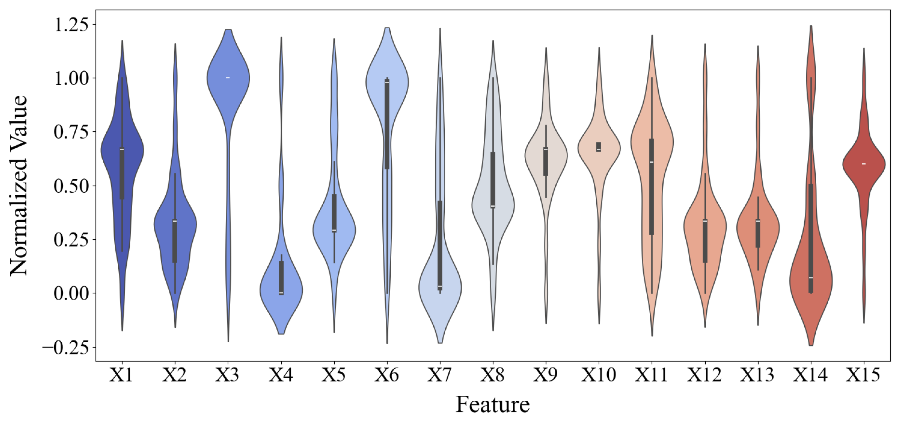
To eliminate the dimensional differences between data features and standardize the data scale to ensure model performance, this study used the “StandardScaler” module from scikit-learn to perform standardization on both the training and testing sets. The standardization process scaled the feature values to a standard normal distribution with a mean of 0 and a standard deviation of 1. The distribution of the standardized data is shown in Figure 2. As can be seen, the data distribution closely resembles a normal distribution, with the data being relatively concentrated, thus meeting the standard for the database.
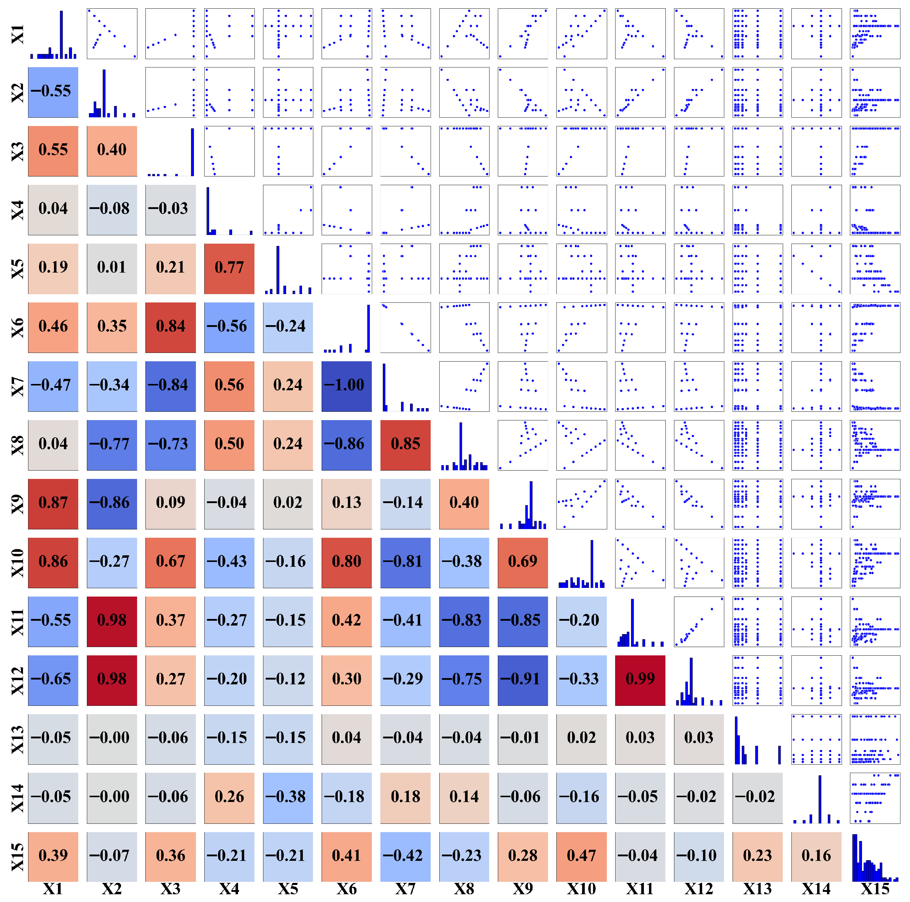
A total of 15 features were collected in this study, comprising 14 input features and 1 output feature (compressive strength). To evaluate the interrelationships among input features and their correlations with compressive strength, the Pearson correlation coefficient matrix was computed using the X.corr() function from the pandas library in Python. The Pearson correlation coefficient quantifies the linear relationship between two features, with values ranging from −1 to 1 [37]. As illustrated in Figure 3, the lower triangular portion of the matrix reveals a perfect negative correlation between feature X6 (calcium oxide) and X7 (iron oxide), indicating a strict inverse linear relationship. Furthermore, X12 (potassium sodium oxide) and X13 (curing time), X10 (sulfur trioxide) and X11 (chlorine), along with X8 (silicon dioxide) and X9 (aluminum oxide) exhibit strong positive correlations, suggesting significant linear dependencies among these features. These pronounced correlations stem from the specific proportions of solid waste materials used. Regarding material composition, moderate correlations were observed between X1 (slag) and X2 (fly ash), and between X3 (desulfurization gypsum) and X4 (tailings), whereas negligible correlations were found between X1 (slag) and X4 (tailings), and between X2 (fly ash) and X4 (tailings), reflecting the intricate network of relationships among features in the dataset.

2.2. Model Introduction

To select the best predictive model, this study compared different paradigms of ensemble learning models with neural network models. This included the Random Forest (RF) from the Bagging model, the classic Gradient Boosting (GB) and LightGBM (LGBM) from the Boosting model, and the Convolutional Neural Network (CNN) from the neural network models, which demonstrated excellent performance. All models and algorithms were implemented based on Python 3.12.1. To ensure uniformity in the randomness during the experiment and the reproducibility of the results, the ‘random_state’ parameter for all relevant models was fixed at 0.

2.2.1. Random Forest

Random Forest is an ensemble learning method that enhances prediction accuracy and controls overfitting by constructing multiple decision trees and combining their predicted results [38]. Each decision tree is trained on a different training sample set generated by bootstrapping from the original dataset, which increases the model’s diversity and helps reduce variance [29]. During the construction of each tree, not all features are considered for the optimal split; instead, a random subset of features is selected for splitting, further enhancing the diversity between trees and improving the overall stability and accuracy of the model.

2.2.2. Gradient Boosting

GBDT, or Gradient Boosting Decision Tree, is an ensemble learning method primarily used for regression and classification tasks. It builds a strong learner by combining multiple weak learners, typically simple decision trees. The core idea of GBDT is to iteratively train a series of decision trees, where each tree attempts to correct the prediction errors made by the previous tree [39].

2.2.3. LightGBM

LGBM, or LightGBM (Light Gradient Boosting Machine), is a gradient boosting framework based on decision tree algorithms, developed by Microsoft. It is specifically designed to improve the speed and efficiency of traditional gradient boosting methods while maintaining high accuracy. LightGBM performs exceptionally well when handling large-scale datasets and is capable of managing memory usage effectively [40].

2.2.4. CNN

The core idea of CNN (Convolutional Neural Network) is to automatically extract low-level features with strong local correlations from the input data through convolution operations. By stacking and combining multiple layers of convolutional structures, CNN gradually abstracts more representative and semantically meaningful high-level features [41]. The convolutional layers close to the input typically capture basic local patterns, while intermediate layers further integrate these local features to form more complex texture combinations, simple shapes, or local structures. The higher convolutional layers capture more global, abstract semantic information and overall structures from the data, which are often more directly related to the final prediction target. During the prediction phase, the trained CNN model has learned a stable mapping relationship between the input data and the target output. The core objective is to perform forward propagation of new input samples through the pre-trained network structure to output the corresponding prediction results [42]. Unlike the training phase, the prediction process does not require gradient calculations or model parameter updates. Instead, it only requires the use of fixed network weights to complete feature extraction and mapping, enabling efficient and stable inference and decision-making.

2.3. Algorithm Introduction

Using algorithms to optimize model parameters and reduce local optima is a critical step. The essence of machine learning and deep learning model prediction performance is an optimization problem, which involves minimizing the error between predicted and actual test values [43]. Swarm intelligence algorithms simulate the search behaviors of biological organisms, leveraging the learning experiences of individuals and the group to find the optimal prediction values. Through parallel searches conducted by multiple individuals within the group, these algorithms can cover a broader region of the solution space, effectively avoiding premature convergence to local optima during the optimization process.

2.3.1. Bayesian Optimization

Bayesian Optimization (BO) algorithm selects the optimal hyperparameters by constructing a surrogate function and modeling the conditional probability of the performance on the validation set. BO tracks all historical evaluation data and uses an acquisition function to identify the hyperparameter combinations that are most likely to improve model performance in the next iteration, thereby enabling efficient exploration [44]. When applying the BO algorithm strategy in a dynamic ensemble module to search for optimal hyperparameters, this method achieves higher tuning accuracy and efficiency in a shorter evaluation time. Compared to traditional grid search or random search methods, BO not only significantly enhances tuning efficiency but also avoids the waste of computational resources caused by poorly evaluated hyperparameters.

2.3.2. Gray Wolf Algorithm

The Gray Wolf Optimizer (GWO) is a metaheuristic optimization method that simulates the social hierarchy and cooperative mechanisms within a gray wolf pack to achieve global optimization. In the GWO algorithm, individuals in the population are divided into four main social levels: alpha (α), beta (β), delta (δ), and omega (ω), each of which plays a distinct role in the optimization process. These wolves at different levels collaborate and compete by mimicking natural hunting behaviors, gradually converging towards the global optimum. Each wolf adjusts its search strategy based on its relative position to the Alpha, Beta, and Delta wolves, thus achieving an effective balance between exploration and exploitation across the solution space [45]. Additionally, the GWO algorithm dynamically adjusts the search step size and direction, further enhancing its adaptability and flexibility, which enables it to perform exceptionally well in handling complex, multimodal optimization problems. In this study, the GWO algorithm parameters were configured with a population size (n_wolves) of 10, representing 10 “gray wolves” participating in the search for optimal solutions per generation, where each individual represents a unique combination of hyperparameters to be optimized. The maximum number of iterations (n_iter) was set to 10, meaning the optimization process comprised 10 iterative rounds, with the positions of all wolves (candidate solutions) updated in each round.

2.3.3. Whale Optimization Algorithm

The Whale Optimization Algorithm (WOA) is an innovative metaheuristic optimization algorithm that achieves global optimization by simulating three continuous steps: encircling prey, creating a spiral bubble net to capture prey, and locating the next target. First, WOA mimics the behavior of humpback whales encircling their prey by adjusting the positions of candidate solutions to move closer to the current optimal solution, gradually narrowing the search space. Next, WOA generates a spiral movement around the current optimal solution using a mathematical model, replicating the process of humpback whales creating bubble nets. This unique search path increases the probability of finding better solutions. Finally, by dynamically adjusting the search direction and step size, WOA locates new potential optimal solutions. This process combines randomness and adaptive strategies to ensure continuous, efficient searching in complex and dynamic solution spaces [46]. WOA has demonstrated exceptional performance, particularly in handling high-dimensional complex optimization problems. Its enhanced exploration capability and ability to exploit local optima enable it to avoid getting trapped in local minima and rapidly converge to the global optimum. In this study, the core parameters of the Whale Optimization Algorithm (WOA) were configured as follows: population size (n_whales) was set to 10, representing 10 candidate solutions (whale individuals) searched simultaneously per generation, which influences global search capability and computational overhead; maximum iteration count (n_iter) was set to 10, defining 10 iterative rounds where candidate solution positions are updated each round to approach the optimal solution, determining optimization depth and computational time; optimization parameter dimension (dim) was set to 8, corresponding to 8 hyperparameters to be optimized, equivalent to the feature vector length of each candidate solution (whale); dynamic control parameter (a) was linearly decreased from 2.0 to 0.0 through the formula a = 2 − iter × (2/niter), regulating coefficients A and C to balance global exploration and local exploitation, with values dynamically generated during the iterative process.

2.3.4. Particle Swarm Algorithm

Particle Swarm Optimization (PSO) is a metaheuristic optimization algorithm based on swarm intelligence, inspired by the social dynamics of biological groups in nature, such as schools of fish and flocks of birds. It was proposed by Kennedy and Eberhart in the mid-1990s, aiming to solve complex optimization problems by simulating the collaboration and information-sharing mechanisms between individual particles in a group. In PSO, a set of possible solutions is abstracted as “particles”, which dynamically search the multi-dimensional solution space to find the global optimum [47]. Each particle adjusts its trajectory based on its own experience (i.e., personal best position, pbest) and the collective experience of the swarm (i.e., global best position, gbest). The velocity and position of the particles are continuously updated using mathematical models, achieving an efficient balance between exploration and exploitation in the solution space [48]. This mechanism allows PSO to handle highly nonlinear, non-convex, or black-box optimization problems without requiring gradient information, demonstrating great flexibility and adaptability.

2.3.5. Recursive Feature Elimination

In the process of feature selection in machine learning, Recursive Feature Elimination (RFE) is a model-based feature selection algorithm that iteratively trains a model and removes the least important features to select the optimal subset of features. The core mechanism of the RFE algorithm is as follows: first, the selected base model is trained on the current set of features; then, based on the feature importance or coefficients provided by the model, the contribution of each feature to the model’s prediction ability is assessed. Next, the least important feature is eliminated, and the feature set is updated. This process is repeated until the desired number of features is reached or other stopping criteria are met [49]. This method effectively reduces the number of features step by step and ranks them based on their importance to the model, ultimately producing an optimized feature set. This process not only helps reduce the dimensionality of the feature space and mitigates the risk of overfitting, but also enhances the interpretability of the model, allowing researchers to better understand which features have a critical impact on the prediction results.

3. Results and Discussion

3.1. Results of Feature Parameter Selection

The results of feature selection through Recursive Feature Elimination (RFE) combined with each model, along with the model parameters, are shown in Table 3. Among the four models, curing time, slag, aluminum oxide, and sulfur trioxide are consistently included as core features, highlighting their pivotal role in prediction. Additionally, water, calcium oxide, iron(III) oxide, chlorine, and concentration emerge as high-frequency features that significantly influence prediction outcomes. In contrast, less influential features such as fly ash and tailings were selectively incorporated only by the LGBM and CNN models. Overall, the selected features across models demonstrate considerable similarity and concentration, with comparable rankings in feature importance. All models adopt early stopping as the training termination criterion: training halts when validation set performance (e.g., MSE) fails to improve for a predefined number of consecutive epochs (patience), effectively preventing overfitting while balancing model convergence with computational efficiency.

3.2. Model Evaluation Results

The model performance was evaluated using multiple metrics to ensure stable assessment. To ensure consistent evaluation, a 5-fold cross-validation method was employed in the study. The metrics include the coefficient of determination (R2) as shown in Equation (1), Root Mean Squared Error (RMSE) as shown in Equation (2), Mean Absolute Error (MAE) as shown in Equation (3), and Relative Absolute Error (RAE) as shown in Equation (4). In the evaluation of machine learning models, the coefficient of determination (R2) measures the model’s ability to explain the variance in the data. Its value ranges from 0 to 1, with values closer to 1 indicating better fit and higher explanatory power [49]. The Mean Absolute Error (MAE) quantifies the average absolute deviation between predicted and actual values, with smaller values indicating higher predictive accuracy [50]. Mean Squared Error (MSE) calculates the average squared error between predicted and actual values, being more sensitive to larger errors, and smaller values reflect better predictive performance [51]. RAE compares the sum of absolute errors between predicted and actual values with the sum of absolute errors between actual values and their mean, providing a relative measure of the model’s prediction capability [52]. These evaluation metrics reflect different aspects of the model’s performance. By using them collectively, a comprehensive and objective assessment of the model’s predictive ability and generalization performance can be achieved, providing a scientific basis for model selection and optimization.
R 2 = 1 i = 1 n y i y ^ i 2 | i = 1 n y i y 2
y i is the actual value, y ^ i is the predicted value, y is the average of the actual values, n is the sample size.
MSE = 1 n i = 1 n y i y ^ i 2
y i is the actual value, y ^ i is the predicted value, n is the sample size.
MAE = 1 n i = 1 n y i y ^ i
y i is the actual value, y ^ i is the predicted value, n is the sample size.
RAE = Σ y i ŷ i / Σ y i ȳ
y i is the actual value, ŷi is the predicted value of the ith observation, ȳ is the average of the actual values of all observations.
As shown in Table 4, integrating Grid Search (GS) with other models yields only marginal performance improvements. Specifically, when comparing GS-RF, GS-GB, and GS-LGBM with their corresponding baseline models (RF, GB, and LGBM), the test-set metrics—including R2, MAE, and MSE—demonstrate only slight enhancements, indicating limited overall improvement. In scenarios characterized by limited training data, high-dimensional feature spaces, and complex model parameter spaces, combining GS with these models may require more refined and targeted hyperparameter tuning to achieve optimal predictive performance. Furthermore, the limited performance gains observed when integrating GS with various models can be attributed to multiple factors, including the inherent complexity of the base models, the risk of overfitting, dataset-specific characteristics, and insufficient or suboptimal parameter optimization strategies. These elements collectively contribute to the observed modest improvements in model performance.
The performance of models using all 14 features combined with grid search for hyperparameter optimization is significantly inferior to that of models employing Recursive Feature Elimination (RFE) and intelligent optimization algorithms. Specifically, the four models exhibit lower R2 values on the training set compared to their counterparts, with the most notable difference observed between GS-GB (Grid Search applied to Gradient Boosting) and RFE-GWO-GBR (Recursive Feature Elimination combined with Gray Wolf Optimization applied to Gradient Boosting Regressor). In this comparison, the training set R2 of GS-GB is 0.13 lower than that of RFE-GWO-GBR, and its testing set R2 is 0.07 lower. Similar trends are evident across other models, indicating that incorporating feature selection (e.g., RFE) and advanced optimization strategies (e.g., GWO) enhances model generalization and predictive performance.
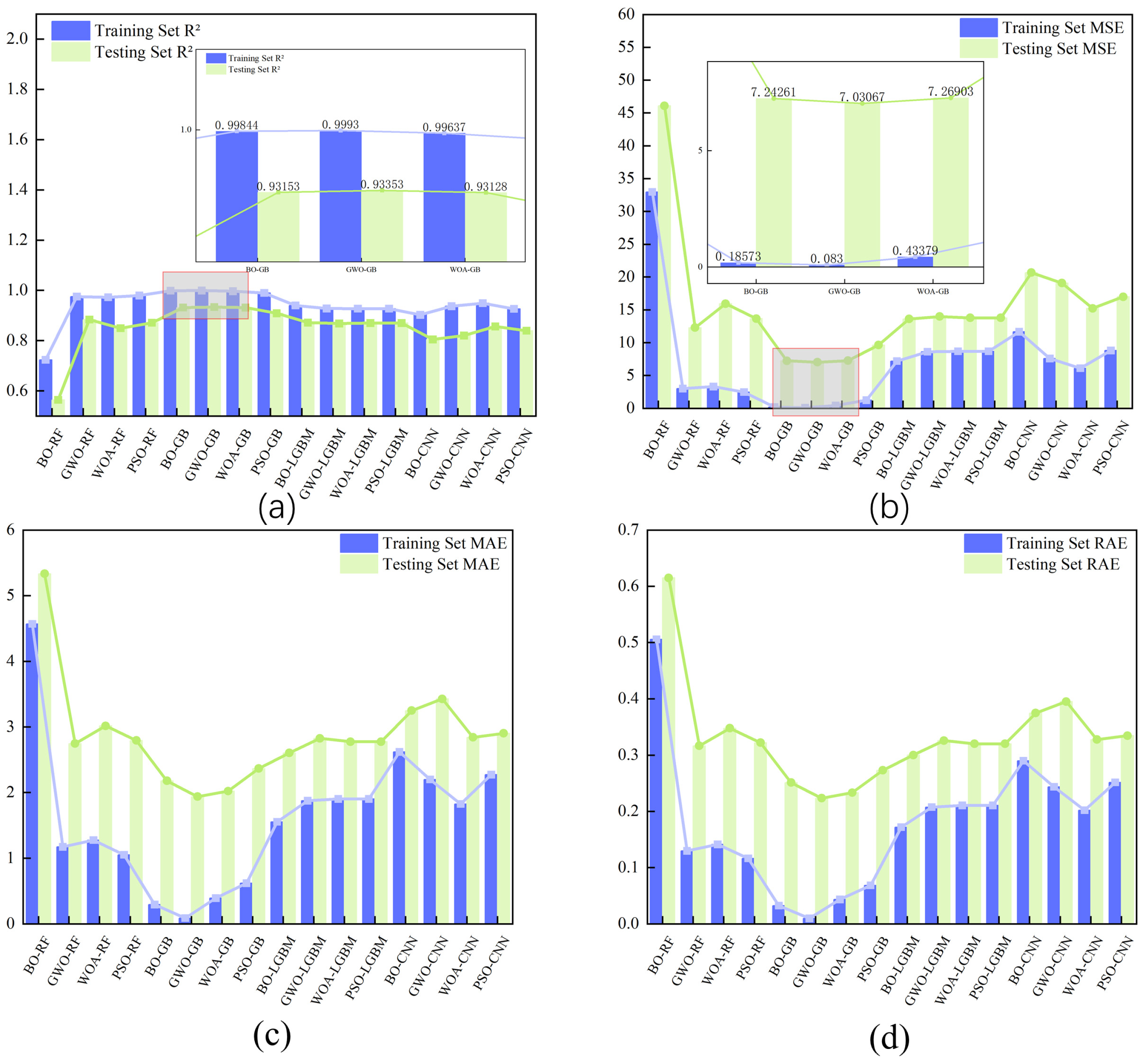
As shown in Figure 4, among the 16 combinations of optimization algorithms and machine learning models, the Gradient Boosting (GB) model demonstrates the best performance, with the coefficient of determination (R2) exceeding 0.9 across all optimization algorithms. The optimal algorithm-model combination is RFE-GWO-GB (test set R2 = 0.9335, MAE = 1.937 MPa, MSE = 7.031 MPa2, RAE = 0.223). Closely following is RFE-WOA-GB (test set R2 = 0.9313, MAE = 2.023 MPa, MSE = 7.269 MPa2, RAE = 0.233), which not only achieves a high R2 but also maintains low MAE and MSE, indicating excellent prediction performance and generalization ability after optimization with these two algorithms. In contrast, models such as RF, LightGBM, and CNN exhibit relatively weaker overall performance, with their generalization capabilities on the test set significantly lower than those of the GB model.
Gradient Boosting (GB) exhibits exceptional capabilities in nonlinear modeling and demonstrates high robustness to noise and outliers [53]. The model performs effectively in handling the complex relationships among material proportions, substance contents, and compressive strength, as well as managing high-dimensional data. Additionally, GB shows advantages with continuous numerical datasets, efficiently capturing feature interactions and nonlinear relationships. Proper normalization and feature selection further enhance its performance. Consequently, the model achieves near-perfect fitting on the training set (training set R2 ≈ 1.00) and maintains outstanding generalization on the test set. Evaluation metrics for the GB model indicate smaller prediction errors and higher goodness of fit, accurately reflecting variations in the target variable, which underscores its superiority in this specific dataset and modeling scenario.
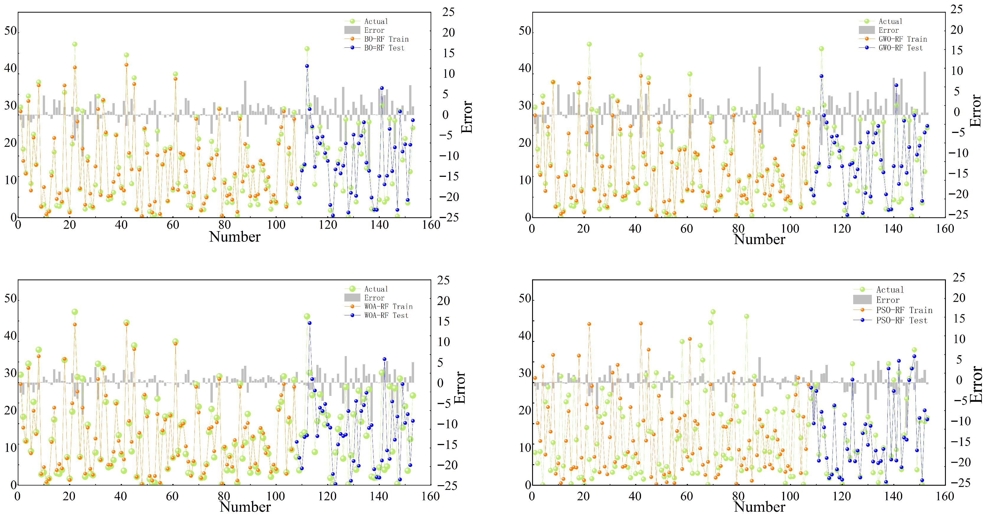
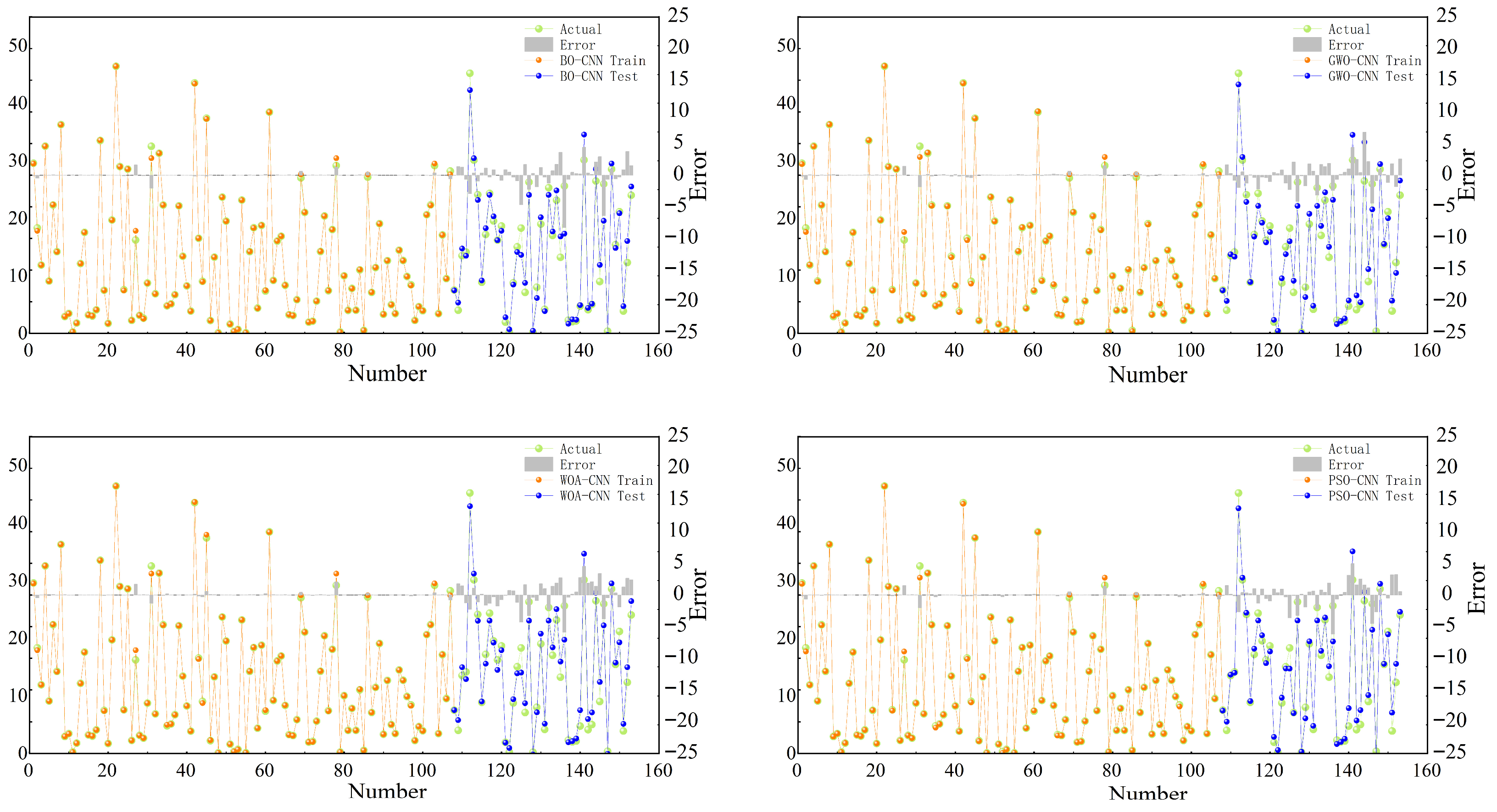
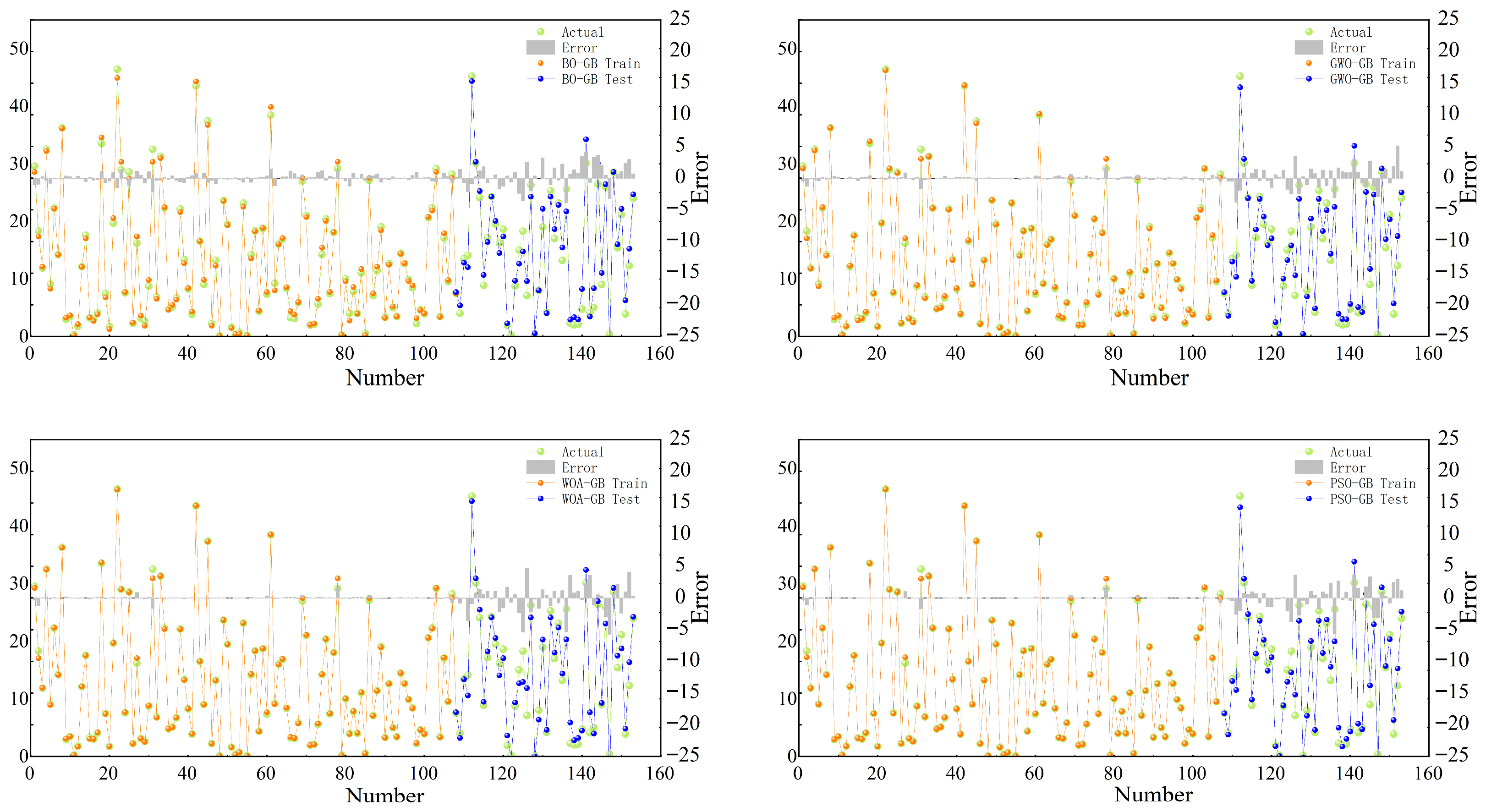
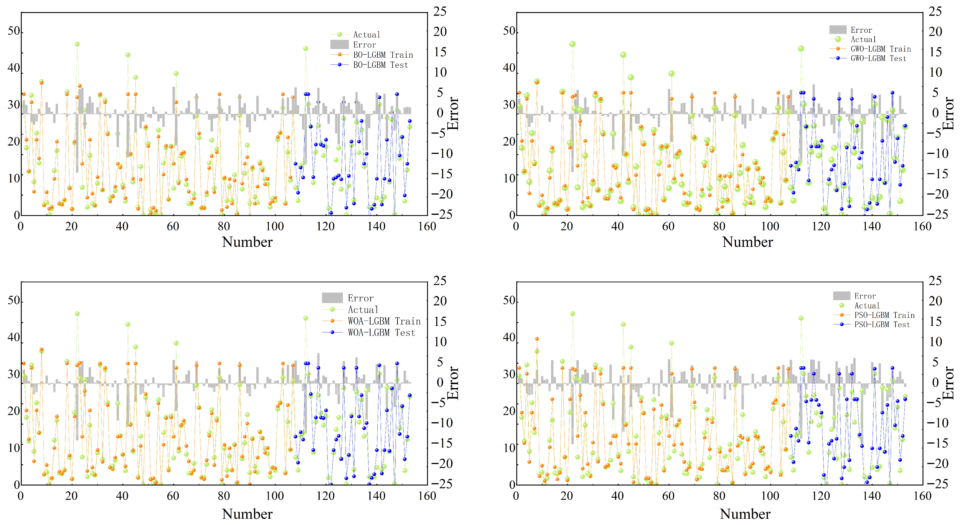
As shown in Figure 5, Figure 6, Figure 7 and Figure 8, the green dots represent the actual values, the gray bars represent the relative prediction errors, the orange dots indicate the predicted values on the training set, and the blue dots represent the predicted values on the test set. From Figure 5, it can be observed that the Particle Swarm Optimization (PSO) algorithm shows the worst optimization effect on the Random Forest (RF) model, followed by the Bayesian Optimization (BO) algorithm. This is evident from the low overlap between the training and testing set lines and the actual value lines. Additionally, from Table 4, it is clear that the average errors for the Particle Swarm and Bayesian algorithms on the training and testing sets are 1.05 MPa, 2.79 MPa, 4.57 MPa, and 5.33 MPa, respectively. After optimization with Gray Wolf Optimization (GWO) and Whale Optimization Algorithm (WOA), the RF model shows an improvement, with the average difference between the predicted and actual values in the test set being 2.75 MPa and 3.02 MPa, respectively, outperforming the previous two optimization algorithms.
In Figure 6, the performance of different optimization algorithms for the Convolutional Neural Network (CNN) model is shown. The results range from worst to best in the following order: Bayesian Optimization (BO), Particle Swarm Optimization (PSO), Gray Wolf Optimization (GWO), and Whale Optimization Algorithm (WOA). GWO and WOA achieve the lowest average errors on the test set, with values of 3.43 MPa and 2.84 MPa, respectively, demonstrating higher prediction accuracy and better fit.
Figure 7 illustrates the performance of different optimization algorithms on the Gradient Boosting (GB) model. It is evident that the optimization effect of Bayesian Optimization (BO) is the worst, while GWO and WOA provide the best results for optimizing the GB model. The average errors for the test set after optimization with GWO and WOA are 1.94 MPa and 2.02 MPa, respectively, indicating excellent performance. Moreover, Figure 8 shows that Whale Optimization Algorithm (WOA) performs exceptionally well and is well-suited for optimizing the LightGBM (LGBM) model, achieving a low average error of 2.84 MPa on the test set, with higher prediction accuracy and better fitting.
Among the compared optimization algorithms, GWO achieved the best performance in optimizing the four base models. The outstanding performance of the RFE-GWO-GB model can be attributed to the strong predictive capability of the base model, the efficiency of the optimization strategy, and its precise adaptation to the characteristics of the dataset. Given that the search space for optimal mix ratios—particularly the contents of raw materials such as slag, water, curing time, and alumina content—and their relationship with compressive strength is highly nonlinear, GWO effectively captured the nonlinear relationships between these key features and the strength response. As a result, the successful global-to-local search equilibrium achieved by GWO offers significant advantages over the iterative and locally focused strategy of Bayesian Optimization (BO), or the brute-force, swarm-like search mechanism of Particle Swarm Optimization (PSO). GWO mimics the social behavior of wolf packs by modeling the interactions among leaders (Alpha), followers (Beta), and boundary wolves (Delta) to guide the search process [54]. With minimal adjustable parameters, GWO is easy to implement and tune, and it can dynamically switch between global exploration and local exploitation. These properties make GWO a powerful global search algorithm that can effectively avoid local optima, exhibits strong adaptability, and is suitable for diverse data distributions and model architectures, thereby further enhancing the overall performance of the GB model.
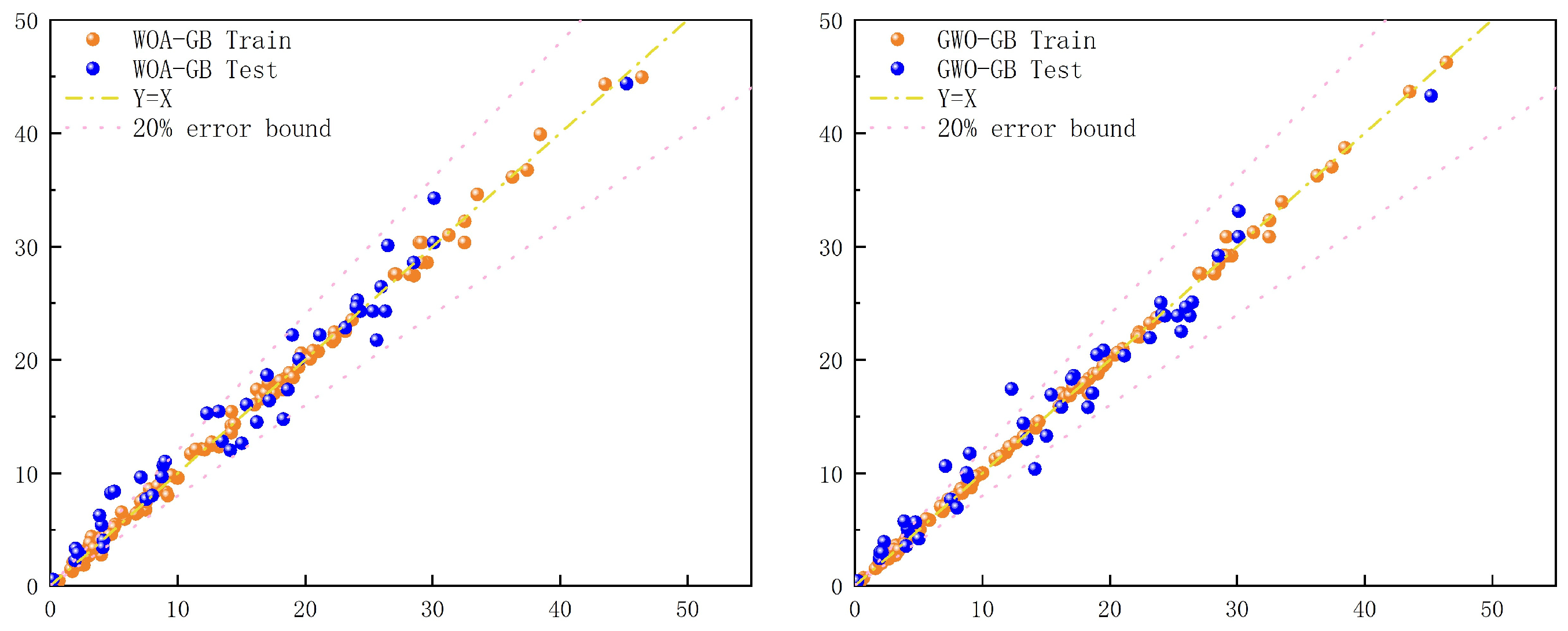
Figure 9 presents scatter comparison plots of model predicted values versus actual values, where the left panel corresponds to the (RFE-WOA-GB) model and the right panel to the (RFE-GWO-GB) model. In the figure, orange circles represent training set data, blue circles denote test set data, and green circles correspond to actual values; the dashed line Y = X indicates the ideal prediction state, while the dot-dashed line delineates the 20% error margin. The majority of data points are closely clustered around the Y = X line, with the vast majority falling within the 20% error margin, indicating a high degree of congruence between the predicted and actual values for both models. However, on the test set, the right panel demonstrates a closer alignment with the perfect prediction line. Combined with the data in Figure 3, it can be observed that under similar R2 values, the GWO-GB model exhibits lower MSE, MAE, and RAE, suggesting that the GWO-GB model may achieve higher prediction accuracy.

3.3. Validation

The raw materials (fly ash, slag, tailings, and water) are weighed according to the mix ratio, mixed into a uniform slurry, poured into 40 × 40 × 40 mm molds, compacted to remove air bubbles, and cured at 22 °C and 95% RH. The process is shown in Figure 10. To verify the prediction performance of the model, this study uses the most commonly used mix ratios from the experimental design. These include: slag 350 g, fly ash 100 g, desulfurized gypsum 50 g, water 600 g, and tailings 2000 g; slag 300 g, fly ash 150 g, desulfurized gypsum 50 g, water 600 g, and tailings 2000 g; slag 400 g, fly ash 50 g, desulfurized gypsum 50 g, water 600 g, and tailings 2000 g. After mixing, the slurry is poured into the mold and cured for 3, 7, and 28 days before performing compressive strength testing. At the same time, the corresponding mix ratios are input into the RFE-GWO-GB model for prediction. The experimental results show that the measured compressive strengths are 24.11 MPa, 18.32 MPa, 8.02 MPa, and 28.53 MPa, 26.31 MPa, 19.06 MPa, respectively, while the model predicted values are 24.03 MPa, 19.55 MPa, 9.23 MPa, and 29.18 MPa, 25.94 MPa, 18.67 MPa. The discrepancies between the actual samples and predicted values are small, indicating that the RFE-GWO-GB model has high accuracy in predicting the compressive strength of filling materials.

3.4. Optimal Model Interpretation

SHAP analysis facilitates the interpretation of machine learning model outputs by assigning each feature a value that quantifies its contribution to the prediction [40,55]. These values elucidate how different features influence model outcomes, thereby providing deeper insights into the model’s decision-making process.
In Figure 11, bar charts and pie charts are employed to illustrate the influence and relative importance of each feature on model predictions. Curing time (X13) is identified as the most critical feature, exhibiting a significant positive impact on model predictions as demonstrated in the SHAP value distribution chart. It also accounts for the largest proportion (27.99%) in the feature importance chart. Water (X5) demonstrates bidirectional effects, both positive and negative, ranking second in feature importance with a 22.16% share. Sulfur trioxide (X9) follows closely with 18.98%, while slag (X10), aluminum oxide (X1), concentration (X11), and iron oxide (X7) are ranked in descending order of importance.
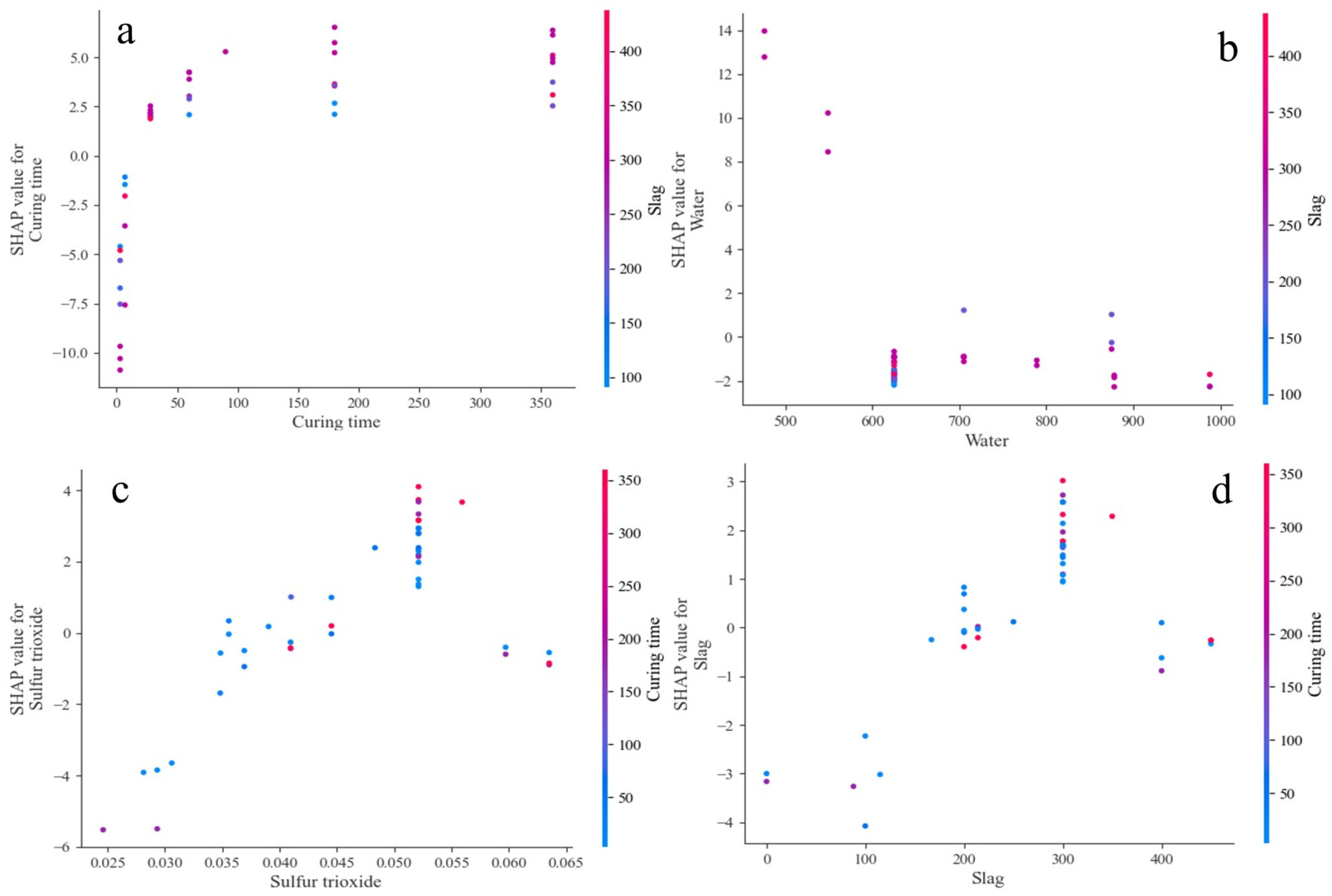
Figure 12a illustrates the influence of curing time (X13) combined with slag (X1) content on model predictions. The x-axis represents curing time, ranging from 0 to 350 days, while the y-axis represents the SHAP value reflecting the impact of curing time on model predictions. The color encoding indicates the level of slag content. At low curing times, increasing slag content generally decreases the model prediction value. In the medium curing time range, the effect is both positive and negative, depending on the slag content. At high curing times, increasing slag content tends to increase model predictions. The most significant value occurs around 250 days of curing time, with SHAP values approaching 5.0. Research shows that as curing time increases, the hydration degree of the cementitious materials becomes more complete [56], and the strength of the fill material also increases, which aligns with the trend reflected in the dependence plot.
Figure 12b shows the effect of water content combined with slag content on model predictions. As water content increases, SHAP values gradually decrease, indicating that high water content reduces the positive impact on model predictions. The most significant effect occurs when water content is around 600 g, with SHAP values close to 12.0, indicating that for a system of 500 g cementitious materials and 2000 g tailings, the water content of 600 g (water-to-cement ratio 1.2) has the most positive impact on model predictions.
Figure 12c illustrates the combined effect of sulfur trioxide (X9) content and curing time on model predictions. At low sulfur trioxide levels (<4.0%), increasing its content generally elevates model predictions, particularly under short curing durations. Within the medium sulfur trioxide range (4.0–5.1%), the effect exhibits both positive and negative influences, varying with curing time and demonstrating a complex interaction pattern. In the high sulfur trioxide range (5.1–6.5%), increased content typically reduces model predictions, especially during extended curing periods. The most significant impact occurs at approximately 5.5% sulfur trioxide content, where SHAP values approach 4.0. The increase in sulfur trioxide content induces volume expansion in the mortar, compromising the stability of strength development. As sulfur trioxide content rises, the duration of its impact on volume expansion extends, thereby reducing the fill material’s density and strength. This observation aligns with the model interpretation. Notably, within the cementitious material system, SO3 content triggers mortar volume expansion, affecting the stability of strength development. Research indicates that when SO3 content is below 5.16%, its influence on volume expansion persists for approximately 3–56 days, whereas content exceeding 5.16% extends this effect to 91 days [57]. Prolonged exposure to this expansion mechanism diminishes the compactness of the fill material and ultimately reduces its strength, consistent with the trend elucidated by the model interpretation.
Figure 12d illustrates the impact of slag content combined with curing time on model predictions. The most significant value occurs when slag content is around 300 g (approximately 60% in cementitious materials), with SHAP values approaching 2.5. At low slag content, increasing slag content typically lowers model predictions. In the medium slag content range (100–300 g), the effect is both positive and negative, depending on curing time. At high slag content, the model tends to predict higher values, especially with longer curing times. Research has shown that slag affects the final setting time and hydration degree of fill materials, but after a certain curing period, slag’s effect on compressive strength no longer changes [58]. This result aligns with the trend reflected in the model dependence plot, indicating that the model effectively captures the interaction between slag content and curing time in predicting compressive strength.
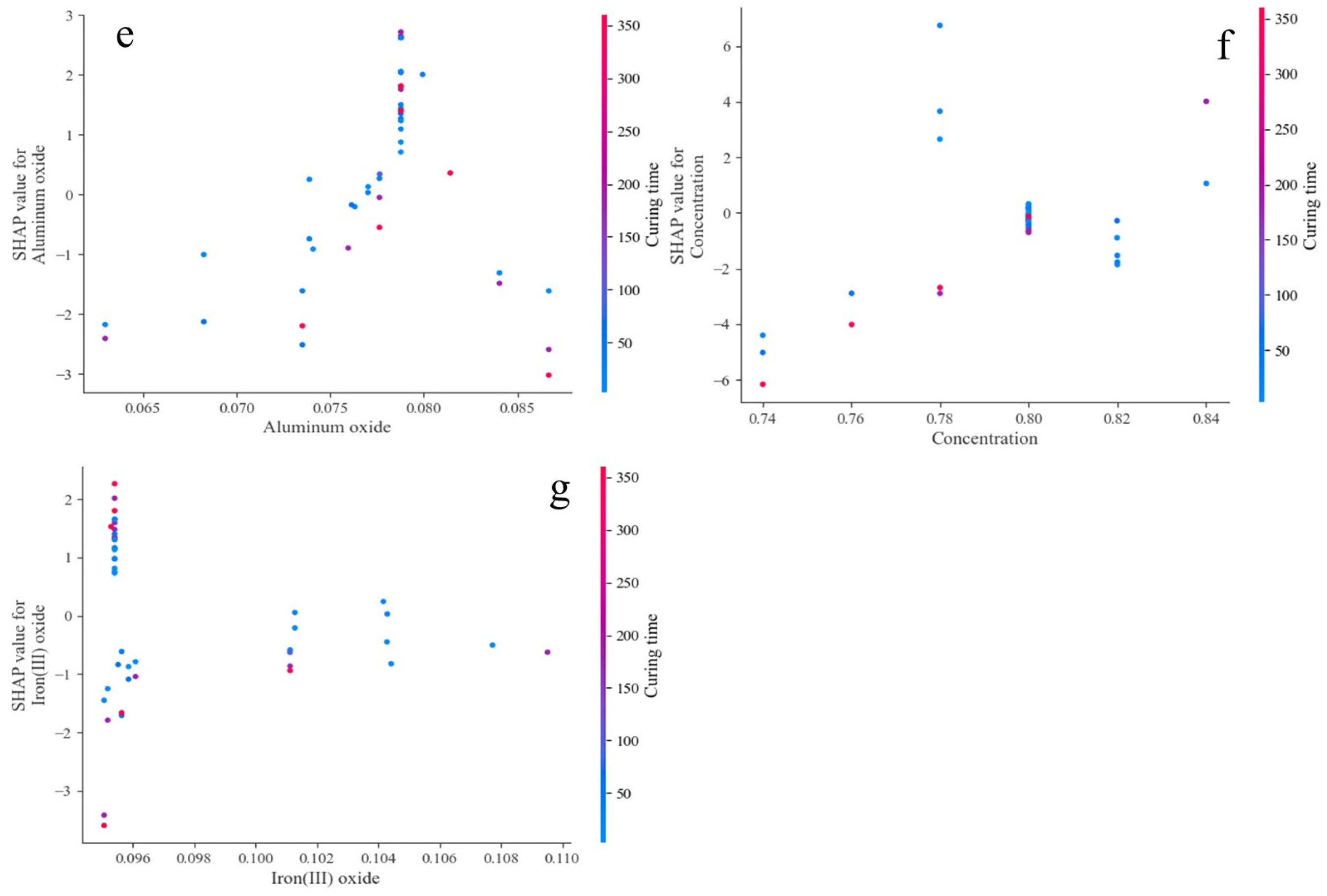
Figure 12e demonstrates the effect of aluminum oxide (X8) content combined with curing time on model predictions. At low aluminum oxide content (6.5–7.0%), increasing its content generally decreases model predictions, especially with shorter curing times. At high aluminum oxide content, the model tends to predict higher values, particularly with longer curing times. In the medium aluminum oxide content range (8.0–8.5%), the effect is both positive and negative, depending on curing time. The most significant value occurs at around 7.5% aluminum oxide content, with SHAP values close to 2.5. Research has shown that in slag-based cementitious materials, compressive strength increases with the addition of nano-aluminum oxide, but after a certain point, it decreases [59]. This trend aligns with the model’s explanation, where the influence of aluminum oxide on compressive strength becomes negative beyond 8%.
Figure 12f shows the effect of concentration (X11) combined with curing time on model predictions. At lower concentrations (0.74–0.76), increasing concentration generally lowers model predictions, especially with shorter curing times. In the medium concentration range (0.76–0.80), the effect is complex, with both positive and negative impacts. At high concentrations (0.80–0.84), increasing concentration tends to increase model predictions, especially with longer curing times. The most significant value occurs at a concentration of around 0.78, with SHAP values close to 6.0. As the concentration of the filling material increases, compressive strength increases because more particle contact points are created, providing better support and reducing internal porosity, thus improving overall density [60].
Figure 12g shows the effect of iron oxide (X7) content combined with curing time on model predictions. At low iron oxide content (10–10.4%), increasing its content significantly increases model predictions, particularly at shorter curing times. At high iron oxide content, the effect tends to reduce predictions, especially at longer curing times. In the medium iron oxide content range (10.4–11%), both positive and negative effects are observed, depending on curing time. The most significant value occurs at around 9.7% iron oxide content, with SHAP values close to 2.0.

4. Conclusions

This study developed a prediction model for the compressive strength of fly ash–slag–desulfurized gypsum-based backfill materials by employing recursive feature elimination for feature selection. A combination of multiple models and algorithms was constructed, from which the most accurate predictive model was selected and comprehensively interpreted. The following conclusions were drawn:
Among the four models, the Gradient Boosting (GB) model performed the best, and the prediction accuracy of all four models was high with a coefficient of determination (R2) greater than 0.8 after parameter tuning. Among them, the GB model optimized by Gray Wolf Optimization (GWO) showed the best performance, achieving a very high R2 of 0.9335 on the test set, while maintaining a low mean absolute error (MAE = 1.937 MPa) and mean squared error (MSE = 3.15 MPa2), demonstrating the excellent nonlinear modeling capability of the GB model.
Among the four hyperparameter tuning algorithms, GWO and Whale Optimization Algorithm (WOA) showed the best optimization effects. Compared to Bayesian Optimization (BO) and Particle Swarm Optimization (PSO), the models tuned with GWO had the lowest average error. Additionally, GWO only requires a small number of adjustable parameters and can dynamically switch between global and local search, making it more efficient than the other three algorithms in finding the global optimal solution.
SHAP value analysis of the GWO-GB model revealed that curing time was the most important feature, accounting for 27.99% of the feature importance. The impact of water had both positive and negative effects, accounting for 22.16%. Next, sulfur trioxide accounted for 18.98%, followed by slag, alumina, concentration, and iron oxide.
Based on the feature dependence graphs, the GWO-GB model revealed the dynamic interaction mechanisms between various features and compressive strength, quantitatively defining the threshold range for the positive impact of features. The maximum feature contribution was observed when the water content was 600 g (water-to-binder ratio of 1.2), with a SHAP value of 12.0; sulfur trioxide content was around 5.5%, with a SHAP value of 4.0; slag content was approximately 300 g (about 60% of the binder), with a SHAP value of 2.5; alumina content was around 7.5%, with a SHAP value of 2.5; slurry concentration was about 0.78, with a SHAP value close to 6.0; and iron oxide content was approximately 9.7%, with a SHAP value close to 2.0.
The RFE-GWO-GB model’s compressive strength prediction achieved an R2 of 0.9335. However, the mean absolute error was relatively high at 1.937 MPa, resulting in larger prediction deviations for filling materials with lower compressive strength. This is due to the database’s compressive strength data being skewed, with the average compressive strength reaching 13 MPa. Future researchers can increase data diversity and broaden the database, which will effectively improve the model’s prediction performance.

Author Contributions

Conceptualization, S.Z.; methodology, T.F.; software, T.F.; validation, T.F.; formal analysis, W.N.; investigation, W.N.; resources, W.N.; data curation, T.F.; writing—original draft preparation, T.F.; writing—review and editing, S.Z.; visualization, T.F.; supervision, W.N.; project administration, S.Z.; funding acquisition, S.Z. All authors have read and agreed to the published version of the manuscript.

Funding

This work was supported by Jing-Jin-Ji Regional Integrated Environmental Improvement-National Science and Technology Major Project (2025ZD1202700).

Institutional Review Board Statement

Not applicable.

Informed Consent Statement

Not applicable.

Data Availability Statement

The raw data supporting the conclusions of this article will be made available by the authors on request.

Acknowledgments

Thank you for the work of all participating researchers.

Conflicts of Interest

The authors declare no conflicts of interest.

References

  1. Niu, Y.; Wen, L.; Guo, X.; Hui, S. Co-disposal and reutilization of municipal solid waste and its hazardous incineration fly ash. Environ. Int. 2022, 166, 107346. [Google Scholar] [CrossRef] [PubMed]
  2. Alidoust, P.; Keramati, M.; Hamidian, P.; Amlashi, A.T.; Gharehveran, M.M.; Behnood, A. Prediction of the shear modulus of municipal solid waste (MSW): An application of machine learning techniques. J. Clean. Prod. 2021, 303, 127053. [Google Scholar] [CrossRef]
  3. Shalchian, M.M.; Arabani, M.; Farshi, M.; Ranjbar, P.Z.; Khajeh, A.; Payan, M. Sustainable Construction Materials: Application of Chitosan Biopolymer, Rice Husk Biochar, and Hemp Fibers in Geo-Structures. Case Stud. Constr. Mater. 2025, 22, e04528. [Google Scholar] [CrossRef]
  4. Jamaldar, A.; Asadi, P.; Salimi, M.; Payan, M.; Ranjbar, P.Z.; Arabani, M.; Ahmadi, H. Application of Natural and Synthetic Fibers in Bio-Based Earthen Composites: A State-of-the-Art Review. Results Eng. 2025, 25, 103732. [Google Scholar] [CrossRef]
  5. Hatefi, M.H.; Arabani, M.; Payan, M.; Ranjbar, P.Z. The Influence of Volcanic Ash (VA) on the Mechanical Properties and Freeze-Thaw Durability of Lime Kiln Dust (LKD)-Stabilized Kaolin Clayey Soil. Results Eng. 2024, 24, 103077. [Google Scholar] [CrossRef]
  6. Záleská, M.; Pavlík, Z.; Pavlíková, M.; Pivák, A.; Reiterman, P.; Lauermannová, A.-M.; Jiříčková, A.; Průša, F.; Jankovský, O. Towards immobilization of heavy metals in low-carbon composites based on magnesium potassium phosphate cement, diatomite, and fly ash from municipal solid waste. Constr. Build. Mater. 2025, 470, 140621. [Google Scholar] [CrossRef]
  7. Carmona-Ramírez, J.D.; Bedoya-Henao, C.A.; Cabrera-Poloche, F.D.; Taborda-Llano, I.; Viana-Casas, G.A.; Restrepo-Baena, O.J.; Tobón, J.I. Exploring sustainable construction: A case study on the potential of municipal solid waste incineration ashes as building materials in San Andrés island. Case Stud. Constr. Mater. 2025, 22, e04351. [Google Scholar] [CrossRef]
  8. Li, Y.; Yan, X.; Wan, M.; Fan, L.; Hu, J.; Liang, Z.; Liu, J.; Xing, F. Optimization of municipal solid waste incineration bottom ash geopolymer with granulated blast furnace slag (GGBFS): Microstructural development and heavy metal solidification mechanism. Case Stud. Constr. Mater. 2025, 22, e04423. [Google Scholar] [CrossRef]
  9. Xu, Z.; Li, C.; Xiao, B.; Chen, G. Development of slag-based filling cementitious materials and their application in ultrafine tailing sand filling. Constr. Build. Mater. 2024, 452, 17. [Google Scholar] [CrossRef]
  10. Salimi, M.; Payan, M.; Hosseinpour, I.; Arabani, M.; Ranjbar, P.Z. Effect of Glass Fiber (GF) on the Mechanical Properties and Freeze-Thaw (F-T) Durability of Lime-Nanoclay (NC)-Stabilized Marl Clayey Soil. Constr. Build. Mater. 2024, 416, 135227. [Google Scholar] [CrossRef]
  11. Mohammadi, E.L.; Najafi, E.K.; Ranjbar, P.Z.; Payan, M.; Chenari, R.J.; Fatahi, B. Recycling Industrial Alkaline Solutions for Soil Stabilization by Low-Concentrated Fly Ash-Based Alkali Cements. Constr. Build. Mater. 2023, 393, 132083. [Google Scholar] [CrossRef]
  12. Jin, L.; Chen, M.; Wang, Y.; Peng, Y.; Yao, Q.; Ding, J.; Ma, B.; Lu, S. Utilization of mechanochemically pretreated municipal solid waste incineration fly ash for supplementary cementitious material. J. Environ. Chem. Eng. 2023, 11, 109112. [Google Scholar] [CrossRef]
  13. Zamanian, M.; Salimi, M.; Payan, M.; Noorzad, A.; Hassanvandian, M. Development of High-Strength Rammed Earth Walls with Alkali-Activated Ground Granulated Blast Furnace Slag (GGBFS) and Waste Tire Textile Fiber (WTTF) as a Step towards Low-Carbon Building Materials. Constr. Build. Mater. 2023, 394, 132180. [Google Scholar] [CrossRef]
  14. Wang, Z.; Liu, H.; Zhang, Y.; Chen, Z.; Zhao, R.; Jia, Y.; Yong, M.; Li, G. Preparation and Properties of Expansive Backfill Material Based on Municipal Solid Waste Incineration Fly Ash and Coal Gangue. Minerals 2024, 14, 513. [Google Scholar] [CrossRef]
  15. Wang, K.; Li, K.; Huang, X.; Ni, W.; Zhang, S. Leaching characteristics of Cr in municipal solid waste incineration fly ash solidified/stabilized using blast furnace slag-based cementitious materials. Int. J. Environ. Sci. Technol. 2022, 19, 7457–7468. [Google Scholar] [CrossRef]
  16. Li, J.; Fu, P.; Zhang, S.; Liu, Y.; Wu, C.; Ni, W. Development of hydration potential in CFBC bottom ash activated by MSWI fly ash: Depolymerization and repolymerization during long-term reactions. Constr. Build. Mater. 2025, 489, 142219. [Google Scholar] [CrossRef]
  17. Su, L.; Wu, S.; Yu, F.; Zhu, W.; Zhang, X.; Liang, B. Utilizing municipal solid waste incineration fly ash for mine goaf filling: Preparation, optimization, and heavy metal leaching study. Environ. Res. 2025, 266, 120594. [Google Scholar] [CrossRef]
  18. Li, X.; Yu, Z.; Wu, M.B. Effect of MSWI fly ash and incineration residues on cement performances. J. Wuhan Univ. Technol.-Mater. Sci. Ed. 2010, 25, 312–315. [Google Scholar] [CrossRef]
  19. Wu, M.; Wang, C.; Zuo, Y.; Yang, S.; Zhang, J.; Luo, Y. Study on strength prediction and strength change of Phosphogypsum-based composite cementitious backfill based on BP neural network. Mater. Today Commun. 2024, 41, 110331. [Google Scholar] [CrossRef]
  20. Su, L.; Li, S.; Wu, S.; Liang, B.; Zhang, X. Preparation and heavy metal solidification mechanism of physically activated municipal solid waste incineration fly ash base geopolymer backfill. Process Saf. Environ. Prot. 2025, 201, 107522. [Google Scholar] [CrossRef]
  21. Zhang, S.; Zhao, T.; Li, Y.; Li, Z.; Li, H.; Zhang, B.; Li, J.; Li, Y.; Ni, W. The effects and solidification characteristics of municipal solid waste incineration fly ash-slag-tailing based backfill blocks in underground mine condition. Constr. Build. Mater. 2024, 420, 135508. [Google Scholar] [CrossRef]
  22. Huang, B.; Gan, M.; Ji, Z.; Fan, X.; Zhang, D.; Chen, X.; Sun, Z.; Huang, X.; Fan, Y. Recent progress on the thermal treatment and resource utilization technologies of municipal waste incineration fly ash: A review. Process Saf. Environ. Prot. 2022, 159, 547–565. [Google Scholar] [CrossRef]
  23. Lan, T.; Meng, Y.; Ju, T.; Chen, Z.; Du, Y.; Deng, Y.; Song, M.; Han, S.; Jiang, J. Synthesis and application of geopolymers from municipal waste incineration fly ash (MSWI FA) as raw ingredient—A review. Resour. Conserv. Recycl. 2022, 182, 106308. [Google Scholar] [CrossRef]
  24. Song, Z.; Xia, Y.; Zhang, Y.; Xu, M.; Wang, L.; Yan, J. Synergistic recycling of MSWI fly ash and incinerated sewage sludge ash into low-carbon binders. Constr. Build. Mater. 2024, 445, 137930. [Google Scholar] [CrossRef]
  25. Khodkari, N.; Hamidian, P.; Khodkari, H.; Payan, M.; Behnood, A. Predicting the small strain shear modulus of sands and sand-fines binary mixtures using machine learning algorithms. Transp. Geotech. 2024, 44, 101172. [Google Scholar] [CrossRef]
  26. Li, K.; Pan, K.; Xiu, W.; Li, M.; He, Z.; Wang, L. Research on Attack Detection for Traffic Signal Systems Based on Game Theory and Generative Adversarial Networks. Appl. Sci. 2024, 14, 9709. [Google Scholar] [CrossRef]
  27. Hamidian, P.; Alidoust, P.; Mohammadi Golafshani, E.; Pourrostami Niavol, K.; Behnood, A. Introduction of a novel evolutionary neural network for evaluating the compressive strength of concretes: A case of Rice Husk Ash concrete. J. Build. Eng. 2022, 61, 105293. [Google Scholar] [CrossRef]
  28. Ghanizadeh, A.R.; Abbaslou, H.; Amlashi, A.T.; Alidoust, P. Modeling of bentonite/sepiolite plastic concrete compressive strength using artificial neural network and support vector machine. Front. Struct. Civ. Eng. 2019, 13, 215–239. [Google Scholar] [CrossRef]
  29. Arachchilage, C.B.; Fan, C.; Zhao, J.; Arachchilage, C.B.; Fan, C.; Zhao, J.; Huang, G.; Liu, W.V. A machine learning model to predict unconfined compressive strength of alkali-activated slag-based cemented paste backfill. J. Rock Mech. Geotech. Eng. 2023, 15, 2803–2815. [Google Scholar] [CrossRef]
  30. Cheng, H.; Hu, J.; Hu, C.; Deng, F. Strength prediction of paste filling material based on convolutional neural network. Comput. Intell. 2021, 37, 1355–1366. [Google Scholar] [CrossRef]
  31. Qi, C.; Zheng, J.; Yang, X.; Chen, Q.; Wu, M. Application of deep neural network in the strength prediction of cemented paste backfill based on a global dataset. Constr. Build. Mater. 2023, 391, 131827. [Google Scholar] [CrossRef]
  32. Zhang, B.; Li, K.; Chen, D.; Han, B.; Hu, Y.; Liu, B. Exploration of the use of superfine tailings and ternary solid waste-based binder to prepare environmentally friendly backfilling materials: Hydration mechanisms and machine learning modeling. J. Environ. Chem. Eng. 2025, 13, 115662. [Google Scholar] [CrossRef]
  33. Hu, Y.; Ye, Y.; Zhang, B.; Li, K.; Han, B. Distribution characterization and strength prediction of backfill in underhand drift stopes based on sparrow search algorithm-extreme learning machine and field experiments. Case Stud. Constr. Mater. 2024, 21, e03784. [Google Scholar] [CrossRef]
  34. Qiu, J.; Li, J.; Xiong, X.; Zhou, K. Application of a Multi-Algorithm-Optimized CatBoost Model in Predicting the Strength of Multi-Source Solid Waste Backfilling Materials. Big Data Cogn. Comput. 2025, 9, 203. [Google Scholar] [CrossRef]
  35. Wang, K.; Xu, D.; Li, K.; Ni, W. Study on the Solidification Mechanism of Cr in Ettringite and Friedel’s Salt. Metals 2022, 12, 1697. [Google Scholar] [CrossRef]
  36. Wang, K.; Li, K.; Huang, X.; Ni, W.; Zhang, S. Preparation of backfill materials by solidifying municipal solid waste incineration fly ash with slag-based cementitious materials. Int. J. Environ. Sci. Technol. 2023, 20, 2745–2756. [Google Scholar] [CrossRef]
  37. Fan, L.; Wang, D.; Yu, H.; Gong, Z.; He, Y.; Guo, J. Application of machine learning to predict the fluoride removal capability of MgO. J. Environ. Chem. Eng. 2025, 13, 115317. [Google Scholar] [CrossRef]
  38. Liu, W.; Liu, Z.; Xiong, S.; Wang, M. Comparative prediction performance of the strength of a new type of Ti tailings cemented backfilling body using PSO-RF, SSA-RF, and WOA-RF models. Case Stud. Constr. Mater. 2024, 20, e02766. [Google Scholar] [CrossRef]
  39. Fan, L.; Yu, H.; He, Y.; Guo, J.; Min, G.; Wang, J. Optimization and interpretability analysis of machine learning methods for ZnO colloid particle size prediction. ACS Appl. Nano Mater. 2025, 8, 2682–2692. [Google Scholar] [CrossRef]
  40. Ali, T.; Onyelowe, K.C.; Mahmood, M.S.; Qureshi, M.Z.; Ben Kahla, N.; Rezzoug, A.; Deifalla, A. Advanced and hybrid machine learning techniques for predicting compressive strength in palm oil fuel ash-modified concrete with SHAP analysis. Sci. Rep. 2025, 15, 4997. [Google Scholar] [CrossRef]
  41. Liu, Y.; Yu, H.; Guan, T.; Chen, P.; Ren, B.; Guo, Z. Intelligent prediction of compressive strength of concrete based on CNN-BiLSTM-MA. Case Stud. Constr. Mater. 2025, 22, e04486. [Google Scholar] [CrossRef]
  42. Yu, Y.; Jayathilakage, R.; Liu, Y.; Hajimohammadi, A. Intelligent compressive strength prediction of sustainable rubberised concrete using an optimised interpretable deep CNN-LSTM model with attention mechanism. Appl. Soft Comput. 2025, 185, 113993. [Google Scholar] [CrossRef]
  43. Wang, S.; Xia, P.; Chen, K.; Gong, F.; Wang, H.; Wang, Q.; Zhao, Y.; Jin, W. Prediction and optimization model of sustainable concrete properties using machine learning, deep learning and swarm intelligence: A review. J. Build. Eng. 2023, 80, 108065. [Google Scholar] [CrossRef]
  44. Zulfiqar, M.; Gamage, K.A.A.; Kamran, M.; Rasheed, M.B. Hyperparameter Optimization of Bayesian Neural Network Using Bayesian Optimization and Intelligent Feature Engineering for Load Forecasting. Sensors 2022, 22, 4446. [Google Scholar] [CrossRef]
  45. Tabar, M.E.; Katlav, M.; Turk, K. Explainable ensemble algorithms with grey wolf optimization for estimation of the tensile performance of polyethylene fiber-reinforced engineered cementitious composite. Mater. Today Commun. 2025, 44, 112028. [Google Scholar] [CrossRef]
  46. Kadkhodaei, M.H.; Ghasemi, E. Interpretable real-time monitoring of short-term rockbursts in underground spaces based on microseismic activities. Sci. Rep. 2025, 14, 911. [Google Scholar] [CrossRef]
  47. Saneep, K.; Sundareswaran, K.; Nayak, P.S.R.; Puthusserry, G.V. State of charge estimation of lithium-ion batteries using PSO optimized random forest algorithm and performance analysis. J. Energy Storage 2025, 114 Pt B, 115879. [Google Scholar] [CrossRef]
  48. Khoshdel Sangdeh, M.; Salimi, M.; Hakimi Khansar, H.; Dokaneh, M.; Zanganeh Ranjbar, P.; Payan, M.; Arabani, M. Predicting the precipitated calcium carbonate and unconfined compressive strength of bio-mediated sands through robust hybrid optimization algorithms. Transp. Geotech. 2024, 46, 101235. [Google Scholar] [CrossRef]
  49. Jeon, H.; Oh, S. Hybrid-Recursive Feature Elimination for Efficient Feature Selection. Appl. Sci. 2020, 10, 3211. [Google Scholar] [CrossRef]
  50. Kumar, A.; Sen, S.; Sinha, S.; Kumar, B.; Nidhi, C. Prediction of compressive strength of concrete doped with waste plastic using machine learning-based advanced regularized regression models. Asian J. Civ. Eng. 2025, 26, 1723–1741. [Google Scholar] [CrossRef]
  51. Kaliappan, J.; Srinivasan, K.; Qaisar, S.M.; Sundararajan, K.; Chang, C.-Y.; Suganthan, C. Performance Evaluation of Regression Models for the Prediction of the COVID-19 Reproduction Rate. Front. Public Health 2021, 9, 729795. [Google Scholar] [CrossRef] [PubMed]
  52. Chu, J.; Guo, B.; Zhong, T.; Guan, Q.; Wang, Y.; Niu, D. Explainable machine learning model for predicting compressive strength of CO2-cured concrete. Case Stud. Constr. Mater. 2025, 22, e04589. [Google Scholar] [CrossRef]
  53. Silva, T.C.; Wilhelm, P.V.B.; Amancio, D.R. Machine learning and economic forecasting: The role of international trade networks. Phys. A Stat. Mech. Its Appl. 2024, 649, 129977. [Google Scholar] [CrossRef]
  54. Liu, Y.; As’Arry, A.; Hassan, M.K.; Hairuddin, A.A.; Mohamad, H. Review of the grey wolf optimization algorithm: Variants and applications. Neural Comput. Appl. 2024, 36, 10. [Google Scholar] [CrossRef]
  55. Devarajulu, V.S. AI-Driven Mission-Critical Software Optimization for Small Satellites: Integrating an Automated Testing Framework. Appl. Sci. 2024, 14. [Google Scholar]
  56. Ahmad, I.; Khan, K.A.; Ahmad, T.; Alam, M.; Bashir, M.T. Influence of accelerated curing on the compressive strength of polymer-modified concrete. Front. Struct. Civ. Eng. 2022, 16, 11. [Google Scholar] [CrossRef]
  57. Sung, C.-H.; Huang, R.; Wu, Y.-H.; Tsai, C.-J.; Lai, H.-W. Influence of sulfur trioxide on volume change and compressive strength of eco-mortar. Constr. Build. Mater. 2016, 114, 464–469. [Google Scholar] [CrossRef]
  58. Yun, C.M.; Rahman, M.R.; Phing, C.Y.W.; Chie, A.W.M.; Bakri, M.K.B. The curing times effect on the strength of ground granulated blast furnace slag (GGBFS) mortar. Constr. Build. Mater. 2020, 260, 120622. [Google Scholar] [CrossRef]
  59. Huo, W.; Zhu, Z.; Sun, H.; Gao, Q.; Zhang, J.; Wan, Y.; Zhang, C. Reaction kinetics, mechanical properties, and microstructure of nano-modified recycled concrete fine powder/slag based geopolymers. J. Clean. Prod. 2022, 372, 133715. [Google Scholar] [CrossRef]
  60. Li, Y.; Fu, J.; Yang, J.; Wang, J. Research on Slurry Flowability and Mechanical Properties of Cemented Paste Backfill: Effects of Cement-to-Tailings Mass Ratio and Mass Concentration. Materials 2024, 17, 2222. [Google Scholar] [CrossRef]
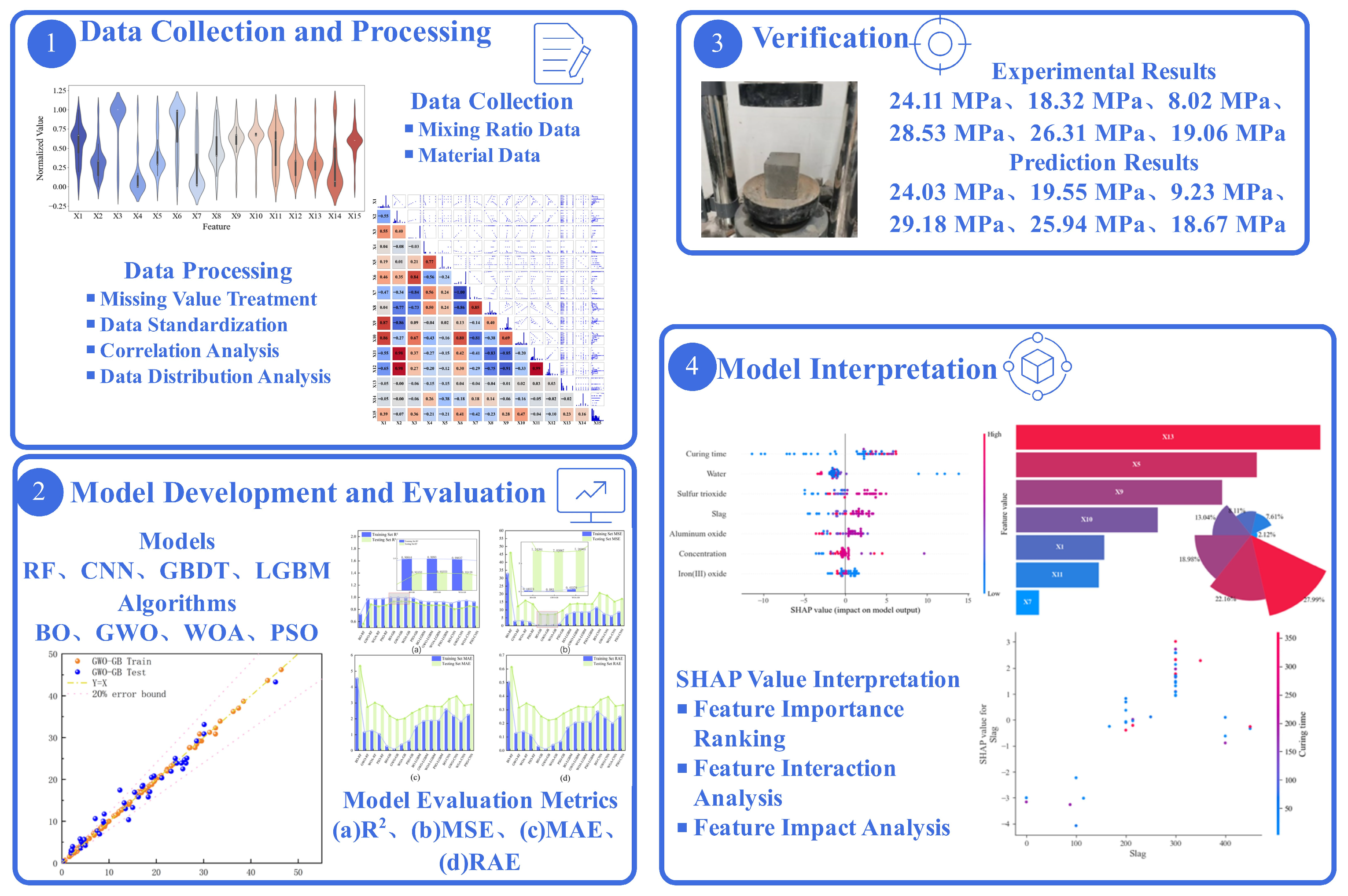
Figure 1. Research flowchart.
Applsci 15 12035 g001
Figure 2. Distribution of Normalized Feature Values Using Violin Plots.
Applsci 15 12035 g002
Figure 3. Kernel Density Estimation Plot.
Applsci 15 12035 g003
Figure 4. Evaluation of Model Performance (a) R2, (b) MSE, (c) MAE, (d) RAE.
Applsci 15 12035 g004
Figure 5. Performance Visualization: Predicted vs. Actual Values (RF Model).
Applsci 15 12035 g005
Figure 6. Performance Visualization: Predicted vs. Actual Values (CNN Model).
Applsci 15 12035 g006
Figure 7. Performance Visualization: Predicted vs. Actual Values (Gradient Boosting Model).
Applsci 15 12035 g007
Figure 8. Performance Visualization: Predicted vs. Actual Values (LightGBM Model).
Applsci 15 12035 g008
Figure 9. Scatter plots of observed versus predicted values for the WOA-GB and GWO-GB models.
Applsci 15 12035 g009
Figure 10. Validation Experiment Flowchart.
Applsci 15 12035 g010
Figure 11. Ranking of Feature Importance for Model Analysis.
Applsci 15 12035 g011
Figure 12. Feature Dependency Visualization for Gradient Boosting. (a) Curing time, (b) Water, (c) Sulfur trioxide, (d) Slag, (e) Aluminum oxide, (f) Concentration, (g) Iron(III) oxide.
Applsci 15 12035 g012aApplsci 15 12035 g012b
Table 1. XRF Composition Analysis of Raw Materials.
CompositionCaOClSiO2MgOSO3Na2OAl2O3Fe2O3K2O
fly ash39.8522.454.323.9310.285.991.592.035.96
slag40.860.0329.279.751.480.3214.761.460.46
desulfurization gypsum50.960.263.851.4740.371.370.550.1850.96
tailings16.360.0450.628.021.327.4811.542.0016.36
Table 2. Data Analysis of Feature Numbers.
FeatureFeature NameMeanMinMaxMedianStd DevQ25%Q75%
X1Slag255.690.00450.00300.00106.73200.00300.00
X2Fly ash148.430.00450.00150.0097.3768.00150.00
X3Desulfurization gypsum44.9415.0050.0050.0010.7850.0050.00
X4Tailings2247.022000.004000.002000.00518.392000.002273.00
X5Water682.03476.00987.80625.00127.47625.00705.13
X6Calcium oxide0.210.180.210.210.010.200.21
X7Iron oxide0.100.100.110.100.000.100.10
X8Silicon dioxide0.450.410.490.440.020.440.46
X9Aluminum oxide0.080.060.090.080.000.080.08
X10Sulfur trioxide0.050.020.060.050.010.040.05
X11Chlorine0.010.000.040.010.010.010.01
X12Potassium sodium oxide0.020.020.040.020.000.020.02
X13Curing time92.103.00360.0028.00118.357.00180.00
X14Concentration0.800.740.840.800.020.800.80
X15Compressive strength13.580.1146.4211.4310.804.0220.62
Table 3. Model Parameters and Feature Selection.
Optimization-Model AbbreviationParametersFeatures
RF{‘max_depth’: None (5–30), ‘n_estimators’: 100 (50–500), ‘min_samples_split’: 2 (2–20), ‘min_samples_leaf’: 1 (1–10)}[‘Slag’, ‘Fly ash’, ‘Desulfurization gypsum’, ‘Tailings’, ‘Water’, ‘Calcium oxide’, ‘Iron(III) oxide’, ‘Silicon dioxide’, ‘Aluminum oxide’, ‘Sulfur trioxide’, ‘Chlorine’, ‘Potassium sodium oxide’, ‘Curing time’, ‘Concentration’]
GBDT{‘max_depth’: 3 (3–10), ‘n_estimators’: 100 (50–500), ‘min_samples_split’: 2 (2–20), ‘min_samples_leaf’: 1 (1–10), ‘learning_rate’: 0.1 (0.01–0.3)}[‘Slag’, ‘Fly ash’, ‘Desulfurization gypsum’, ‘Tailings’, ‘Water’, ‘Calcium oxide’, ‘Iron(III) oxide’, ‘Silicon dioxide’, ‘Aluminum oxide’, ‘Sulfur trioxide’, ‘Chlorine’, ‘Potassium sodium oxide’, ‘Curing time’, ‘Concentration’]
LGBM{‘num_leaves’: 31 (10–128), ‘max_depth’: 6 (5–30), ‘n_estimators’: 100 (50–500), ‘learning_rate’: 0.1 (0.01–0.3), ‘min_child_samples’: 20 (1–50)}[‘Slag’, ‘Fly ash’, ‘Desulfurization gypsum’, ‘Tailings’, ‘Water’, ‘Calcium oxide’, ‘Iron(III) oxide’, ‘Silicon dioxide’, ‘Aluminum oxide’, ‘Sulfur trioxide’, ‘Chlorine’, ‘Potassium sodium oxide’, ‘Curing time’, ‘Concentration’]
CNN{‘filters1′: 32 (16–128), ‘filters2′: 32 (16–128), ‘kernel_size’: 3 (2–5), ‘dense_units’: 64 (32–128), ‘dropout_rate’: 0.2 (0.1–0.5), ‘learning_rate’: 0.001 (0.0001–0.01)}[‘Slag’, ‘Fly ash’, ‘Desulfurization gypsum’, ‘Tailings’, ‘Water’, ‘Calcium oxide’, ‘Iron(III) oxide’, ‘Silicon dioxide’, ‘Aluminum oxide’, ‘Sulfur trioxide’, ‘Chlorine’, ‘Potassium sodium oxide’, ‘Curing time’, ‘Concentration’]
GS-RF{‘max_depth’: 10 (5–30), ‘n_estimators’: 100 (50–500), ‘min_samples_split’: 2 (2–20), ‘min_samples_leaf’: 1 (1–10)}[‘Slag’, ‘Fly ash’, ‘Desulfurization gypsum’, ‘Tailings’, ‘Water’, ‘Calcium oxide’, ‘Iron(III) oxide’, ‘Silicon dioxide’, ‘Aluminum oxide’, ‘Sulfur trioxide’, ‘Chlorine’, ‘Potassium sodium oxide’, ‘Curing time’, ‘Concentration’]
GS-GB{‘max_depth’: 3 (3–10), ‘n_estimators’: 100 (50–500), ‘learning_rate’: 0.1 (0.01–0.3), ‘min_samples_split’: 2 (2–20), ‘min_samples_leaf’: 1 (1–10)}[‘Slag’, ‘Fly ash’, ‘Desulfurization gypsum’, ‘Tailings’, ‘Water’, ‘Calcium oxide’, ‘Iron(III) oxide’, ‘Silicon dioxide’, ‘Aluminum oxide’, ‘Sulfur trioxide’, ‘Chlorine’, ‘Potassium sodium oxide’, ‘Curing time’, ‘Concentration’]
GS-LGBM{‘max_depth’: −1 (5–30), ‘n_estimators’: 100 (50–1000), ‘learning_rate’: 0.1 (0.01–0.3), ‘num_leaves’: 31 (10–128), ‘min_child_samples’: 20 (1–50)}[‘Slag’, ‘Fly ash’, ‘Desulfurization gypsum’, ‘Tailings’, ‘Water’, ‘Calcium oxide’, ‘Iron(III) oxide’, ‘Silicon dioxide’, ‘Aluminum oxide’, ‘Sulfur trioxide’, ‘Chlorine’, ‘Potassium sodium oxide’, ‘Curing time’, ‘Concentration’]
RFE-BO-RF{‘max_depth’: 10 (5–30), ‘min_samples_leaf’: 1 (1–10), ‘min_samples_split’: 6 (2–20), ‘n_estimators’: 94 (100–1000)}[‘Slag’, ‘Water’, ‘Calcium oxide’, ‘Iron(III) oxide’, ‘Silicon dioxide’, ‘Aluminum oxide’, ‘Sulfur trioxide’, ‘Chlorine’, ‘Curing time’, ‘Concentration’]
RFE-GWO-RF{‘max_depth’: 5 (5–30), ‘min_samples_leaf’: 9 (1–10), ‘min_samples_split’: 6 (2–20), ‘n_estimators’: 158 (100–1000)}[‘Slag’, ‘Water’, ‘Calcium oxide’, ‘Iron(III) oxide’, ‘Silicon dioxide’, ‘Aluminum oxide’, ‘Sulfur trioxide’, ‘Chlorine’, ‘Curing time’, ‘Concentration’]
RFE-WOA-RF{‘max_depth’: 5 (5–30), ‘min_samples_leaf’: 7 (1–10), ‘min_samples_split’: 2 (2–20), ‘n_estimators’: 65 (100–1000)}[‘Slag’, ‘Water’, ‘Calcium oxide’, ‘Iron(III) oxide’, ‘Silicon dioxide’, ‘Aluminum oxide’, ‘Sulfur trioxide’, ‘Chlorine’, ‘Curing time’, ‘Concentration’]
RFE-PSO-RF{‘max_depth’: 8 (5–30), ‘min_samples_leaf’: 1 (1–10), ‘min_samples_split’: 5 (2–20), ‘n_estimators’: 101 (100–1000)}[‘Slag’, ‘Water’, ‘Calcium oxide’, ‘Iron(III) oxide’, ‘Silicon dioxide’, ‘Aluminum oxide’, ‘Sulfur trioxide’, ‘Chlorine’, ‘Curing time’, ‘Concentration’]
RFE-BO-GB{‘max_depth’: 4 (5–30), ‘learning_rate’: 0.17817087100112233 (0.01–0.3), ‘min_samples_leaf’: 9 (1–10), ‘min_samples_split’: 18 (2–20), ‘n_estimators’: 148 (100–1000)}[‘Slag’, ‘Water’, ‘Iron(III) oxide’, ‘Aluminum oxide’, ‘Sulfur trioxide’, ‘Curing time’, ‘Concentration’]
RFE-GWO-GB{‘max_depth’: 5 (5–30), ‘learning_rate’: 0.17028188992197366 (0.01–0.3), ‘min_samples_leaf’: 4 (1–10), ‘min_samples_split’: 4 (2–20), ‘n_estimators’: 101 (100–1000)}[‘Slag’, ‘Water’, ‘Iron(III) oxide’, ‘Aluminum oxide’, ‘Sulfur trioxide’, ‘Curing time’, ‘Concentration’]
RFE-WOA-GB{‘max_depth’: 8 (5–30), ‘learning_rate’: 0.10333208140151896 (0.01–0.3), ‘min_samples_leaf’: 1 (1–10), ‘min_samples_split’: 15 (2–20), ‘n_estimators’: 128 (100–1000)}[‘Slag’, ‘Water’, ‘Iron(III) oxide’, ‘Aluminum oxide’, ‘Sulfur trioxide’, ‘Curing time’, ‘Concentration’]
RFE-PSO-GB{‘max_depth’: 7 (5–30), ‘learning_rate’: 0.18642056953682531 (0.01–0.3), ‘min_samples_leaf’: 3 (1–10), ‘min_samples_split’: 3 (2–20), ‘n_estimators’: 64 (100–1000)}[‘Slag’, ‘Water’, ‘Iron(III) oxide’, ‘Aluminum oxide’, ‘Sulfur trioxide’, ‘Curing time’, ‘Concentration’]
RFE-BO-LGBM{‘max_depth’: 7 (5–30), ‘learning_rate’: 0.2 (0.01–0.3), ‘min_samples_leaf’: 7 (1–10), ‘min_samples_split’: 16 (2–20), ‘n_estimators’: 143 (100–1000)}[‘Slag’, ‘Fly ash’, ‘Tailings’, ‘Water’, ‘Calcium oxide’, ‘Aluminum oxide’, ‘Sulfur trioxide’, ‘Chlorine’, ‘Potassium sodium oxide’, ‘Curing time’]
RFE-GWO-LGBM{‘max_depth’: 8 (5–30), ‘learning_rate’: 0.031555063806171034 (0.01–0.3), ‘min_samples_leaf’: 8 (1–10), ‘min_samples_split’: 19 (2–20), ‘n_estimators’: 50 (100–1000)}[‘Slag’, ‘Fly ash’, ‘Tailings’, ‘Water’, ‘Calcium oxide’, ‘Aluminum oxide’, ‘Sulfur trioxide’, ‘Chlorine’, ‘Potassium sodium oxide’, ‘Curing time’]
RFE-WOA-LGBM{‘max_depth’: 5 (5–30), ‘learning_rate’: 0.17537439537639113 (0.01–0.3), ‘min_samples_leaf’: 8 (1–10), ‘min_samples_split’: 12 (2–20), ‘n_estimators’: 87 (100–1000)}[‘Slag’, ‘Fly ash’, ‘Tailings’, ‘Water’, ‘Calcium oxide’, ‘Aluminum oxide’, ‘Sulfur trioxide’, ‘Chlorine’, ‘Potassium sodium oxide’, ‘Curing time’]
RFE-PSO-LGBM{‘max_depth’: 4 (5–30), ‘learning_rate’: 0.14414451841810513 (0.01–0.3), ‘min_samples_leaf’: 4 (1–10), ‘min_samples_split’: 2 (2–20), ‘n_estimators’: 172 (100–1000)}[‘Slag’, ‘Fly ash’, ‘Tailings’, ‘Water’, ‘Calcium oxide’, ‘Aluminum oxide’, ‘Sulfur trioxide’, ‘Chlorine’, ‘Potassium sodium oxide’, ‘Curing time’]
RFE-BO-CNN{‘learning_rate’: 0.005577 (0.0001–0.1), ‘batch_size’: 30 (16–256), ‘epochs’: 98, ‘filters1′: 50 (16–256), ‘kernel_size’: 4 (3–7), ‘filters2′: 65, ‘dense_units’: 109 (64–512), ‘validation_MSE’: 9.3207}[‘Slag’, ‘Fly ash’, ‘Desulfurization gypsum’, ‘Tailings’, ‘Water’, ‘Iron(III) oxide’, ‘Aluminum oxide’, ‘Sulfur trioxide’, ‘Curing stime’, ‘Concentration’]
RFE-GWO-CNN{‘learning_rate’: 0.009306 (0.0001–0.1), ‘batch_size’: 33 (16–256), ‘epochs’: 37, ‘filters1′: 96 (16–256), ‘kernel_size’: 5 (3–7), ‘filters2′: 28, ‘dense_units’: 171 (64–512), ‘validation_MSE’: 22.4184}[‘Slag’, ‘Fly ash’, ‘Desulfurization gypsum’, ‘Tailings’, ‘Water’, ‘Iron(III) oxide’, ‘Aluminum oxide’, ‘Sulfur trioxide’, ‘Curing time’, ‘Concentration’]
RFE-WOA-CNN{‘learning_rate’: 0.009197 (0.0001–0.1), ‘batch_size’: 109 (16–256), ‘epochs’: 98, ‘filters1′: 126 (16–256), ‘kernel_size’: 5 (3–7), ‘filters2′: 126, ‘dense_units’: 251 (64–512), ‘validation_MSE’: 26.3298}[‘Slag’, ‘Fly ash’, ‘Desulfurization gypsum’, ‘Tailings’, ‘Water’, ‘Iron(III) oxide’, ‘Aluminum oxide’, ‘Sulfur trioxide’, ‘Curing time’, ‘Concentration’]
RFE-PSO-CNN{‘learning_rate’: 0.005293 (0.0001–0.1), ‘batch_size’: 20 (16–256), ‘epochs’: 31, ‘filters1′: 109 (16–256), ‘kernel_size’: 4 (3–7), ‘filters2′: 65, ‘dense_units’: 131 (64–512), ‘validation_MSE’: 18.7533}[‘Slag’, ‘Fly ash’, ‘Desulfurization gypsum’, ‘Tailings’, ‘Water’, ‘Iron(III) oxide’, ‘Aluminum oxide’, ‘Sulfur trioxide’, ‘Curing time’, ‘Concentration’]
Table 4. Summary of Average Errors by Model.
Model-Algorithm CombinationTraining Set R2Training Set MAETraining Set MSETraining Set RAETesting Set R2Testing Set MAETesting Set MSETesting Set RAE
RF0.866 ± 0.0032.765 ± 0.08216.098 ± 0.4560.307 ± 0.0050.824 ± 0.0043.236 ± 0.10118.662 ± 0.5820.373 ± 0.006
GB0.869 ± 0.0022.550 ± 0.06815.540 ± 0.3890.284 ± 0.0040.863 ± 0.0032.798 ± 0.08914.484 ± 0.4980.323 ± 0.005
LGBM0.759 ± 0.0054.061 ± 0.12530.037 ± 0.8720.450 ± 0.0070.668 ± 0.0064.355 ± 0.14235.156 ± 1.0380.502 ± 0.008
CNN0.493 ± 0.0076.468 ± 0.18360.666 ± 1.6210.725 ± 0.0090.335 ± 0.0086.607 ± 0.19470.302 ± 1.7450.762 ± 0.010
GS-RF0.867 ± 0.0022.773 ± 0.07916.064 ± 0.4210.308 ± 0.0040.823 ± 0.0033.252 ± 0.09718.708 ± 0.5510.375 ± 0.005
GS-GB0.869 ± 0.0022.550 ± 0.06715.540 ± 0.3850.284 ± 0.0040.863 ± 0.0032.798 ± 0.08814.484 ± 0.4950.323 ± 0.005
GS-LGBM0.759 ± 0.0054.061 ± 0.12330.037 ± 0.8650.450 ± 0.0070.668 ± 0.0064.355 ± 0.14035.156 ± 1.0300.502 ± 0.008
GS-CNN0.517 ± 0.0066.177 ± 0.16757.455 ± 1.5120.690 ± 0.0080.465 ± 0.0075.944 ± 0.17656.573 ± 1.6380.685 ± 0.009
RFE-BO-RF0.724 ± 0.0044.569 ± 0.13132.976 ± 0.9130.506 ± 0.0060.564 ± 0.0055.333 ± 0.14446.078 ± 1.2810.615 ± 0.007
RFE-GWO-RF0.975 ± 0.0011.173 ± 0.0212.998 ± 0.0580.130 ± 0.0020.884 ± 0.0022.747 ± 0.04812.288 ± 0.1320.317 ± 0.003
RFE-WOA-RF0.972 ± 0.0011.276 ± 0.0243.306 ± 0.0640.141 ± 0.0020.849 ± 0.0033.017 ± 0.05215.925 ± 0.1450.348 ± 0.003
RFE-PSO-RF0.979 ± 0.0011.052 ± 0.0182.479 ± 0.0490.116 ± 0.0020.871 ± 0.0022.794 ± 0.04213.663 ± 0.1210.322 ± 0.003
RFE-BO-GB0.998 ± 0.0000.293 ± 0.0030.186 ± 0.0010.032 ± 0.0000.932 ± 0.0012.180 ± 0.0317.243 ± 0.0860.251 ± 0.001
RFE-GWO-GB0.999 ± 0.0000.088 ± 0.0010.083 ± 0.0000.010 ± 0.0000.934 ± 0.0011.937 ± 0.0287.031 ± 0.0770.223 ± 0.001
RFE-WOA-GB0.996 ± 0.0000.392 ± 0.0040.434 ± 0.0020.043 ± 0.0000.931 ± 0.0012.023 ± 0.0307.269 ± 0.0800.233 ± 0.001
RFE-PSO-GB0.990 ± 0.0000.620 ± 0.0051.242 ± 0.0030.069 ± 0.0000.909 ± 0.0012.368 ± 0.0379.646 ± 0.0980.273 ± 0.001
RFE-BO-LGBM0.940 ± 0.0011.554 ± 0.0227.194 ± 0.0590.172 ± 0.0020.871 ± 0.0022.604 ± 0.03513.606 ± 0.0960.300 ± 0.002
RFE-GWO-LGBM0.928 ± 0.0011.875 ± 0.0268.625 ± 0.0680.207 ± 0.0020.868 ± 0.0022.827 ± 0.03913.980 ± 0.0990.326 ± 0.002
RFE-WOA-LGBM0.927 ± 0.0011.902 ± 0.0278.692 ± 0.0700.210 ± 0.0020.870 ± 0.0022.776 ± 0.03813.783 ± 0.0980.320 ± 0.002
RFE-PSO-LGBM0.927 ± 0.0011.902 ± 0.0278.692 ± 0.0700.210 ± 0.0020.870 ± 0.0022.776 ± 0.03813.783 ± 0.0980.320 ± 0.002
RFE-BO-CNN0.902 ± 0.0012.621 ± 0.04111.661 ± 0.1090.290 ± 0.0030.804 ± 0.0033.250 ± 0.05320.683 ± 0.1410.375 ± 0.004
RFE-GWO-CNN0.937 ± 0.0012.200 ± 0.0327.584 ± 0.0880.244 ± 0.0020.820 ± 0.0033.428 ± 0.04619.072 ± 0.1260.395 ± 0.003
RFE-WOA-CNN0.949 ± 0.0011.826 ± 0.0286.115 ± 0.0760.202 ± 0.0020.856 ± 0.0032.842 ± 0.04015.220 ± 0.1110.328 ± 0.003
RFE-PSO-CNN0.926 ± 0.0012.274 ± 0.0368.803 ± 0.0970.252 ± 0.0020.839 ± 0.0032.903 ± 0.04316.990 ± 0.1290.335 ± 0.003
Disclaimer/Publisher’s Note: The statements, opinions and data contained in all publications are solely those of the individual author(s) and contributor(s) and not of MDPI and/or the editor(s). MDPI and/or the editor(s) disclaim responsibility for any injury to people or property resulting from any ideas, methods, instructions or products referred to in the content.