Abstract
Current ground investigation practice in geotechnical engineering is highly energy- and time-intensive, which is environmentally unfriendly. Several weeks are usually required to perform the investigation, and along this process, acquiring just one parameter of a soil sample may consume more than 100 Wh. Addressing this challenge, this study aimed at reducing energy consumption of ground investigation following Green AI concept, and an AI model for subsurface data prediction, which was optimized with greedy algorithm, was therefore developed. This model inputs soil parameters obtained by low-energy methods and outputs soil parameters (i.e., shear strength parameters) obtained by high-energy methods in traditional ground investigation practice. The model was established using ensemble learning techniques and a large dataset with fifteen types of parameters, which was obtained from 924 samples via a series of laboratory tests in a traditional ground investigation. Meanwhile, considering the variability on ensemble model architecture, greedy algorithm was adopted to optimize the architecture from a pool of nine base learners and six ensemble strategies. Thereby, the best-performing AI model was eventually identified, and it achieved a R2 value of 0.881 over the testing dataset, which accounts for 30% of the overall parameter dataset. With this model, the energy consumption needed to acquire the subsurface data was significantly reduced by 71%. The findings of this study pave the way for a lower-carbon but more intelligent ground investigation.
1. Introduction
Subsurface data, typically the basic soil parameters, serve as the foundational basis for the design and safety assessment of geotechnical engineering projects, including foundation optimization [1], slope stability analysis [2], and many others [3]. In traditional ground investigation workflow, soil samples are first extracted from the target site. Afterwards, laboratory tests are performed on the samples to estimate the key soil parameters, such as sieving test [4], direct shear test [5], triaxial shear test [6], and permeability test [7]. However, a critical limitation of this traditional workflow lies in its high carbon footprint, driven by the significant time and energy consumption of laboratory testing. For instance, characterizing clayey soil samples often requires continuous operation of testing equipment for several days to complete sample consolidation and shearing processes [8], and each hour of machine runtime contributes to direct energy consumption [9]. In the meantime, soil parameters commonly exhibit a remarkable variability, with correlations to the density [10], water content [11], fabric [12], particle shape [13], particle size distribution [14], and many other factors [15]. To ensure the reliability of subsurface data acquisition, extensive on-site sampling and repetitive laboratory tests have to be conducted, which not only prolongs the duration of ground investigation but also further increases energy consumption [16]. Therefore, traditional ground investigation workflow is becoming incompatible with global decarbonization goals.
As a complementary alternative to laboratory tests, in-situ tests, such as standard penetration test (SPT) and cone penetration test (CPT), are also widely implemented in traditional ground investigation workflow. Soil parameters, typically the friction angle and cohesion, can be subsequently derived from the interpretations of measured results (e.g., SPT N-value [17], cone tip resistance [18], and sleeve friction [19]). These tests originally aim at enhancing the efficiency of ground investigation, and inadvertently align with the decarbonization goal, since the needs for soil sampling and laboratory testing are eliminated and the energy consumption can be reduced [20]. However, the types of measured results from in-situ tests are few. For instance, the SPT test provides only the N-value. Consequently, the accuracy of soil parameter prediction is usually low, creating a demand for more robust prediction methods for soil parameters.
Addressing the above limitation of in-situ test, a growing number of research works delving into developing the Artificial Intelligence (AI) models for soil parameter prediction, as summarized in Table 1. These models can connect more inputs to the output soil parameters, thereby enhancing the predictive accuracy. On the one hand, researchers have targeted at the prediction of a broad spectrum of soil parameters, including soil compatibility [21,22], pH value [23,24], thermal conductivity [25,26], hydraulic conductivity [27], liquefaction susceptibility [28], moisture content [29], strength parameters (i.e., friction angle and cohesion) [30], and many others [31]. On the other hand, researchers have focused on evaluating the effectiveness of different AI models in soil strength parameter prediction. For instance, Das and Basudhar [32] have reported the effectiveness and robustness of artificial neural network (ANN) in predicting residual friction angle of clay. Random forest (RF) and supporting vector machine (SVM) have been validated to yield satisfactory performances by Pham and his coworkers [33,34]. Zhu et al. further compared the BPNN, PLSR, and SVR models and reported that the SVR model produced the best performance, especially in predicting internal friction angle [35]. In the following texts, the term “AI model” here uniformly refers to the model that teaches the machine to predict soil parameters (e.g., soil strength parameters) from other kinds of basic soil parameters.

Table 1.
AI model performance on soil parameter prediction in the literature.
Considering that the types of AI models are highly diverse, some studies concentrated on establishing universal soil databases to provide a fundamental basis for comparing the performances of different models. The soil database by Li et al. [37] was collected from 0 to 2 m depth in Singapore, containing both saturated and unsaturated hydraulic and mechanical properties. Chow et al. [38] focused on the database of clayey soils. Hengl et al. [39] further provided a worldwide database at 1 km resolution, but limited to surface soils. Besides the soil database, other works attempted to integrate the advantages of different AI models leveraging the ensemble learning technique to further improve predictive accuracy. Three ensemble strategies, i.e., bagging, voting, and stacking, have been proposed for such integration. Zhang et al. [40] have reported the effectiveness in applying ensemble learning to predict soil strength parameters. Cao et al. [41] developed an advanced meta-learner for the stacking strategy and the prediction accuracy could be further enhanced. Beyond ground investigation, the efficacy of ensemble learning has also been validated in other geotechnical applications, such as slope stability analysis [42,43] and 3D geological modeling [44]. Collectively, these works demonstrated that the ensemble model outperforms the single standalone models. However, Rabbani et al. [45] established and compared five ensemble models based on a dataset of 249 soil samples, and afterwards pointed out that the prediction accuracy varies with the model architecture significantly. Therefore, there is an urgent need to develop approaches for optimizing the architecture of ensemble models to enhance the predictive accuracy of soil parameters.
Among the aforementioned studies, the output soil parameters of AI models for ground investigation were typically based on their scientific value rather than the goal of energy efficiency (i.e., their engineering need). Additionally, these works exhibit significant variability in model architectures and performance, with no clear optimization guidelines provided to produce superior performance under equivalent energy consumption. Therefore, it is criticized that these models were not fully green from both of these perspectives. Addressing these research gaps and regarding the existing achievements in the literature, it is hypothesized that the AI model for subsurface data, which is established with ensemble learning and Green AI concept, can reduce the energy consumption of ground investigation over 50% and while preserving the predictive accuracy. Note that Green AI is defined as optimizing AI computing process or model for energy efficiency, which was primarily proposed by Schwartz [46] in 2020, and an increasing number of associated works have been published to make AI models more environmentally friendly [36]. Following this concept, the energy reduction in ground investigation can be achieved through the following two key pathways: first, the exemption of acquiring some soil parameters by tests, and second, the enhanced efficiency of AI model computation. In the subsequent sections, the output parameters of the model were first determined, based on the energy consumption associated with acquiring each parameter in traditional ground investigation workflow. Then, the model architecture is established using ensemble learning, and the architecture is optimized to reach the model greenness using the greedy algorithm (to be introduced later). Finally, the optimization and energy-saving efficacy of the model will be validated. It is anticipated that the findings of this study will lay the groundwork for more intelligent, lower-carbon ground investigation practices.
2. Dataset Obtained from Traditional Ground Investigation
2.1. Soil Parameters in Dataset
The dataset of soil parameters was collected from the ground investigation in the project of Huangpu Tram Line 2, Guangzhou. The project details can be seen in our previous work [47]. The workflow of ground investigation in this project is illustrated in Figure 1. First, boreholes were drilled to take more than 308 sets of soil samples at different horizontal positions and depths (1.5~20 m) out from the ground (see the leftmost in Figure 1). Soils from one of the boreholes are shown in the middle of Figure 1. Various types of soils (e.g., fills, clayey soils, sandy soils, granitic residual soil, and completely decomposed granite soil) were identified, which are frequently encountered in South China [48]. A series of laboratory tests were then performed on the soil samples, including sieving test, water content test, liquid-plastic limit combined test, specific gravity test, oedometer test, and direct shear test, as indicated by the rightmost in Figure 1. In this context, each sample set contained at least 3 samples to fully undergo these tests, and there were essentially more than 924 samples tested in total.
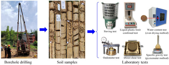
Figure 1.
Workflow of the ground investigation.
From the sieving test, six parameters (i.e., the proportions of gravel, coarse sand, medium sand, fine sand, silt, and clay) were provided. Note that the proportion of clay is equal to one minus the former five ones, and it was therefore not used in the AI model here to avoid linear correlation among parameters [49]. Another eight parameters were further obtained, including the water content, dry density, specific gravity, void ratio, liquid limit, plastic limit, compression modulus, consolidation coefficient. Finally, from direct shear tests at a constant speed of 0.8 mm/min and vertical stress varying from 100 to 400 kPa, two strength parameters (i.e., friction angle and cohesion) were also obtained for each set of soil samples.
A total of fifteen soil parameters were obtained from the ground investigation, as summarized in Table 2. As 308 sets of samples were tested, there were more than 4620 data points in the database, which is much greater than those provided in the literature [37,45]. Key statistical features for each parameter are further presented, including value range (i.e., maximum and minimum values), mean, median, and standard deviation. For most parameters, the value ranges exhibit notable breadth, with the maximum value several times greater than the minimum value. This is attributed to significant diversity in soil types at the study site, which indicates the potential generalization ability of our model here. However, one exception is the specific gravity, whose value range remains narrow (2.60–2.75). Nevertheless, this study did not focus on the optimization of the input parameters. As further observed from Table 2, the median values are close to the mean values, indicating moderate skewness in each parameter. Additionally, standard deviations reveal that the dispersion degree of all parameters is similarly moderate. Collectively, these statistical features demonstrate that the dataset exhibits high quality and strong suitability for training our AI model here. Note that though our model was established using the dataset only from the project of Huangpu Tram Line 2, its transferability to a new site will be discussed later.
Table 2.
Statistical features of the dataset.
2.2. Energy Consumption Comparison Among Soil Parameters
Different devices were employed in the aforementioned tests. Accordingly, the energy consumption to acquire the associated parameter varies significantly. Table 3 further summarizes the power ratings of used devices here. All the devices were purchased from Jingyi Instrument Co., Ltd., Shanghai, China. To enable comparison across the tests, the device operation times were further estimated on a clay sample. This soil type was selected because it requires the longest testing duration relative to other soil classes, ensuring conservative and representative time-based energy calculations. Additionally, the numbers of samples and parameters, which can be processed simultaneously in each kind of test, were determined based on the inherent parallel testing capacity of the device. Using these foundational data (device power, operation time, and simultaneous testing capacity), the energy consumption rate (i.e., the energy consumption per parameter and per sample) was determined. Note that this study focused on energy consumptions from the aspect of laboratory testing, since they are measurable from the used devices. For those indirect field costs (e.g., borehole drilling), it will be included in the future study to provide a more compressive estimation on the energy saving.
Table 3.
Energy consumption per parameter.
As presented in Table 3, the activity of consolidation test requires only 0 W, since it is conducted purely through manual operations, without any electrical device used; that is, the energy consumption of human activity is not accounted here. In both the water content test and specific gravity test, though the used oven has the highest power rating of 500 W, its capacity enables 200 samples to be cured and tested simultaneously. Consequently, the energy rates for these two tests are not the highest. Unexpectedly, the direct shear test exhibits the greatest energy consumption rate, reaching 100 Wh per parameter and per sample, which is consistent with the fact that shear strength measurement inherently involves complex mechanical processes. It is supposed that if triaxial shear test is used, energy consumption will be further increased.
2.3. Determination of Model Inputs and Outputs
Based on the above analysis, to establish the Green AI model for substrata data prediction, the first 13 parameters (i.e., X1–X13) in Table 2 should be selected as the inputs to predict the last 2 strength parameters (i.e., Y1–Y2). Prior to the model establishment, the inputs were preprocessed. Each parameter was normalized using the Z-score method to enhance the generalization of the model, since the parameter distributions were close Gaussian distributions, according to Table 2 [50]. In the meantime, the samples, which did not have complete parameter list (i.e., fifteen parameters), were removed from the database. Thereby, there are no vacancy values for the inputs, when training the model.
The Spearman correlation coefficient between each two parameters was estimated, according to Equation (1).
where ρij is the Spearman correlation coefficient between the parameters Xi and Xj; n is the number of data points; and the overline indicates the mean of the parameter. The results are then visualized as a heatmap in Figure 2. The color and the number of stars in the cell were used to indicate the correlation between two parameters. As seen in Figure 2, most cells exhibit light colors. There are 78 cells above the diagonal in total and 56 of them (accounting for ~72%) exhibit a correlation coefficient less than 0.5. Such a result indicates that X1–X13 are largely independent of each other to avoid multicollinearity in model inputs [51]. Still, some parameters are inherently and closely correlated to each other with a correlation coefficient greater than 0.8, such as X5 (liquid limit) and X6 (plastic limit). Yet, these strong correlations did not significantly affect the training of AI model, and therefore, the input optimization was not considered here. The Spearman correlation between X1–X13 and Y1–Y2 was further measured, again using Equation (1) and again shown in Figure 2. Lines with notable color intensity and thickness dominate the plot. Eight of thirteen inputs show strong positive/negative correlations (|ρ| > 0.4) with the outputs. This demonstrates strong and reliable relationships between the input candidates and the target strength parameters. Collectively, these observations validate that X1–X13 are well suited as input features for the Green AI model to predict Y1–Y2.
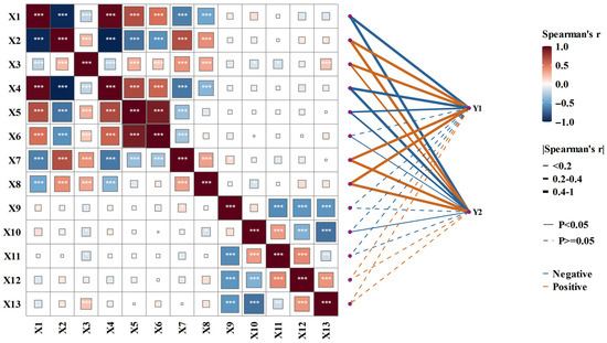
Figure 2.
Heatmap among X1–X13 and Spearman correlation to Y1–Y2.
3. Green AI Model Optimized with Greedy Algorithm
3.1. General Model Architecture
As illustrated in Figure 3, the architecture of AI model for subsurface data prediction was generally regulated by the ensemble learning technique, since as aforementioned, this technique can integrate strengths of diverse AI models. The model was powered by the dataset derived from traditional ground investigation in Section 2. The input parameters were X1–X13 in Table 2, while the output parameters were Y1–Y2 for saving energy in ground investigation. The data were further partitioned into the training data and testing data, which accounted for 70% and 30%, respectively, following the common practices in the literature [52].
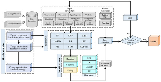
Figure 3.
Architecture of AI model for subsurface data prediction.
The architecture comprises the following two key components: base learners and an ensemble strategy. A base learner refers to a standalone AI model, which is capable of independently predicting soil strength parameters. In this study, nine candidate base learners were selected, including Elastic Net (EN), k-Nearest Neighbor (KNN), Kernel Ridge Regression (KRR), Least Absolute Shrinkage and Selection Operator (LASSO), Linear Regression (LR), Random Forest (RF), Ridge Regression (RR), Support Vector Machine (SVM), and Extreme Gradient Boosting (XGBoost). These learners have been widely validated in the literature for soil parameter estimation [30,31,32,33,34,35]. For brevity, the fundamental principles and architectural details of these base learners are not elaborated herein.
Three ensemble strategy candidates were selected to integrate the base learners, i.e., the voting, bagging, and stacking. Vote strategy generates a final prediction via weighted averaging of results from individual base learners. Bagging strategy first trains base learners on random subsets of the dataset and then aggregates their outputs into a consolidated result. Stacking strategy leverages a meta learner: that is, outputs from the base learners are fed as inputs to the meta learner to produce strength parameters. Essentially, higher-level features are generated by base learners for the production. Again, for brevity, the formulation associated with these ensemble strategies were not given. In this study, Gradient Boosting Tree (GBT) was initially selected as a meta learner candidate, since it has been proved to be very effective in ensemble learning, according to the comparison with other learners by Susan et al. [53]. Additionally, LR, LASSO, and SVM were also chosen as candidate meta learners to allow comparative analysis with GBT. The rationale for these meta learners will be elaborated in subsequent sections.
Data processing with this architecture started with input X1–X13 from the training dataset. Then, the inputs propagate through the two core components of the model, i.e., base learners and ensemble strategy. Thereafter, subsurface data (i.e., Y–Y2) were predicted. Subsequently, the predicted data were compared against the real data to determine the loss function. In this study, the loss function was defined as Equation (2), which is actually the mean absolute error (MAE):
where yi and ŷi are the ith measured value and predicted value, respectively; ȳ is the mean measured value; n is the number of training data. If the computed loss met the terminal criterion, the training process was terminated and yielded the final model. Note that the criterion was set as a minute value for the loss reduction (i.e., 10−4 of the mean value at each 50 iterations). Otherwise, the weights in the model network will be updated iteratively using the stochastic gradient descent (SGD) method. Along this training process, hyperparameters in the learners were tuned using the grid search technique with 5-fold cross-validation, which is offered by a tool named GridSearchCV. Thereby, generalizable parameter combinations might be selected to avoid overfitting problems. Note that the above training process was performed in a supervised manner, since the dataset has a clear pair of input and labeled output. Finally, the well-trained model was applied to the testing dataset; the predicted Y1–Y2 were compared with the measured ones.
3.2. Three-Stage Oprimization with Greedy Algorithm
Optimizing model architecture is another crucial facet of Green AI, as it enables the best performance to be achieved under equivalent energy consumption. To address this issue, a three-stage optimization based on the greedy algorithm was proposed here. Greedy algorithm is an algorithm that makes locally optimal choice at each step with the hope of finding a global optimum solution. As seen in Figure 3, the AI model is constructed in several steps, including choosing the base learners and choosing ensemble strategy. Therefore, the greedy algorithm is inherently suitable to optimize the AI model here. It is noteworthy that there exist other kinds of optimization algorithms (e.g., Bayesian optimization), but they are designed to the tune the hyperparameters in the model. Still, the potential of applying these algorithms to optimize the model architecture will be explored in the future. Here, based on the greedy algorithm, details of the optimization process are as follows:
1st stage optimization: baser learner prioritization. The individual performance of the nine candidate base learners is evaluated on the dataset. Subsequently, these candidates are sorted in descending order of performance, so as to determine the prioritization for selecting base learners within the architecture.
2nd stage optimization: base learner number. Starting from the top-ranked base learner, subsequent learners from the prioritized list are iteratively added to the architecture in turn. The optimal number of base learners is identified when introducing additional learners no longer leads to a significant improvement in predictive performance, thereby balancing computational efficiency with predictive quality.
3rd stage optimization: ensemble strategy. Based on the optimally selected base learners, the performance under different ensemble strategy candidate is evaluated to identify the most suitable strategy (or meta learner). Combining these three stages, the architecture will be optimized based on the greed algorithm from a large pool of diverse base learner candidates and ensemble strategy candidates, which aligns with the goal of Green AI to achieve high performance with minimal computational overhead.
4. Results and Discussion
4.1. Results by 1st Stage Optimization on Baser Learner Prioritization
Following the above optimization procedure, the prioritization of base learners was determined first. The predictive performances of the nine candidate learners are shown in Figure 4, where the predicted results are compared against the actual measurements. It should be noted that since the friction angle and cohesion exhibit similar distribution characteristics (as summarized in Table 2), this study focuses solely on the results of friction angle for conciseness.
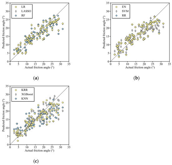
Figure 4.
Performance comparison of nine candidate base learners: (a) LR, LASSO, and RF; (b) EN, SVM, and RR; (c) KRR, XGBoost, and KNN.
The nine candidate base learners were further grouped into three subsets, with their corresponding results presented in Figure 4a–c. Such grouping facilitates clearer identification of the performance prioritization among these learners. As observed in Figure 4a, data points from the LR, LASSO, and RF learners cluster tightly along the 1:1 reference line, where predicted values exactly match actual measurements. This indicates that the predictive qualities are relatively good for these three learners. For the EN, SVM, and RR learners in Figure 4b, data points exhibit moderate dispersion around the reference line, reflecting that their performances are relatively intermediate. In contrast, Figure 4c shows that the KRR, XGBoost, and KNN learners produce results with the most pronounced deviation from the reference line, demonstrating the worst predictive qualities among the nine learners. All these results indicate that in a specific scenario, the performance of base learners varies significantly. That is why the prioritization of base learners is necessary to develop a Green AI model.
To further quantify the performances of the nine candidates, the R-squared (R2), root mean square error (RMSE), and mean absolute error (MAE) were used. The associated definitions are given as
where yi and ŷi are the ith measured value and predictive value, respectively; ȳ is the mean measured value; n is the number of training data or testing data. Note that the definition of MAE has been given in Equation (2), serving as the loss function. As indicated by the mathematical definitions, larger R2 values and lower RMSE/MAE values signify superior predictive quality.
Performance metrics on testing data for all nine candidates are summarized in Table 4. Consistent to the observations in Figure 4, based on R2, the prioritization generally follows: LR > LASSO > RF > EN > SVM > RR > KRR > XGBoost > KNN. The order is similar, based on RMSE and MAE. The maximum values of RMSE and MAE were produced by the KNN learner, while the minimum values were produced by the LR learner. Due to the consistency among R2, RMSE, and MAE, the performance of each model was simply evaluated using R2 in a later section of this study. Learner performance may just slightly vary between the testing data and train data. Therefore, in this study, it is plausible to make comparisons among different model architectures consistently using the testing data.
Table 4.
Performance quantification of nine candidate base learners.
To verify the effectiveness of the above prioritization, nine candidate base learners were categorized into the following three groups: (1) LR, LASSO, and RF learners (i.e., best learners), (2) EN, SVM, and RR learners (i.e., the medium learners); (3) KRR, XGBoost, and KNN learners (i.e., the worst learners). Three AI models were then constructed, each using one group as base learners. To isolate the impact of base learner quality, all models adopted the stacking strategy with a GBT meta learner. These models maintained identical configurations in terms of base learner quantity and ensemble strategy, with the only variation on the base learner composition. Figure 5 plots the predicted friction angle by these models against the actual measurement. Notably, all data points distributed tightly around the reference line, demonstrating that ensemble learning technique significantly enhances predictive quality, even when using the worst learners.
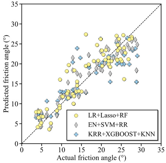
Figure 5.
Performance comparison among models integrating three different base learners.
To further quantify performance, metrics derived from Equations (2)–(4) were calculated for each model, with results summarized in Table 5. For comparison, the performance of the LR learner is also included as a baseline. As expected, the best learners produce the highest predictive quality, followed by the medium learners and the worst learners. With the aid of ensemble learning, they also surpass the standalone LR learner. Accordingly, R2 is dropped from 0.812 to 0.781. This hierarchy confirms that integrating high-performing learners was superior to integrating low-performing learners. More importantly, it provides compelling evidence that the above prioritization effectively guides the selection of base learners in constructing a Green AI model here.
Table 5.
Performance quantification of models integrating three different base learners.
While the above analysis has clearly validated the prioritization of base learners via deterministic performance metrics (i.e., R2, RMSE, and MAE), other performance metrics, including performance variance, confidence interval, and cross-validation dispersion, were not measured for the learners or models. The consideration of these additional metrics can better estimate the model uncertainty and robustness and can subsequently provide a more comprehensive comparison among different models. Therefore, in a future study, the performances of the learners or models will be re-evaluated.
4.2. Results by 2nd Stage Optimization on Base Learner Number
Second stage optimization aims to determine the optimal number of base learners, which is critical to our Green AI model here, as to minimize redundant computational cost. To this purpose, five candidate models were further constructed, integrating two to six base learners. The selection of base learners strictly followed the prioritization from the first stage; that is, for a model integrating N base learners, the top N candidates in Table 4 were selected. Predictive performances of these models are presented in Figure 6. For a comprehensive comparison, the performance of a standalone LR learner, which can be regarded as the model with only one base learner, is also included in Figure 6. Figure 6a presents the results with one to three base learners. Notably, the performance improved with an increase in the number of learners. In this time, the data points predicted by the LR learner are relatively far away from the diagonal, whereas the data points under three base learners cluster much closer to this line. Figure 6b further presents the results under four to six base learners. The three types of data points largely overlap with each other, signifying that their performances are nearly identical. Thus, within the range of four to six base learners, increasing the number of base learners no longer yields a significant improvement in predictive quality. This finding validates that there exists an optimal number of base learners, which balances the accuracy and computational efficiency.
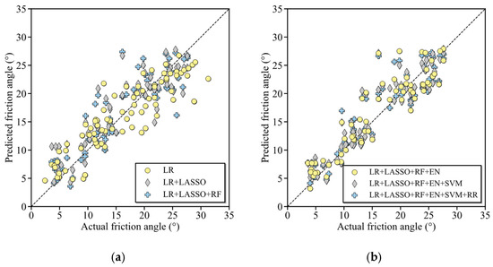
Figure 6.
Performance comparison among models integrating different numbers of base learners: (a) 1 to 3 learners; (b) 4 to 6 learners.
To further validate the observations from Figure 6, the performances of these six models (integrating one to six base learners) were quantitatively assessed again using Equations (2) to (4). Additionally, Figure 7 visualizes the trends of R2, RMSE, and MAE as functions of the number of base learners, providing a clear depiction of how model performance evolves with increasing complexity. As shown in Figure 7, the R2 value reaches a peak of 0.881 on the testing dataset when four base learners are integrated. Note that the value has exceeded those of existing AI models for shear strength parameters in the literature (see Table 2). Coincidently, this setting also corresponds to the lowest RMSE and MAE, indicating the best overall prediction accuracy; that is RMSE = 2.954° and MAE = 2.222°. For models with more than four base learners, the R2 curve exhibits a slight decline, while RMSE and MAE show only marginal increases. This pattern confirms the existence of an optimal number of base learners; that is, the performance improves monotonically below four learners, but additional learners above this threshold yield diminishing returns. Such a finding underscores the importance of balancing model complexity and generalization ability in Green AI model establishment.
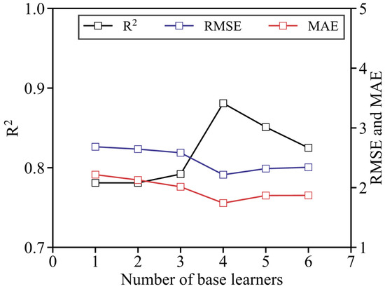
Figure 7.
Influence of base learner number on predictive quality on testing dataset.
To elucidate the existence of an optimal number of base learners, Figure 8 presents the evolution of learning curves (i.e., the evolution of MAE loss defined in Equation (1)) for models integrating two, four (optimal number), and six base learners, along with the iteration during training (as indicated by the loop in Figure 3). The two-learner model converges rapidly as iterations increase, yet its final MAE loss remains the highest among the three. In contrast, the four-learner model exhibits smoother convergence and achieves the lowest steady-state MAE loss. Meanwhile, the six-learner model shows more pronounced fluctuations throughout training, with a final loss that is higher than the four-learner model but lower than the two-learner one. This phenomenon arises because integrating more base learners introduces a higher-dimensional parameter space and more complex nonlinear interactions, which compromises training efficiency. Such training difficulties can be potentially mitigated by expanding dataset size or adopting advanced parameter update strategies, which will be systematically explored in future research.
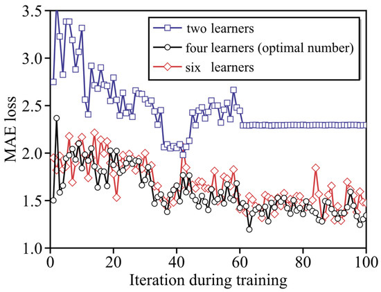
Figure 8.
Influence of base learner number on learning curve.
4.3. Results by 3rd Optimization of Ensemble Stragety and Energy-Saving Estimation
The third stage optimization targets to identify the optimal ensemble strategy. Besides stacking strategy with GBT meta learner, as mentioned, meta learners including LR, LASSO, and RF were also evaluated herein. It is attributed to their superior performance serving as the base learner, which has been validated in Section 4.1. Additionally, the voting strategy was examined and compared and it should be noted that the associated model maintained the same base learners as those with stacking strategy. The bagging strategy was also adopted for model construction. However, since the bagging strategy is designed for homogeneous base learners, four LR base learners were used instead in this case. Despite this adjustment, this setup still offers insights into how ensemble strategies influence performance.
Performance metrics of these models (i.e., R2, RMSE, and MAE) are summarized in Table 6. Again, the baseline by LR learner is included as well. Notably, the six models exhibit comparable results, with the difference on R2 value only limited in 0.1. Among them, stacking strategy using a GBT meta learner again produced the best performance, which aligns well with the finding in prior research [53]. When serving as the meta learner, the LR model again outperformed LASSO and RF models, which mirrors the prioritization in Section 4.1 and further validates the consistency of model performance across roles. The voting strategy achieved an R2 value of 0.831. Its moderate gap from the stacking-based results highlights that ensemble strategy has diminished importance after optimal base learner selection. The bagging strategy yielded the lowest performance. This is attributed to its reliance on homogeneous LR base learners, which lacked the synergistic benefits of heterogeneous model combinations. Collectively, the marginal impact of ensemble strategy observed here underscores the primacy of base learner optimization in determining the architecture of the Green AI model in this study.
Table 6.
Performance quantification of models with different ensemble strategies.
Based on the three-stage optimization via the greedy algorithm, the model architecture was finalized. In this optimized model, the LR, LASSO, RF, and EN base learners and the stacking strategy with a GBT meta learner were employed. This model embodies greenness and energy efficiency in two key aspects. First, the energy consumption to obtain output parameters, which accounts for highest consumption in the traditional ground investigation, can be significantly reduced. Second, it delivers superior generative quality under equivalent energy consumption. To further validate the second claim, a comprehensive examination on potential models with the 9 candidate base learners and 6 candidate ensemble strategies was conducted. A total of 2564 models with different architectures could theoretically be constructed. To balance computational efficiency while retaining representativeness, 300 AI models were constructed via Monte Carlo manner, without any optimization by greedy algorithm. In these models, the architecture was randomly produced from the pool of nine candidate base learners and six ensemble strategies. At least one of the three components, i.e., the number of base learners, the selection of base learners, and the ensemble strategy, is different between each two models. The performance metrics (i.e., R2, RMSE, and MAE) of all the 300 models on the testing dataset were estimated.
Histogram of R2 for the 300 models are further given in Figure 9. The number of models whose R2 falls at a certain value range was counted, and then the proportion term in Figure 9 was determined as this number divided by the total model number (i.e., 300). As depicted, the R2 values of some models are below 0.7, since the worst-performing learners were incorporated into the model. Very few models could exceed 0.85. The mean value of R2 for these potential models is 0.787 and the standard deviation is 0.075. Notably, the performance of our optimized model is located firmly in the top percentile of the distribution, verifying that the three-stage optimization approach is effective in identifying high-performing model architecture. The results revealed by Figure 9 are representative since the 300 models (out of 2564 models) have been examined. Nevertheless, sensitivity analysis of these results will be provided in the future.
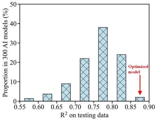
Figure 9.
Histogram of the predictive qualities among 300 AI models.
Finally, the energy consumption and saving by our Green AI model was estimated to examine its effectiveness in transforming traditional ground investigation. The estimated results are summarized in Table 7. It can be seen that following the traditional manner, the consumed energy to acquire strength parameters by direct shear test from 918 soil samples was 183,600 Wh. Using our Green AI model in the computer station of Dell PowerEdge R760, the energy consumption is significantly reduced to only 257 Wh, i.e., a reduction greater than 99%. This number has demonstrated the effectiveness and importance of introducing AI into the traditional practice of geotechnical engineering. The total energy cost for all tests (i.e., the cost to acquire the fifteen parameters in Table 2) was further estimated as 259,090 Wh. Using our model, the total energy cost (i.e., the summation of the costs from the model and other tests for input parameters) was reduced to 75,747 Wh; that is, the energy consumption is reduced by 71%, indicating that it is worth developing the Green AI model here. So far, this study focused on energy saving by comparing the AI model to traditional investigation practice with only laboratory tests. As mentioned, in-situ tests (e.g., SPT or CPT tests) are alternative to laboratory tests, which were, however, not provided in the ground investigation in the project of Huangpu Tram Line 2. Therefore, in the future study, a more comprehensive comparison will be made across the AI model, in-situ test, and laboratory tests.
Table 7.
Energy saving estimation for ground investigation.
The above analysis is still limited to energy saving via Green AI model. Indeed, a broader sustainability framework can be established by quantifying the carbon footprint reduction subsequently. According to Ministry of Ecology and Environment of China, the power carbon footprint factor is 0.6205 kg CO2/kWh on average [54]. Since 183.3 kWh can be saved using our model, the emission of almost 0.11t CO2 can be reduced during the laboratory testing stage of ground investigation. In addition, lifecycle implications can be provided, and more basic data at different stages of ground investigation should be collected to perform the evaluation in the future.
5. Conclusions
This study aims to explore the potential of Green AI for promoting energy-efficient ground investigation, and therefore a Green AI model for subsurface data prediction was established. The preliminary salient findings are as follows:
(1) The model embodies greenness in two aspects. First, the energy consumption to obtain output parameters (i.e., the shear strength parameters, which account for highest energy use in the traditional ground investigation) was reduced. Second, under equivalent energy consumption, the model demonstrates promising predictive quality with R2 = 0.881 on the testing dataset, which exceeds the performances of existing AI models for shear strength parameters in the literature (i.e., Table 2).
(2) The model architecture was designed based on ensemble learning, and thereby the model integrated the strengths of commonly used AI models. Following the Green AI concept, the architecture was further optimized by using the greedy algorithm, and the optimal selection of base learners and ensemble strategy was identified here.
(3) In this study, base learner selection benefited from prioritization, since integrating superior learners (e.g., LR, LASSO, and RF with R2 ≥ 0.758) may outperform integrating inferior learners (e.g., KRR, XGBoost, and KNN with R2 ≤ 0.692). There was an optimal number of base learners, since more learners may complicate the model network and reduce training efficiency. Upon the optimization of base learner, the influence of ensemble strategy became marginal.
(4) With this Green AI model, the energy consumption to acquire the shear strength parameters was reduced by 99% (using the ZJ-A direct shear test as a baseline). The consumption of entire ground investigation was reduced by 71%, demonstrating the effectiveness of introducing AI for energy-efficient geotechnical engineering.
Though this work provides preliminary insights into Green AI model for ground investigation, there are several limitations which constrain the broader generalization of the findings. One of the limitations is that the dataset was collected only from Huangpu Tram Line 2 in Guangzhou, South China. For other places in China, the soil parameter correlations and energy consumption patterns could differ significantly. In addition, the architecture optimization using greedy algorithms may reach the local optima, rather than the global optima. This possibility may be encountered in other scenarios. As mentioned, the estimation of energy saving exhibited some limitations as well, since the indirect field cost was not considered.
All these issues will be addressed in the future study. First, a national or even international soil database will be established by collecting data from other projects and using data from the literature. Thereby, the generalization of our Green AI model can be further enhanced by training on the expanded dataset. Second, an improved optimization method should be proposed to explore the best performing model architecture and to avoid reaching the local optima. Finally, more aspects (e.g., the reduction in borehole drilling) will be considered to estimate the energy saving for ground investigation, when adopting our Green AI model.
Besides addressing the above limitations in this study, a pathway of transferring our model to a new site investigation should be explored, especially when some new kinds of soils are encountered. Our model is transferable to a new site using following steps. For a site similar to the one here, a small number of soil testing data (e.g., via direct shear test) should be first collected from the new site. Then, our pre-trained model in this study can be fine-tuned using these new site data. Changes in performance metrics (e.g., R2, RMSE, and MAE) before and after fine-tuning will be evaluated. This will quantify the model adaptability to new scenarios and determine the minimum number of new site samples required for reliable transfer. For a new site where the soil types/parameters differ significantly from those here, some techniques such as domain-adversarial training (DAT) can be applied to align the feature distributions of the source domain (Guangzhou data) and target domain (new site data), subsequently transferring our model to a new site. The above pathway will be examined in the future study.
Author Contributions
Conceptualization, S.Z.; Data curation, X.Q.; Formal analysis, P.T.; Funding acquisition, Z.L. (Zhi Lan); Investigation, Y.S.; Methodology, Z.L. (Zhili Li); Project administration, X.Q.; Resources, Z.L. (Zhili Li) and Z.L. (Zhi Lan); Software, P.T.; Supervision, Z.L. (Zhi Lan); Validation, Y.S.; Visualization, P.T.; Writing—original draft, S.Z.; Writing—review and editing, P.T. and Z.L. (Zhi Lan). All authors have read and agreed to the published version of the manuscript.
Funding
This research was supported by Research Funding of Guangzhou Metro Design and Research Institute Co., Ltd. (KY-2021-045), Shenzhen Science and Technology Program (Grant Nos. GXWD20231129105817002, GXWD20220818152909001, and GXWD20231130125225001), Research Project of China State Railway Group Co., Ltd. (K2023G04).
Data Availability Statement
The original contributions presented in this study are included in the article. Further inquiries can be directed to the corresponding author.
Conflicts of Interest
Authors Siyuan Zhang, Zhili Li, Xiang Qiu, Yaohua Sui and Zhi Lan were employed by the company Guangzhou Metro Design & Research Institute Co., Ltd. The remaining author declare that the research was conducted in the absence of any commercial or financial relationships that could be construed as a potential conflict of interest.
References
- Das, B.M.; Sivakugan, N. Fundamentals of Geotechnical Engineering; Cengage Learning: Independence, KY, USA, 2017. [Google Scholar]
- Ng, C.W.; Liu, J.; Chen, R. Numerical investigation on gas emission from three landfill soil covers under dry weather conditions. Vadose Zone J. 2015, 14, vzj2014-12. [Google Scholar] [CrossRef]
- Liu, L.-L.; Xu, Y.-B.; Zhu, W.-Q.; Zhang, J. Effect of copula dependence structure on the failure modes of slopes in spatially variable soils. Comput. Geotech. 2024, 166, 105959. [Google Scholar] [CrossRef]
- Shi, X.; Liu, K.; Yin, J. Effect of initial density, particle shape, and confining stress on the critical state behavior of weathered gap-graded granular soils. J. Geotech. Geoenviron. Eng. 2021, 147, 04020160. [Google Scholar] [CrossRef]
- Härtl, J.; Ooi, J.Y. Experiments and simulations of direct shear tests: Porosity, contact friction and bulk friction. Granul. Matter 2008, 10, 263–271. [Google Scholar] [CrossRef]
- Tai, P.; Indraratna, B.; Rujikiatkamjorn, C.; Chen, R.; Li, Z. Cyclic behaviour of stone column reinforced subgrade under partially drained condition. Transp. Geotech. 2024, 47, 101281. [Google Scholar] [CrossRef]
- Chen, R.; Luo, Z.; Zhang, L.; Li, Z.; Tan, R. A new flexible-wall triaxial permeameter for localized characterizations of soil suffusion. Q. J. Eng. Geol. Hydrogeol. 2025, 58, qjegh2023-124. [Google Scholar] [CrossRef]
- Ladd, R. Preparing test specimens using undercompaction. Geotech. Test. J. 1978, 1, 16–23. [Google Scholar] [CrossRef]
- Ng, C.W.; Liu, J.; Chen, R.; Xu, J. Physical and numerical modeling of an inclined three-layer (silt/gravelly sand/clay) capillary barrier cover system under extreme rainfall. Waste Manag. 2015, 38, 210–221. [Google Scholar] [CrossRef]
- Zeng, Y.; Shi, X.; Zhao, J.; Bian, X.; Liu, J. Estimation of compression behavior of granular soils considering initial density effect based on equivalent concept. Acta Geotech. 2025, 20, 1035–1048. [Google Scholar] [CrossRef]
- Chen, R.; Ng, C.W.W. Impact of wetting–drying cycles on hydro-mechanical behavior of an unsaturated compacted clay. Appl. Clay Sci. 2013, 86, 38–46. [Google Scholar] [CrossRef]
- Zhang, J.; Liu, W.; Yu, Q.; Zhu, Q.-Z.; Shao, J.-F. A micromechanical model for induced anisotropic damage-friction in rock materials under cyclic loading. Int. J. Rock Mech. Min. Sci. 2025, 186, 106014. [Google Scholar] [CrossRef]
- Li, Z.; Zhang, Y.; Chen, R.; Tai, P.; Zhang, Z. Numerical investigation of morphological effects on crushing characteristics of single calcareous sand particle by finite-discrete element method. Powder Technol. 2025, 453, 120592. [Google Scholar] [CrossRef]
- Shi, X.; Zhao, J. Practical estimation of compression behavior of clayey/silty sands using equivalent void-ratio concept. J. Geotech. Geoenviron. Eng. 2020, 146, 04020046. [Google Scholar] [CrossRef]
- Zhang, J.; Liu, W.; Zhu, Q.; Shao, J.-F. A novel elastic–plastic damage model for rock materials considering micro-structural degradation due to cyclic fatigue. Int. J. Plast. 2023, 160, 103496. [Google Scholar] [CrossRef]
- Niu, Q.; Revil, A.; Li, Z.; Wang, Y.-H. Relationship between electrical conductivity anisotropy and fabric anisotropy in granular materials during drained triaxial compressive tests: A numerical approach. Geophys. J. Int. 2017, 210, 1–17. [Google Scholar] [CrossRef]
- Sivrikaya, O.; Toğrol, E. Determination of undrained strength of fine-grained soils by means of SPT and its application in Turkey. Eng. Geol. 2006, 86, 52–69. [Google Scholar] [CrossRef]
- Jamiolkowski, M.; Lo Presti, D.; Manassero, M. Evaluation of relative density and shear strength of sands from CPT and DMT. In Soil Behavior and Soft Ground Construction; American Society of Civil Engineers: Reston, VA, USA, 2003; pp. 201–238. [Google Scholar]
- Shi, X.; Xu, J.; Guo, N.; Bian, X.; Zeng, Y. A novel approach for describing gradation curves of rockfill materials based on the mixture concept. Comput. Geotech. 2025, 177, 106911. [Google Scholar] [CrossRef]
- Wang, H.; Chen, R.; Leung, A.K.; Garg, A.; Jiang, Z. Pore-based modeling of hydraulic conductivity function of unsaturated rooted soils. Int. J. Numer. Anal. Methods Geomech. 2025, 49, 1790–1803. [Google Scholar] [CrossRef]
- Pentoś, K.; Mbah, J.T.; Pieczarka, K.; Niedbała, G.; Wojciechowski, T. Evaluation of multiple linear regression and machine learning approaches to predict soil compaction and shear stress based on electrical parameters. Appl. Sci. 2022, 12, 8791. [Google Scholar] [CrossRef]
- Puri, N.; Prasad, H.D.; Jain, A. Prediction of geotechnical parameters using machine learning techniques. Procedia Comput. Sci. 2018, 125, 509–517. [Google Scholar] [CrossRef]
- Tziachris, P.; Aschonitis, V.; Chatzistathis, T.; Papadopoulou, M.; Doukas, I.D. Comparing machine learning models and hybrid geostatistical methods using environmental and soil covariates for soil pH prediction. ISPRS Int. J. Geo-Inf. 2020, 9, 276. [Google Scholar] [CrossRef]
- Li, J.; Sun, J.; Zhang, Z.; Li, Z. Comparative investigation of torsional interactive behaviours between suction anchors and clayey ground by centrifugal tests. Ocean Eng. 2025, 341, 122676. [Google Scholar] [CrossRef]
- Li, K.-Q.; Liu, Y.; Kang, Q. Estimating the thermal conductivity of soils using six machine learning algorithms. Int. Commun. Heat Mass Transf. 2022, 136, 106139. [Google Scholar] [CrossRef]
- Feng, Y.; Cui, N.; Hao, W.; Gao, L.; Gong, D. Estimation of soil temperature from meteorological data using different machine learning models. Geoderma 2019, 338, 67–77. [Google Scholar] [CrossRef]
- Araya, S.N.; Ghezzehei, T.A. Using machine learning for prediction of saturated hydraulic conductivity and its sensitivity to soil structural perturbations. Water Resour. Res. 2019, 55, 5715–5737. [Google Scholar] [CrossRef]
- Samui, P.; Sitharam, T. Machine learning modelling for predicting soil liquefaction susceptibility. Nat. Hazards Earth Syst. Sci. 2011, 11, 1–9. [Google Scholar] [CrossRef]
- Achieng, K.O. Modelling of soil moisture retention curve using machine learning techniques: Artificial and deep neural networks vs support vector regression models. Comput. Geosci. 2019, 133, 104320. [Google Scholar] [CrossRef]
- Zhang, P.; Yin, Z.-Y.; Jin, Y.-F. Machine learning-based modelling of soil properties for geotechnical design: Review, tool development and comparison. Arch. Comput. Methods Eng. 2022, 29, 1229–1245. [Google Scholar] [CrossRef]
- Li, Z.; Qi, Z.; Ling, J.; Liu, Y.; Guo, H.; Xu, T. A pragmatic modelling framework for long-term deformation analyses of urban tunnel under multi-source cyclic loads. Tunn. Undergr. Space Technol. 2026, 167, 107029. [Google Scholar] [CrossRef]
- Das, S.K.; Basudhar, P.K. Prediction of residual friction angle of clays using artificial neural network. Eng. Geol. 2008, 100, 142–145. [Google Scholar] [CrossRef]
- Pham, B.T.; Nguyen-Thoi, T.; Ly, H.-B.; Nguyen, M.D.; Al-Ansari, N.; Tran, V.-Q.; Le, T.-T. Extreme learning machine based prediction of soil shear strength: A sensitivity analysis using Monte Carlo simulations and feature backward elimination. Sustainability 2020, 12, 2339. [Google Scholar] [CrossRef]
- Pham, B.T.; Hoang, T.-A.; Nguyen, D.-M.; Bui, D.T. Prediction of shear strength of soft soil using machine learning methods. Catena 2018, 166, 181–191. [Google Scholar] [CrossRef]
- Zhu, L.; Liao, Q.; Wang, Z.; Chen, J.; Chen, Z.; Bian, Q.; Zhang, Q. Prediction of soil shear Strength parameters using combined data and different machine learning models. Appl. Sci. 2022, 12, 5100. [Google Scholar] [CrossRef]
- Verdecchia, R.; Sallou, J.; Cruz, L. A systematic review of Green AI. Wiley Interdiscip. Rev. Data Min. Knowl. Discov. 2023, 13, e1507. [Google Scholar] [CrossRef]
- Li, Y.; Rahardjo, H.; Satyanaga, A.; Rangarajan, S.; Lee, D.T.-T. Soil database development with the application of machine learning methods in soil properties prediction. Eng. Geol. 2022, 306, 106769. [Google Scholar] [CrossRef]
- Chow, J.K.; Li, Z.; Su, Z.; Wang, Y.-H. Characterization of particle orientation of kaolinite samples using the deep learning-based technique. Acta Geotech. 2022, 17, 1097–1110. [Google Scholar] [CrossRef]
- Hengl, T.; Mendes de Jesus, J.; Heuvelink, G.B.; Ruiperez Gonzalez, M.; Kilibarda, M.; Blagotić, A.; Shangguan, W.; Wright, M.N.; Geng, X.; Bauer-Marschallinger, B. SoilGrids250m: Global gridded soil information based on machine learning. PLoS ONE 2017, 12, e0169748. [Google Scholar] [CrossRef]
- Zhang, X.; Li, Z.; Sui, Y.; Liu, C.; Li, Z. Hybrid soil strength prediction model for geotechnical ground investigation using convolutional neural network and ensemble learning. J. Phys.: Conf. Ser. 2024, 2816, 012066. [Google Scholar] [CrossRef]
- Cao, M.-T.; Hoang, N.-D.; Nhu, V.H.; Bui, D.T. An advanced meta-learner based on artificial electric field algorithm optimized stacking ensemble techniques for enhancing prediction accuracy of soil shear strength. Eng. Comput. 2022, 38, 2185–2207. [Google Scholar] [CrossRef]
- Liu, L.-L.; Yin, H.-D.; Xiao, T.; Huang, L.; Cheng, Y.-M. Dynamic prediction of landslide life expectancy using ensemble system incorporating classical prediction models and machine learning. Geosci. Front. 2024, 15, 101758. [Google Scholar] [CrossRef]
- Lin, S.; Zheng, H.; Han, B.; Li, Y.; Han, C.; Li, W. Comparative performance of eight ensemble learning approaches for the development of models of slope stability prediction. Acta Geotech. 2022, 17, 1477–1502. [Google Scholar] [CrossRef]
- Bian, X.; Fan, Z.; Liu, J.; Li, X.; Zhao, P. Regional 3D geological modeling along metro lines based on stacking ensemble model. Undergr. Space 2024, 18, 65–82. [Google Scholar] [CrossRef]
- Rabbani, A.; Samui, P.; Kumari, S. Implementing ensemble learning models for the prediction of shear strength of soil. Asian J. Civ. Eng. 2023, 24, 2103–2119. [Google Scholar] [CrossRef]
- Schwartz, R.; Dodge, J.; Smith, N.A.; Etzioni, O. Green AI. Commun. ACM 2020, 63, 54–63. [Google Scholar] [CrossRef]
- Zhang, X.; Li, Z.; Zhang, S.; Sui, Y.; Liu, C.; Xue, Z.; Li, Z. Comparative Investigation of Axial Bearing Performance and Mechanism of Continuous Flight Auger Pile in Weathered Granitic Soils. Buildings 2023, 13, 2707. [Google Scholar] [CrossRef]
- Bian, X.; Gao, Z.; Zhao, P.; Li, X. Quantitative analysis of low carbon effect of urban underground space in Xinjiekou district of Nanjing city, China. Tunn. Undergr. Space Technol. 2024, 143, 105502. [Google Scholar] [CrossRef]
- Shi, X.; Nie, J.; Zhao, J.; Gao, Y. A homogenization equation for the small strain stiffness of gap-graded granular materials. Comput. Geotech. 2020, 121, 103440. [Google Scholar] [CrossRef]
- Henderi, H.; Wahyuningsih, T.; Rahwanto, E. Comparison of Min-Max normalization and Z-Score Normalization in the K-nearest neighbor (kNN) Algorithm to Test the Accuracy of Types of Breast Cancer. Int. J. Inform. Inf. Syst. 2021, 4, 13–20. [Google Scholar] [CrossRef]
- Bian, X.; Ren, Z.; Zeng, L.; Zhao, F.; Yao, Y.; Li, X. Effects of biochar on the compressibility of soil with high water content. J. Clean. Prod. 2024, 434, 140032. [Google Scholar] [CrossRef]
- Lin, S.; Liang, Z.; Zhao, S.; Dong, M.; Guo, H.; Zheng, H. A comprehensive evaluation of ensemble machine learning in geotechnical stability analysis and explainability. Int. J. Mech. Mater. Des. 2024, 20, 331–352. [Google Scholar] [CrossRef]
- Susan, S.; Kumar, A.; Jain, A. Evaluating heterogeneous ensembles with boosting meta-learner. In Proceedings of the Inventive Communication and Computational Technologies: Proceedings of ICICCT 2020, Namakkal, India, 28–29 May 2020; pp. 699–710. [Google Scholar]
- Ministry of Ecology and Environment of the People’s Republic of China. Announcement on the Release of 2023 Power Carbon Footprint Factor Data. 2025. Available online: https://www.mee.gov.cn/xxgk2018/xxgk/xxgk01/202501/t20250123_1101226.html (accessed on 11 August 2025).


Disclaimer/Publisher’s Note: The statements, opinions and data contained in all publications are solely those of the individual author(s) and contributor(s) and not of MDPI and/or the editor(s). MDPI and/or the editor(s) disclaim responsibility for any injury to people or property resulting from any ideas, methods, instructions or products referred to in the content. |
© 2025 by the authors. Licensee MDPI, Basel, Switzerland. This article is an open access article distributed under the terms and conditions of the Creative Commons Attribution (CC BY) license (https://creativecommons.org/licenses/by/4.0/).