Article

Calibration of a Multiphase Poroelasticity Model Using Genetic Algorithms

by
Monika Bartlewska-Urban
* and
Irena Bagińska
*
Faculty of Geoengineering, Mining and Geology, Wroclaw University of Science and Technology, 50-370 Wroclaw, Poland
*
Authors to whom correspondence should be addressed.
Appl. Sci. 2025, 15(22), 11972; https://doi.org/10.3390/app152211972
Submission received: 5 October 2025 / Revised: 20 October 2025 / Accepted: 4 November 2025 / Published: 11 November 2025
(This article belongs to the Special Issue Machine Learning and Soft Computing: Current Trends and Applications)

Abstract

Clibration of constitutive models is a critical step in geotechnical design, ensuring that numerical predictions accurately reproduce observed behavior. This study explores the use of Genetic Algorithms (GAs) for the calibration of Biot’s poroelastic model based on oedometer test data. A two-stage calibration procedure was applied. In Stage 1, when five parameters were varied simultaneously, the results showed strong parameter intercorrelation and structural non-identifiability, as different parameter sets produced nearly identical objective function values. To address this limitation, an identifiability analysis was performed, leading to parameter reduction. In Stage 2, only A, R, and k were calibrated, with N and H fixed, which resulted in stable and interpretable solutions. The GA-based approach demonstrated convergence, the absence of local minima, and good agreement with experimental data. The study highlights both the potential and the current limitations of GA-based calibration and should be regarded as a proof-of-concept rather than a complete identifiability study.

1. Introduction

A critical stage in the use of mathematical models in geoengineering is the determination of the values of the effective model parameters in order for the obtained results to most accurately reflect the real processes. The starting point for our experimental research was the Biot multiphase medium model, assuming that the porous solid body includes hydraulically interconnected pores or microcracks enabling the flow of a liquid or a gas [1]. This paper presents a methodology for determining the effective parameters of the Biot-Darcy model. The rheological properties of soils and rocks have been the subject of many research projects and publications. The phenomena involved there are described using rheological models of continuous medium mechanics. The starting point is a multiphase medium model, assuming that the solid body includes hydraulically interconnected pores or microcracks enabling the filtration flow of a liquid or a gas. The mathematical model of creep in porous media, defined as a multicomponent diphase body, was first introduced by Biot [2,3] and later analyzed using asymptotic homogenization for poorly compressible pore fluids. For this purpose, Łydżba [4], Auriault [5], Bensoussan et al. [6], Auriault and Sanchez Palencia [7] used the methods for periodic structures, while Kröner [8], Rubin-stein and Torquato [9] used statistical methods. For the case where the medium pores are filled with a gas, a mathematical model based on the asymptotic homogenization method was presented by Auriault et al. [10]. One of the fundamental assumptions of porous medium mechanics is the porous medium continuity postulate, which is a considerable simplification when this theory is applied to soils. Despite this assumption, models describing the creep of the Biot body well represent the actual processes of deformation of cohesive soils (argillaceous and clayey soils and mudclays).

Related Works and Theoretical Background

Thermo-poroelastic processes in multiphase media, including temperature-driven consolidation, have been described by Uciechowska-Grakowicz [11], Uciechowska-Grakowicz and Strzelecki [12], and Strzelecki and Uciechowska [13], while anisotropy was analyzed by Zhang et al. [14] and porosity evolution by Chen et al. [15]. Bartlewska and Strzelecki [16,17] derived consolidation equations for the Biot model with a Kelvin–Voigt rheological skeleton, showing that, in addition to volumetric compressibility and shear elasticity, the viscosity of the soil skeleton plays a significant role.
Soil mechanics, as a major branch of geotechnical engineering, deals with one of the most challenging materials to describe mathematically—soil [18,19]. Due to its three-phase nature, soil requires advanced mathematical techniques to capture the physicochemical processes occurring in each of the three phases [20]. Among the computational techniques widely used in geotechnics, optimization methods have gained importance, especially for the calibration of constitutive models [21,22]. Considering the three fundamental components of such models—the plasticity criterion, the plastic potential, and the hardening law—calibration in this study was carried out on the basis of laboratory test results, which provided the experimental data for the inverse analysis. An effective approach to address these challenges is reverse analysis combined with an optimizing algorithm, which allows for the automatic calibration of model parameters. In particular, the highly coupled nature of the Biot model—with multiple interdependent parameters governing solid–fluid interactions—makes traditional gradient-based calibration methods unstable or inefficient. Genetic Algorithms provide a robust, derivative-free optimization framework capable of handling such nonlinearity and interparameter correlations.
Building on this theoretical and methodological background, the aim of this study is to present the application of genetic algorithms for calibrating the Biot poroelastic model. The results demonstrate that genetic algorithms are effective in the automatic determination of Biot’s parameters, even for complex rheological models.
Recent developments in computational intelligence have further expanded the capabilities of genetic algorithms (GAs) in inverse modeling and parameter estimation. Notably, enhancements in selection and crossover strategies have led to increased optimization robustness, even in high-dimensional spaces [23]. Hybrid methods combining GAs with surrogate machine learning models are also gaining attention due to their potential to reduce computational costs while maintaining accuracy [24]. In the context of constitutive model calibration, GA-based methods have proven successful for complex material behaviors [25]. Meanwhile, modern numerical methods for solving poroelasticity problems, such as the hybrid discontinuous Galerkin (HDG) approach, offer benchmarks for assessing the accuracy of simulation-based calibration workflows [26].
While previous studies have demonstrated the usefulness of GAs in geotechnical problems such as slope stability or triaxial compression test interpretation, their application to poroelastic models remains limited. In particular, the calibration of the Biot model—which requires handling multiphase interactions and parameter interdependencies—has not been addressed comprehensively. The novelty of this study therefore lies in extending GA-based calibration to the Biot poroelastic model, providing a framework that improves parameter identifiability, convergence, and robustness. These advancements support the relevance of the methodology proposed in this paper and highlight its potential for broader applications in geotechnical and multiphase material modeling.
Before transitioning to the mathematical formulation, it is important to clarify the physical meaning of the Biot model parameters used in this study. Table 1 summarizes their engineering interpretation, corresponding units, and typical magnitude ranges reported in the literature. This reference framework facilitates a better understanding of the calibration results presented in the following sections and underscores the physical plausibility of the identified parameters.
The parameter values listed in Table 1 are representative of cohesive and fine-grained soils, which are the focus of the present study. These parameters are subsequently calibrated and validated using oedometer test data as described in Section 5.

2. Mathematical Model of Porous Medium

The classical constitutive equations for a poroelastic material under isothermal conditions were formulated by Biot [2] and further developed by Biot and Willis [28], incorporating insights from Coussy’s research [29]. In this study, Biot′s effective parameters (known as Biot’s constants) are introduced for the first time with labels N, A, R, Q, and N. The initial formulation of the constitutive relations for a medium comprising a porous elastic framework and a liquid was as follows:
σ i j = 2 N ε i j + A ε δ i j + Q θ δ i j σ σ a = Q ε + R θ
where N and A are the Lamé constants for the porous medium’s skeleton, R is the modulus of volume elasticity of the liquid, Q is the coupling coefficient representing the interaction between the solid and liquid phases, σij is the stress tensor in the skeleton, associated with the total Representative Volume Element (RVE) surface and defined as effective stress tensor, σ is the stress in the liquid, also related to the total surface area of the RVE cross-section and similarly defined as effective stress, εij is the deformation tensor of the skeleton, ε = εij represents skeleton dilatation, and θ denotes liquid dilatation. Additionally, with pressure in the liquid denoted as p and porosity as fo, the pore pressure contribution in the liquid is given by the formula: σ = − fo p.
The consolidation equations were derived by Biot [2] and have the following form:
N 2 u i + M + N ε , i = H R σ , i k f 2 2 σ = 1 R σ ˙ H R ε ˙
where k f 2 = K , k—Darcy’s filtration coefficient, f—the skeleton’s porosity.
Srokosz [31] proposed using genetic computation techniques to tackle various geotechnical engineering challenges, such as scarp (a steep ground surface break) and slope stability and the interpretation of triaxial compression test results. He demonstrated that advanced numerical methods could effectively restore some traditional geotechnical solutions that have been around for decades but were not practically applied due to high computational costs. In this study, genetic algorithms were applied for the calibration of the Biot model using inverse analysis. The findings discussed in Section 6 could serve as a foundation for further exploration into applying genetic algorithms for analyzing the effective parameters of the Biot model, especially when considering the viscosity of the soil skeleton.

3. Genetic Algorithms

The dynamic progress of artificial intelligence makes it possible to use tools such as learning machines in engineering practice: geoengineering [32,33], medicine [34,35], broadly understood computer science and other fields [36,37]. The area of artificial intelligence devoted to algorithms that emerge automatically through self-learning builds a mathematical model based on sample data, called a training set, in order to make predictions or decisions. Genetic algorithms (GAs) can be defined as a group of numerical techniques inspired by natural information processing [38,39,40,41,42,43], which are classified among robust optimization methods that maintain effectiveness across diverse problems regardless of details. The effectiveness of genetic algorithms in solving complex optimization problems has been widely demonstrated in the literature [32], which makes them a suitable tool for automatic determination of effective parameters in poroelastic models. This adaptability stems from the fact that optimization is performed solely on the basis of the objective function value (Fc). The algorithm has no other information about the model or the process being modeled. This is a particularly interesting feature since owing to it, once a methodology is developed, it can be applied, practically without any modifications, to different rheological models and different experimental data. Another interesting feature of such algorithms is their ability to bypass local minima of objective functions, whereby the chance of finding a global optimum increases.
The terminology associated with genetic algorithms includes not only standard optimization terms but also terms borrowed from genetics. This is due to the way genetic algorithms function, which, as previously noted, mimics natural evolutionary processes [40,41,42,44]. Genetic algorithms work with variables that are represented by code sequences known as chromosomes. These sequences are made up of a collection of traits, or genes. Each gene is part of a (typically binary) alphabet chosen for the specific application, and the possible values for these traits are called alleles. The complete set of genetic information for a given element is referred to as its genotype. There are solutions that use structures consisting of two or three chromosomes. If an algorithm operates on data in the form of a single data sequence, the terms: chromosome and genotype are synonymous.
The data structures (code combinations) that genetic algorithms work with are translated into specific values for the variables, which are typically real or integer [41,42,44].
These variables are then evaluated using an objective function. The combination of parameters and their evaluation forms what is known as a phenotype. A collection of phenotypes at a particular stage of the optimization process is referred to as a population. Genetic operators are applied to generate the next populations, and these operators ensure that each new generation has a different set of genes compared to the previous one. Figure 1 provides a block diagram that illustrates the functioning of genetic algorithms, highlighting seven key steps in the process [45].
The first step in GA operation is the selection of an initial population, consisting of the initialization of an assigned number of chromosomes that form a set of starting points. The initialization most often takes place through the random selection of the values of consecutive genes [40,41,46].
The adaptation of chromosomes within a population is assessed based on the adaptation function values for all individuals in the current generation. This evaluation process occurs in several steps. Initially, chromosomes are translated into variable values using a suitable decoding method. These variables are then utilized to compute the objective function for every individual in the population. If the objective function assumes negative values and a maximum is sought, the function can be considered to be an adaptation function. In some cases (especially for the roulette wheel selection method), it is recommended to use scaling to obtain proper selectivity.
The stopping criteria are determined according to the optimization goals. In the most basic scenario, this involves performing a predetermined number of iterations or evaluating a specified number of points in the search space, or time out can be the condition. The algorithm can be stopped when there is no significant improvement in the results.
Chromosome selection is carried out to identify chromosomes for a parent pool, from which a new population (a set of solutions) is generated using genetic operators. Regardless of the specific method employed, the selection process is always based solely on the adaptation function values of the individuals. Three principal selection methods are distinguished: the roulette method, the tournament method, and the ranking method. The roulette method assigns probabilities proportional to fitness values [40,41]. The tournament method selects the best individual from a randomly chosen subset [41,42]. The ranking method assigns probabilities according to the ranking of individuals instead of raw fitness values [46,47].
The chromosomes from the individuals chosen for the parent pool undergo genetic operations, which results in the creation of a population of offspring. It is through the operations of the genetic operators that new points in the space of variables are generated and new solutions are created. Typically, two genetic operators are used: the crossover operator, which combines genetic material from two parents to generate offspring [40,41], and the mutation operator, which introduces random changes into the genes of an individual to preserve diversity and avoid premature convergence [42,48]. Among these, crossover plays the most important role in the optimization process.
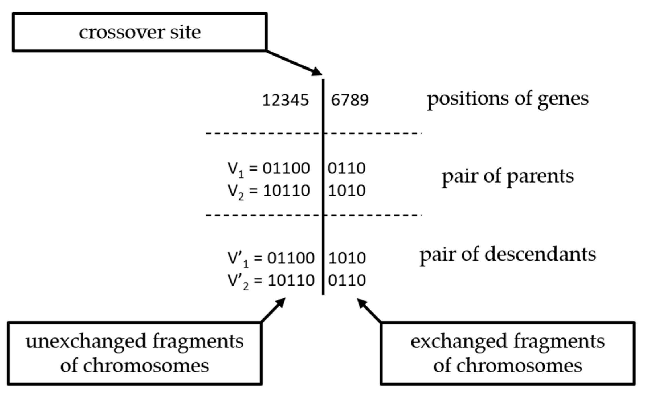
The crossover operator operates simultaneously on two chromosomes selected from a parental pool, causing the exchange of fragments of their chromosomes. One-two or multipoint crossing is possible. A flow diagram of the one-point crossover operator is shown in Figure 2.
Figure 2. Flow diagram of the one-point crossover operator used in the genetic algorithm. Mutation is performed on a gene with an assigned probability that causes a change in its state [41,42]. Mutation plays only a supporting role in crossing and should not occur more often than the latter [40,48]. The mutation operator can be applied to a parental pool before a new generation is created or to newly created individuals. Figure 3 shows schematically the mutation of a gene.
Applsci 15 11972 g002
Following the application of genetic operators, a new population is generated from the individuals. This new population then becomes the current one, and the objective function and adaptation function values are computed for it. The stopping criteria are subsequently evaluated, and if further computation is required, another iteration begins.
When the stopping criteria are met, the final result is produced. This result consists of the values of the decision variables corresponding to the chromosome with the highest (or lowest, if a minimum is desired) objective function value.
A binary encoding scheme was adopted to maintain compatibility with the discrete parameter ranges derived from laboratory data and to preserve computational simplicity in this proof-of-concept study. Although real-coded GA formulations are commonly used for continuous optimization problems, preliminary tests indicated that the binary scheme provided sufficient accuracy and numerical stability for the considered parameter sets. The described procedure formed the basis for the GA-based calibration framework presented in the following section.

4. The Methodology Adopted

The results from the oedometer tests were utilized as calibration data for the study. The calibration process was performed using a program developed by the authors that implements the classical genetic algorithm, along with the FlexPDE 6 software [49] for conducting finite element method (FEM) simulations required for the back analysis.
With this combination of software, calibration can be precisely conducted on the model, which is subsequently applied to real engineering problems. Furthermore, the capabilities of FlexPDE 6 software allow for the implementation of a sophisticated experimental design that involves the incremental loading of an oedometer sample.
To perform this calibration, the numerical implementation was carried out in the FlexPDE environment. A mathematical model was implemented using the FlexPDE program, which has been extensively tested in research conducted by the authors and has also been successfully applied in recent geomechanical and coupled process studies [50]. One can introduce any mathematical model into it by defining state variables, model equations, modeled area geometry, and boundary and initial conditions. For this kind of investigation, a very important feature of the FlexPDE program is the possibility of starting computations from an external control program and saving the results in a user-friendly format in a text file.
The optimization algorithm was developed as a standalone program written in C# using the .NET framework 4.8, designed to enable the calibration of any mathematical model using results from an external simulation software. In order to link the optimization procedure with the FEM simulations, the GA was implemented as a standalone C# program.
In the case of operation in tandem with the FlexPDE program, the objective function value is determined in a single simulation through the following steps:
  • the algorithm reads laboratory measurement results from a file;
  • from the basic file for the FlexPDE program the algorithm creates a model .pde file with entered values of the calibrated parameters;
  • the algorithm makes the Flex PDE program execute a simulation, the results of which are saved to a text file;
  • The algorithm waits for the simulation to end and then reads the simulation results; using the simulation and measurement results, the algorithm calculates the objective function value (a standard square estimator).
Additionally, a simplified permeability–porosity relation was introduced in the form k/Φ2 = K. This heuristic assumption was applied in order to reduce the number of free parameters in the calibration process, reflecting the proof-of-concept character of the present study. It is not intended to replace classical permeability–porosity models. For completeness, we now explicitly refer to well-established formulations such as the Kozeny–Carman equation [51,52,53], which will be considered in future extensions of the methodology.

5. Results of the Determination of Effective Parameters of the Biot Model

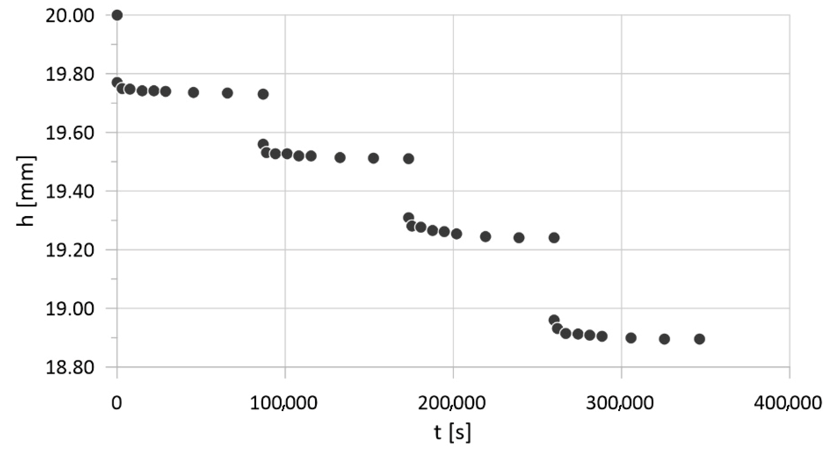
A diagram of the changes in the height of the sample is shown in Figure 4. The successive changes in sample height correspond to the successive changes in load. The time between successive load increments was approximately 24 h (86,400 s), which was sufficient for the sample height to stabilize before the next increment.

5.1. Simulation Parameters

Because of the number of necessary simulations to be carried out at this stage in the development of the method and the one-dimensional nature of the modeled phenomenon, the simulation was conducted in 1D space. A uniform one-dimensional finite element mesh consisting of 20 equally spaced nodes (element size = 1 mm) was used to discretize the specimen height. The analyzed material corresponds to a cohesive, low-permeability clayey soil tested in a standard oedometer experiment (ASTM D2435 [54]) with a sample height of 20 mm. As the model was one-dimensional, this mesh resolution was sufficient to ensure numerical stability and accuracy, and further refinement did not change the results. Each calibration required approximately 1000 simulations, with a single run taking between 10 and 30 s depending on parameter values. In the first stage, five Biot model parameters (N, A, R, H, k) all expressed in [Pa] and k [m/s] were varied, while in the second stage the number of calibrated variables was reduced to three (A, R, k), with N and H kept constant.
The following boundary conditions were adopted:
  • for the sample base—(x = 0): u = 0, θ = 0;
  • for the upper surface of the sample—(x = h = 20 mm): u′ = 0, θ = T(t).
Each calibration of a model should be preceded by an analysis of model identifiability in order to determine a set of parameters lending themselves to calibration. The methodology and results of such an analysis were presented in [27]. The investigations presented in the present paper focus on developing a universal calibration methodology (applicable to any experimental data) and verifying its effectiveness for highly complicated conditions in order to demonstrate its resistance also to errors in determining identifiability, since this is a problem which requires extensive theoretical knowledge and excellent knowledge of the model being calibrated.
Therefore, calibration was carried out in two stages. In the first stage, all the model parameters, i.e., N, A, R, H and k, were included. In the second stage, the number of calibrated parameters was reduced on the basis of an identifiability analysis, which consisted in assessing the sensitivity of the objective function to each parameter and identifying correlations between them. Parameters showing strong correlation and low sensitivity were excluded from calibration, as they could not be reliably identified [55,56]. As a result, only three parameters were calibrated: A, R and k. The other parameters were assumed constant (N = 1 × 10⁷ Pa and H = 3 × 10⁷ Pa), and the values of the remaining parameters were fitted during calibration to obtain a minimum of the objective function. The search ranges adopted for the particular parameters are shown in Table 2. The last column of this table shows the estimation accuracy, expressed as codon length, for each parameter. It should be noted that this identifiability analysis was performed in a qualitative, descriptive manner and not as a full statistical evaluation (e.g., Fisher Information Matrix or sensitivity matrices), consistent with the proof-of-concept scope of this study.

5.2. Algorithm Parameters

The classical genetic algorithm model with one-point crossover and two operators was adopted: a crossover operator (with a probability of 0.8 for a pair of chromosomes) and a mutation operator (with a probability of 0.02 for a single gene), following the classical formulations of GAs described by Holland [40], Goldberg [41], and Mitchell [42].
The roulette method, with the scaling and rejection of 10% of the worst chromosomes, was used as the selection method. The population size of 50 was adopted. The stopping criterion of the calibration process was defined as the lack of improvement in the objective function value for 5 consecutive generations (approximately 250 simulations). Additionally, a maximum number of generations was imposed to ensure termination in cases of slow convergence. This dual criterion provided both accuracy of calibration and computational efficiency.
The lengths of the codons for the particular parameters shown in Table 2 fix the chromosome length at 38 bits and at 24 bits for the particular stages. The total number of points which can be coded using this length amounts to 238 = 2.75 × 10¹¹ for the first stage and 224 = 1.68 × 10⁷ for the second stage.
Altogether 20 independent calibrations of the model were carried out. On average, it was necessary to recalculate 30–40 generations, i.e., to run about 1000 simulations. The program used for the computations made it possible to simultaneously perform computations on the individual processors (8 threads), whereby the total calibration process did not take longer than 1 h. The parameter values obtained in the first stage are shown in Table 3.
The values of the objective functions are on a similar level, whereas the values of the parameters differ greatly, as indicated by the computed standard deviations (SD). This shows that even when the calibration achieves comparable objective function values, the associated parameter sets may vary significantly, which reflects their intercorrelation and points to identifiability issues. It is interesting to note that in each of the cases, similar objective function values were obtained, confirming the effectiveness and convergence of the algorithm [57]. No local minimum was observed in the calibration of all the parameters. The calibration was based on 68 measuring points, and the obtained objective function values are expressed in terms of average simulation error for a single measuring point, shown in the last column of Table 3. The errors are at the level of measuring errors. The simulation results for the first series (Figure 5) show very good agreement with the experimental results. Moreover, they confirm the identical course of the simulations despite the considerably different parameter values.
To benchmark the calibrated results, we verified that the settlement–time curves reproduce the expected primary consolidation behavior for cohesive soils and that the numerical simulations closely follow the experimental records across both calibration stages (Figure 5 and Figure 6). We further assessed the dispersion of estimates via standard deviations and found high repeatability with no evidence of local minima (Table 2 and Table 3). These observations are consistent with recent reports on GA-based inverse modeling in geomechanics [21,58,59] and with modern numerical benchmarks relevant to poroelasticity [60,61].
In the second stage, the three parameters for which the identifiability analysis had shown that they could be effectively estimated were subjected to calibration. The results for 20 iterations are presented in Table 4.
In the following step, the repeatability of results was considerably higher, as confirmed by the low standard deviation values for all the parameters. The largest standard deviation (in comparison with the average value) was obtained for the filtration coefficient, indicating that this parameter has a smaller influence on the simulation. Very low standard deviation values were obtained for the other parameters, indicating a greater influence of the parameters on the simulation results.
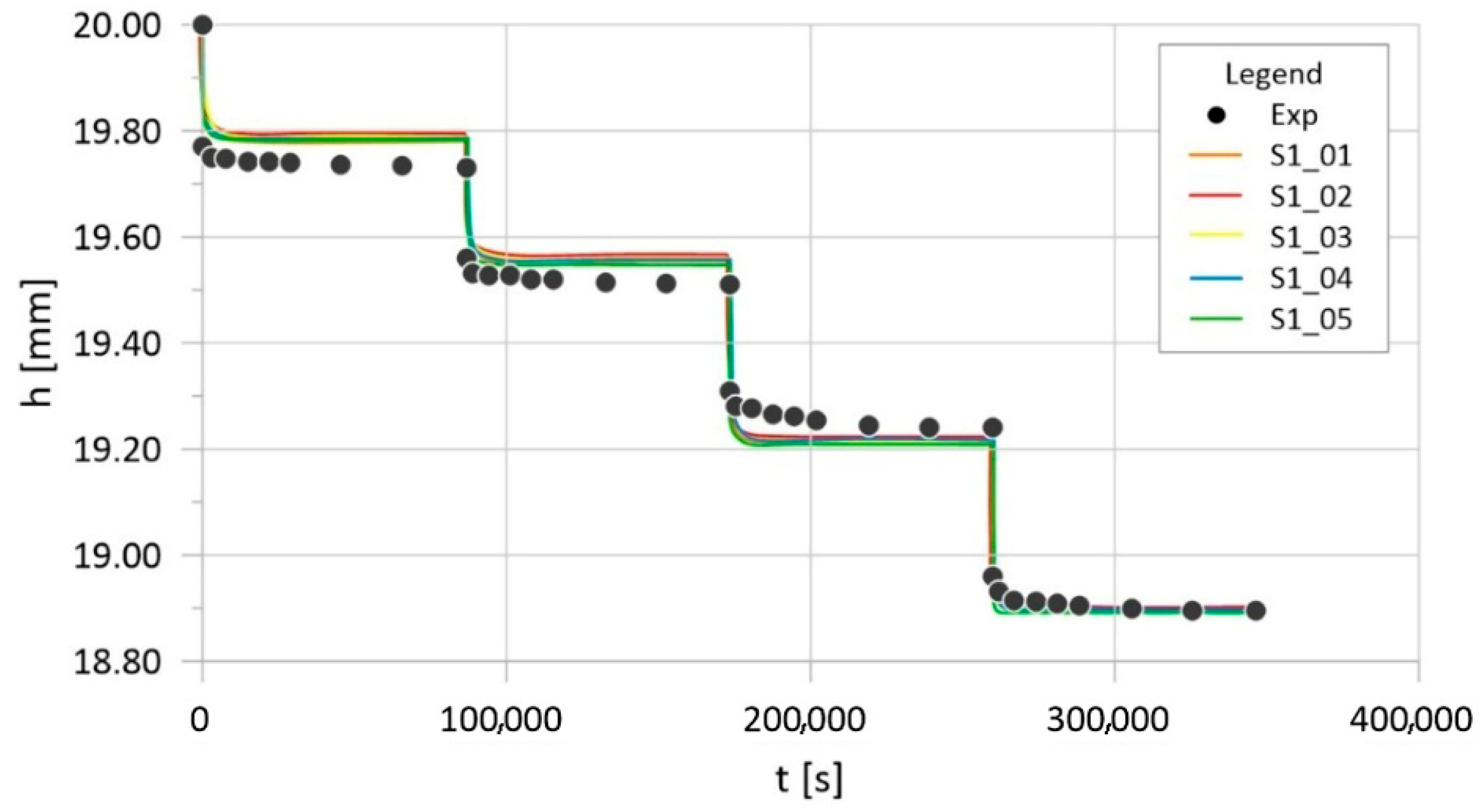
The simulation results presented in Figure 6 for the first five calibration results of stage 2 corroborate good agreement with the experimental results, regardless of the differences in the obtained parameter values.
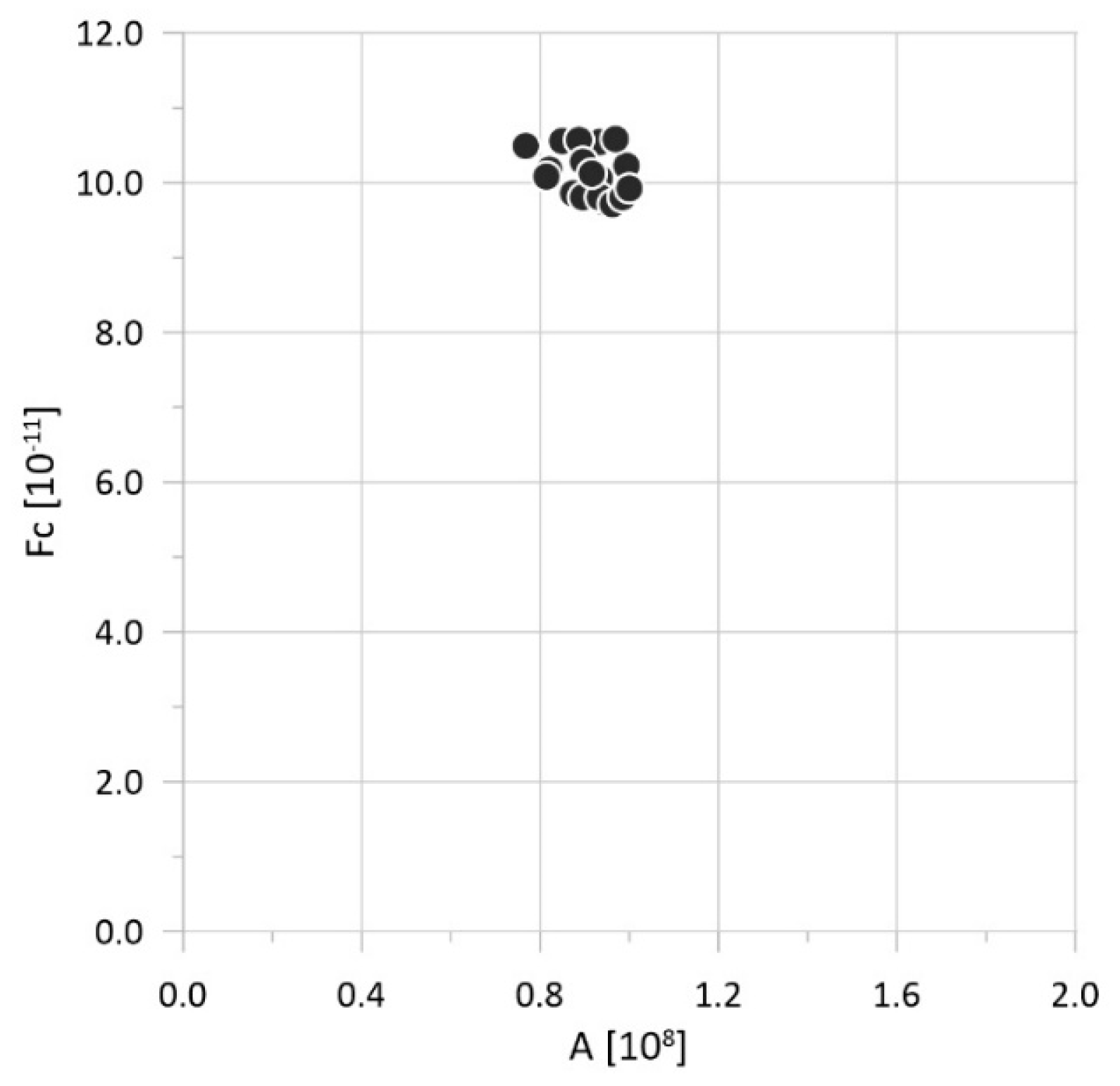
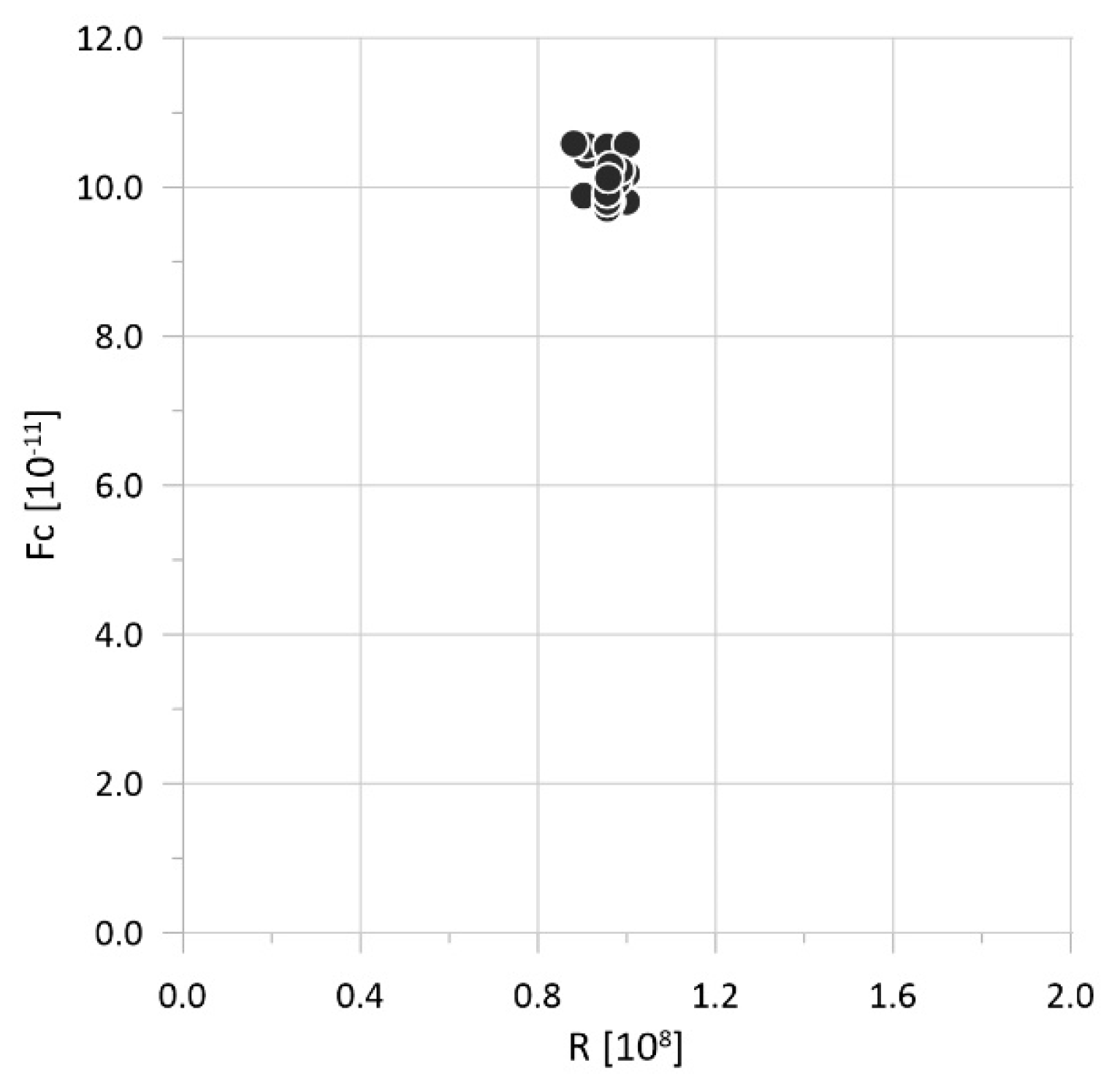
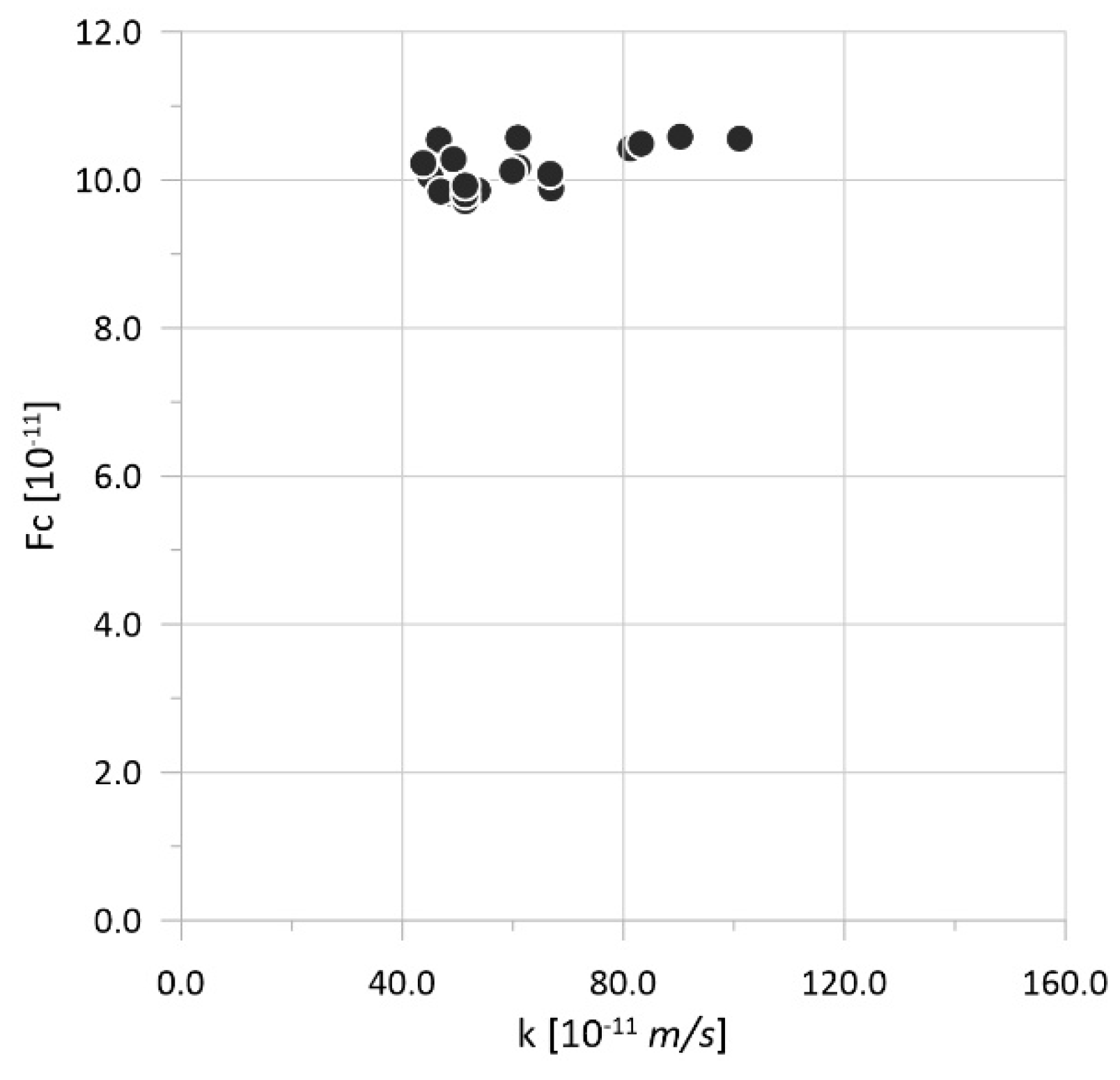
Since this is a coupled estimation of three parameters, the dependencies between parameter values and objective function values are also interesting. The dependencies are shown in Figure 7, Figure 8 and Figure 9. The results correspond to the best outcomes of each of the 20 calibrations in stage 2, where “best” refers to the parameter sets that produced the minimum value of the objective function in each calibration run.
In Figure 7, Figure 8 and Figure 9, the values on the horizontal axes in the diagrams approximately coincide with the adopted search range. The diagrams clearly indicate the multidimensional character of the dependencies and at the same time reveal the high calibration repeatability achieved.
The repeatability and convergence observed in our results are consistent with recent advancements in the use of genetic algorithms for inverse modeling tasks. In particular, improvements in genetic operator design, such as adaptive selection and crossover strategies, have been shown to enhance optimization performance across complex objective landscapes [23,25,26]. Furthermore, the integration of GAs with surrogate machine learning models has emerged as a promising approach to reduce computational load in similar calibration workflows [24]. These developments indicate potential directions for future refinement of our methodology, including the incorporation of learning-based prediction models to further accelerate convergence.
Additionally, the calibration methodology presented here could be benchmarked against modern numerical schemes applied to poroelasticity, such as HDG methods, which provide high accuracy in solving coupled solid–fluid problems [26]. Exploring such comparisons may offer further insight into the trade-offs between calibration flexibility and simulation precision in complex geoengineering applications. In future work, the GA-based calibration framework will be systematically benchmarked against other optimization algorithms commonly used in inverse analysis, such as the Levenberg–Marquardt method, Particle Swarm Optimization (PSO), and hybrid GA–machine learning approaches. This comparative study will allow for a quantitative assessment of convergence speed, robustness, and computational efficiency across different optimization paradigms.
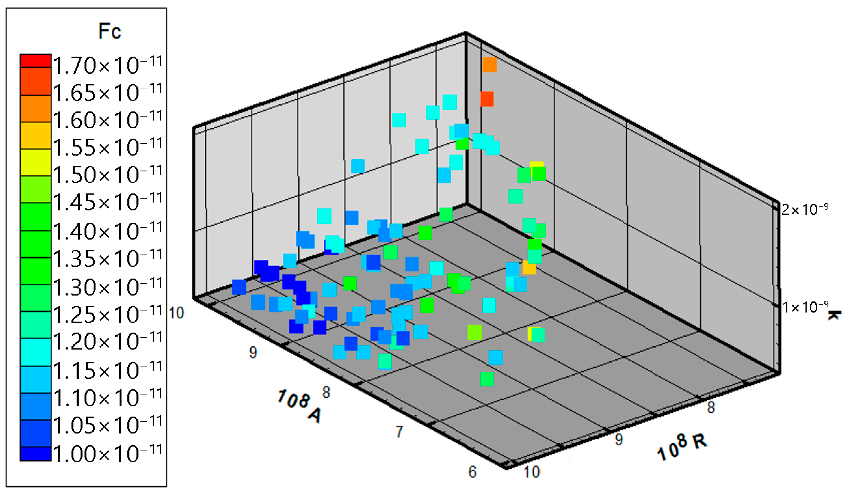
Considering that three parameters (A, R and k) were subjected to calibration, for illustrative purposes, the results can be presented in 3D. Figure 10 shows the best one hundred calibration results in the parameter space, with the points colored with the obtained objective function value. The obtained points are not uniformly distributed in space, concentrating in the region of the oblique plane defining the area towards which the highest convergence occurs.
The calibrated parameter values were also examined in terms of their physical plausibility. The obtained permeability coefficient (k ≈ 10−10–10−9 m/s) corresponds to values typical for cohesive soils and low-permeability geomaterials [21,25]. Similarly, the elastic–viscous coefficients (A ≈ 107–108 Pa and R ≈ 107–109 Pa) are consistent with the stiffness and rheological properties reported for saturated fine-grained media [27,30]. These values confirm the physical realism of the calibrated parameters and the adequacy of the GA-based optimization, which reproduced the expected consolidation response observed in the experimental oedometer tests.

6. Conclusions

This study has demonstrated the applicability of genetic algorithms for the calibration of the Biot poroelastic model in geotechnical engineering. The proposed two-stage calibration procedure, combined with an identifiability analysis, allowed us to reduce the number of calibrated parameters and improve the repeatability of the results. The obtained solutions confirmed the convergence of the GA approach, the absence of local minima, and strong agreement between numerical simulations and experimental data.
Each modification of advanced constitutive models typically requires strength tests specifically aimed at calibrating additional parameters describing the phenomenon under consideration. A similar difficulty arises when laboratory equipment makes it impossible to induce certain physical phenomena during testing. These limitations illustrate why traditional calibration approaches may be costly, time-consuming, or even infeasible in some practical cases. The results of this study confirm that reverse analysis combined with an optimizing algorithm provides an effective solution to these challenges. This approach, based on the numerical simulation of the effects of basic strength tests, enables automatic calibration of the model implemented in the computational framework. A major advantage of this approach is the ability to calibrate several numerical models using the same experimental data.
The novelty of this study lies in extending the use of genetic algorithms beyond classical geotechnical applications, such as slope stability analysis or triaxial compression test interpretation, towards the calibration of advanced poroelastic models. By applying GA-based calibration to the Biot model, which accounts for multiphase interactions and rheological effects, the methodology demonstrates advantages in addressing parameter identifiability, ensuring convergence, and improving robustness. This highlights the potential of the proposed approach for broader use in geotechnical design and analysis.
Genetic algorithms have thus been shown to be a highly effective tool that allows for automatic calibration based on simple rules. The results obtained will form the basis for further research. Therefore, this study should be regarded as a proof-of-concept for applying Genetic Algorithms to the calibration of the Biot poroelastic model, rather than as a complete identifiability study. It should also be noted that calibration and validation were performed on the same dataset, and no independent predictive validation was carried out. It should also be noted that no direct comparison with analytical consolidation solutions or formal mesh convergence studies was performed. These aspects will be addressed in future work. Moreover, the present study was based on a single oedometer test with 68 measurement points, which is insufficient for robust identifiability of multiple coupled poroelastic parameters. Full validation would require additional experiments with multiple loading paths, pore pressure measurements, and varying drainage conditions. Future work will also focus on extending the methodology to other rheological models, testing its robustness with additional experimental datasets, and exploring integration with surrogate machine learning models to further accelerate convergence and reduce computational costs. Although in this study the methodology was verified using oedometer test data, further validation with independent experimental datasets is required to fully confirm its general applicability. Future work will also include a quantitative sensitivity analysis of the Biot model parameters to complement the current qualitative identifiability assessment and to provide a more rigorous evaluation of parameter influence and model robustness. Addressing these limitations will be the subject of future research.

Author Contributions

Conceptualization, M.B.-U. and I.B.; methodology, M.B.-U.; validation, I.B.; writing—original draft preparation, M.B.-U.; writing—review and editing, I.B.; visualization, M.B.-U. and I.B. All authors have read and agreed to the published version of the manuscript.

Funding

This research received no external funding.

Institutional Review Board Statement

Not applicable.

Informed Consent Statement

Not applicable.

Data Availability Statement

The raw data supporting the conclusions of this article will be made available by the authors on request.

Conflicts of Interest

The authors declare no conflicts of interest.

References

  1. Bergkamp, E.A.; Verhoosel, C.V.; Remmers, J.J.C.; Smeulders, D.M.J. A staggered finite element procedure for the coupled Stokes–Biot system with fluid entry resistance. Comput. Geosci. 2019, 24, 1497–1522. [Google Scholar] [CrossRef]
  2. Biot, M.A. General theory of three-dimensional consolidation. J. Appl. Phys. 1941, 12, 155–164. [Google Scholar] [CrossRef]
  3. Biot, M.A. General Solutions of the Equations of Elasticity and Consolidation of a Porous Material. J. Appl. Mech. 1956, 23, 91–96. [Google Scholar] [CrossRef]
  4. Łydżba, D. Applications of the Asymptotic Homogenization Method in Soil and Rock Mechanics; Habilitation Thesis, Research Papers of the Institute of Geotechnics and Hydrotechnics Wrocław University of Technology; No. 23; Wrocław University of Technology Publishing House: Wrocław, Poland, 2002. (In Polish) [Google Scholar]
  5. Auriault, J.L. Dynamic Behavior of Porous Media. In Transport Processes in Porous Media; Springer: Dordrecht, The Netherlands, 1991; pp. 471–519. [Google Scholar]
  6. Bensoussan, A.; Lions, J.L.; Papanicolau, G. Asymptotic Analysis for Periodic Structures; North Holland Publishing Company: Amsterdam, The Netherlands, 1978. [Google Scholar]
  7. Auriault, J.L.; Sanchez Palencia, E. Etude de comportement macroscopique d’un milieu poreux sature deformable. J. Mec. 1977, 16, 575–603. [Google Scholar]
  8. Kröner, E. Effective elastic moduli of periodic and random media: A unification. Mech. Res. Commun. 1980, 7, 323–327. [Google Scholar] [CrossRef]
  9. Rubinstein, J.; Torquato, S. Flow in random porous media: Mathematical formulation, variational principles and rigorous bounds. J. Fluid Mech. 1989, 206, 25–46. [Google Scholar] [CrossRef]
  10. Auriault, J.L.; Strzelecki, T.; Bauer, J.; He, S. Porous deformable media by a very compressible fluid. Eur. J. Mech. A/Solid 1990, 9, 373–392. [Google Scholar]
  11. Uciechowska-Grakowicz, A. Temporo-Elasticity Models of a Two-Phase Medium in Mechanics of Porous Media; Strzelecki, T., Ed.; Dolnośląskie Wydawnictwo Edukacyjne: Wrocław, Poland, 2019; ISBN 978-83-7125-282-2. (In Polish) [Google Scholar]
  12. Uciechowska-Grakowicz, A.; Strzelecki, T. Application of the thermoporoelasticity model in numerical modelling of under-ground coal gasification influence on the surrounding medium. Stud. Geotech. Mech. 2021, 43, 116–1344. [Google Scholar] [CrossRef]
  13. Strzelecki, T.; Uciechowska, A. Thermal consolidation process of multiphase medium consisting of elastic skeleton, water, and water vapour. Acta Geophys. 2014, 62, 1163–1178. [Google Scholar] [CrossRef]
  14. Zhang, Q.; Yin, Z.; Yan, X. Material Constants of Anisotropic Poroelasticity and Its Impacts on Shale Gas Production. Energy Fuels 2023, 37, 18722–18734. [Google Scholar] [CrossRef]
  15. Chen, H.; Chen, Y.; Kou, J. Energy stable finite element approximations of gas flow in poroelastic media. Comput. Methods Appl. Mech. Eng. 2024, 428, 117082. [Google Scholar] [CrossRef]
  16. Bartlewska, M.; Strzelecki, T. One-dimensional consolidation of the porous medium with the Rheological Kelvin-Voight skeleton. Stud. Geotech. Mech. 2008, 30, 115–122. [Google Scholar]
  17. Bartlewska, M.; Strzelecki, T. Equations of Biot’s consolidation with Kelvin-Voight rheological frame. Stud. Geotech. Mech. 2009, 30, 3–15. [Google Scholar]
  18. Terzaghi, K. Theoretical Soil Mechanics; Wiley: New York, NY, USA, 1943. [Google Scholar]
  19. Wood, D.M. Soil Behaviour and Critical State Soil Mechanics; Cambridge University Press: Cambridge, UK, 1990. [Google Scholar]
  20. Atkinson, J. The Mechanics of Soils and Foundations, 2nd ed.; CRC Press: London, UK, 2007. [Google Scholar]
  21. Hashash, Y.M.A.; Yao, J.I.C. Calibration of soil constitutive models for numerical analysis in geotechnical engineering. Soil Dyn. Earthq. Eng. 2005, 25, 789–798. [Google Scholar] [CrossRef]
  22. Brinkgreve, R.B.J. Selection of soil models and parameters for geotechnical engineering application. In Proceedings of the PLAXIS Symposium, Paris, France, 1 August 2002; pp. 69–98. [Google Scholar]
  23. Huang, T.; Yin, H.; Huang, X. Improved genetic algorithm for multi-threshold optimization in digital pathology image segmentation. Sci. Rep. 2024, 14, 22454. [Google Scholar] [CrossRef]
  24. Kneiding, P.; Balcells, M. Augmenting genetic algorithms with machine learning for inverse molecular design. Chem. Sci. 2024, 15, 5831–5843. [Google Scholar] [CrossRef]
  25. Robson, J.D.; Armstrong, D.; Cordell, J.; Pope, D.; Flint, T.F. Calibration of constitutive models using genetic algorithms. Mech. Mater. 2024, 189, 104881. [Google Scholar] [CrossRef]
  26. Meddahi, S. hp Error Analysis of HDG for Dynamic Poroelasticity. arXiv 2025, arXiv:2503.08360. [Google Scholar] [CrossRef]
  27. Bartlewska-Urban, M.; Strzelecki, T.; Urban, R. Determination of effective parameters of Biot model with the Kelvin–Voight rheological skeleton. Arch. Civ. Mech. Eng. 2015, 15, 1173–1179. [Google Scholar] [CrossRef]
  28. Biot, M.A.; Willis, D.G. The Elastic Coefficients of the Theory of Consolidations. J. Appl. Mech. 1957, 24, 594–601. [Google Scholar] [CrossRef]
  29. Coussy, O. Mechanics and Physics of Porous Solids; John Wiley & Sons: Hoboken, NJ, USA, 2011; ISBN 978-1-119-95616-7. [Google Scholar]
  30. Ma, Y.; Chen, X.H.; Yu, H.S. An extension of Biot’s theory with molecular influence based on mixture coupling theory: Mathematical model. Int. J. Solids Struct. 2020, 191–192, 76–86. [Google Scholar] [CrossRef]
  31. Srokosz, P. Selected Applications of Genetic Algorithms in Geotechnics; Wydawnictwo UWM: Olsztyn, Poland, 2012; ISBN 8372997608. (In Polish) [Google Scholar]
  32. Borregales, M.A.; Kumar, K.; Nordbotten, J.M.; Radu, F.A. Iterative solvers for Biot model under small and large deformations. Comput. Geosci. 2020, 25, 687–699. [Google Scholar] [CrossRef]
  33. Kozubal, J.V.; Kania, T.; Tarawneh, A.S.; Hassanat, A.; Lawal, R. Ultrasonic assessment of cement-stabilized soils: Deep learning experimental results. Measurement 2023, 223, 113793. [Google Scholar] [CrossRef]
  34. Martínez López, Y.; Oquendo Ferrer, H.; Caballero Mota, Y.; Guerra-Rodríguez, L.E.; Junco-Villegas, R.; Benítez Cortés, I.; Madera Quintana, J. Aplicación de la investigación de operaciones a la distribución de recursos relacionados con la COVID-19. Retos Dir. 2020, 14, 86–105. [Google Scholar]
  35. Amawi, R.M.; Al-Hussaeni, K.; Keeriath, J.J.; Ashmawy, N.S. A Machine Learning Approach to Evaluating the Impact of Natural Oils on Alzheimer’s Disease Progression. Appl. Sci. 2024, 14, 6395. [Google Scholar] [CrossRef]
  36. Han, J. CNN-Based Multi-Factor Authentication System for Mobile Devices Using Faces and Passwords. Appl. Sci. 2024, 14, 5019. [Google Scholar] [CrossRef]
  37. Villa-Pérez, M.E.; Alvarez-Carmona, M.A.; Loyola-González, O.; Medina-Pérez, M.A.; Velazco-Rossell, J.C.; Choo, K.K.R. Semi-supervised anomaly detection algorithms: A comparative summary and future research directions. Knowl.-Based Syst. 2021, 218, 106878. [Google Scholar] [CrossRef]
  38. Kramer, O.; Kramer, O. Genetic Algorithms; Springer International Publishing: Berlin/Heidelberg, Germany, 2017. [Google Scholar] [CrossRef]
  39. Forrest, S. Genetic algorithms. ACM Comput. Surv. CSUR. 1996, 28, 77–80. [Google Scholar] [CrossRef]
  40. Holland, J.H. Adaptation in Natural and Artificial Systems; University of Michigan Press: Ann Arbor, MI, USA, 1975. [Google Scholar]
  41. Goldberg, D.E. Genetic Algorithms in Search, Optimization, and Machine Learning; Addison-Wesley: Boston, MA, USA, 1989. [Google Scholar]
  42. Mitchell, M. An Introduction to Genetic Algorithms; MIT Press: Cambridge, MA, USA, 1996. [Google Scholar]
  43. Forrest, S. Genetic algorithms: Principles of natural selection applied to computation. Science 1993, 261, 872–878. [Google Scholar] [CrossRef]
  44. Kramer, O. Genetic Algorithm Essentials; Springer: Cham, Switzerland, 2017. [Google Scholar]
  45. Rutkowski, L. Computational Intelligence: Methods and Techniques; Springer Science & Business Media: Berlin/Heidelberg, Germany, 2008; ISBN 978-3540762874. [Google Scholar]
  46. Whitley, D. A genetic algorithm tutorial. Stat. Comput. 1994, 4, 65–85. [Google Scholar] [CrossRef]
  47. Baker, J.E. Adaptive selection methods for genetic algorithms. In Proceedings of the 1st International Conference on Genetic Algorithms, Broadway Hillsdale, NJ, USA, 1 July 1985; pp. 101–111. [Google Scholar]
  48. Haupt, R.L.; Haupt, S.E. Practical Genetic Algorithms; Wiley-Interscience: Hoboken, NJ, USA, 2004. [Google Scholar]
  49. PDE Solutions Inc. FlexPDE 6: A Flexible Solution for Partial Differential Equations. Available online: https://www.pdesolutions.com (accessed on 12 October 2025).
  50. Mo, X.; Zhang, D.; Ge, F.; Huang, H.; Chen, C.; Liu, M.; Chen, H. A P-THMC Model to Solidification and Solute Separation in Saturated Freezing Soil. Water Resour. Res. 2025, 61, e2024WR038885. [Google Scholar] [CrossRef]
  51. Kozeny, J. Über Kapillare Leitung des Wassers im Boden; Sitzungsberichte der Akademie der Wissenschaften: Vienna, Austria, 1927; pp. 136, 271–306. [Google Scholar]
  52. Carman, P.C. Fluid flow through granular beds. Trans. Inst. Chem. Eng. 1937, 15, 150–166. [Google Scholar] [CrossRef]
  53. Carman, P.C. Flow of Gases Through Porous Media; Butterworths Scientific Publications: London, UK, 1956. [Google Scholar]
  54. ASTM D2435; Standard Test Methods for One-Dimensional Consolidation Properties of Soils Using Incremental Loading. ASTM: West Conshohocken, PA, USA, 2011.
  55. Walter, E.; Pronzato, L. Identification of Parametric Models from Experimental Data; Springer: Berlin, Germany, 1997. [Google Scholar]
  56. Brun, R.; Reichert, P.; Künsch, H.R. Practical identifiability analysis of large environmental simulation models. Water Resour. Res. 2001, 37, 1015–1030. [Google Scholar] [CrossRef]
  57. Dana, S.; Wheeler, M.F. Convergence analysis of fixed stress split iterative scheme for anisotropic poroelasticity with tensor Biot parameter. Comput. Geosci. 2019, 22, 1219–1230. [Google Scholar] [CrossRef]
  58. Li, S.J.; Shao, L.T.; Wang, J.Z.; Liu, Y.X. Inverse procedure for determining model parameter of soils using real-coded genetic algorithm. J. Cent. South Univ. 2012, 19, 1764–1770. [Google Scholar] [CrossRef]
  59. Moufida, M. Identification of soil mechanical parameters by inverse analysis using genetic algorithm and hybrid methods. Slovak J. Civ. Eng. 2022, 17, 1–12. [Google Scholar]
  60. Antonietti, P.F.; Bonetti, S.; Botti, M. Discontinuous Galerkin approximation of the fully-coupled thermo-poroelastic problem. SIAM J. Sci. Comput. 2023, 45, A621–A645. [Google Scholar] [CrossRef]
  61. Çeşmelioğlu, A.; Lee, J.J.; Rhebergen, S. Analysis of an embedded-hybridizable discontinuous Galerkin method for Biot’s consolidation model. J. Sci. Comput. 2023, 97, 1–26. [Google Scholar] [CrossRef]
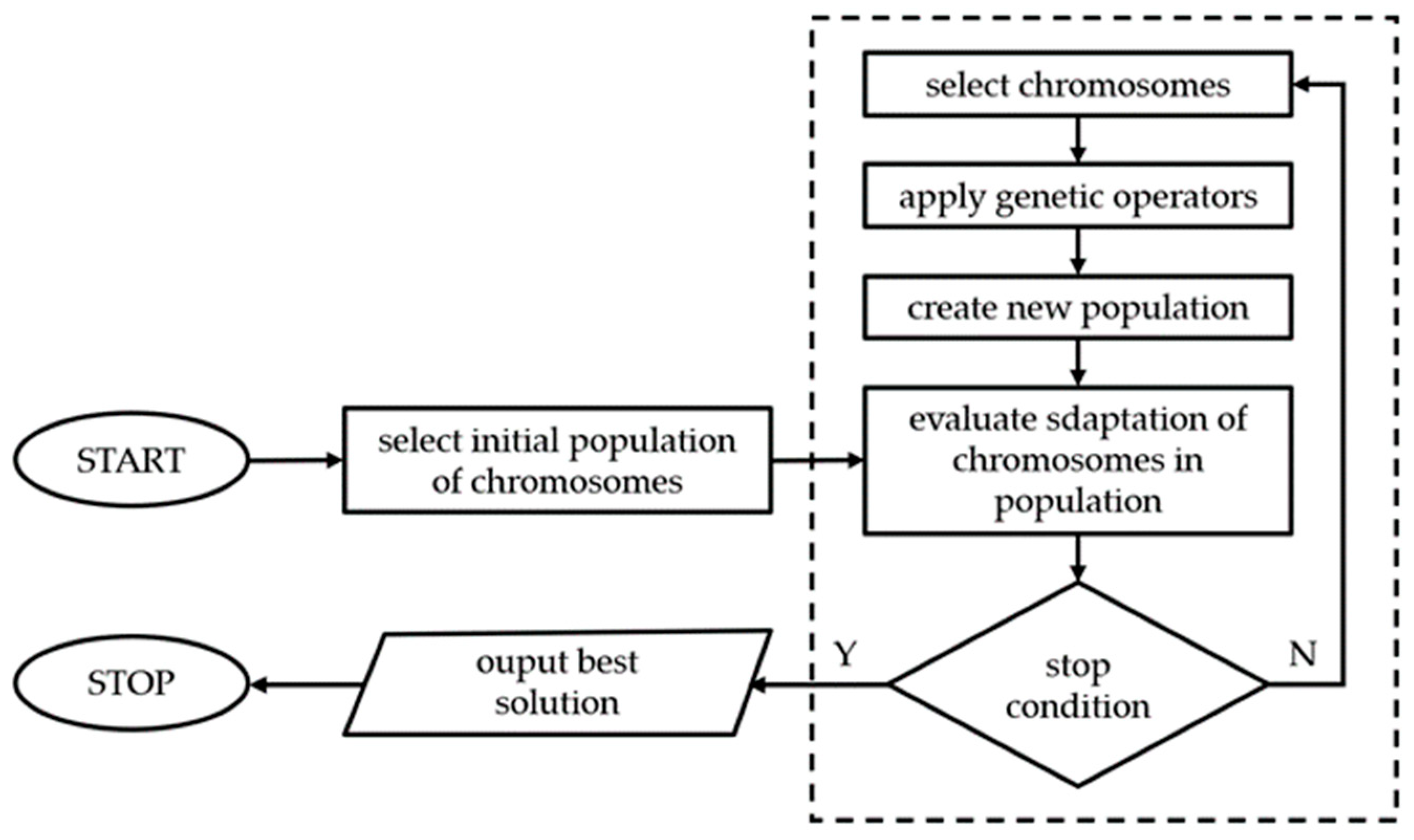
Figure 1. Flowchart of the general workflow of a genetic algorithm.
Applsci 15 11972 g001
Figure 3. Principle of the operation of mutation operator.
Applsci 15 11972 g003
Figure 4. The successive changes in sample height correspond to the successive changes in load.
Applsci 15 11972 g004
Figure 5. Simulation results for selected results of stage 1.
Applsci 15 11972 g005
Figure 6. Simulation results for selected results of stage 2.
Applsci 15 11972 g006
Figure 7. Dependence between the objective function (Fc) and parameter A. The black dots represent the objective function values obtained for individual parameter candidates during the calibration process.
Applsci 15 11972 g007
Figure 8. Dependence between the objective function (Fc) and parameter R. The black dots represent the objective function values obtained for individual parameter candidates during the calibration process.
Applsci 15 11972 g008
Figure 9. Dependence between the objective function (Fc) and parameter k. The black dots represent the objective function values obtained for individual parameter candidates during the calibration process.
Applsci 15 11972 g009
Figure 10. Best 100 calibration results in the parameter space (A, R, k) from stage 2. Color scale represents the objective function Fc values [10−11], confirming high convergence and repeatability.
Applsci 15 11972 g010
Table 1. Physical interpretation of Biot model parameters.
ParameterPhysical MeaningUnitTypical RangeReference
NBulk modulus of the porous skeleton (elastic compressibility of the solid phase)Pa106–108[2,27]
AShear modulus of the skeleton (resistance to shear deformation)Pa107–108[28,29]
RBulk modulus of pore fluidPa107–109[3,29]
HSolid–fluid coupling modulus (interaction between phases)Pa107–109[3,27]
kDarcy permeability coefficientm/s10−11–10−9[21,30]
Table 2. Ranges of calibrated parameters.
ParameterMinMaxThe Estimation
Accuracy
N [Pa]1 × 1061 × 1087
A [Pa]1 × 1071 × 1087
R [Pa]1 × 1071 × 1097
H [Pa]1 × 1071 × 1097
k [m/s]1 × 10−111 × 10−910
Table 3. Calibration results for all parameters—stage 1.
NumN
[107 Pa]
A
[108 Pa]
R
[108 Pa]
H
[108 Pa]
k
[10−11 m/s]
Fc
[108]
Δ
[mm]
11.3871.8201.4020.69814.429.910.038
21.2521.7760.2940.14591.079.420.037
31.8350.5341.6860.92382.7011.440.041
41.4611.9700.4890.26536.019.780.038
51.2521.1471.5810.54912.289.900.038
61.5811.3871.6710.7284.509.440.037
71.8501.0281.6260.92338.5410.300.039
81.0280.6681.0720.2507.429.820.038
90.3991.8200.5340.14539.329.430.037
101.4021.0871.2370.4447.039.820.038
111.9402.0000.4890.41426.689.480.037
121.8201.6411.6261.02834.079.900.038
131.9101.1771.4910.89331.359.590.038
141.4610.8631.4610.56427.6510.450.039
151.0281.5811.3870.54948.2710.960.040
161.1471.4611.6110.5648.599.360.037
171.2071.9100.5790.26516.958.960.036
181.0131.8351.5210.62430.189.990.038
181.7461.8501.4910.93824.5410.200.039
190.9681.5211.1470.44453.9110.740.040
201.3841.4541.2200.56731.779.940.038
Avg0.3900.4360.4600.26922.90.5850.001
SD1.3871.8201.4020.69814.429.910.038
Table 4. Calibration results for selected parameters—stage 2.
NumA
[108 Pa]
R
[108 Pa]
k
[10−11 m/s]
Fc
[108]
Δ
[mm]
10.9030.91081.3410.430.039
20.8730.99353.729.860.038
30.8951.00047.699.810.038
40.9700.90366.949.890.038
50.9480.95551.389.730.038
60.7680.98583.2810.490.039
70.9330.95544.9610.060.038
80.8211.00060.9110.180.039
90.8130.97866.7510.090.039
100.9330.96349.249.810.038
110.9630.95551.389.710.038
120.8500.910100.9910.560.039
130.9930.95546.919.840.038
140.9330.95546.5210.540.039
150.8881.00060.9110.570.039
160.9930.98543.8010.230.039
170.8950.96349.2410.280.039
180.9850.95551.389.800.038
181.0000.95551.389.920.038
190.9700.88090.2910.580.039
200.9160.95859.9510.120.039
Avg0.0640.03316.200.310.001
SD0.9030.91081.3410.430.039
Disclaimer/Publisher’s Note: The statements, opinions and data contained in all publications are solely those of the individual author(s) and contributor(s) and not of MDPI and/or the editor(s). MDPI and/or the editor(s) disclaim responsibility for any injury to people or property resulting from any ideas, methods, instructions or products referred to in the content.