Abstract
This study presents an analysis of transverse vibration behavior of a fluid-conveying pipe mounted on an elastic foundation, incorporating both classical analytical techniques and modern physics-informed neural network (PINN) methodologies. A partial differential equation (PDE) architecture is developed to approximate the solution by embedding the physics PDE, initial, and boundary conditions directly into the loss function of a deep neural network. A one-dimensional fourth-order PDE is employed to model governing transverse displacement derived from Euler–Bernoulli beam theory, with additional terms representing fluid inertia, flow-induced excitation, and stochastic force modelled as Gaussian white noise. The governing PDE is decomposed via separation of variables into spatial and temporal components, and modal analysis is employed to determine the natural frequencies and mode shapes under free–free boundary conditions. The influence of varying flow velocities and excitation frequencies on critical buckling behavior and mode shape deformation is analyzed. The network is trained using the Resilient Backpropagation (RProp) optimizer. A preliminary validation study is presented in which a baseline PINN is benchmarked against analytical modal solutions for a fluid-conveying pipe on an elastic foundation under deterministic excitation. The results demonstrate the capability of PINNs to accurately capture complex vibrational phenomena, offering a robust framework for data-driven modelling of fluid–structure interactions in engineering applications.
1. Introduction
Modal analysis and fluid-induced transverse vibration in pipes on elastic foundations are complex phenomena influenced by various factors, including pipe geometry, fluid velocity, boundary conditions, and the characteristics of the foundation. The natural frequency of a pipe, crucial for predicting and mitigating vibration issues, can be estimated using simplified models that relate the pipe’s geometry to a Euler–Bernoulli beam with correction factors for different boundary conditions, as demonstrated in studies using ANSYS simulations and experimental verifications [1]. The dynamics of fluid-conveying pipes, particularly those with non-linear geometries like L-shaped pipes, are significantly affected by fluid velocity, which reduces natural frequencies and alters modal shapes, especially at critical velocities where modal combinations occur [2]. Fluid–structure interaction further complicates the modal analysis, as seen in high-pressure environments where the interaction reduces natural frequencies and increases displacement due to the dynamic loads [3,4,5,6,7]. The impact of elastic foundations, such as Winkler, Pasternak, and Hetényi types, on the vibrational behavior of pipes is profound, with foundation stiffness and type affecting the natural frequencies and stability of the system [8,9,10]. Specifically, a two-parameter foundation can enhance both the vibration frequency and critical velocity, thereby improving stability [11]. Nonlinear vibration analysis of fluid-conveying anisotropic laminated tubular beams on elastic foundations reveals that boundary conditions, geometric imperfections, and foundation characteristics significantly influence dynamic behavior [12]. Additionally, the stability and nonlinear vibration characteristics of composite pipes are affected by factors such as viscoelastic coefficients and fiber orientation, with elastic boundary conditions playing a critical role in determining the system’s stability and critical velocities [13]. Physics-informed neural networks (PINNs) have emerged as a powerful tool for analysing the vibration of pipes, offering a promising alternative to traditional numerical methods. The application of PINNs in this context involves solving the partial differential equations (PDEs) governing the dynamic behavior of pipes, which are often complex due to factors such as flow-induced vibrations and the elastic properties of the foundation. The integration of PINNs with advanced techniques, such as Fourier feature mapping, helps overcome the spectral bias problem, enabling accurate modelling of both low- and high-frequency vibrations in pipelines, as demonstrated by Ting Zhang et al. [14]. The use of PINNs in flow-induced vibration scenarios, as explored by Guang Yin et al., shows their capability in predicting complex flow fields around vibrating structures, which is essential for subsea pipeline applications [15]. The advanced time-marching PINN (AT-PINN) approach developed by Zhaolin Chen et al. further enhances the accuracy and efficiency of long-duration simulations, addressing the challenges of accumulative error and computational cost [16]. Additionally, the incorporation of strategies like multiscale Fourier feature mapping and frequency transferring, as discussed by Xintao Chai et al., improves the representation of high-frequency components, which is critical for accurate vibration analysis [17]. Recent studies have focused on enhancing the accuracy and robustness of PINNs for complex fluid–structure interactions, including cantilever dynamics and high-order differential operators [18]. Innovations such as integrating residual networks (ResNet) into PINN architectures improve training stability and the capacity to capture complex flow dynamics, mitigating vanishing or exploding gradients [19]. Furthermore, adaptive-weight PINNs (AW-PINNs) have been developed to balance the training rates of distinct loss terms, yielding significant gains in prediction accuracy and robustness [20]. Validation spans multiple case studies, including flow around cylinders and VIV scenarios, where improved PINNs deliver results comparable to or better than conventional computational fluid dynamics (CFD), with different computational trade-offs [21,22]. Deep neural networks (DNNs) have also been applied to predict dynamic responses in systems like the VIVACE converter, which harnesses vortex-induced vibrations (VIVs) for energy conversion, demonstrating good agreement with experimental data and potential for reducing experimental efforts [23]. In contrast, convolutional neural networks (CNNs) have been employed for classifying vibration states and flow patterns in pipelines, with applications ranging from vibration-induced fatigue risk assessment to flow pattern identification in multiphase flows [24,25]. The evolution of PINNs continues to expand the toolkit for fluid dynamics simulation, offering a more efficient and potentially more accurate route for solving complex fluid-induced vibration problems [26,27].
Despite numerous studies on the vibration of fluid-conveying pipes, limited attention has been given to systems under free-tension conditions, interacting with elastic foundations and subjected to stochastic excitation. Moreover, traditional numerical approaches often face difficulties in accurately capturing the nonlinear dynamics arising from Coriolis and centrifugal effects, especially in data-sparse scenarios. Early foundations established PINNs for forward and inverse PDE problems, enabling data assimilation with physical regularizations. Subsequent studies targeted structural vibration over long time windows with advanced time-marching PINNs that control cumulative error. Parallel to the PINN advances, recent mechanics studies continued to map stability boundaries for fluid-conveying pipes on elastic foundations, especially Winkler-type foundation supports, which is adopted as the baseline physics presented in this study. Prior work has shown that PINNs can (i) learn vibration fields with limited measurements, (ii) handle moderately broadband responses when frequency features are encoded, and (iii) extend to longer horizons with time-marching strategies. Key open challenges remain, such as spectral bias that suppresses high-frequency content, stiffness and multiscale coupling from Coriolis terms and foundation reactions, accumulation of error in long integrations, and robustness under measurement noise. This study aims to address limitations of classical solvers, a PINN is implemented to approximate the solution of the governing PDE, embedding physical laws directly into the training process. The PINN framework encodes the governing PDE and boundary conditions inside the loss, which functions as a physics-based prior and allows training with few measured points. A physics-informed neural network is trained on the governing free-tension pipe–fluid PDE on a Winkler foundation with Coriolis and centrifugal couplings and evaluated against the analytical solution. Architecture, training curves, regression results, and FFT agreement collectively substantiate the robustness of the proposed hybrid approach, which enables improved modelling accuracy and computational efficiency.
2. Mathematical Model of Pipe Fluid Flow-Induced Vibration
The proposed model describes essential concepts in the dynamics analysis of the pipe system embedded on an elastic foundation. It integrates the necessary mathematics methodologies and mechanical system fundamentals into a framework by recognizing and isolating structural and systematic deployment and realistic application of physical principles. It is possible for fluid flowing through a pipe to exert pressure on the walls of the pipe, causing the pipe to be deflected. Pipe whip is the dynamic response of a pipeline to an instantaneous rupture. There is also the possibility of a steady flow deflecting a pipe. A thin-walled pipe can vibrate at high amplitude when a high-velocity flow passes through it. The dynamical behavior of a fluid-conveying pipe is highly dependent on the support conditions of the pipe as well as variations in the flow velocity. Despite small transverse deflections, the pipe retains its geometrical properties under inviscid and incompressible fluid. A pipe span with a transverse deflection w(x,t) from equilibrium is shown in Figure 1.
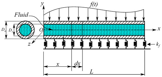
Figure 1.
Model of a fluid-conveying pipe resting on elastic foundation.
The fluid-conveying pipe’s motion equation on a one-parameter foundation is derived using classical beam theory assumptions and is detailed as follows:
- There is linear elastic behavior, homogeneity and isotropy in the pipe and soil materials;
- In comparison with the pipe thickness, the displacements are small;
- When compared with unity, the axial strain is small;
- Shear stresses and normal transversal strains are negligible;
- As a result of the Euler–Bernoulli hypothesis, the cross-sections are plane and perpendicular.
In the scenario described, fluid flows through a pipe with a constant velocity (v) and pressure (p). The pipe has a certain length (L), modulus of elasticity (E), and moment of inertia (I). Figure 2 shows a fluid element separated from the pipe to improve clarity and Figure 3 shows smaller elements cut from the pipe. As the pipe deflects, the fluid experiences centrifugal acceleration. In addition, the pipe walls apply a pressure force (N per unit length) to the fluid element, which opposes the accelerations caused by the changing curvature of the pipe. The combination of these forces, along with the mechanical properties of the pipe, will affect the behavior of the system and the fluid flowing through it.
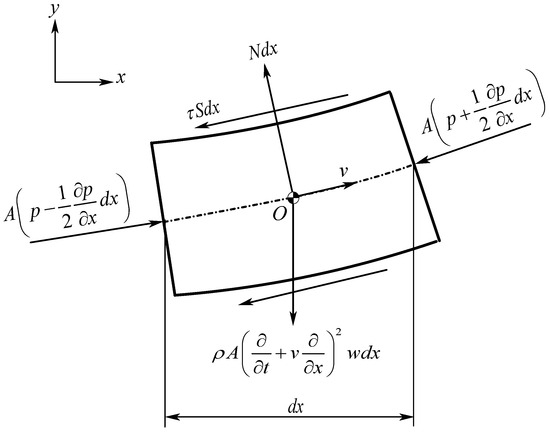
Figure 2.
Deformable moving control volume of the fluid differential element.
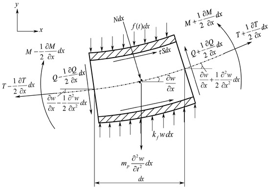
Figure 3.
Forces and moments acting on the deformed pipe differential element on elastic foundation.
The forces in the y-direction are balanced during small fluid element deformations.
Flow friction resists pressure gradient along the pipe. Figure 2 illustrates constant flow velocity by summing forces parallel to the pipe axis. Where S represents the longitudinal inner perimeter of the pipe, τ denotes the transverse shear stress on the inner pipe surface.
The equations that describe the motion of the pipe along its length axis are obtained by calculating the total force along the length of the pipe. This approach is illustrated through the force balance equation, depicted by the algebraic summation of forces along the pipe axis, as shown in Figure 3. A similar approach was also employed by researchers in related studies to address vibrations induced by internal fluid flow [28,29].
The equation in question represents the motion of a pipe element transversely. That equation basically states that Q, the transverse shear force, and T, the longitudinal tension, create acceleration in the y-direction, perpendicular to the pipe axis, for the pipe under small deformations where mp is the mass of the pipe per unit length when is empty. A pipe element that is subjected to a transverse resistance force has a transverse shear stress Q variable, with a maximum on the neutral axis, and has undergone a bending moment M in a deformed pipe element expressed as
Given that Q exhibits a proportional relationship with ∂3w/∂x3, the third term on the left-hand side of Equation (3) is characterized by an order of w2 and is therefore disregarded in the context of linear small-deformation analysis. Equations (1), (4) and (5) are combined in such a way as to elimination of both F and Q.
The shear stress τ is eliminated from (2) and (3) to give
The condition of the flow is steady-state, indicating that the difference between pA and T is constant along the pipe’s span. When assuming that the tension in the pipe is zero at the end, and the fluid pressure inside the pipe is equal to the surrounding pressure p = T = 0 at x = L, then (7) implies that pA − T = 0 for all x. If the pipe is fitted with a converging nozzle, taking into account momentum gives pA − T = pAv(vj − v), where vj is the throat velocity. Using (6), substituting pA − T = 0. Algebraic manipulation of the deformed movable control volume of the fluid differential element in Figure 2 and forces and moments acting on the deformed pipe differential element on elastic foundation in Figure 3 yield the equation of motion of a pipe free-tension transverse vibration conveying fluid expressed as
where ρA + mp represents the mass per unit length of the pipe and fluid in the pipe.
Equation (8) accounts for elastic, centrifugal, Coriolis, inertia, elastic resistance and random excitation. The characteristic of the elastic foundation is conceptualized as a Winkler-type foundation. The boundary conditions that pertain to a free–free pipe that is supported by an elastic foundation are:
The first term of Equation (8) represents the elastic force is the disproportionate force, which is caused by the deformation of the pipe. This causes the natural frequency to decrease and eventually buckle. The fourth and the fifth terms refer to inertia force and elastic resistance due to the Winkler foundation which are all independent of flow. The second term accounts for the force that’s caused by the movement of fluid through a curved path (centrifugal force). The third term from the left is the force required to rotate fluid elements with the pipe’s local rotation referred as a Coriolis force. It causes an asymmetric alteration of classical mode shapes, resulting in flutelike instability due to the mixed derivative. It also makes (8) difficult to solve. The force f(t) right-hand side of (8) represents non-conservative random force per unit length characterized by Gaussian white noise. Gaussian white noise can be characterized as a random process given by a Gaussian probability distribution with zero mean.
A joint Gaussian distribution represents a specific category of two-dimensional probability distribution in which two random variables are distributed together and adhere to a Gaussian (normal) distribution framework. This implies that the Probability Density Function (PDF) corresponding to the joint distribution can be articulated through the multivariate normal distribution PDF. Specifically, if x and y denote a pair of two random variables exhibiting a joint Gaussian distribution, then their joint PDF can be articulated as:
In the context of statistical analysis, the parameters μx and μγ denote the means, while σx and σγ represent the standard deviations of the random variables x and y, respectively. The symbol κ denotes the correlation coefficient between x and y. The joint Gaussian distribution is widely used across various scientific disciplines, including physics, engineering, and finance, owing to its advantageous mathematical properties. Furthermore, Equation (8) does not exhibit classical normal modes. Instead, it permits a separable representation, whereby the solution can be expressed as the product of a spatial function, (x), and a temporal function, ϕ(t) corresponding to the spatial and temporal components. This leads to a formulation of the solution in the separable form:
Substituting (13) into (8), the equation of transverse vibration conveying fluid can be rewritten in the separate the spatial and temporal terms:
where λ is the separation constant that decouples the spatial and temporal parts into two independent equations. In spatial (14) acts as an eigenvalue in this equation, determining the allowable mode shapes and temporal (15) represents the critical load required to maintain stability (buckling). The general solution for (x) is a linear combination of the eigenfunctions and can be expressed as:
where C1, C2, C3 and C4 are constant that are determined by Free–Free boundary conditions (9) and (10), the shear force and bending moment are vanishing at ends of the pipe:
After applying the boundary conditions and algebraic manipulations, Equation (17) can be rearranged and expressed in a matrix form:
The non-trivial frequency equation, which represents the condition necessary to determine the natural frequencies of the pipe system under the Free–Free boundary conditions, can be derived and expressed in the following form:
The transcendental Equation (19) has infinite solutions and can be numerically solved; the first five numbers are presented in Table 1 below:

Table 1.
Five knL numerical solutions.
The normal function of the pipe span shown in Figure 1 and given by free–free boundary conditions (9) and (10) satisfies the mode shapes corresponding to the natural frequencies. The spatial solution of (19) representing the normal modes of pipe oscillation can be written as:
The natural frequency of a pipe corresponds to the specific spatial wavenumbers kn = nπ/L (for boundary conditions) in the influence of fluid flow, also known as the circular fundamental frequency, can be represented mathematically using the following equation:
The velocity at which the bending waves travel through the pipe, also known as phase velocity, is represented by
The critical velocity of flow-induced vibration that results in buckling is often associated with the occurrence of a critical flow rate or turbulent flow. It occurs when fluid flows through a pipe and exerts a force on the walls of the pipe causing compressive stress induced by exceeding the critical buckling stress of the pipe material. The stiffness of the pipe is directly proportional to the external diameter Do, because it reflects the resistance of the pipe to bending and buckling and directly influences the interaction of the pipe with external forces, supports, and foundations. The compressive stress induced by fluid flow in the pipe walls must not exceed the material’s critical buckling stress:
The critical velocity at which the system transitions from stability to instability is associated with the onset of buckling in the pipe. The phenomenon occurs when the destabilizing forces induced by the fluid flow surpass the restoring forces provided by the stiffness of the pipe and the elastic foundation. The critical velocity, corresponding to the condition where the eigenvalue of the system leads to instability, can be expressed as:
Table 2 summarizes the geometric, material, and foundation parameters for the pipe system model, including pipe dimensions, fluid properties, structural stiffness and density, and soil constants. The consolidated set establishes the baseline coefficients in the governing mass, damping, and stiffness operators and material designations.
Table 2.
Material and fluid properties.
3. Normal Vibration Modes in Pipe System Under No-Flow Condition
In the analysis of the dynamic behaviour of a pipe system, understanding the normal vibration modes is essential as they form the basis for characterizing the response of the system under various excitations. The normal modes represent the distinct patterns in which the system oscillates naturally, each associated with a specific frequency and shape. These modes are particularly relevant in systems without fluid flow, where structural dynamics dominate. Gaussian white noise enters as an additive broadband force, leading after separation in Equation (15) to modal responses that act as linear filters. The white-noise does not by itself move the deterministic stability boundary; rather, it amplifies the structure’s frequencies. Raising the Winkler foundation stiffness kf in Equations (8) and (14) counters that effect by shifting modal peaks upward and reducing low-frequency amplification.
Figure 4a shows a typical five normal transversal vibration modes of the pipe without fluid flow. It is noted that five modes of vibration are considered, and the higher-order vibration modes are ignored because they behave similarly to the first two modes. It is evident that each normal mode vibrates progressively with a different shape and frequencies. Figure 4b illustrates the relationship between velocity and frequency, highlighting how velocity varies as a function of frequency. This relationship is particularly significant in the context of bending wave propagation within a pipe. The velocity depicted in the graph corresponds to the phase velocity that characterizes the rate at which individual wave phases travel along the pipe structure. In bending wave phenomena, the phase velocity is a key parameter as it governs how the deformation associated with the wave progresses spatially over time along the length of the pipe.
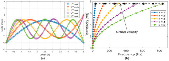
Figure 4.
(a) Normal vibration modes of pipe with no fluid; (b) Impact of modes on critical velocity and frequency in a pipe–fluid system supported be an elastic foundation.
Figure 5 represents the relationship between the dimensionless frequency and dimensionless fluid flow velocity for the first two modes of the pipe. In particular, Figure 5a shows the real part of the first two modes in which the mode has a lower frequency than the second mode after a certain instant is verified a convergence of both modes with a uniform increase in frequency. Figure 5b shows the imaginary part in which the frequency of both modes varnishes until the first mode varies with positive parabolic deviation and then converges and instantaneously diverges symmetrically. The results in Figure 5 closely resemble the findings reported in [30,31] investigated the phenomenon of flow-induced vibration in pipes supported by a two-parameter elastic foundation. Their studies considered a range of boundary conditions, highlighting the dynamic interaction between fluid flow and structural support characteristics.
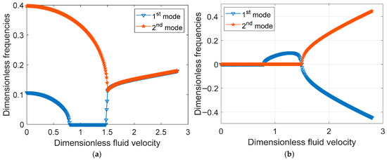
Figure 5.
(a) Real eigenfrequency branches against dimensionless fluid velocity for the two lowest modes; (b) Normalized imaginary eigenfrequency across fluid velocities for the two lowest modes.
4. Physics-Informed Neural Networks for Nonlinear Transverse Vibrations in Free-Tension Pipe Conveying Fluid
Pipes conveying fluid exhibits complex dynamic behaviors, especially under the influence of fluid–structure interactions. When such a pipe is under free-tension, the transverse vibrations become highly nonlinear due to the combined effects of flow velocity, Coriolis forces, inertial coupling, and possible geometric nonlinearities as shown in Equation (8). Traditional numerical methods such as finite difference, finite element, and spectral methods have been extensively used to solve the governing PDE describing these dynamics. However, these methods may suffer from high computational costs, especially for inverse problems, real-time simulations, and parameter identification. PINNs approximate the solution w(x,t) using a deep neural network has a key idea to encode the physics (PDE, boundary, and initial conditions) into the loss function Ψ composed of the following equations.
Figure 6 summarises the end-to-end PINN workflow for the pipe–fluid problem as a compact cycle. The process opens with the governing model: a transverse-vibration PDE for a fluid-conveying pipe on an elastic foundation, including centrifugal and Coriolis effects from axial flow and the foundation reaction term (see Equation (8) and boundary conditions in Equations (9) and (10)). Stochastic forcing is then injected as broadband excitation to reflect laboratory variability and to probe the spectrum under realistic loads. A composite training objective follows, built from three residual families evaluated on the network output interior PDE residuals, boundary-condition residuals, and initial-condition residuals with weights defined in Equations (26)–(30). Collocation points in space–time specify where the physics is enforced. Points concentrate near boundaries and in regions of large gradients, while still covering the full domain for stability over long windows. A simple feed-forward network maps (x,t) to displacement. The architecture is intentionally minimal so that most of the inductive bias comes from the physics terms in the loss rather than from model complexity. Optimization proceeds with RProp, chosen for its step-size adaptation per parameter and reduced sensitivity to heterogeneous residual scales that often appear when PDE, BC, and IC penalties co-exist. Benchmarking closes the learning loop. Predicted fields are compared against analytical modal solutions in frequency domain, checking regression quality and the placement of spectral peaks as flow speed and foundation stiffness vary. Actionable outputs then follow naturally, mode shapes and frequencies, sensitivity trends with respect to parameters, and surrogate responses ready for inverse identification under sparse or noisy conditions. In effect, the wheel encodes a single pass from physics to a trained, differentiable surrogate and back to engineering conclusions, with every slice of the cycle modifying the same object under the composite loss.

Figure 6.
PINN training cycle for pipe–fluid dynamics.
The training of the neural network model was conducted using RProp algorithm in MATLAB R2024b with a configuration details presented in Appendix A. The dataset was randomly divided into training, validation, and testing subsets using the dividerand function to ensure unbiased partitioning. RProp’s with step adaptation parameters reduces sensitivity to the severe loss-scale imbalance and gradient noise typical in PINNs [32,33]. Adam is known to admit non-convergence in simple settings and L-BFGS introduces line-search and memory overhead in full-batch residual evaluations, making RProp a stable, low-overhead choice [34].
Figure 7 shows connected feedforward neural network architecture employed in the PINNs framework, with input layer (x,t), three hidden layers, and a scalar output approximating the solution of the governing PDE. The input layer consists of 2 neurons, corresponding to the spatial coordinate x and temporal coordinate t, which serve as independent variables for the solution . The architecture features three hidden layers, each containing 20 neurons. These neurons are fully connected, meaning every neuron in one layer is connected to every neuron in the subsequent layer. The output layer contains a single neuron, producing the network’s scalar output representing the approximate solution of the PDE at a given spatial-temporal input point.
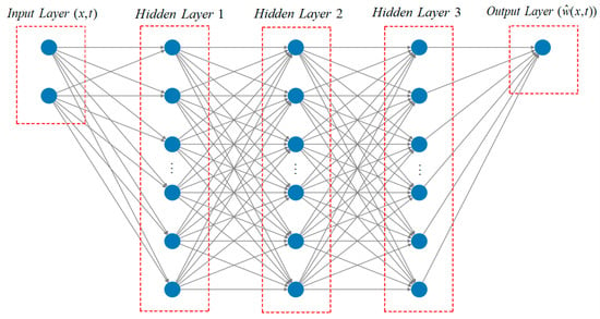
Figure 7.
Neural Network Architecture for the PINNs framework.
Figure 8 illustrates the training configuration and performance diagnostics of PINN developed to approximate the solution of the governing PDE for transverse vibration in a fluid-conveying pipe on an elastic foundation. As shown in Figure 8a, the network architecture comprises an input layer with two neurons representing the spatial and temporal coordinates, followed by three fully connected hidden layers with 20 neurons each, and a single-neuron output layer representing the predicted transverse displacement . The learning process, governed by a loss function embedding the PDE, boundary, and initial conditions, is optimized using RProp algorithm. Figure 8b presents MSE across training, validation, and testing datasets over 319 epochs. The network achieves its best validation performance at epoch 313 with an MSE of 3.484 × 10⁻⁵, indicating rapid convergence and minimal overfitting. Figure 8c further confirms training stability through the consistent decay of the gradient magnitude reaching 0.000486 at epoch 319 and a limited number of validation checks, demonstrating efficient training convergence without early degradation of generalization. Blue circles indicate epochs with zero increment (validation loss improved), while red diamonds indicate epochs with a positive increment, meaning no improvement in validation loss at that check. Finally, Figure 8d displays the error histogram across 20 bins for training, validation, and test sets. The distribution is sharply centred around zero with minimal skewness and narrow spread, confirming that prediction errors are both unbiased and consistently small across all data partitions.
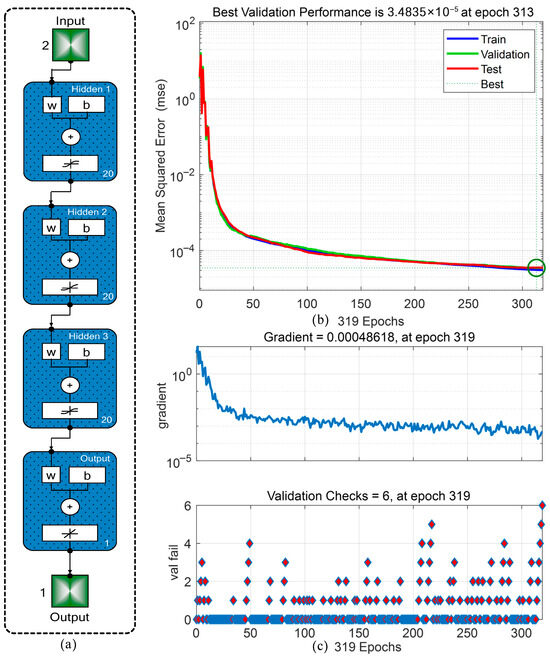
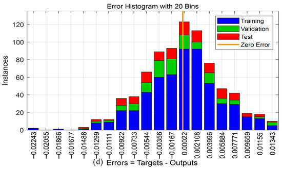
Figure 8.
(a) Feed-forward neural network; (b) Neural network training performance with a green circle marking the epoch where the validation loss attains its minimum; (c) Neural network training state of gradient and validation check; (d) Neural network training error histogram.
Figure 9 presents the regression analysis of PINN model applied to the problem of transverse vibration in a fluid-conveying pipe on an elastic foundation. The four subfigures assess the correlation between the predicted outputs and true target values for the training, validation, testing, and combined datasets. In Figure 9a, the regression coefficient for the training dataset is R = 0.99997, indicating an almost perfect linear fit, with the predicted values closely following the ideal identity line Y = T. Figure 9b displays the regression result for the validation dataset with an R-value of 0.99997, confirming the model’s generalization capability to unseen data. In Figure 9c, the test dataset yields an R-value of 0.99997, further demonstrating that the trained network maintains high predictive accuracy across independent data samples. Lastly, Figure 9d aggregates all data partitions and reports an overall regression coefficient of R = 0.99997, with the fitted regression line nearly overlapping the identity line. The minimal deviations and uniformly high R-values across all subsets confirm the reliability, stability, and predictive consistency of the PINN.
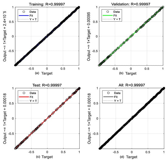
Figure 9.
Neural network training regression: (a) predicted and target values align tightly for the training subset; (b) minimal deviation on the validation subset correlation; (c) predictions align with targets for the held-out test subset; (d) overall correlation remains extremely high across combined datasets.
FFT response of 1st mode of transversal deflection of the pipe conveying fluid shown in Figure 10a demonstrates fluctuation amplitude of vibration. As a result of the phase shift, every other sample element of the FFT output, such as a change in flow speed and excitation frequency from the elastic foundation, is neglected causing the oscillations as observed. Figure 10b shows the reduction in vibration amplitude with two main frequencies higher than the one on 1st mode shown in Figure 10a. In Figure 10c, the FFT is presented with an excited foundation frequency of 15 rad/s corresponding to the 1st natural frequency. The presence of the major component frequency around 3.2 Hz indicates a dominant frequency component in the system. This component likely arises from the dynamic interaction of the pipe and fluid under the influence of the excited foundation. Thus, the main frequency component indicates variation frequencies near 3.2 Hz and stresses this particular frequency as the most influential one for the system response. The 2nd natural frequency is analysed according to the guidelines presented in Figure 10d. Two main frequencies can be underlined, namely 6.4 Hz and 13.7 Hz. These two poles indicate that the signals have distinct frequencies, leading to a more complex oscillation pattern at the second natural frequency. The FFT with an excited foundation frequency ωf = 25 rad/s, presented separately for the 1st and 2nd natural frequencies in Figure 10e,f, respectively. Particularly, at the 1st Natural frequency, the primary oscillation frequency is observed at 2.75 Hz with an amplitude of 0.011 m. On the other hand, at the 2nd Natural frequency, the primary oscillation frequency increases to 6.6 Hz with a reduction in the amplitude of 0.0064 m. The amplitude of the primary oscillation frequency at the 1st natural frequency is 0.011 m, while at the 2nd natural frequency, the amplitude is 0.0064 m. This indicates that the amplitude of the primary oscillation frequency is higher at the 1st natural frequency compared to the 2nd natural frequency. Stability margins are determined by the deterministic eigenvalue and critical velocity condition, while the noise primarily excites near resonant modes and spreads energy across frequency bands observed in the spectra. Practically, the response shows fluctuating amplitudes and mode content at a given flow speed and foundation stiffness, with Coriolis and centrifugal couplings shaping whether the noise driven motion tends toward instability.
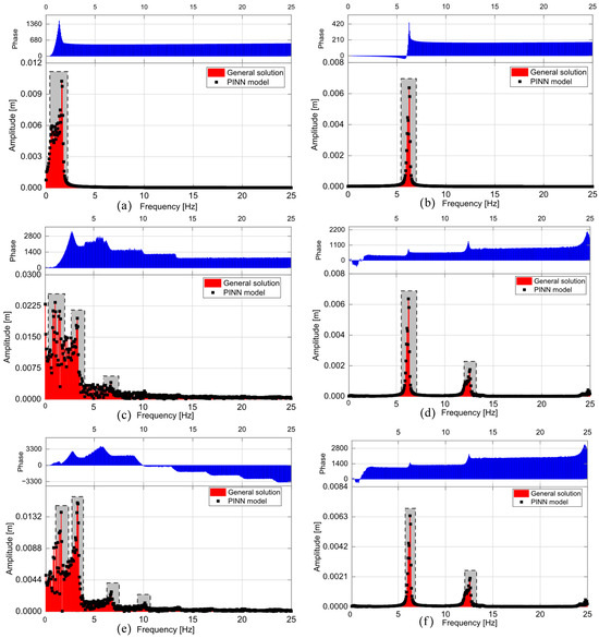
Figure 10.
(a) Mode-1 transverse FFT for ωf = 5 rad/s showing dominant peak and phase, PINN overlay; (b) mode-2 transverse FFT for ωf = 5 rad/s showing dominant peak and phase, PINN overlay; (c) FFT of mode-1 vibration at ωf = 15 rad/s showing dominant lines, PINN comparison; (d) FFT of mode-2 vibration at ωf = 15 rad/s showing dominant lines, PINN comparison; (e) spectral–phase map from FFT, mode 1 at ωf = 25 rad/s, broadband comparison to PINN; (f) spectral–phase map from FFT, mode 2 at ωf = 25 rad/s, broadband comparison to PINN.
5. Conclusions
This study presented preliminary validation hybrid approach for investigating the transverse vibration characteristics of fluid-conveying pipes supported by an elastic Winkler-type foundation under free-tension conditions. The formulation captures complex physical effects, including Coriolis and centrifugal forces, inertial coupling, and stochastic excitation, leading to the derivation of a fourth-order partial differential equation based on Euler–Bernoulli beam theory. Modal analysis was employed to characterize the influence of fluid velocity on the system’s critical buckling behavior. The proposed PINN architecture embeds the governing PDE, initial, and boundary conditions directly into the loss function, enabling accurate and physically consistent approximations of the system’s dynamic response. The network was trained using RProp optimizer and validated through comprehensive statistical metrics, including regression coefficients exceeding R = 0.99997 across all data partitions. Training diagnostics further confirmed convergence stability, minimal overfitting, and uniformly low error distributions. Spectral analysis of the system response further revealed how fluid flow velocity and external excitation frequencies influence the modal behavior and energy distribution across frequency bands. Future work will evaluate noise-robust inverse identification, frequency-rich forcings, and long-duration integration schemes. Future studies should target the specific limitations where PINNs may confer advantages. Priority areas include mitigating spectral bias for high-frequency content via Kernel Density Estimation features and pursuing data-sparse, noise-robust inverse identification with physics-regularised losses as well as comprehensive time-domain accuracy assessments. Additional work should examine stochastic excitations using moment-based PINN variants and address long-duration error control through time-segmented schemes such as AT-PINN.
Author Contributions
Conceptualization and initial development, D.F.S.; methodology, D.F.S., B.X.T. and A.A.A.; software, D.F.S., B.X.T. and A.A.A.; formal analysis of the data, D.F.S.; writing—original draft preparation, D.F.S., B.X.T. and A.A.A.; writing—review and editing, D.F.S., B.X.T. and A.A.A., and all those collaborating in the study. All authors have read and agreed to the published version of the manuscript.
Funding
This research received no external funding.
Institutional Review Board Statement
Not applicable.
Informed Consent Statement
Not applicable.
Data Availability Statement
The original contributions presented in the study are included in the article; further inquiries can be directed to the corresponding author.
Acknowledgments
The authors acknowledge the support from the Department of Industrial Engineering, Operations Management, and Mechanical Engineering, Vaal University of Technology, Vanderbijlpark, South Africa.
Conflicts of Interest
The authors declare no conflicts of interest.
Appendix A. PINN Training Configuration Details
| Item | Value |
| PDE and domain | Fourth-order Euler–Bernoulli-based pipe–fluid PDE with centrifugal and Coriolis terms on a Winkler foundation; free–free BCs; IC as stated in Section 2, Section 3 and Section 4. |
| Inputs and output | Input . Output displacement. |
| Network architecture | Feed forward net ([20], ’trainrp’); hidden activation: tansig; output activation: purelin. MATLAB R2024b. |
| Depth and width | 3 hidden layers, 20 neurons per hidden layer. Rationale aligned with baseline PINNs practice [33]. |
| Loss terms | as in Equations (26)–(30). We used . |
| Collocation points | in the space–time interior; uniform sampling with mild boundary-proximity densification. |
| Supervised data | Targeted points for IC and BC: at for IC; BC points drawn per boundary condition set in Equations (9) and (10). |
| Data split | dividerand random split, default 70% train, 15% validation, 15% test. |
| Optimizer | trainrp (Resilient Backprop). |
| Key training params | epochs = 5000, goal = 1 × 10⁻⁶, validation checks 6 for early stopping, gradient target . Numbers match the training pane and text in Section 4 and Figure 8. |
| Batch size | Full-batch on the assembled residual sets each epoch. |
| Performance metric | Mean squared error mse for reporting. |
| Tooling | MATLAB R2024b Neural Network Toolbox; computations in MEX mode. |
| Diagnostic outcomes | Best validation MSE at epoch 313; gradient reduced to at epoch 319; regression on train, val, test, and all sets; FFT comparisons shown in Figure 10. |
References
- Saari, N.F.; Putra, A.; Irianto; Dan, R.M.; Zeli, M.A.; Ramlan, R.; Jalil, N.A.A.; Herawan, S. Estimating natural frequency of pipe with various geometries: Improvement of frequency factors. Heliyon 2024, 10, e26148. [Google Scholar] [CrossRef]
- Guo, Y.; Ding, H. Theoretical and experimental study on dynamic characteristics of L-shaped fluid-conveying pipes. Appl. Math. Model. 2024, 129, 232–249. [Google Scholar] [CrossRef]
- Duan, J.; Li, C.; Jin, J. Modal analysis of tubing considering the effect of fluid–structure interaction. Energies 2022, 15, 670. [Google Scholar] [CrossRef]
- Weng, G.; Hui, Y.; Cao, J. Time-varying mechanism of fluid-structure interaction vibration effects and dynamic characteristics of the cross-over pipeline when the medium flows. Structures 2023, 57, 105151. [Google Scholar] [CrossRef]
- Zhang, H.; Li, Y.; Xu, Z.; Zhang, A.; Liu, X.; Sun, P.; Sun, X. Modal analysis of PE pipeline under seabed dynamic pressure. Sci. Rep. 2024, 14, 29198. [Google Scholar] [CrossRef]
- Sozinando, D.F.; Tchomeni, B.X.; Alugongo, A.A. Modal analysis and flow through sectionalized pipeline gate valve using FEA and CFD technique. J. Eng. 2023, 2023, 2215509. [Google Scholar] [CrossRef]
- Sozinando, D.F.; Tchomeni, B.X.; Alugongo, A.A. Experimental study of coupled torsional and lateral vibration of vertical rotor-to-stator contact in an inviscid fluid. Math. Comput. Appl. 2023, 28, 44. [Google Scholar] [CrossRef]
- Kanwal, G.; Ahmed, N.; Nawaz, R. A comparative analysis of the vibrational behavior of various beam models with different foundation designs. Heliyon 2024, 10, e26491. [Google Scholar] [CrossRef]
- Xu, L.; Ma, M. Vibration characteristic analysis of tunnel structure buried in elastic foundation based on dynamic stiffness matrix. Int. J. Struct. Stab. Dyn. 2022, 22, 2250173. [Google Scholar] [CrossRef]
- Kanwal, G.; Nawaz, R.; Ahmed, N. Analyzing the effect of rotary inertia and elastic constraints on a beam supported by a wrinkle elastic foundation: A numerical investigation. Buildings 2023, 13, 1457. [Google Scholar] [CrossRef]
- Xiang, Q.; Zeng, R.; Ma, Y.; Ruan, R.; Shen, Y.; Li, S.; Feng, A.; You, Y. Stability and vibration analysis of a fluid-conveying pipe on a two-parameter foundation under general boundary conditions. Phys. Fluids 2025, 37, 014130. [Google Scholar] [CrossRef]
- Li, Z.-M.; Liu, T. A new displacement model for nonlinear vibration analysis of fluid-conveying anisotropic laminated tubular beams resting on elastic foundation. Eur. J. Mech.-A/Solids 2021, 86, 104172. [Google Scholar] [CrossRef]
- Zhou, J.; Chang, X.; Xiong, Z.; Li, Y. Stability and nonlinear vibration analysis of fluid-conveying composite pipes with elastic boundary conditions. Thin-Walled Struct. 2022, 179, 109597. [Google Scholar] [CrossRef]
- Zhang, T.; Yan, R.; Zhang, S.; Yang, D.; Chen, A. Application of Fourier feature physics-information neural network in model of pipeline conveying fluid. Thin-Walled Struct. 2024, 198, 111693. [Google Scholar] [CrossRef]
- Yin, G.; Janocha, M.J.; Ong, M.C. Physics-Informed Neural Networks for Flow-Induced Vibration Prediction of a Subsea Pipeline. In Proceedings of the ASME 2024 43rd International Conference on Ocean, Offshore and Arctic Engineering, Singapore, 9–14 June 2024; American Society of Mechanical Engineers: New York, NY, USA, 2024; Volume 87837, p. V05BT06A080. [Google Scholar]
- Chen, Z.; Lai, S.-K.; Yang, Z. AT-PINN: Advanced time-marching physics-informed neural network for structural vibration analysis. Thin-Walled Struct. 2024, 196, 111423. [Google Scholar] [CrossRef]
- Chai, X.; Cao, W.; Li, J.; Long, H.; Sun, X. Overcoming the spectral bias problem of physics-informed neural networks in solving the frequency-domain acoustic wave equation. IEEE Trans. Geosci. Remote Sens. 2024, 62, 5923520. [Google Scholar] [CrossRef]
- Lee, J.; Park, K.; Jung, W. Physics-Informed Neural Networks for Cantilever Dynamics and Fluid-Induced Excitation. Appl. Sci. 2024, 14, 7002. [Google Scholar] [CrossRef]
- Liu, Y.; Hou, J.; Wei, P.; Jin, J.; Zhang, R. Research and application of ROM based on Res-PINNs neural network in fluid system. Symmetry 2025, 17, 163. [Google Scholar] [CrossRef]
- Zhu, P.; Liu, Z.; Xu, Z.; Lv, J. An Adaptive Weight Physics-Informed Neural Network for Vortex-Induced Vibration Problems. Buildings 2025, 15, 1533. [Google Scholar] [CrossRef]
- Zhou, W.; Miwa, S.; Okamoto, K. Advancing fluid dynamics simulations: A comprehensive approach to optimizing physics-informed neural networks. Phys. Fluids 2024, 36, 013615. [Google Scholar] [CrossRef]
- Ang, E.H.W.; Wang, G.; Ng, B.F. Physics-informed neural networks for low Reynolds number flows over cylinder. Energies 2023, 16, 4558. [Google Scholar] [CrossRef]
- Kim, G.-Y.; Lim, C.; Kim, E.S.; Shin, S.-C. Prediction of dynamic responses of flow-induced vibration using deep learning. Appl. Sci. 2021, 11, 7163. [Google Scholar] [CrossRef]
- Zhao, P.; Xu, Z.; Liu, H.; Yu, B. Unraveling air–water two-phase flow patterns in water pipelines based on multiple signals and convolutional neural networks. Aqua-Water Infrastruct. Ecosyst. Soc. 2023, 72, 2472–2486. [Google Scholar] [CrossRef]
- Chen, H.; Dang, Z.; Hugo, R.; Park, S. CNN-based flow pattern identification based on flow-induced vibration characteristics for multiphase flow pipelines. In Proceedings of the 2022 14th International Pipeline Conference, Calgary, AB, Canada, 26–30 September 2022; American Society of Mechanical Engineers: New York, NY, USA, 2022; Volume 86588, p. V003T04A003. [Google Scholar]
- Wang, X.Q.; Xie, W.-C.; So, R.M.C. Force Evolution Model for Vortex-Induced Vibration of an Elastic Cylinder in a Cross Flow. In Proceedings of the ASME 2006 Pressure Vessels and Piping/ICPVT-11 Conference, Vancouver, BC, Canada, 23–27 July 2006; Volume 47888, pp. 513–520. [Google Scholar]
- Cheng, C.; Meng, H.; Li, Y.-Z.; Zhang, G.-T. Deep learning based on PINN for solving 2 DOF vortex induced vibration of cylinder. Ocean Eng. 2021, 240, 109932. [Google Scholar] [CrossRef]
- Fu, D.; Deng, B.; Yang, M.; Zhen, B. Analytical solution of overlying pipe deformation caused by tunnel excavation based on Pasternak foundation model. Sci. Rep. 2023, 13, 921. [Google Scholar] [CrossRef] [PubMed]
- Khot, S.M.; Khaire, P.; Naik, A.S. Experimental and simulation study of flow induced vibration through straight pipes. In Proceedings of the 2017 International Conference on Nascent Technologies in Engineering (ICNTE), Vashi, India, 27–28 January 2017; IEEE: New York, NY, USA, 2017; pp. 1–6. [Google Scholar]
- Ma, Y.; You, Y.; Chen, K.; Feng, A. Analysis of vibration stability of fluid conveying pipe on the two-parameter foundation with elastic support boundary conditions. J. Ocean Eng. Sci. 2024, 9, 616–629. [Google Scholar] [CrossRef]
- Balkaya, M.; Kaya, M.O. Analysis of the instability of pipes conveying fluid resting on two-parameter elastic soil under different boundary conditions. Ocean Eng. 2021, 241, 110003. [Google Scholar] [CrossRef]
- Igel, C.; Hüsken, M. Empirical evaluation of the improved Rprop learning algorithms. Neurocomputing 2003, 50, 105–123. [Google Scholar] [CrossRef]
- Raissi, M.; Perdikaris, P.; Karniadakis, G.E. Physics-informed neural networks: A deep learning framework for solving forward and inverse problems involving nonlinear partial differential equations. J. Comput. Phys. 2019, 378, 686–707. [Google Scholar] [CrossRef]
- Wang, S.; Yu, X.; Perdikaris, P. When and why PINNs fail to train: A neural tangent kernel perspective. J. Comput. Phys. 2022, 449, 110768. [Google Scholar] [CrossRef]
Disclaimer/Publisher’s Note: The statements, opinions and data contained in all publications are solely those of the individual author(s) and contributor(s) and not of MDPI and/or the editor(s). MDPI and/or the editor(s) disclaim responsibility for any injury to people or property resulting from any ideas, methods, instructions or products referred to in the content. |
© 2025 by the authors. Licensee MDPI, Basel, Switzerland. This article is an open access article distributed under the terms and conditions of the Creative Commons Attribution (CC BY) license (https://creativecommons.org/licenses/by/4.0/).