Ensemble-Based Refinement of Landmark Annotations for DNA Ploidy Analysis in Digital Pathology

Featured Application

Constructing an ensemble from assay-specific segmentation algorithms can improve the available ground truth dataset. A refined ground truth can support more reliable evaluation and validation of image analysis algorithms. For niche assay topics, where annotated data is limited and expensive to produce, this approach provides a way to generate or improve annotations without extensive manual work. In practice, this can help laboratories working with DNA ploidy and similar tasks to strengthen their datasets, reduce annotation bias, and improve algorithm development specific to their field.

Abstract

Reliable evaluation of image segmentation algorithms in digital pathology depends on high-quality annotation datasets. Landmark-type annotations, essential for cell-counting analyses, are often limited in quality or quantity for segmentation benchmarking, particularly in rare assays where annotation is scarce and costly. In this study, we investigate whether ensemble-inspired refinement of landmark annotations can improve the robustness of segmentation evaluation. Using 15 fluorescently imaged blood samples with more than 20,000 manually placed annotations, we compared three segmentation algorithms—a threshold-based method with clump splitting, a difference-of-Gaussians (DoG) approach, and a convolutional neural network (StarDist)—and used their combined outputs to generate an ensemble-derived ground truth. Confusion matrices and standard metrics (F1 score, precision, and sensitivity) were computed against both manual and ensemble-derived ground truths. Statistical comparisons showed that ensemble-refined annotations reduced noise and decreased mean offsets between annotations and detected objects, yielding more stable evaluation metrics. Our results demonstrate that ensemble-based ground truth generation can guide targeted revision of manual markers, provide a quality measure for annotation reliability, and generate new annotations where no human-generated landmarks exist. This methodology offers a generalizable strategy to strengthen annotation datasets in image cytometry, enabling robust algorithm evaluation in DNA ploidy analysis and potentially in other low-frequency assays.

1. Introduction

DNA ploidy analysis, a laboratory technique assessing DNA content in a cell′s nucleus, classifies cells by their ploidy status—indicating complete chromosome sets. Crucial in cancer research, it identifies abnormal DNA content, aiding diagnosis and treatment decisions. To quantify DNA content, staining with a dye proportional to DNA content is essential. These samples can be digitized through fluorescent imaging, where the dye, when excited by specific wavelength light, emits light of a different wavelength. In this study, propidium iodide staining was employed. This emitted light is the basis of the measurement. In this project the sample used is nuclei from blood, but any other body tissues can be used, as long as they contain DNA. The traditional appliance for this task is a flow cytometer, and the technique, in broader terms, is called flow cytometry (FCM). The working principle is simple: a light source (usually a laser) and a detector, with objects to measure passing in a capillary tube between the two. The “shadow” the passing objects cast on the detector generate the data for the classification [1]. Of course, modern flow cytometers contain multiple light sources of different wavelengths and multiple detectors. This technology is widely used today, and is still being continuously developed, and has its pros and cons [2].

In our project we aim to utilize digital slide scanners and image analysis to achieve the same goal. In laboratories, where such devices are available, they offer several advantages, including the ability to store samples in digital form for an indefinite period. Formalin-fixed paraffin-embedded sample blocks need to be preserved for many years—often decades—according to medical regulations worldwide. In the case of fluid samples, this was not viable. The increasing importance of quality control in medical laboratories alone can drive technological transition. Processing of the sample for analysis is identical up to the step of placing it into the flow cytometer. Digital slide scanners ingest glass microscopy slides, so the sample is placed on one as a droplet and covered with a glass coverslip to be digitized. This approach of analyzing cell populations via image processing is called image cytometry (ICM).

Our broader project is to explore the possibilities of this approach for DNA ploidy using ICM. The proof of concept was established and published earlier within the topics of object segmentation [3,4] and population analysis [5,6]. Figure 1 shows the schematic representation of the project.

Refining the proof of concept in place was our next goal. The recent advances in image processing, especially deep learning-based processing, offered an opportunity to enhance the object segmentation portion of the workflow.

In digital image cytometry, a recurring limitation is the availability and consistency of annotated data needed for training and evaluation, rather than the algorithms themselves.

Fluorescent images are scarce; ones for ploidy analysis are even more so. Creating an annotated dataset in this topic is a considerable effort. Similar problems have been reported [7]. Here, we took a different approach by reusing a dataset originally annotated for segmentation development. We decided to use that dataset for evaluation of other options available first. Evaluation of image processing solutions is a common topic; there is an example even in the field of fluorescent imaging [8].

Our prior analysis covered algorithms of three complexity levels. The first, labeled Algorithm 1, is a straightforward threshold-based approach enhanced by the clump splitting algorithm we developed [3,4]. We introduced an additional step to improve the detection of low-intensity objects in the image not dissimilar to the one described in [9]. The second, named Algorithm 2, is a more intricate classical algorithm based on the difference of Gaussians [10]. The third, Algorithm 3, is a modern CNN-based approach [11].

These algorithms were selected primarily to probe the complexity of the segmentation task, but these three algorithms also represent distinct inductive biases—threshold-based morphology, gradient space filtering, and learned shape priors—providing complementary error patterns for ensemble refinement.

Table 1. Overview of the three segmentation algorithms used in this study, including their core principles, key characteristics, and approximate computational complexity.

Algorithm	Core Principle	Key Characteristics	Relative Computational Complexity
Algorithm 1	Threshold-based segmentation with clump-splitting and low-intensity enhancement	Adaptive threshold level; morphological separation factor	Adaptive threshold level; morphological separation factor
Algorithm 2	Difference-of-Gaussians (classical gradient filtering)	Gaussian smoothing with multi-scale contrast enhancement; blob detection via local intensity differences.	Moderate—convolutional filtering, pixel-wise gradient analysis
Algorithm 3	CNN-based (StarDist) with star-convex polygon representation	Network depth and receptive field; number of star rays	High—deep network inference, nonlinear computational cost

summarizes their core principles, key characteristics, and relative computational complexity. Figure 2 contains a sample of the segmentation results of the three algorithms.

For evaluating these image segmentation algorithms, we utilized the manually placed landmark-type annotations that were originally generated for the development of our own algorithm. Annotation of medical images is a complex topic [12]. In particular, the task of segmenting cells on fluorescent images on our dataset is challenging due to the simplicity of the available annotation data. For the development of Algorithm 1, more than 20,000 objects were annotated with single-point markers—an approach usually referred to as landmark annotation. This dataset was subsequently used to evaluate and compare the selected algorithms.

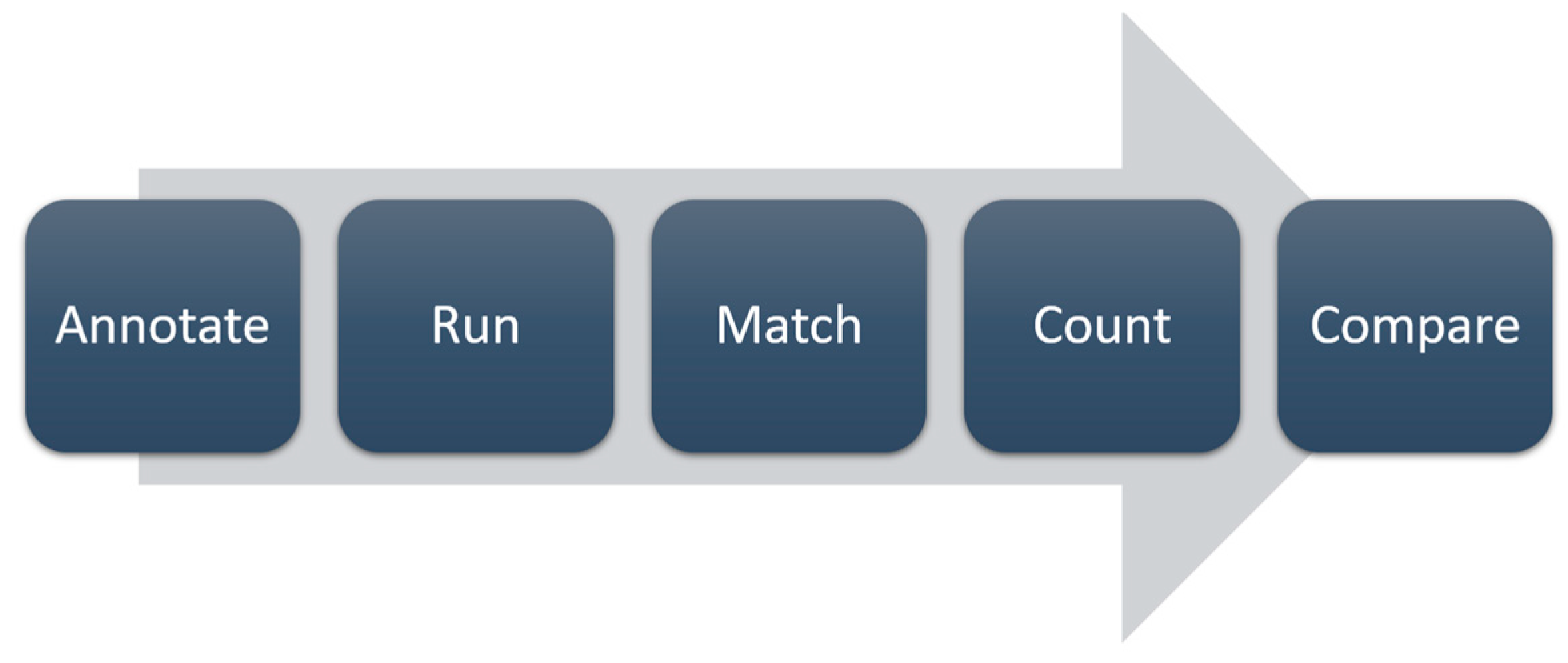
We chose to use a confusion matrix-based approach [13] to compare our candidates through F1 score, precision, and sensitivity, as has also been carried out in [14]. The main steps of this process are illustrated in Figure 3.

The results showed partial inconsistency between the visual and quantitative evaluations. While the two more advanced algorithms yielded visually superior segmentations, their measured improvements were smaller than anticipated. Further inspection revealed that this ground truth dataset is sub-optimal for this task; it has undesirable characteristics that decrease the accuracy of the comparison, and which we aimed to mitigate.

The first goal of this investigation is to find an evaluation framework that is better suited for algorithm comparison. This fundamentally means we are looking to enhance our manually created ground truth, which is challenging, because it served as the frame of reference in our previous analyses.

To achieve this goal, we utilized the three algorithms described above, each achieving an F1 score above 0.7 on our samples and therefore providing a representative coverage of the segmentation problem. When considered as an ensemble, they represent a set of distinct algorithmic perspectives on the task of detecting and segmenting the cell nuclei in the samples. Unifying their results and contrasting them against the original ground truth can aid in highlighting those annotations that we should consider revising. The combined result of the ensemble can be used to replace the manually produced markers, where deemed necessary. In some cases, it may even generate a high-quality ground truth, even where there is no manual annotation present.

The inspiration came from ensemble classifiers, like random forest [15] or xgboost [16], but large language models have also been merged into ensembles recently in order to achieve even better performance [17].

We hypothesize that integrating outputs of complementary segmentation algorithms can refine landmark annotations and improve the stability of algorithm evaluation metrics.

2. Materials and Methods

2.1. Samples

For this evaluation we used 15 samples of leftover healthy human blood samples containing only propidium iodide-stained cell nuclei. The samples were placed on a glass slide after serving their original purpose in a flow cytometer. They were coverslipped and digitized using a glass slide scanner produced by 3DHISTECH Ltd., Budapest, Hungary (Pannoramic Scan, fluorescent setup, 5 MP sCMOS camera, 40× (Carl Zeiss AG, Jena, Germany) objective lens and an LED-based light source). The resulting resolution of the images were 0.1625 µm/pixel (compressed with jpeg, to quality 80). The ICM measurements were taken on sub-samples of these samples, sampled as lab protocols demand, in the amount to fit on a covered glass slide. The samples were identified by their sequential indices throughout the assay (1M01-1M20). The samples contain a droplet approximately 15 mm in diameter. This means approximately a 180 mm² area populated with nuclei; roughly 7 gigapixels to process. The algorithms’ input was an 8-bit, single-channel image that was ingested by the algorithms in a tiled manner. (Sample numbering also contains images not participating in the study due to preparation failure and the bleaching effect of fluorescent samples. Setting up the digitization process and parameters wears out the dye, and that changes the intensity of the images used).

All samples used in this study were anonymized and originated from previously published, ethically approved work [7]. No new human or animal experiments were conducted.

2.2. Annotation

Rectangular regions of 1 mm² were selected on each sample for validation, containing from ~830 to ~2200 annotated nuclei. An expert with laboratory experience was cooperating in placing the annotations.

Visible artifacts like bubbles, clumping, and unwashed/overexposed staining were avoided when selecting the regions to evaluate. Ground truth: The cells visible on the digital samples were annotated using the Pannoramic Viewer 1.15.3 (3DHISTECH Ltd., Budapest, Hungary) software’s Marker Counter tool. The resulting annotation is a simple coordinate pair, defined on the plane coordinate system of the digital slide.

2.3. Segmentation Algorithms

We utilized three segmentation algorithms: a threshold-based method with clump splitting (Algorithm 1), a difference-of-Gaussians approach (Algorithm 2), and a convolutional neural network (StarDist, Algorithm 3). Detailed descriptions of the algorithms and parameter settings have previously been reported in [18]. In this work, we summarize their essential principles for clarity, while referring the reader to the earlier publication for complete implementation details. The specific algorithms are of lesser importance in this study; what matters is their ability to achieve high accuracy, thus providing a good representation of the object detection task on these samples.

2.4. Running the Segmentation Algorithms

The algorithms evaluated were implemented as a plugin for QuantCenter RX 2.4, the image processing software suite of 3DHISTECH Ltd. Algorithm 3 used the python library StarDist [11]. The evaluation framework was also implemented in Python language.

Both the segmentation algorithms and the validation were run on a mobile PC with an Intel(R) Core(TM) i5-9400H CPU, 32 GB of RAM, with Python 3.11 on Windows 10 Pro 22H2.

2.5. Evaluation Configurations, Comparison, Generation

The initial task is to compare polygonal segmentation objects produced by an algorithm to landmark-type annotations. An assignment must be made between the annotations and measurement results to form matched pairs [19], in the following form:

$$f\left(A_i{,O}_j\right)=\left\{\begin{array}{c}1, | A_i is assigned to O_i\\ 0, otherwise\end{array}\right.$$

(1)

where Ai and Oi are the annotation and object, respectively.

For matching, we chose two approaches: a greedy (best-first) and a linear optimization [20].

To be able to compare multiple options in object representation and assignment algorithms, a new metric must be introduced, instead of the current ground truth.

The natural choice is the sum of distances of all the assigned pairs. A cost matrix is needed, again with the annotations and the objects on the row and column headers, and the Euclidean distance between them. It can be written as

$$C\left(A_i{,O}_j\right)=d_E\left(a_i{,o}_j\right)$$

(2)

where ai and oi are single-point representations of annotation and object, respectively, and

$$d_E\left(a_i{,o}_j\right)=\sqrt[2]{{\left(a_{ix}-o_{jx}\right)}^2+{\left(a_{iy}-o_{jy}\right)}^2}$$

(3)

For computational complexity reduction the squared distance was used

$${d_E\left(a_i{,o}_j\right)}^2={\left(a_{ix}-o_{jx}\right)}^2+{\left(a_{iy}-o_{jy}\right)}^2=c\left(a_i{,o}_j\right)$$

(4)

We also introduced a distance limit that prevents assignments that are not valuable from the task perspective.

$$f^{’}\left(A_i{,O}_j\right)=\left\{\begin{array}{c}1, | A_i is assigned to O_i, and {d_E\left(a_i{,o}_j\right)}^2<{maxThreshold}^2\\ 0, otherwise\end{array}\right.,$$

(5)

where maxThreshold is a constant set to 30 pixels. This value corresponds to approximately half the average nuclear radius in our dataset (≈4.9 µm), ensuring that assignments remain biologically meaningful while tolerating minor annotation imprecision. The approximation was derived from the mean segmented object area across all samples.

To be able to compare the different configurations, we used the sum of the costs of the matches for each sample in S as follows:

$$c_S= \sum _{\mathrm{0,0}}^{i,j}\left(c\left(a_i{,o}_j\right)f’\left(A_i{,O}_j\right)\right)$$

(6)

We used the means to represent each configuration with a single value.

$$c_T=\sum _0^s\left(c_S\right)/n\left(S\right)$$

(7)

This model is controversial in some respects: the cost of the assignments thus filtered were not included in the evaluation. This covered two error classes: valid matches, which were too far from each other, and invalid matches. The direct inclusion of the distances themselves seemed an inadequate choice, because they often were magnitudes larger than the mean/median of the distances of the successfully matched pairs (thus overshadowing the important values of the valid matches). To counterweigh that effect, we chose to use a penalty value for these filtered assignments equal to the threshold value. This penalty value was used also for all unmatched markers uniformly, thus clamping the penalty on a non-accepted match. The penalty term acts as a robust loss component, limiting the influence of outlier matches, consistent with the principles of robust statistics. The three parameters described above were summed as total assignment cost and were used to rank the configurations.

We used two types of single-point representations for each polygonal object: one based on its centroid, and another based on the centroid of its bounding box (or minimal bounding rectangle). In both cases we consider the centroid to be the arithmetic mean position of all the points in the surface of the figure.

Another approach can be to maintain the polygonal object representation and use the inclusion of the annotation as the assignment algorithm. Here again a greedy approach was chosen, the first inclusion was used, eliminating both annotation and object from the matching process.

Five different configurations were formed based on which we evaluated our algorithms; these are summarized in

Table 2. Evaluation configurations examined.

Pairing Method	Object Representation
Greedy	polygon centroid
	bounding box centroid
Optimized	polygon centroid
	bounding box centroid
Point in polygon

.

Two cost matrices were calculated for comparability: one for bounding box center representations, the other for all the polygonal representations. The method with the value highlighted was chosen to proceed.

The three selected algorithms can be utilized as an ensemble-inspired setup to form an evaluation framework for the ground truth itself. We chose the configuration with the lowest total cost and used its results to construct the new ground truth.

For each annotation a set of points were matched; potentially one from each algorithm. The original annotation was replaced by the centroid of the centroids of the matched objects. The possible cases are generated by the number of such matched objects (zero to three).

We re-evaluated our 3 algorithms (and additionally the original ground truth) to this new ground truth and plotted the two-dimensional offset histograms to have a visual representation about the relation between them.

3. Results

3.1. Cost Comparison

The described cost function produced the summed Euclidean distances for each configuration; these results are summarized in

Table 3. Comparison of assignment methods based on the total cost, over the samples. The values are Euclidean distance squares, summed over the assigned annotation-object pairs.

Pairing Method	Object	Algorithm			Mean	SD
		1	2	3
Greedy	polygon centroid	2.00 × 108	1.72 × 108	1.71 × 108	1.81 × 108	1.34 × 107
	bounding box centroid	2.00 × 108	1.72 × 108	1.71 × 108	1.81 × 108	1.34 × 107
Optimized	polygon centroid	1.79 × 105	2.24 × 105	2.23 × 105	2.09 × 105	2.12 × 104
	bounding box centroid	1.84 × 105	2.27 × 105	2.26 × 105	2.12 × 105	2.01 × 104
Point in polygon		7.51 × 107	1.91 × 105	2.74 × 105	2.52 × 107	3.53 × 107

. The optimized assignment kept its advantage after constraining the assignment and adding penalty values for non-assigned markers. The two object representations performed very similarly (though in the non-penalized model the bounding box centers performed slightly worse with respect to the mean, and better in standard deviation).

3.2. Comparison to the Generated Marker

Across the three algorithms, ensemble refinement improved F1-scores substantially compared to manual GT. The threshold-based algorithm increased from 0.8072 to 0.9755 (+20.85%), the DoG method from 0.8490 to 0.9501 (+11.91%), and the CNN (StarDist) from 0.8461 to 0.9366 (+10.70%). Evaluating precision and sensitivity separately can provide more insight. The corresponding results are summarized in

Table 4. Comparison of segmentation performance metrics (F1-score, precision, and sensitivity) for the three algorithms and the original ground truth after ensemble-based refinement.

	F1 Score	Precision	Sensitivity
Algorithm 1	0.9755	0.9538	0.9986
Algorithm 2	0.9501	0.9064	0.9991
Algorithm 3	0.9366	0.8817	0.9994
Original GT	0.9600	0.9248	0.9983

.

It is important to note that the segmentation algorithms were not re-run; only their existing outputs were re-evaluated against the refined ground truth. These consistent gains demonstrate that ensemble GT reduces annotation noise and yields more stable evaluation metrics.

3.3. Offset Maps

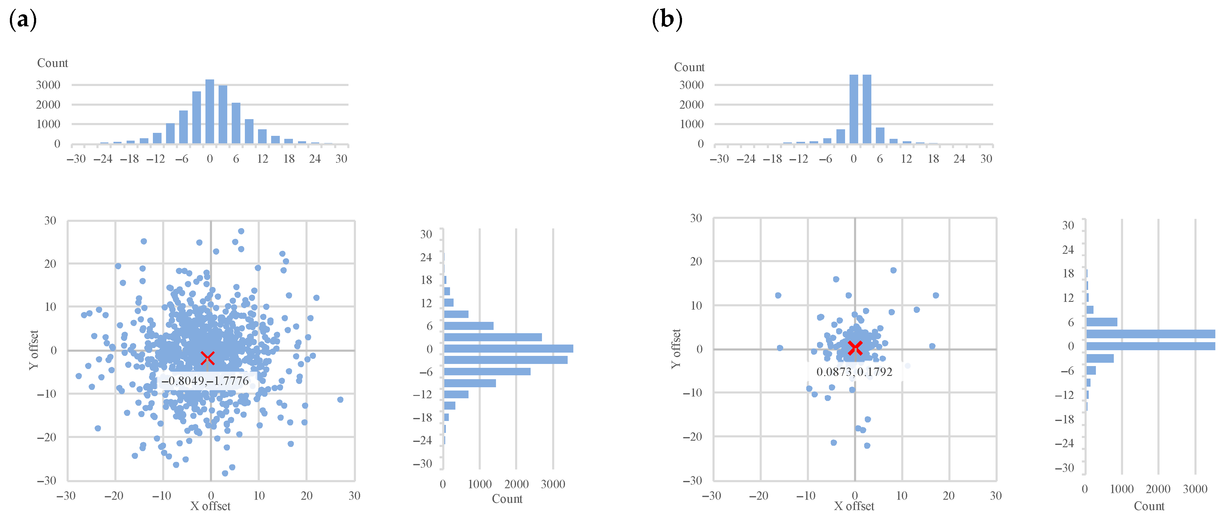
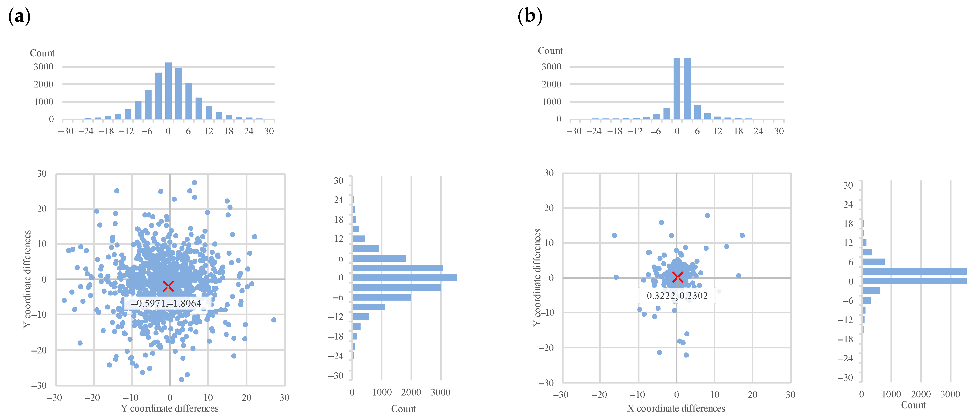
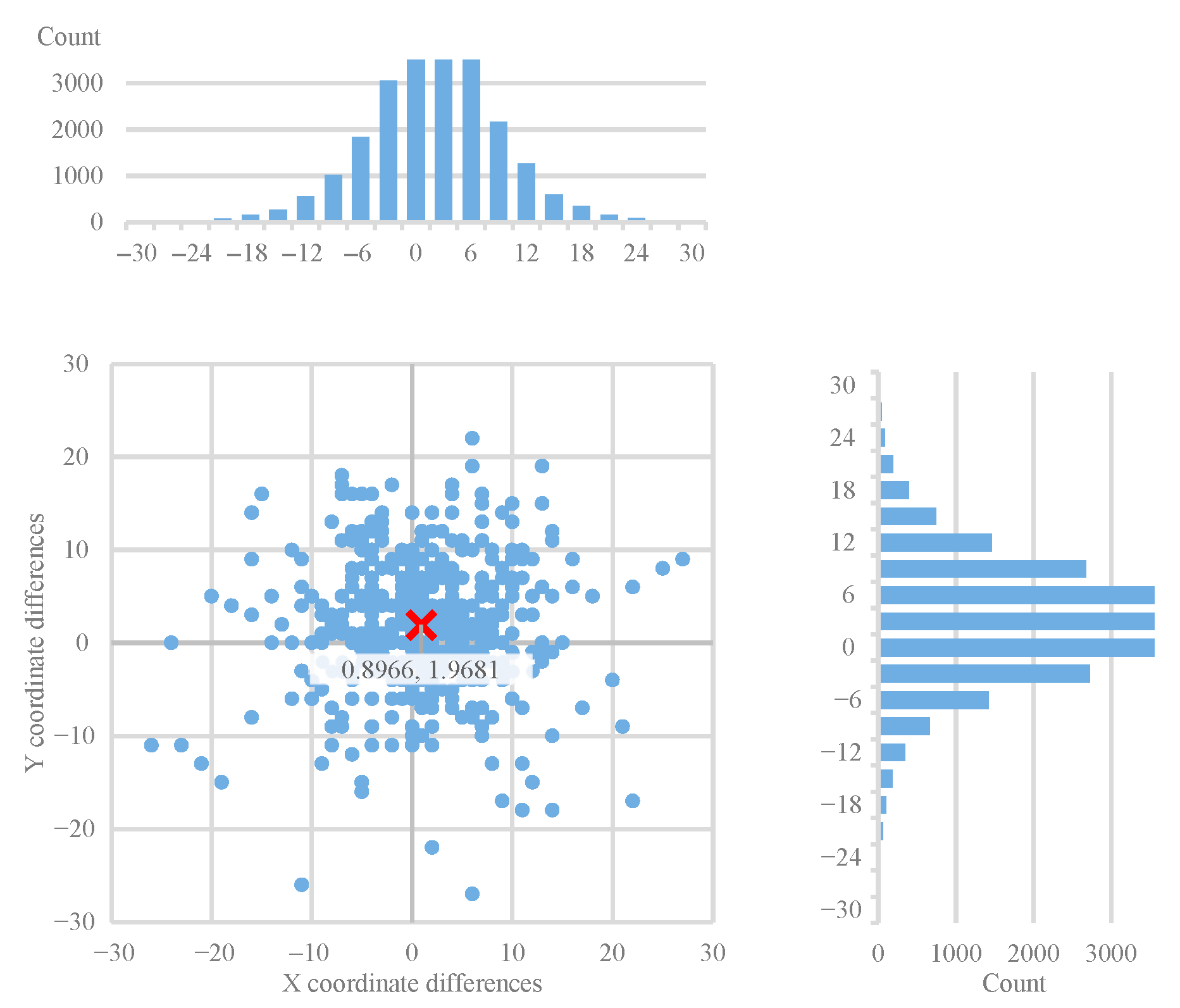
Figure 4, Figure 5 and Figure 6 show the differences between the manually created and the generated offsets mapped on the two-dimensional plane, each chart containing 500 randomly sampled items from the original dataset. The charts are paired—algorithmic results to the manual ground truth dataset are on the left, and the results of the same algorithm against the new ensemble-generated ground truth on the right. They visualize the results for Algorithm 1, 2, and 3, respectively.

Figure 7 is a retrospective checkl we validated the manual ground truth dataset against the new ensemble-generated one, as if it were another segmentation algorithm.

Both the manually placed and the generated markers represent pixel-locations on the digital slide, meaning that both datasets contain integer-valued pixel coordinates. This explains the quantized nature of the last scatterplot, in contrast to the others above.

3.4. Offset Map Summary

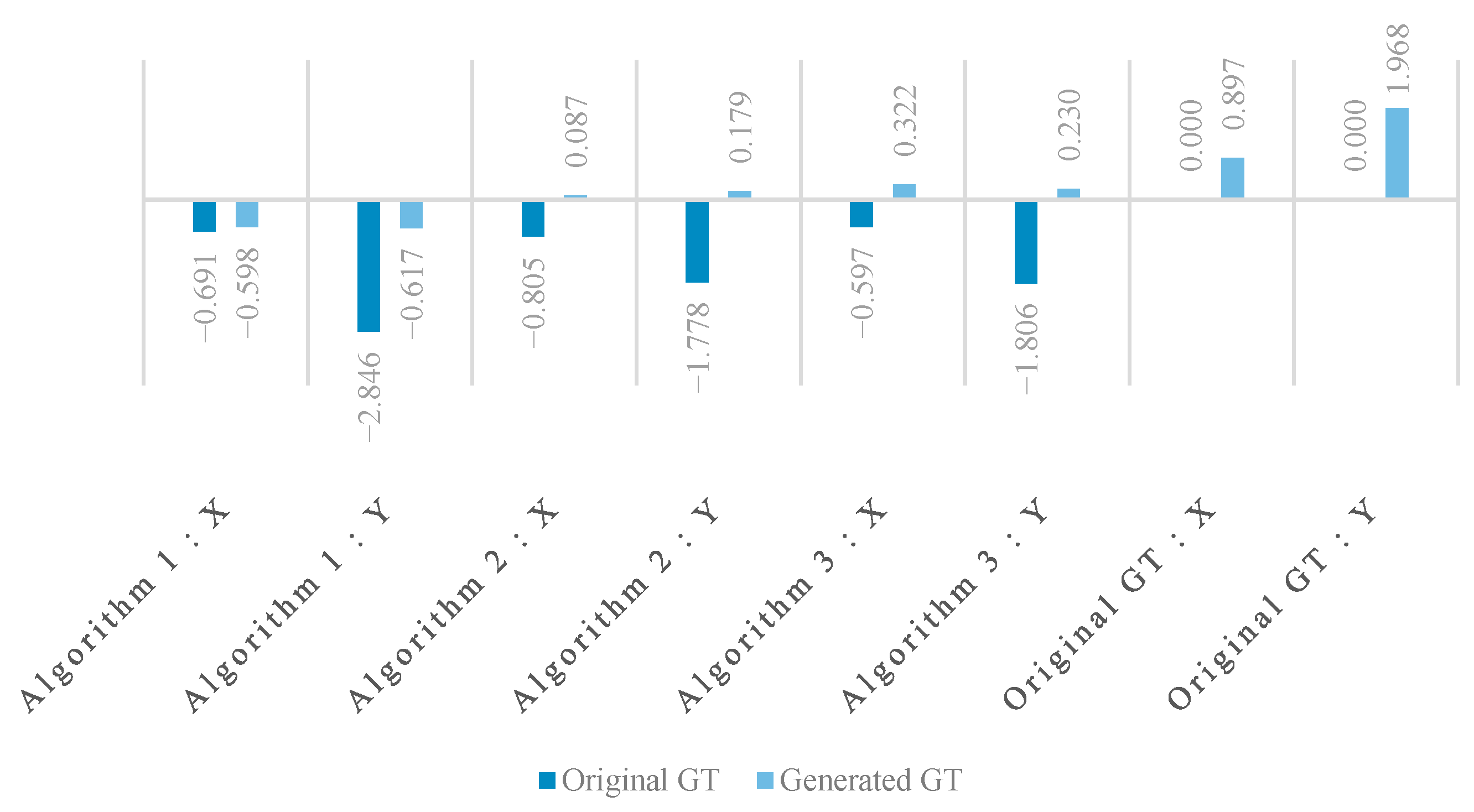
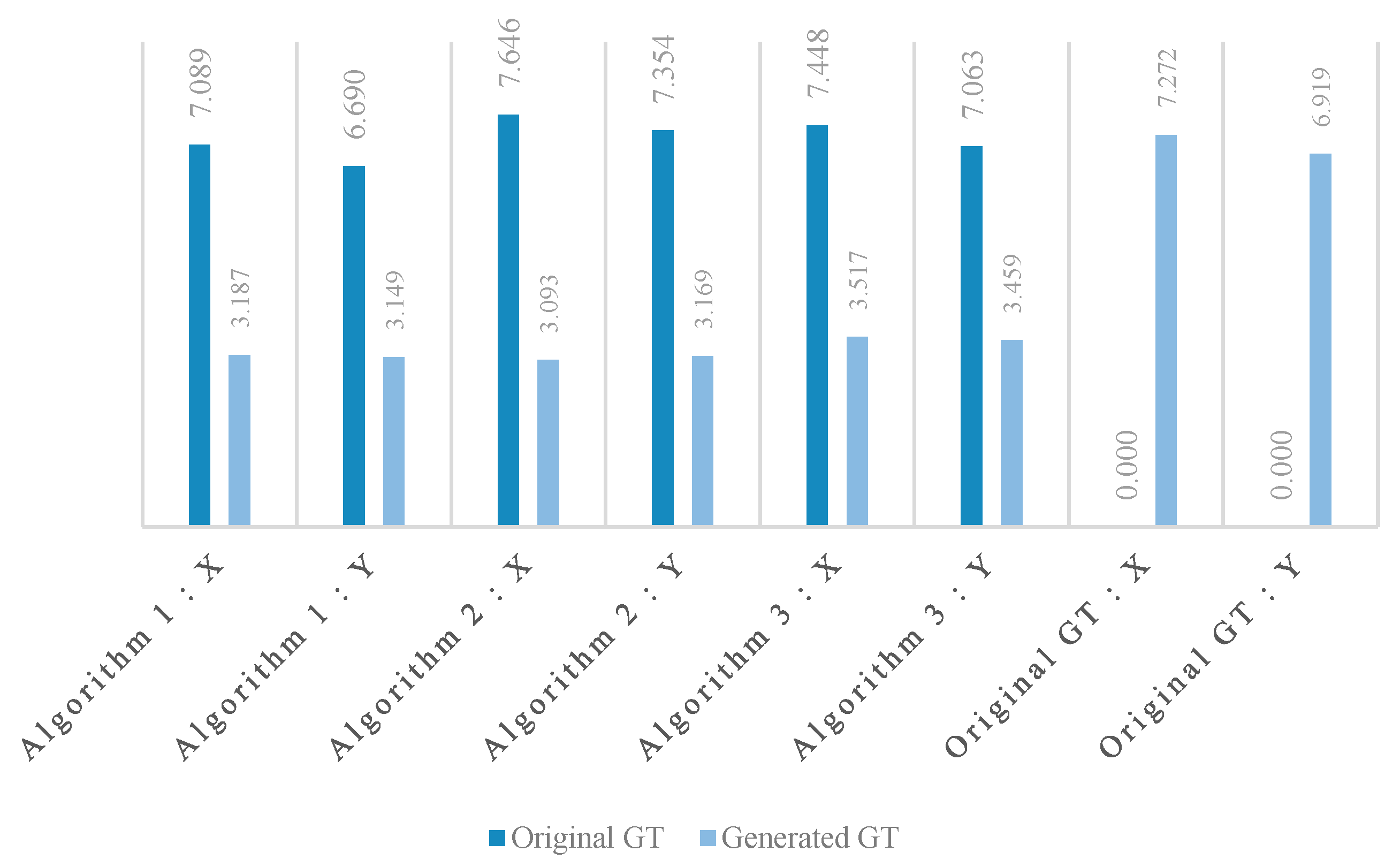
Figure 8 and Figure 9 summarize the offset distributions. Figure 8 shows the mean offsets in X and Y directions, while Figure 9 presents the corresponding standard deviations. Together, they provide a more compact and interpretable view of the improvements achieved.

4. Discussion

Regarding the evaluation framework, based on the measured sum error we chose the configuration with the lowest total error or offset distance. Based on the calculated error visible in Table 2, we used the results of the optimized polygon centroids method to construct the new ground truth. The refined ground truth reduces the risk of overfitting to noisy ground truth thus making the validation of algorithms more trustworthy.

As reported in our earlier study [18], Algorithms 1, 2, and 3 achieved F1-scores of 0.8072, 0.849, and 0.8461, respectively (referring to the macro-averaged data, containing the lower values). For the new ground truth, these values increased to 0.9755, 0.9501, and 0.9366 (Table 3). The improvement was expected because these algorithms participated in the generation of the new ground truth; however, the consistent improvements across all algorithms—ranging from +10.7% to +20.9% in F1-score—highlight the general utility of ensemble refinement. Importantly, this trend suggests that the method strengthens evaluation.

The F1-score of the old ground truth dataset against the new generated one is also telling; it retained a 0.9600 F1-score, and that means that it represents the original dataset well.

We included all the offset maps, showing the differences between the ground truth landmarks (both original and generated) and the objects detected by the three algorithms. These show the differences in two dimensions, and we added projected histograms to show the distribution of these data points. Here the important results are the decrease in the offsets (Figure 8) and their standard deviations (Figure 9) in both X and Y directions between the ground truth landmarks and the objects detected by all three algorithms.

It is interesting to note that in Figure 8 the horizontal and vertical offsets differ considerably when using the ensemble-generated new ground truth as the basis of evaluation. This indicates a systematic tendency of the annotator to be less accurate in the vertical dimension. This observation provides direct evidence that the ensemble-based evaluation can reveal and quantify systematic annotation tendencies, demonstrating its utility not only for algorithm benchmarking but also for assessing human annotation reliability. These systematic biases underline the need for similar landmark refinement techniques, especially in clinical workflows.

Our results demonstrate that constructing an ensemble of assay-specific segmentation algorithms can improve the quality of available ground truth datasets. Such enhanced ground truth not only enables more robust evaluation and validation of existing algorithms but also provides a foundation for developing new methods. Importantly, in niche assays where annotated datasets are scarce and costly to obtain, ensemble-based generation and refinement of landmark annotations offers a practical strategy to boost algorithm development and accelerate progress in that specific field.

Our approach complements weakly supervised and semi-automatic annotation methods reported in digital pathology by focusing specifically on refining landmark annotations rather than creating new labels from scratch. Similarly to ensemble strategies in machine learning, it leverages diverse algorithmic outputs to reduce annotation noise.

Conceptually, it also aligns with weakly supervised learning paradigms, where algorithms learn from incomplete or noisy annotations and use statistical consistency across models to improve label quality [12,19]. However, unlike typical weakly supervised training pipelines, our framework does not retrain models but instead refines existing annotations through ensemble consensus. This methodological overlap positions our work between classical ensemble-based reliability estimation and emerging annotation-refinement strategies in digital pathology.

Labs can use it to utilize already available datasets, for algorithm development, performance evaluation, or quality assurance assays, reducing the cost of replacing or upgrading solutions already in place with a more modern approach.

A limitation of this approach is that it requires several well-performing algorithms to build a meaningful ensemble, and setting up such an ensemble usually depends on having at least some initial evaluation framework and annotated datasets. General cell/nucleus segmentation algorithms are available; these can also be used as a starting ensemble for this approach.

5. Conclusions

In this study we showed that constructing an ensemble from assay-specific segmentation algorithms can refine available manual landmark annotations and improve the quality of the ground truth. The refined annotations mean reduced noise and bias and allow for more stable evaluation of segmentation algorithms. The method can also be utilized in detecting and quantifying annotator bias, facilitating the improvement of annotation quality. For assays with limited annotation data, such as DNA ploidy analysis, this approach provides a way to improve or even generate ground truth without additional manual work. The method is general and can be applied to other niche image cytometry tasks where annotation scarcity limits development, and by strengthening the reliability of evaluation datasets, it can contribute to more robust validation of AI-based image analysis tools in digital pathology.

References

1. McKinnon, K.M. Flow cytometry: An overview. Curr. Protoc. Immunol. 2018, 2018, e40. [Google Scholar] [CrossRef] [PubMed]
2. Drescher, H.; Weiskirchen, S.; Weiskirchen, R. Flow cytometry: A blessing and a curse. Biomedicines 2021, 9, 1613. [Google Scholar] [CrossRef] [PubMed]
3. Jonas, V.Z.; Kozlovszky, M.; Molnar, B. Ploidy analysis on digital slides. In Proceedings of the 2013 IEEE 14th International Symposium on Computational Intelligence and Informatics (CINTI), Budapest, Hungary, 19–21 November 2013; pp. 495–500. [Google Scholar] [CrossRef]
4. Jonas, V.Z.; Kozlovszky, M.; Molnar, B. Detecting low intensity nuclei on propidium iodide stained digital slides. In Proceedings of the 2014 IEEE 15th International Symposium on Computational Intelligence and Informatics (CINTI), Budapest, Hungary, 19–21 November 2014; pp. 181–186. [Google Scholar] [CrossRef]
5. Jonas, V.Z.; Kozlovszky, M.; Molnar, B. Semi-automated quantitative validation tool for medical image processing algorithm development. In Advances in Intelligent Systems and Computing; Springer: Cham, Switzerland, 2015; Volume 450, pp. 261–272. [Google Scholar] [CrossRef]
6. Jónás, V.Z.; Paulik, R.; Kozlovszky, M.; Molnár, B. Calibration-aimed comparison of image-cytometry- and flow-cytometry-based approaches of ploidy analysis. Sensors 2022, 22, 6952. [Google Scholar] [CrossRef] [PubMed]
7. Liang, Y.; Yin, Z.; Liu, H.; Zeng, H.; Wang, J.; Liu, J.; Che, N. Weakly supervised deep nuclei segmentation with sparsely annotated bounding boxes for DNA image cytometry. IEEE/ACM Trans. Comput. Biol. Bioinform. 2023, 20, 785–795. [Google Scholar] [CrossRef] [PubMed]
8. Kromp, F.; Bozsaky, E.; Rifatbegovic, F.; Fischer, L.; Ambros, M.; Berneder, M. An annotated fluorescence image dataset for training nuclear segmentation methods. Sci. Data 2020, 7, 262. [Google Scholar] [CrossRef] [PubMed]
9. Samsi, S.; Trefois, C.; Antony, P.M.A.; Skupin, A. Automated nuclei clump splitting by combining local concavity orientation and graph partitioning. In Proceedings of the 2014 IEEE-EMBS International Conference on Biomedical and Health Informatics (BHI), Valencia, Spain, 1–4 June 2014; pp. 412–415. [Google Scholar] [CrossRef]
10. Paulik, R.; Micsik, T.; Kiszler, G.; Kaszál, P.; Székely, J.; Paulik, N.; Várhalmi, E.; Prémusz, V.; Krenács, T.; Molnár, B. An optimized image analysis algorithm for detecting nuclear signals in digital whole slides for histopathology. Cytometry A 2017, 91, 592–601. [Google Scholar] [CrossRef] [PubMed]
11. Schmidt, U.; Weigert, M.; Broaddus, C.; Myers, G. Cell detection with star-convex polygons. In Proceedings of the Medical Image Computing and Computer Assisted Intervention—MICCAI 2018, Granada, Spain, 16–20 September 2018; Lecture Notes in Computer Science. Frangi, A.F., Schnabel, J.A., Davatzikos, C., Alberola-López, C., Fichtinger, G., Eds.; Springer: Cham, Switzerland, 2018; Volume 11071, pp. 265–273. [Google Scholar] [CrossRef]
12. Roth, H.R.; Yang, D.; Xu, Z.; Wang, X.; Xu, D. Going to extremes: Weakly supervised medical image segmentation. Mach. Learn. Knowl. Extr. 2021, 3, 507–524. [Google Scholar] [CrossRef]
13. Tharwat, A. Classification assessment methods. Appl. Comput. Inform. 2018, 17, 168–192. [Google Scholar] [CrossRef]
14. Janowczyk, A.; Madabhushi, A. Deep learning for digital pathology image analysis: A comprehensive tutorial with selected use cases. J. Pathol. Inform. 2016, 7, 29. [Google Scholar] [CrossRef] [PubMed]
15. Schonlau, M.; Zou, R.Y. The random forest algorithm for statistical learning. Stata J. 2020, 20, 3–29. [Google Scholar] [CrossRef]
16. Chen, T.; Guestrin, C. XGBoost: A scalable tree boosting system. In Proceedings of the 22nd ACM SIGKDD International Conference on Knowledge Discovery and Data Mining (KDD’16), San Francisco, CA, USA, 13–17 August 2016; pp. 785–794. [Google Scholar] [CrossRef]
17. Jiang, D.; Ren, X.; Lin, B.Y. LLM-BLENDER: Ensembling large language models with pairwise ranking and generative fusion. In Proceedings of the 61st Annual Meeting of the Association for Computational Linguistics (ACL’23), Toronto, ON, Canada, 9–14 July 2023; pp. 14088–14101. [Google Scholar] [CrossRef]
18. Jónás, V.Z.; Paulik, R.; Molnár, B.; Kozlovszky, M. Comparative Analysis of Nucleus Segmentation Techniques for Enhanced DNA Quantification in Propidium Iodide-Stained Samples. Appl. Sci. 2024, 14, 8707. [Google Scholar] [CrossRef]
19. Crouse, D.F. On implementing 2D rectangular assignment algorithms. IEEE Trans. Aerosp. Electron. Syst. 2016, 52, 1679–1696. [Google Scholar] [CrossRef]
20. Virtanen, P.; Gommers, R.; Oliphant, T.E.; Haberland, M.; Reddy, T.; Cournapeau, D.; Burovski, E.; Peterson, P.; Weckesser, W.; Bright, J.; et al. SciPy 1.0: Fundamental algorithms for scientific computing in Python. Nat. Methods 2020, 17, 261–272, Correction Nat. Methods 2020, 17, 352. https://doi.org/10.1038/s41592-020-0772-5. [Google Scholar] [CrossRef] [PubMed]
Figure 1. Project architecture. The focus of this article is the refinement of the object segmentation part of the image cytometry step.
Applsci 15 11892 g001
Figure 2. Segmentation results of Algorithms 1 (blue), 2 (white), and 3 (red), respectively, from left to right on the same region. Yellow spots are hand-placed annotations. Algorithms 2 and 3 are visibly more sensitive to weakly stained objects, with this also producing more false-positive finds.
Applsci 15 11892 g002
Figure 3. Process of segmentation result comparison. We re-used the landmark annotation set collected for the development of Algorithm 1. We ran the selected three image segmentation algorithms; matched the findings with the annotations; generated the confusion matrices; calculated further metrics; and in the end compared them.
Applsci 15 11892 g003
Figure 4. The differences between Algorithm 1 objects against the manual ground truth (a) and generated ground truth (b) marker locations (axes of the charts represent the image coordinate axes), with histograms for each axis. The red ‘X’ marks the mean offset.
Applsci 15 11892 g004
Figure 5. The differences between Algorithm 2 objects and the manual ground truth (a) and generated ground truth (b) marker locations (axes of the charts represent the image coordinate axes), with histograms for each axis. The red ‘X’ marks the mean offset.
Applsci 15 11892 g005
Figure 6. The differences in Algorithm 3 objects and the manual ground truth (a) and generated ground truth (b) marker locations (the axes of the charts represent the image coordinate axes), with histograms for each axis. The red ‘X’ marks the mean offset.
Applsci 15 11892 g006
Figure 7. The differences in the manually placed and generated ground truth marker locations (axes of the charts represent the image coordinate axes), with histograms for each axis. The red ‘X’ marks the mean offset.
Applsci 15 11892 g007
Figure 8. The difference is visualized as the mean values of coordinate offsets by component for both the original ground truth (GT), and the generated GT.
Applsci 15 11892 g008
Figure 9. The difference as the standard deviation of coordinate offsets by component, for both the original ground truth (GT) and the generated GT.
Applsci 15 11892 g009