Abstract
With the gradual increase in coal production capacity, the problem of water damage from the coal seam roof is becoming more and more prominent. Neogene loose strata overlie coal seams in eastern China, and pressurized aquifers commonly lie at the bottom of the loose strata. The aquifers are mainly composed of unconsolidated sand, gravel, and weakly consolidated marl, which has strong permeability and an extremely unfavorable impact on safe production. Identifying the target area to prevent and control roof water damage can reduce the likelihood of water damage accidents in mines. This study takes the 85 mining district of Wobei mine as an engineering case. The discriminant indexes are selected for aquifer thickness, gradation coefficient, marlstone thickness, permeability, grouting quantity, and grouting termination pressure. A model integrating the newly proposed Crowned Porcupine Optimization (CPO, 2024), Convolutional Neural Network (CNN), and Bidirectional Long Short-Term Memory (BiLSTM) was constructed to predict unit water influx. A zonal map was generated based on the expected unit water influx of the fourth aquifer after grouting. In addition, the prediction results are compared with those from other models. Results indicate that the CPO-CNN-BiLSTM model achieves a higher accuracy and fewer errors in water abundance prediction, with an RMSE of 2.58 × 10⁻⁵ and an R2 of 0.982 for the testing dataset. According to the prediction result, the fourth aquifer after grouting in the 85 mining district is divided into five water abundance zones. The strong and medium–strong water abundance zones are mainly distributed in the study area’s eastern region. A small portion of them is distributed in the northwestern and northern areas. This study provides a new insight for predicting the water abundance of thick loose aquifers and a theoretical basis for safe mining under thick loose aquifers.
1. Introduction
Mine roof aquifer water damage is among the most significant and common threats to safe production [1,2]. In eastern China, the pore space of the loose-layer aquifer directly overlying the coal strata is well developed and widely distributed. The hydraulic connection with surface water bodies is complex. However, there are significant regional differences in the water abundance due to the influence of the depositional environment [3,4,5]. Consequently, accurately predicting aquifer water abundance and zoning before mining is critical for safety and preventing water inrushes [6].
The water abundance of a rock formation measures the amount of water when the groundwater is disturbed by mining. Currently, there are three primary methods for studying aquifer water abundance. First, the pumping (discharge) test data will be collected, and the change rule of water influx and water level will be analyzed during drilling [7]. Secondly, physical prospecting methods, such as comprehensive physical prospecting technology, transient electromagnetic method, high-density electric method, and direct current method, are applied to detect the aquifer water abundance [8,9,10,11]. Thirdly, the multifactor comprehensive evaluation analysis method, qualitatively and quantitatively analyzes the water abundance characteristics of the roof aquifer by superimposing the main control indexes of multi-source geologic information on each other [12,13,14,15]. Wu et al. proposed the “three maps-double predictions” method to solve the evaluation and prediction of the risk of roof water inrush, and established the GIS-based information fusion-type aquifer water abundance evaluation method and the Analytic Hierarchy Process (AHP)-type vulnerability index method [16,17]; Hou et al. used a coupled AHP and entropy weighting method to predict the water abundance of weathered bedrock [18]; Ahmad et al. evaluated the potential groundwater storage areas in Karachi using a GIS-based Multi-Criteria Decision Analysis (MCDA) technique [19]. In addition, some scholars have also used the triangular fuzzy number method (TFN), coefficient of variation method (CVM) and entropy weight method (EWM) to determine the objective weights and organically combine them with subjective methods, such as hierarchical analysis, and then obtained the final weights, and finally finished the prediction of water abundance and the effect validation [20,21,22]. While these comprehensive methods integrate diverse information, they rely on predefined weights and static spatial overlays. They often struggle to capture the complex, non-linear interactions between factors and the inherent spatiotemporal dynamics of groundwater systems. This limitation underscores the scientific problem: the need for methods that can extract deeper, more complex patterns from available data to overcome information scarcity and provide more accurate, generalizable predictions.
In recent years, more and more scholars have applied machine learning methods in water abundance evaluation and have significantly increased prediction accuracy, providing new insights and theories for predicting water abundance. Hauenko et al. proposed the whale optimization algorithm–support vector machine (WOA-SVM) discrimination model for weathered bedrock aquifer water abundance, and the results showed that the method was highly consistent with the actual situation [23]. Gai et al. used the entropy weight method (EWM), the coefficient of variation method (CVM), and the random forest method (RFM) based on factor optimization to predict water abundance, and the comparison yielded that the prediction accuracy of RFM was higher than that of other methods [24]. Xing et al. introduced an advanced particle swarm optimization algorithm with an improved sine chaotic map (NIPSO) to enhance the support vector machine (SVM). They constructed the NIPSO-SVM model to quantitatively evaluate the water abundance of the study area [25]. In addition, other learning methods have also demonstrated excellent prediction in water damage control [26,27,28,29,30]. However, significant challenges remain: existing ML models often inadequately capture the simultaneous spatial heterogeneity and temporal dependencies in hydrogeological data, face hyperparameter tuning difficulties, and struggle with limited datasets. To address these limitations—particularly modeling complex spatiotemporal patterns and optimizing deep architectures—this study employs the novel CPO-CNN-BiLSTM hybrid model. The model integrates the strengths of its components: the Convolutional Neural Network (CNN) excels at extracting high-level spatial features from gridded or spatially distributed input data (e.g., maps of aquifer thickness, grouting quantity distribution), while the Bidirectional Long Short-Term Memory network (BiLSTM) is specifically designed to learn complex temporal dependencies and long-range patterns within sequential data (e.g., pressure changes over time during grouting or monitoring). The Crowned Porcupine Optimization (CPO) algorithm then efficiently optimizes the hyperparameters of this complex CNN-BiLSTM architecture. The CPO algorithm was proposed in 2024. It can optimize various optimization problems, and the optimization performance it demonstrates in most cases is significantly better than other optimizers [31,32,33,34,35]. Existing studies have shown that the hybrid model exhibits higher prediction accuracy in several scenarios, providing a more reliable solution for predicting aquifer water abundance, reducing production costs, and being significant for safe production.
This study focuses on the water abundance of the fourth aquifer after grouting treatment of the 85 mining district in Wobei mine. Analysis indicates that the primary source of recharge for the mine is the Cenozoic fourth aquifer. Six key indicators, including aquifer thickness, gradation coefficient, permeability, marl thickness, grouting quantity, and grouting termination pressure, are selected as the primary evaluation factors, and a unit water influx prediction derived from the CPO-CNN-BiLSTM hybrid model is constructed. The unit water influx is predicted by inputting measured data into the model and applying it to the quantitative evaluation of actual water abundance. The purpose of the model is to accurately predict and zone the water enrichment of thick loose aquifers after grouting based on limited borehole data, which in turn provides a reference for the design of the mining scheme.
2. Study Area Profile
Wobei mine belongs to Huaibei Coalfield, located in Guoyang County, Bozhou City, Anhui Province, with longitude 116°09′58″~116°12′45″ E, latitude 33°30′53″~33°34′48″ N. The study area lies in the diamond-shaped landmass surrounded by the Subei Fracture, Guangwu-Guzhen Fracture, Xiayi-Gushi Fracture, and Fengvu Fracture. The main structure is a west-tilted monoclinal tectonics cut by faults, with the angle of inclination of the strata ranging from 8° to 29°, with an average of 18°, and the outcrops of the coal seams and the second level of the coal seams are occasionally greater than 25°. F9, F9-1 faults, and the Liu Lou faults are developed at the southern and northern mine boundaries.
Wobei mine is a fully concealed deposit under the extra-thick loose layers of the Neoproterozoic and Quaternary systems. Based on the characteristics of the media in which they are hosted, aquifers can be classified as Cenozoic aquifers, Permian sandstone fissured aquifers, Carboniferous karst fissure aquifers, and Ordovician limestone karst fissured aquifers. The thickness of the loose layer is controlled by ancient topography, generally increasing from east to west, with a range of 378.80–445.40 m and an average of 404.50 m. Based on the characteristics of lithological combination and comparison of regional hydrogeological data, four aquifers are divided from top to bottom. Among them, the fourth aquifer in the Cenozoic Erathem loose formation directly covers the coal-bearing, and is one of the primary water supply sources for mine recharge. The thickness of this aquifer ranges from 0 to 17.09 m, with an average of 4.20 m, and the buried depth of the aquifer bottom ranges from 379.40 m to 444.40 m; its thickness varies dramatically due to the ancient topography.
The lithology of the fourth aquifer is complex, mostly semi-consolidated and consolidated, mainly composed of marl, conglomerate, gravel, clayey conglomerate, and clayey sand, etc., interspersed with thin layers of clay sandwiched between gravel and sandy clay, etc. The gravel is composed of chert, sandstone, quartzite, and flint. According to the data of the water pumping test of the 85 mining district, the unit water influx is q = 0.000019–0.0532 L/(s·m), and the water abundance is weak and very weak, as shown in Figure 1.

Figure 1.
Location of the study area and the main aquifers. (a) Location of the study area; (b) Location of the 85 mining district of Wobei mine in Bozhou city; (c) Schematic diagram of the 85 mining district of Wobei mine; (d) Main aquifers in the 85 mining district of Wobei mine.
As illustrated in Figure 2, the study area involves the extraction of an extra-thick coal seam beneath a near-surface thick loose aquifer, with a fault present in the working face roof. In adjacent mines under analogous geological conditions, fault activation during mining operations has induced roof water inrushes, resulting in major accidents. Consequently, grouting modifications targeting the basal sand-gravel aquifer within the loose layer, the weathered-oxidized zone, and the fault structures were implemented in this study area. However, grouting operations inherently introduce substantial volumes of water into the formation. Establishing an accurate model to predict formation water abundance after grouting is crucial for guiding safe coal mine production, yet it remains a significant challenge.
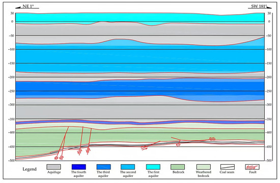
Figure 2.
Hydrogeological profile of the study area.
3. Data and Methodology
Aquifer water abundance prediction is divided into five steps: (1) First, drilling and geophysical survey data are collected. These data are then processed and analyzed to identify the key indicators for assessing aquifer water abundance; (2) The data for the water abundance factors were interpolated using the Ordinary Kriging method. This method employed a spherical variogram model, which was selected because it minimized the root mean square error in leave-one-out cross-validation, and a search neighborhood of 3 to 15 nearest points. Subsequently, the raster unit was designated as the evaluation unit. Finally, the spatial hierarchical structure of the evaluation indexes was constructed; (3) Aquifer water abundance is predicted using neural network models, such as the CPO-CNN-BiLSTM model; (4) The accuracy of different models is derived by comparing the predicted and actual values of unit water influx of aquifer; (5) This step applied the natural breaks classification method in ArcGIS 10.8 to zone the aquifer water abundance, utilizing both predicted and measured unit water influx values, enabling a direct comparative analysis of the outcomes. The research workflow is illustrated in Figure 3.
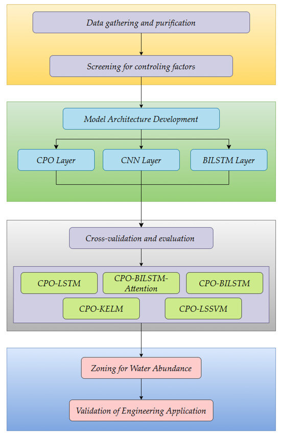
Figure 3.
The research workflow chart.
3.1. Analysis of the Main Evaluation Factors of Water Abundance
The factors affecting the water abundance of the loose fourth aquifer in the Quaternary System are multifaceted, and there is a close connection between the influencing factors. To effectively evaluate aquifer water abundance, this study, informed by prior studies, focuses on six controlling factors: aquifer thickness, gradation coefficient, marlstone thickness, grouting termination pressure, grouting quantity, and permeability.
The data of the main factors are derived from drilling, lugeon tests, pumping tests, real-time borehole orifice pressure monitoring, and other operations. Due to the difficulty in obtaining data and its scattered distribution, the spatial interpolation method was employed to derive more continuous and reliable information from limited datasets. Specifically, the Kriging interpolation technique was applied, and contour maps were generated for each control factor in the study.
3.1.1. Aquifer Thickness
The thickness of an aquifer is an intuitive reflection of the size of the water storage space. When all other conditions are equalized, the thickness of an aquifer is positively correlated with the amount of water stored. The greater the thickness, the greater the volume of groundwater contained in the formation, and the more water abundant it is. In terms of correlation, larger aquifer thickness is associated with higher porosity and permeability, which is favorable for groundwater storage and transportation.
Data on aquifer thickness are derived from borehole cataloging. By utilizing the borehole data, it is possible to determine the thickness of the aquifer at different points within the study area and apply the Kriging interpolation method to create a continuous spatial distribution to quantify the water storage potential of the aquifer. The thickness of the aquifers in the study area was mapped as shown in Figure 4a. As can be seen from Figure 4a, the aquifer’s thickness in the middle region of the study area is thinner than that in the northern and southern regions, with a thickness of 2.7 m–13.05 m.
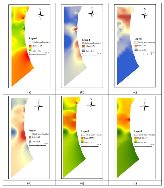
Figure 4.
Thematic map of evaluation factors. (a) Aquifer thickness; (b) Gradation coefficients; (c) Marlstone thickness; (d) Permeability; (e) Grouting quantity; (f) Grouting termination pressure.
3.1.2. Gradation Coefficients
Gradation coefficients can accurately reveal the distribution characteristics of large and small particles within an aquifer. When other influencing factors are kept constant, differences in soil particle size combinations can significantly affect the water abundance of an aquifer. The results of the pumping testing in the mining area show that the water abundance of the sandy strata with more gravel content is significantly stronger than that of the sandy strata with less gravel content. The water abundance of those with a larger grain size is better in the sandy and gravel strata. Loose-layer soil is weighted according to the particle size level to accurately quantify the influence of soil particle size combination on aquifer water abundance (as shown in Table 1). Then, this study constructs the particle size combination coefficient—grading coefficient D. The larger the value of D, the stronger the water abundance. It characterizes the strength of aquifer water abundance. D is calculated by the following formula:
where is the quantized value of grain size; is the thickness of soil layers with different grain sizes; and is the soil grain size category.

Table 1.
Results of assigning values to loose layers according to soil grain size classes.
Data on gradation coefficients are derived from borehole cataloging and lithological testing. Kriging interpolation creates a continuous spatial distribution, and ArcGIS maps the distribution of gradation coefficients in the study area, as shown in Figure 4b.
3.1.3. Marlstone Thickness
The development of the marl is more stable in the fourth aquifer. Generally, areas with a greater thickness of marlstone have relatively less water abundance. Because the marl is less permeable, it acts as a barrier to water seepage. The results of the water exploration and discharge experiments in the 85 mining district show that the unit water influx is smaller in the area with a larger thickness of marl. This observation indicates a negative correlation between marl thickness and aquifer water abundance. Additionally, the presence of marl will significantly affect the spreading and reinforcing effect of the grouting material, synergizing with the grouting material to improve the water insulation performance.
Data on marlstone thickness are derived from borehole cataloging. Kriging interpolation is used to create a continuous spatial distribution, and ArcGIS is used to map the distribution of marlstone thickness in the study area, as shown in Figure 4c. The thickness of the marl in the study area shows a decreasing trend from north to south, with a thickness of 0.09 m to 7.90 m.
3.1.4. Permeability
Permeability, a key indicator for describing aquifer infiltration performance, is quantified here in Lugeon values (Lu). Permeability is positively correlated with abundance. The greater the permeability, the stronger the water abundance. This parameter is closely related to the degree of rock fracture development, connectivity, and pore structure. A high permeability indicates less resistance to water flow and higher efficiency in groundwater transport.
The Lugeon value is obtained through the Lugeon water pressure test. During the test, conditions such as pressure, test section length, and internal diameter are strictly controlled to ensure the accuracy and reliability of the data, thereby accurately reflecting the permeability characteristics of the rock mass. French scholar Maurice Lugeon proposed this water pressure test method in the early 20th century. It defines a permeability of 1 Lu (Lugeon unit) as the injection of 1 L of water per minute into a 1-m-long borehole section under a pressure of 1 MPa [36]. In practice, the pressure and flow rate values from the maximum pressure stage are used to calculate the value according to the following formula:
where is the permeability of the test section (Lu); Q is the stable flow rate at the maximum pressure stage (L/min); L is the length of the test section (m); P is the pressure at the maximum pressure stage (MPa).
Kriging interpolation creates a continuous spatial distribution, and ArcGIS maps the permeability distribution in the study area, as shown in Figure 4d. The distribution of the permeability of the fourth aquifer before grouting is not uniform, and some areas are more permeable and relatively water abundant, posing a greater threat to safe mining. The difference between the maximum and minimum values is significant, and the variation ranges from 2.55 Lu to 11.76 Lu. The permeability is generally larger in the western and northwestern regions, whereas it is smaller in the eastern, northern, and part of the southeastern regions.
3.1.5. Grouting Quantity
The grouting quantity of a single hole visualizes the injectability and permeability of the formation around the corresponding hole. A large grouting quantity indicates that the formation’s initial pore and fissure development is better, and the permeability and water abundance are strong before and after grouting. The water abundance may still be retained at a relatively high level. Grouting treatment in the 85 mining district effectively reduced water permeability, particularly in boreholes with larger grouting quantity. However, it is still at a high level relative to the area with a small grouting quantity. The unit water influx is also relatively large, confirming that the grouting amount of a single hole is positively correlated to the aquifer water abundance after grouting.
Data on grouting quantity are derived from borehole grouting quantity statistics. Kriging interpolation is used to create a continuous spatial distribution, and ArcGIS is used to map the distribution of grouting quantity in the study area, as shown in Figure 4e. The grouting quantity exhibits a general decreasing trend from north to south and east to west, with notably lower volumes in some northern sectors. This spatial pattern is potentially linked to the heterogeneous distribution of factors such as marl thickness, with recorded grouting quantity ranging from 2.34 to 4757.01.
3.1.6. Grouting Termination Pressure
Grouting termination pressure visualizes the compactness and injectability of the formation. The higher the termination pressure of grouting, the weaker the water abundance of the formation. The slurry is injected into the strata under high pressure during grouting to block the pores and fissures. The flow resistance continues to rise, and the grouting pressure increases accordingly. A higher grouting termination pressure indicates effective sealing of permeable formation channels by the slurry, which significantly reduces the permeability coefficient and thereby leads to a marked decrease in water abundance. The inspection of the grouting effect shows that the area near the grouting boreholes with a higher termination pressure has a lower permeability rate. Thus, the grouting termination pressure is negatively correlated with water abundance.
Data on grouting termination pressure are derived from real-time borehole orifice pressure monitoring. According to the relevant specification requirements, the pressure sampling frequency is more than 1 time/30 s. Kriging interpolation is used to create a continuous spatial distribution, and ArcGIS is used to map the distribution of grouting termination pressure in the study area, as shown in Figure 4f. The range of grouting termination pressure in the study area is 0.016–10.19 MPa, with a decreasing trend from north to south.
3.2. Justification of the Chosen Evaluation Factors
In this study, selecting grouting water abundance influencing factors follows the triple criteria: data reliability, physical interpretability, and feature independence. All the parameters were obtained from hydrological boreholes, pumping tests, and core catalogs to ensure engineering applicability; the six parameters were directly related to the reservoir/conductivity mechanism of the formation through engineering evidence to avoid ambiguous indicators; and the highly correlated variables were eliminated through Pearson correlation analysis to ensure the independence of the model input features and the robustness of the prediction.
Additionally, porosity has not been used for two reasons. The grading coefficient directly quantifies the contribution of coarse particles (e.g., gravel) through the assignment of particle size and stratum thickness. As a parameter, it characterizes the pore structure, correlates directly with water abundance, and is strongly associated with porosity, thereby providing a comprehensive reflection of the aquifer’s hydraulic properties; Secondly, the grading coefficient can be quickly obtained through field data, addressing the sampling problem. It is more suitable for large-scale and low-cost hydrogeological investigations. This choice balances theoretical rigor and engineering practicality and provides an efficient solution for predicting the water abundance of weakly cemented strata. Correlation analysis is a statistical analysis method used to determine the size of the degree of correlation between two variables, its measurement index is the correlation coefficient (cr), the range of values −1.0 ≤ cr ≤ 1.0, the greater the absolute value of the cr, the higher the degree of correlation between the two factors, the negative value indicates negative correlation, the positive value indicates positive correlation. This study evaluates the degree of correlation between the control factors of water abundance by the Pearson coefficient method. The calculation results are shown in Table 2, and the correlation heatmap is shown in Figure 5.
Table 2.
Pearson’s correlation coefficients between control factors.

Figure 5.
Heat map of Pearson correlation between control factors.
The analysis shows that the termination pressure is moderately correlated with the marl thickness (r = 0.54) and the permeability with the gradation coefficient (r = 0.40); the rest of the parameters are weakly correlated with each other with |r| ≤ 0.31 (e.g., grouting volume and permeability r = 0.057). The correlation between the six parameters is below the high correlation threshold (|r| < 0.6), which meets the requirement of characteristic independence.
3.3. Evaluation Methodology
The modeling and computation in this study were conducted in the MATLAB (version R2023a) environment. The Deep Learning Toolbox was employed for constructing and training the CNN and BiLSTM networks. The optimization processes, including the implementation of the CPO algorithm and the hyperparameter tuning for the comparison models (LSSVM, KELM), were programmed utilizing the core functions and optimization utilities provided by MATLAB. This integrated software environment ensured the efficiency and reproducibility of all computational experiments.
3.3.1. Crowned Porcupine Optimization Algorithm (CPO)
The Crested Porcupine Optimizer (CPO), a novel swarm intelligence algorithm in 2024, automatically explores optimal hyperparameter spaces to overcome deep learning’s hyperparameter tuning challenge and enhance predictive efficiency [31]. The fundamental principle of the algorithm is inspired by the crested porcupine’s four defensive responses to predators. These four defense mechanisms correspond to distinct behaviors in the optimization process: the first two strategies emphasize global exploration for broad search-space investigation, while the latter two focus on local exploitation for intensive search within the most promising regions.
- (1)
- Stock initialization
During population initialization, each individual within the population represents a candidate solution, evaluated according to the objective function. The initial population is generated randomly within the search space, defined mathematically as:
where = 1, 2, …, N. N is the population size; is the position vector of the ith individual; rand is a uniform random number within [0, 1]; UB and LB are the upper and lower bounds of the search space, respectively. CPO incorporates a Cyclic Population Reduction (CPR) technique to decrease the population size periodically. This mechanism cyclically reduces the population scale (removing some individuals) and reintroduces new individuals in later iterations to enhance population diversity, thereby accelerating convergence. Its mathematical expression is:
where is the current iteration number; T is the number of cycles; % denotes the modulo operation. is the minimum size of the adjusted population, which is generally taken as 0.8 times of ; is the population size at the current iteration.
- (2)
- Exploratory Behavior Stage
During the exploratory behavior phase, the crown porcupine algorithm mimics visual and acoustic defense strategies against predators. This modeling of predator response can be used to navigate the search space and determine the best solution.
First defense strategy (visual): When a crowned porcupine encounters a predator, it raises and fans the spikes on its body to give the predator the impression that its body is more intimidating. At this point, the predator has a choice between backward and forward behavior. If the predator advances, the distance between them decreases, corresponding to the exploration phase in optimization, encouraging the search algorithm to investigate the region between the current position and the target, thus expediting convergence towards a solution. Conversely, if the predator retreats, it is forced to explore new, uncharted areas, reflecting a broad search strategy venturing into less explored or unvisited regions potentially containing superior solutions. This strategy simulates the process where individuals adjust their position based on the current best solution and stochastic information, aiming to balance convergence towards promising solutions with broader exploration. The position update is mathematically expressed as:
where is the position of the ith individual at iteration t; is the current optimal solution; is a random number based on the normal distribution; is a random number on the interval [0, 1]; is the position of the predator at t iterations, and the mathematical expression is:
where r is a random integer on the interval [1, N].
Second defense strategy (auditory): This strategy involves the crown porcupine deterring a predator by making noise when the predator is nearby. Predators will choose to approach, move away, or stand still. This strategy perturbs the current position using the difference vector of randomly selected individuals within the population, increasing search randomness and diversity. Its mathematical expression is:
where and are the positions of two distinct individuals randomly selected from the current population; is a random number on [0, 1]; is randomly taken to be either 0 or 1; and y is a reference position representing the baseline point for the perturbation direction, typically defined as the midpoint between the current individual and another randomly selected individual. When = 0, = , the individual’s position remains unchanged for this strategy in the current iteration, and when = 1, the individual’s position is updated based on the reference point y plus a scaled perturbation derived from the random difference vector . The direction of the difference vector determines the specific direction of the perturbation.
- (3)
- Developmental behavior stage
During this phase, crown porcupines use olfactory and physical attack strategies to respond to a predator’s approach. These strategies effectively facilitate spatial exploration, which leads to identifying the best solution.
Third defense strategy (olfaction): The crown porcupine releases a foul-smelling gas in its surroundings to deter predators from approaching. This strategy performs a more refined search near the current position by introducing a contraction factor and a random difference vector to control the search scope. The mathematical simulation is expressed as:
where r3 is a random integer located on the interval [1, N]; is a random number on [0, 1]; is a parameter controlling the search direction, defined by Equation (9); is a defense factor, defined using Equation (10); and is the Olfactory Diffusion Factor, typically valued within 0.3–2.6.
where t is the current number of iterations; is the maximum number of iterations. is used to simulate three possible scenarios: when = 0, the position is unchanged; when = 1, the position is undated.
Fourth defense strategy (physical attack): When a predator attacks, the porcupine resorts to a physical attack strategy. This strategy guides individuals towards the current global best solution , while introducing controlled random perturbations to avoid premature convergence. Its mathematical model draws inspiration from the concept of inelastic collision:
where is the convergence rate factor, typically set to 0.2; , are uniform random numbers within [0, 1]. is the perturbation term directed towards the optimum, calculated based on the principles of inelastic collision.
This study employs the Crested Porcupine Optimizer (CPO) for the automated tuning of hyperparameters within the CNN-BiLSTM model. CPO circumvents laborious manual intervention by efficiently searching for optimal hyperparameter combinations, thereby enhancing the model’s predictive accuracy and efficiency. Specifically, CPO optimizes three critical hyperparameters: the learning rate, the number of hidden units, and the L2 regularization coefficient. This optimization substantially enhances the performance of the CNN-BiLSTM model for tasks such as time series prediction and related applications.
3.3.2. Bidirectional Long Short-Term Memory (BiLSTM)
Long Short-Term Memory Networks (LSTM) are an evolved form of Recurrent Neural Networks (RNN). It combines gating mechanisms (specifically input, forget, and output gates) to overcome the challenges faced by traditional RNNs, such as gradient explosion and gradient vanishing. Water abundance prediction is a time series problem, relying on historical and future data. However, traditional LSTMs have limitations due to their unidirectional processing capabilities, restricting the ability to adequately capture forward time dependencies and hindering the utilization of future data. In contrast, BiLSTM overcomes this limitation by including two LSTM layers that process the input sequences in forward and reverse time order. This dual approach allows the BILSTM network to capture more comprehensive temporal information, thus improving prediction accuracy. The BiLSTM network architecture for this purpose is shown in Figure 6.
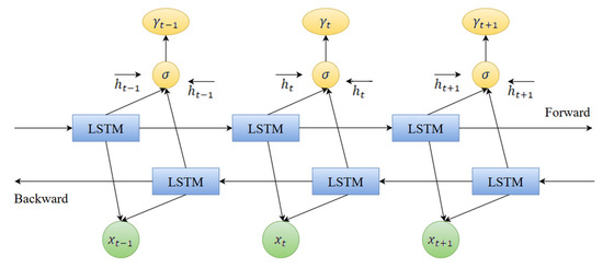
Figure 6.
Diagram of BiLSTM network architecture.
3.3.3. Principles of CPO-CNN-BiLSTM Modeling
CNN is a feed-forward neural network containing convolutional operations. Its implicit layers include convolutional, pooling, and fully connected layers, which realize the extraction, downscaling, and summarization of feature information of input data, respectively. Although this algorithm has a strong convolutional ability, it ignores the intrinsic connection between interrupted data. The BiLSTM network can also capture the data’s dependency between the before and after information.
Based on the spatial feature extraction capability of CNN and the bidirectional temporal feature extraction capability of BiLSTM, the two can be combined to construct a multilayer neural network, CNN-BiLSTM. This study achieves hierarchical extraction and synergistic modeling of spatiotemporal features through the deep integration of CNN and BiLSTM architectures. Within the feature extraction stage, a dual-level convolutional structure is used as the core spatiotemporal feature extractor. The primary convolutional layer employs 32 temporal convolution kernels of size [1 × 1], sliding along the temporal dimension with a stride of [1 × 1]. ‘Same’ padding is applied to preserve the temporal length of the feature maps. The secondary convolutional layer expands capacity to 64 [1 × 1] temporal kernels. This configuration extends the effective receptive field to 5 timesteps through a cascading effect, enabling the extraction of higher-order spatiotemporal features. Both layers incorporate ReLU activation functions to introduce non-linear decision boundaries and enhance feature representation capability. Features processed by the convolutional layers are reshaped into a sequential format via a sequence unfolding layer and compressed into a feature matrix by a flattening layer. This matrix is then fed into the BiLSTM module. The BiLSTM is configured with a hidden unit count optimized by the CPO, searching within the range of 5–100 units. Its gating mechanisms—namely the forget, input, and output gate–explicitly model long-term temporal dependencies. The forward LSTM processes the original temporal sequence, capturing evolutionary patterns from historical states, while the backward LSTM analyzes the sequence in reverse temporal order. The final hidden states from both directions are fused using end-step concatenation, effectively integrating bidirectional spatiotemporal dependency information.
The prediction accuracy of the CNN-BiLSTM model is affected by parameters such as initial learning rate, number of hidden layer nodes, etc. Hence, we use the CPO to optimize these parameters. A CPO-CNN-BiLSTM hybrid model is proposed to solve the problem of predicting aquifer water abundance by the influencing factors.
Its algorithmic flowchart is shown in Figure 7. Water abundance and its key evaluation factors are normalized and input into the CPO-CNN-BiLSTM hybrid model. A cross-validation strategy is used, where 80% of the normalized data is used for model training and the remaining 20% is used to test the model. Through multiple cycles of iterative training, the weights of each neural network layer gradually converge to the optimal state. Eventually, the hybrid model generates the water abundance predictions. Based on these outputs, the mean absolute percentage error (MAPE), root mean square error (RMSE), and coefficient of determination (R2) are calculated, serving as key evaluation metrics.
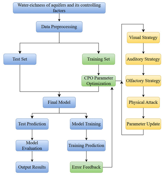
Figure 7.
Flowchart of the CPO-CNN-BiLSTM algorithm.
The CPO-CNN-BiLSTM is a multi-modal hybrid model that leverages the spatial feature extraction of CNN, the temporal modeling of BiLSTM, and the Cheetah Optimizer (CPO). This integration creates a powerful fusion of deep learning and intelligent optimization, with the complete prediction process detailed in Figure 7.
Firstly, after normalizing the data, including the unit water influx and six factors, the input dimensions of the prediction model are determined based on the number of delay times of the biased autocorrelation coefficient of unit influx. The dataset is divided into a training dataset and a testing dataset. Using randomly generated values for its BiLSTM hyperparameters (hidden layer nodes, initial learning rate, regularization coefficient), the initial CNN-BiLSTM model is constructed. The training dataset is then input to this model to yield the unit water influx predictions. RMSE of the prediction result is chosen as the fitness function of CPO to construct the optimal CNN-BiLSTM prediction model (CPO-CNN-BiLSTM point prediction model). The testing dataset is input into the CPO-CNN-BiLSTM point prediction model established in the second step to obtain the final prediction results. Finally, based on the predicted value of the unit water influx, we can expect the water abundance grade of the targeted aquifer.
4. Results and Discussion
4.1. Model Regulation and Running
The computational device used in this study is a Legion R9000P ARX8 computer, equipped with an AMD Ryzen 9 7945 HX central processing unit (CPU). This CPU features 16 cores and 32 threads, with a maximum boost frequency of 5.4 GHz and a performance release of up to 115 W. The model runs in the MATLAB environment, with a dataset consisting of 200 samples (For details, please refer to Supplementary Materials File S1), each containing six indicators. The total model training and evaluation runtime is 50 s, demonstrating its data processing efficiency. This computational resource ensures the rapid and efficient completion of the experiments.
To validate the performance and accuracy of the hybrid model, 200 groups (measured data included) of factor data are extracted from the contour plots plotted in the previous section, and each group included data from six control factors, which were used as a sample dataset. The sample dataset was partitioned into training and test sets. Robustness comparison experiments revealed that when the training set constituted 80% and the test set 20% of the data, the model exhibited significant superiority over conventional splits (e.g., training set ratios of 75%, 85%, and 90%) across key metrics. This included a 20.1% reduction in prediction error (RMSE) and a 73% decrease in distributional discrepancy (JS divergence). A Leave-One-Out Cross-Validation (LOOCV) strategy was employed on the 40 measured data points to address the concern regarding the non-independence of interpolated data and validate the model’s predictive capability at truly unseen locations. This method iteratively used 39 measured points (along with their associated Kriging-interpolated spatial fields) for training, while reserving the remaining single measured point for testing. This process was repeated 40 times, each time leaving out a different measured point. This ensures that the model is never evaluated on a point directly used to generate the training spatial field, thereby providing a strict and unbiased assessment of its generalization performance on independent data.
The study’s total sample is 200 groups of valid data samples, covering a range of 1.34 km2 in the 85 mining district. The data’s spatial resolution is a 50 m × 50 m grid, totaling 140 spatial cells. The data were collected from May 2020 to June 2024 (sampled monthly for 48 timesteps), and each sample contained six factors, as shown in Table 3.
Table 3.
Data features and sources.
The preprocessing procedure may be divided into four steps. Firstly, Missing value imputation: Based on Missing at Random (MAR) and Missing Not at Random (MNAR) diagnostics, spatial parameters (hydraulic conductivity, aquifer thickness) were imputed using Kriging interpolation, while temporal parameters (grouting volume) were imputed via BiLSTM predictive filling; Secondly, Outlier elimination: Local outliers were detected using an improved LOF algorithm (k = 15, LOF > 2.5), and global outliers were identified using Mahalanobis distance (95% confidence interval); Thirdly, Stratum-constrained normalization: Min-Max scaling was performed grouped by geological units; Finally, Spatiotemporal structuring: Normalized data were reshaped into a three-dimensional tensor [number of samples × timesteps × number of features] to meet CNN-BiLSTM input requirements.
The dataset consists of measured data in the field and data after kriging interpolation. The spatio-temporal characteristics of the data, such as spatial grid structure, time step, etc., need to be specified. Data preprocessing steps, such as normalization, missing value handling, and how to transform the data into a format suitable for model input, are also necessary. The first step is the hierarchical integration of data sources, which inputs different data sources through the core and derived data layers to achieve a more accurate preprocessing function. In the core data layer, we provide the measured field data (e.g., unit water influx, etc.) with 3D spatial coordinates (x, y, z) and time (t). In the derived data layer, the study provide continuous field data (permeability field, aquifer thickness contours, etc.) generated by Kriging interpolation, and allow the grid resolution to match the scale of variability of the geologic body. Finally, spatial local correlation construction and data enhancement strategies were applied to better meet the requirements of the CNN. Simultaneously, time-series structuring and long-range dependency guarantees were implemented to adapt the dataset to the temporal properties of the BiLSTM.
In the stage of building the neural network model, a blank network structure is created using the layerGraph function, network layers such as the Input-Layer, sequence folding layer, and convolutional layer are added, respectively, and the Connect-Layers function is used to connect the layers. The convolutional layer employs 1 × 1 kernels with 32 and 64 channels to enhance the interactive characterization of the six control factors via cross-feature fusion. This design intentionally avoids the use of 3 × 3 convolutions to preserve the integrity of temporal continuity. We use the Training Options function to set the training parameters, including the maximum number of iterations, the initial learning rate, the learning rate degradation factor, etc., which affect the stability of the model training and the length of training. The maximum number of iterations (epochs) is set to 100, the initial learning rate is 0.01, the learning rate decreasing factor is 0.5, and the learning rate decreasing period is 700. The dataset is disrupted at the beginning of each epoch, which helps the model generalize when learning and prevents the model from relying on a specific order of the data (For details, please refer to Supplementary Materials File S2).
CPO is used to automatically optimize three key hyperparameters of the CNN-BiLSTM model: learning rate, number of hidden units in BiLSTM, and L2 regularization. The specific parameters are set as follows: Population Size = 15, Max Iterations = 30, CPR cycles = 4, Minimum Population Size = 12, Convergence Speed Factor α = 0.2. The fitness function of CPO is defined as the root mean square error (RMSE) of the model’s prediction per unit of influx on the training set. With the efficient global search capability of CPO, the final optimal hyperparameter combination is determined as follows: the learning rate is 0.0087, the number of BiLSTM hidden units is 42, and the L2 regularization factor is 0.0001.
After training, the CPO-CNN-BiLSTM model has a root mean square error RMSE of 1.69 × 10⁻⁵ for the training set, 2.58 × 10⁻⁵ for the test set, and 1.90 × 10⁻⁵ for the overall RMSE, with a training dataset fitness of 0.982. To systematically verify the generalization ability, 5-fold cross-validation is used. The sample dataset is randomly divided into five subsets of equal size. Four subsets are used as the training set in turn, the remaining subsets are used as the training set in turn, and the remaining subset is used as the validation set; the training and validation are repeated 5 times. The average RMSE and R2 of the five validation sets were calculated. The results show that the average validation set RMSE =2.52 × 10⁻⁵ and the average R2 = 0.98, a slight deviation from the test set performance.
4.2. Water Abundance Prediction Zoning
The unit water influx predicted by the CPO-CNN-BiLSTM model is applied to assess the Cenozoic fourth aquifer. Zoning is then performed using the natural breaks method in ArcGIS (Figure 8a), with classification thresholds of 0.000479, 0.000605, 0.00077, and 0.001022. Based on these results, strong and medium-strong water abundance zones are found primarily in the eastern part of the study area, with smaller clusters scattered in the northwest and north. The distribution of strong water abundance aligns with areas of greater aquifer thickness, grouting quantity, and permeability, demonstrating a positive correlation with these factors. Conversely, it also coincides with zones of lower marlstone thickness and grouting termination pressure, indicating a negative correlation.
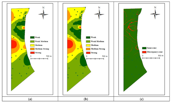
Figure 8.
The fourth aquifer water abundance zoning after grouting. (a) Water abundance zoning based on CPO-CNN-BiLSTM hybrid model; (b) Water abundance zoning based on measured unit water influx; (c) Discrepancy in water abundance zoning.
To validate the hybrid model’s reliability, the actual unit water influx values from the testing dataset were used to classify the water abundance. This classification was performed by applying the identical classification thresholds derived from the model’s predictions. As shown in Figure 8, the strong, medium–strong, medium–weak, and weak water abundance areas in the water-richness zoning maps plotted from the actual values of the unit water influx and the predicted values of the model’s testing dataset are slightly larger. Using ArcGIS’s reclassification tool and difference analysis tool, the discrepancy map between predicted and actual zoning can be obtained, as shown in Figure 8c. The map visually demonstrates that the areas with the greatest discrepancies are primarily concentrated in the northern part of the study area. This discrepancy may be attributed to the unevenness of grouting engineering. According to Figure 4e, the grouting quantity in the northern study area exhibits significant variation, where localized low grouting quantity failed to effectively seal aquifer channels, resulting in higher actual water abundance than predicted values. On the other hand, proximity to faults in the northern area may lead to more dynamic post-grouting hydrogeological behavior. Although BiLSTM can capture temporal dependencies, its response to sudden geological changes may exhibit latency. Still, the overall difference is minor, proving the model’s reliability.
The predictive uncertainty of the model was quantitatively assessed through a boot-strap resampling analysis (n = 1000 iterations) conducted on the 40 absolute prediction errors generated by the LOOCV procedure. This analysis yielded a 95% confidence interval (CI) for the RMSE of [2.21 × 10⁻⁵, 2.95 × 10⁻⁵]. The mean LOOCV RMSE (2.58 × 10⁻⁵) falls near the center of this confidence interval. This result statistically confirms that the model achieves a consistent and low level of prediction error when applied to truly independent and unseen spatial locations, effectively validating its generalization capability and reliability for aquifer water abundance evaluation.
4.3. Model Comparison Validation
The predictive performance of the CPO-CNN-BiLSTM model for water abundance was evaluated through a comparative analysis with other neural network models, including CPO-BiLSTM, CPO-LSTM, CPO-KELM, and CPO-LSSVM.
In the CPO-LSSVM model, CPO is used to optimize the coefficients and penalty coefficients of the Gaussian kernel function in the LSSVM [37]; In the CPO-KELM model, CPO is used to optimize the kernel parameters and penalty coefficients of the KELM [38]; In the CPO-LSTM model and CPO-BiLSTM model, CPO is used to optimize the number of hidden layer nodes, initial learning rate, and regularization factor of LSTM or BiLSTM. The prediction curves of the five prediction models are plotted against the proper value curves, as shown in Figure 9.
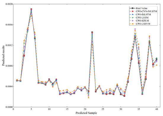
Figure 9.
Comparison of test set values with actual values.
As can be seen from Figure 9, the prediction curves of the five prediction models can also predict the unit water influx. Still, the prediction deviation near the peak and valley of the measured values is slightly larger. The error indices of the five prediction models, MAPE, RMSE, and R2, are shown in Table 4.
Table 4.
Forecasting method error indicators.
As can be seen from Table 2, the CPO-CNN-BiLSTM model has the lowest RMSE, indicating that the model has the least dispersion between the predicted and actual values. Integrated comparison of three error metrics of the five prediction models shows that the CPO-CNN-BiLSTM model has the highest prediction accuracy, followed by the CPO-BiLSTM model, the CPO-LSTM model, and the CPO-KELM model, respectively, and the CPO-LSSVM model has the lowest prediction accuracy. The statistical significance of CPO-CNN-BiLSTM’s performance superiority was evaluated using paired t-tests based on the absolute prediction errors from all 40 LOOCV folds. Statistically significant differences (p < 0.01) were confirmed against all other models, indicating that the performance improvement is robust and not due to chance.
The CPO-LSSVM and CPO-KELM models exhibit RMSE and MAPE values exceeding 5 × 10⁻⁵ and 6%, respectively, with an R2 below 0.903. In contrast, the CPO-LSTM, CPO-BiLSTM, and CPO-CNN-BiLSTM models achieve RMSE and MAPE values all below these thresholds (5 × 10⁻⁵ and 6%). This indicates that the prediction accuracy of the LSTM, BILSTM, and CNN-BiLSTM models based on a deep learning approach is better than that of the LSSVM and KELM models.
Comparison of three error metrics in the CPO-LSTM model, CPO-BiLSTM model, and CPO-CNN-BiLSTM model shows that the prediction accuracy of the CPO-BiLSTM model is better than that of the CPO-LSTM model, indicating that the BiLSTM network model has a higher prediction accuracy than the LSTM model. The prediction accuracy of the CPO-CNN-BiLSTM model is better than that of the CPO-LSTM model and the CPO-BiLSTM model, meaning that the combined model can effectively improve the prediction accuracy of a single model. In this study, the synergistic mechanism among the components of the CPO-CNN-BiLSTM model is profoundly revealed through different model comparisons. Removing the CNN module severely compromises spatial feature fusion capability, preventing effective extraction of deep nonlinear interactions within raw geological parameters. This forces BiLSTM to process low-discriminative features directly, increasing prediction error by 47.3%, whereas removing the CPO leads to the hyperparameter falling into a sub-optimal state, and the model has difficulty in balancing the fitting ability and the generalization, and the error may be even more significant. The synergistic nature of the two lies in the fact that the higher-order features extracted from CNN provide a smooth optimization space for CPO, while the precise tuning of CPO completely releases the potential of the CNN-BiLSTM architecture. This closed-loop “feature abstraction-parameter optimization” is precisely the core of the hybrid model’s performance that surpasses the performance of a single component.
Furthermore, the predictive performance of this model was benchmarked against state-of-the-art methods proposed in recent studies. For instance, Hou et al. [23] employed a WOA-SVM model to evaluate water abundance in weathered bedrock under similar hydrogeological conditions, achieving an RMSE of 3.58 × 10⁻⁵. Gai et al. [24] utilized a random forest model optimized through factor analysis, reporting an RMSE of 5.92 × 10⁻⁵ for their predictions. Xing et al. [25] implemented an NIPSO-SVM model with an RMSE of 4.81 × 10⁻⁵. In contrast, the CPO-CNN-BiLSTM model demonstrates a significantly lower RMSE (2.58 × 10⁻⁵), representing a 30% to 50% reduction in prediction error. This comparative analysis further underscores the exceptional performance of the proposed model for water abundance prediction in thick loose aquifers.
5. Conclusions
Combined with the characteristics of the study area, the aquifer thickness, gradation coefficient, marlstone thickness, permeability, grouting quantity, and grouting termination pressure are selected as the main factors of the aquifer for investigating the problem of water damage in the fourth aquifer after grouting. The reasonableness of the selection of evaluation indices is analyzed through correlation analysis. Then, the six factors are subsequently analyzed to predict the aquifer water abundance more accurately.
Average accuracy and root mean square error (RMSE) are used as model performance evaluation metrics. To ensure the robustness and credibility of the prediction, the first 160 sets of sample data were used as the training set of the model, and the remaining 40 sets of sample data (real data) were used as the test dataset. Two hundred sets of independent data were iteratively verified. They are fed into CPO-optimized machine learning models, such as the CPO-KELM, CPO-LSSVM, CPO-LSTM, CPO-BiLSTM, and CPO-CNN-BiLSTM hybrid models, to compare their respective prediction effects. The results show that the water richness prediction model based on the CPO-CNN-BiLSTM hybrid neural network has a higher accuracy and better prediction effect. In addition, each main control factor in the prediction model can be obtained in each construction borehole without geophysical exploration work, significantly reducing the construction cost.
After validation of the testing dataset, the predicted values of the model are highly fitted to the actual values, with the lowest MAPE (2.35%), the smallest RMSE (2.58 × 10⁻⁵), and the highest R2 (0.982). Using the predicted values of unit water influx, the water abundance of the fourth aquifer after grouting is classified, and it is found that the areas with higher water abundance are mainly distributed in the middle western and northern areas. Comparison with the zoning results of the actual value of the unit water influx reveals that the testing dataset in the hybrid model has high prediction accuracy, and the water abundance zoning coincides with the actual situation.
This study provides new insights for predicting the water abundance of thick loose aquifers and a theoretical basis for safe mining practices. Although the CPO-CNN-BiLSTM model shows high accuracy, its effectiveness is limited by the spatial representativeness of the training dataset, which may not fully capture regional hydrogeological heterogeneity. In addition, despite the rigorous selection of six key control factors, the potential impact of unquantified variables (e.g., fracture development density or fold undulation) remains to be explored, and the applicability of the model to different aquifer types, such as weakly cemented Jurassic aquifers, requires further validation. Future work should prioritize multi-mineral data integration, incorporating dynamic hydrological parameters, and cross-regional validation to enhance robustness.
Supplementary Materials
The following supporting information can be downloaded at: https://www.mdpi.com/article/10.3390/app152111816/s1, File S1: Sample data on 200 sets of control factors; File S2: CPO-CNN-BiLSTM program.
Author Contributions
Conceptualization, Y.L. and Q.W.; methodology, Q.W.; software, Y.L.; validation, J.Z., Y.L. and D.L.; investigation, Y.L.; resources, Q.W.; data curation, Y.L.; writing—original draft preparation, Y.L.; writing—review and editing, J.Z. and W.L. All authors have read and agreed to the published version of the manuscript.
Funding
This research was jointly funded by the National Natural Science Foundation of China (Grant Nos. 42007240 & 42372316).
Data Availability Statement
The original contributions presented in this study are included in the article. Further inquiries can be directed to the corresponding author.
Acknowledgments
The authors express their gratitude to everyone who assisted in the present study.
Conflicts of Interest
The authors declare no conflicts of interest.
References
- Yang, W.; Sun, W.; Liu, Y. Method and Prospect of Prediction and Evaluation of Mine Water Disaster in China. Coal Technol. 2019, 38, 115–117. [Google Scholar] [CrossRef]
- Noraishah Ismail, S.; Ramli, A.; Abdul Aziz, H. Research Trends in Mining Accidents Study: A Systematic Literature Review. Saf. Sci. 2021, 143, 105438. [Google Scholar] [CrossRef]
- Shao, Y.; Wu, Y.; Kang, F.; Zhu, S. Study on Seepage and Failure Characteristics of Soil at the Bottom of Thick Loose Layer in Thin Bedrock Area. Saf. Coal Mines 2025, 56, 203–211. [Google Scholar] [CrossRef]
- Chen, K.K.; Wang, X.Y. Analysis of the Factors Causing Roof Water Inrush in Coal Seam Mining with Thin Bedrock. Chem. Eng. Trans. 2015, 46, 679–684. [Google Scholar] [CrossRef]
- Sun, W.; Li, W.; Ren, L.; Li, K. Spatial and Temporal Characterization of Mine Water Inrush Accidents in China, 2014–2022. Water 2024, 16, 656. [Google Scholar] [CrossRef]
- Liu, Y.; Wu, Y.; Kang, F.; Zhu, S. Evaluation of Water Abundance of Loose Bed Bottom Aquifer. Saf. Coal Mines 2014, 45, 127–130. [Google Scholar] [CrossRef]
- Qiu, M.; Shao, Z.; Zhang, W.; Zheng, Y.; Yin, X.; Gai, G.; Han, Z.; Zhao, J. Water-Richness Evaluation Method and Application of Clastic Rock Aquifer in Mining Seam Roof. Sci. Rep. 2024, 14, 6465. [Google Scholar] [CrossRef]
- Miao, W.; Xu, Y.; Guo, Y.; Zhang, E.; Zhuo, Y.; Huang, L.; Ma, Z.; Liang, S. The Hydrogeological Characteristics of Thick Alluvium with High Water Level and the Influence on Zhaogu Mining Area, Henan Province, China. Geofluids 2022, 2022, 9447145. [Google Scholar] [CrossRef]
- Yang, W.; Hu, D. The Technology and It’S Application of Comprehensive Survey for Water-Bearing Condition of Fault. Coal Geol. Explor. 2002, 30, 51–53. [Google Scholar]
- Yan, S.; Wang, L.; Dong, F.; Liu, X.; Lu, X. Prediction of Burnt Rock Areas and Water Abundance Based on the Electrical-Magnetic Method. Coal Geol. Explor. 2022, 50, 132–139. [Google Scholar] [CrossRef]
- Cheng, J.; Zhao, J.; Dong, Y.; Dong, Q. Quantitative Prediction of Water Abundance in Rock Mass by Transient Electro-Magnetic Method with LBA-BP Neural Network. J. China Coal Soc. 2020, 45, 330–337. [Google Scholar] [CrossRef]
- Zhou, K. Water Richness Zoning and Evaluation of the Coal Seam Roof Aquifer Based on AHP and Multisource Geological Information Fusion. Geofluids 2021, 2021, 1097600. [Google Scholar] [CrossRef]
- Al-Abadi, A.M.; Pourghasemi, H.R.; Shahid, S.; Ghalib, H.B. Spatial Mapping of Groundwater Potential Using Entropy Weighted Linear Aggregate Novel Approach and GIS. Arab. J. Sci. Eng. 2017, 42, 1185–1199. [Google Scholar] [CrossRef]
- Li, Q.; Sui, W.; Sun, B.; Li, D.; Yu, S. Application of TOPSIS Water Abundance Comprehensive Evaluation Method for Karst Aquifers in a Lead Zinc Mine, China. Earth Sci. Inf. 2022, 15, 397–411. [Google Scholar] [CrossRef]
- Zhu, J.; Zhang, Y.; Li, W.; Wang, Q.; Ma, Z.; Li, X. Spatial Distribution Characteristics in Water Yield Property of Middle Jurassic Sandstone Aquifers Using Nonlinear Combination Method. Earth Sci. Inf. 2025, 18, 142. [Google Scholar] [CrossRef]
- Wu, Q.; Xu, K.; Zhang, W. Further Research on “Three Maps-Two Predictions” Method for Prediction on Coal Seam Roof Water Bursting Risk. J. China Coal Soc. 2016, 41, 1341–1347. [Google Scholar] [CrossRef]
- Wu, Q.; Fan, Z.; Liu, S.; Zhang, Y.; Sun, W. Water-Richness Evaluation Method of Water-Filled Aquifer Based on The Principle of Information Fusion with GIS: Water-Richness Index Method. J. China Coal Soc. 2011, 36, 1124–1128. [Google Scholar] [CrossRef]
- Hou, E.; Ji, Z.; Che, X.; Wang, J.; Gao, L.; Tian, S.; Yang, F. Water Abundance Prediction Method of Weathered Bedrock Based on Improved AHP and The Entropy Weight Method. J. China Coal Soc. 2019, 44, 3164–3173. [Google Scholar] [CrossRef]
- Ahmad, I.; Hasan, H.; Jilani, M.M.; Ahmed, S.I. Mapping Potential Groundwater Accumulation Zones for Karachi City Using GIS and AHP Techniques. Environ. Monit. Assess. 2023, 195, 381. [Google Scholar] [CrossRef]
- Yin, H.; Shi, Y.; Niu, H.; Xie, D.; Wei, J.; Lefticariu, L.; Xu, S. A GIS-Based Model of Potential Groundwater Yield Zonation for a Sandstone Aquifer in the Juye Coalfield, Shangdong, China. J. Hydrol. 2018, 557, 434–447. [Google Scholar] [CrossRef]
- Qu, X.; Han, J.; Shi, L.; Qu, X.; Bilal, A.; Qiu, M.; Gao, W. An Extended ITL-VIKOR Model Using Triangular Fuzzy Numbers for Applications to Water-Richness Evaluation. Expert Syst. Appl. 2023, 222, 119793. [Google Scholar] [CrossRef]
- Liang, K.; Li, Y.; Bai, Y.; Zhang, W.; Han, C.; Xie, D.; Liang, S.; Xi, B. Water-Richness Evaluation of Sandstone Aquifer Based on Set Pair Analysis Variable Fuzzy Set Coupling Method: A Case Study on Bayangaole Mine, China. Water 2025, 17, 1826. [Google Scholar] [CrossRef]
- Hou, E.; Wu, J.; Yang, F.; Zhang, C. Evaluation of Water-richness of Weathered Bedrock Based on the WOA-SVM Discriminant Model: Take Zhangjiamao Coal Mine in Shenfu Coal Field as an Example. Sci. Technol. Eng. 2025, 25, 119–127. [Google Scholar]
- Gai, G.; Qiu, M.; Zhang, W.; Shi, L. Evaluation of Water Richness in Coal Seam Roof Aquifer Based on Factor Optimization and Random Forest Method. Sci. Rep. 2024, 14, 24421. [Google Scholar] [CrossRef] [PubMed]
- Xing, M.; Wang, Q.; Xu, J.; Li, W. Application of NIPOS-SVM Model for Evaluation of Water Richness of Coal Seam Roof Aquifer—A Case Study of the Xinhu Coal Mine in Huaibei, China. Water 2024, 16, 3670. [Google Scholar] [CrossRef]
- Guo, B.; Zhang, S.; Liu, K.; Yang, P.; Xing, H.; Feng, Q.; Zhu, W.; Zhang, Y.; Jia, W. Prediction of Groundwater Level under the Influence of Groundwater Exploitation Using a Data-Driven Method with the Combination of Time Series Analysis and Long Short-Term Memory: A Case Study of a Coastal Aquifer in Rizhao City, Northern China. Front. Environ. Sci. 2023, 11, 1253949. [Google Scholar] [CrossRef]
- Panahi, M.; Sadhasivam, N.; Pourghasemi, H.R.; Rezaie, F.; Lee, S. Spatial Prediction of Groundwater Potential Mapping Based on Convolutional Neural Network (CNN) and Support Vector Regression (SVR). J. Hydrol. 2020, 588, 125033. [Google Scholar] [CrossRef]
- Qiao, L.; Xin, H.-C.; Xu, Z.-M.; Xiao, K. Gas Production Prediction Using AM-BiLSTM Model Optimized by Whale Optimization Algorithm. Appl. Geophys. 2023, 20, 499–506. [Google Scholar] [CrossRef]
- Zhang, C.; Liu, H.; Peng, Y.; Ding, W.; Cao, J. Intelligent Prediction and Application Research on Soft Rock Tunnel Deformation Based on the CPO-LSTM Model. Buildings 2024, 14, 2244. [Google Scholar] [CrossRef]
- Lin, Z.; Ji, Y.; Sun, X. Landslide Displacement Prediction Based on CEEMDAN Method and CNN–BiLSTM Model. Sustainability 2023, 15, 10071. [Google Scholar] [CrossRef]
- Abdel-Basset, M.; Mohamed, R.; Abouhawwash, M. Crested Porcupine Optimizer: A New Nature-Inspired Metaheuristic. Knowl.-Based Syst. 2024, 284, 111257. [Google Scholar] [CrossRef]
- Cheng, J.; Wang, H.; Xu, Z.; Huang, Q.; Jiang, G. Research on Aquifer Water Abundance Evaluation by Borehole Transient Electromagnetic Method Based on FCNN. Coal Geol. Explor. 2023, 51, 289–297. [Google Scholar] [CrossRef]
- Shi, S.; Shi, G.; Liu, Z.; Li, L.; Yao, X.; Pei, X.; He, Y. Predicting The Water-Yield Properties of K2 Limestones Based on Multivariate LSTM Neural Network: A Case Study of The Poil Mining Area in Yangquan. Coal Geol. Explor. 2023, 51, 155–163. [Google Scholar]
- Sang, S.; Lu, L. A Stock Prediction Method Based on Heterogeneous Bidirectional LSTM. Appl. Sci. 2024, 14, 9158. [Google Scholar] [CrossRef]
- Chen, S.; Cao, J.; Wan, Y.; Huang, W.; Abdel-Aty, M. A Novel CPO-CNN-LSTM Based Deep Learning Approach for Multi-Time Scale Deflection Basin Area Prediction in Asphalt Pavement. Constr. Build. Mater. 2025, 458, 139540. [Google Scholar] [CrossRef]
- Ding, L.F.; Guo, Q.L.; Wang, C.H. Lugeon water pressure test and its hydraulic friction in an oil reserve library project. Hydrogeol. Eng. Geol. 2011, 38, 35–38, 61. [Google Scholar] [CrossRef]
- Wang, H.Q.; Sun, F.C.; Cai, Y.N.; Ding, L.G.; Chen, N. An Unbiased LSSVM Model for Classification and Regression. Soft Comput. 2010, 14, 171–180. [Google Scholar] [CrossRef]
- Wang, Y.; Sun, X.; Wen, T.; Wang, L. Step-like Displacement Prediction of Reservoir Landslides Based on a Metaheuristic-Optimized KELM: A Comparative Study. Bull. Eng. Geol. Environ. 2024, 83, 322. [Google Scholar] [CrossRef]


Disclaimer/Publisher’s Note: The statements, opinions and data contained in all publications are solely those of the individual author(s) and contributor(s) and not of MDPI and/or the editor(s). MDPI and/or the editor(s) disclaim responsibility for any injury to people or property resulting from any ideas, methods, instructions or products referred to in the content. |
© 2025 by the authors. Licensee MDPI, Basel, Switzerland. This article is an open access article distributed under the terms and conditions of the Creative Commons Attribution (CC BY) license (https://creativecommons.org/licenses/by/4.0/).