Article

Mechanism and IPOA-ELM Predictive Modeling of Slippage in Traction Elevators

1
College of Quality and Standardization, China Jiliang University, Hangzhou 310018, China
2
Huzhou Special Equipment Inspection and Research Institute, Huzhou 313000, China
*
Authors to whom correspondence should be addressed.
Appl. Sci. 2025, 15(21), 11802; https://doi.org/10.3390/app152111802
Submission received: 25 September 2025 / Revised: 31 October 2025 / Accepted: 2 November 2025 / Published: 5 November 2025

Abstract

The reliable and safe operation of traction elevators depends on traction capacity, which is degraded by traction sheave groove wear. The resulting slippage reduces transmission efficiency and may cause a catastrophic failure due to the sudden loss of friction. After analyzing slippage mechanisms, we propose a prediction model that combines the Improved Pelican Optimization Algorithm (IPOA) with an Extreme Learning Machine (ELM). A mechanism analysis identifies key inputs—the wear amount, payload, and wire rope tension—providing a basis for model construction. The approach uses Halton sequence initialization, adaptive nonlinear weighting, and Gaussian perturbation, which improve the handling of nonlinearities. IPOA is then employed to optimize the ELM parameters, yielding the IPOA-ELM model. Experiments across multiple wear conditions show that IPOA-ELM predicts slippage more accurately than a traditional ELM. The study clarifies how traction sheave groove wear induces rope slippage and demonstrates the effectiveness of the proposed model under varying wear and load conditions, offering a practical reference for failure mechanism analysis and preventive strategies in elevator traction systems.

1. Introduction

Traction elevators, as safety-critical mechanical systems in modern urban infrastructure, represent the predominant vertical transportation solution globally, with their structural integrity directly impacting passenger safety and operational continuity. During actual operation, issues such as excessive wear on the traction sheave or uneven tension on both sides of the wire rope can reduce the friction between the sheave groove and the wire rope, leading to rope slippage [1]. Slippage of the wire rope not only reduces the transmission efficiency and safety of the elevator but may also lead to over-traveling or undershooting, resulting in severe personal safety accidents. However, the direct detection of traction sheave wear is challenging, and slippage is closely related to wear. Therefore, it is crucial to detect, predict, and analyze the slippage of elevator wire ropes to enhance safety and reliability.
As a critical failure mechanism in elevator mechanical systems, wire rope slippage has been extensively studied to prevent operational hazards and ensure structural integrity. Zhang et al. [2], using traction dynamics and friction transmission theory, found that relative slippage is caused by the tension difference between the two sides of the rope. Nakazawa et al. [3] developed a tension evaluation model considering rope slippage behavior, where simulation and experimental results clarified how increased sheave groove wear affects tension variation. Zheng et al. [4] investigated the fatigue life of elevator brake wheels under multi-field coupling effects, revealing the impact of thermal stress on mechanical failures, though their study did not address wire rope slippage dynamics. However, they assumed a uniform deceleration during braking, which deviates from real conditions. Chen et al. [5] proposed a non-contact measurement method that calculates rope slippage during braking using image detection techniques to assess the elevator traction capacity, though limitations in the marking range make it challenging to apply universally. Ma et al. [6] established a finite element model of wire rope with fiber and steel cores in contact with the traction sheave. Guo et al. [7] proposed a “global dynamic wrap-angle” theory unifying suspended and wrapped rope dynamics, showing vibration-induced dynamic slippage and friction-state reversals on the sheave. However, due to simplifications in the rope model and the discrepancy between the preload used in the simulation and the actual load in experiments, the simulation differed from actual operating conditions and lacked verification in real elevator systems.
The above studies provide valuable references for analyzing wire rope slippage; however, traditional physical models may face limitations when addressing the nonlinear and multivariable relationships inherent in complex dynamic systems. The Extreme Learning Machine (ELM) model, a feedforward neural network with a single hidden layer, offers advantages such as a fast learning speed and strong generalization capabilities [8,9]. It has been widely applied in fault prediction across multiple fields. For example, Shao et al. [10] proposed an intelligent diagnostic method for rolling bearing faults based on a Deep Wavelet Autoencoder (DWAE) with ELM, which eliminates the reliance on manual feature extraction and proves more effective than traditional methods and standard deep learning approaches. Yang et al. [11] introduced a novel EMD-ELM (Empirical Mode Decomposition ELM) multi-step prediction method, which is both highly accurate and easy to implement. Yaseen et al. [12] applied the ELM model to predict the compressive strength of foam concrete, demonstrating its potential through comparisons with Multivariate Adaptive Regression Splines (MARS), M5 tree models, and Support Vector Regression (SVR), thus reducing the need for labor-intensive trial batches to achieve the desired product quality. Kaloop et al. [13] developed a particle swarm-optimized ELM (PSO-ELM) to predict the resilient modulus of stabilized aggregate bases, improving the predictive accuracy over conventional ELM and ANN approaches. Ge et al. [14] developed a bat algorithm-optimized ELM (BA-ELM) for lithium-ion battery SOH estimation, improving accuracy over conventional ELM and other benchmark methods. Xiong et al. [15] developed a hybrid model for wind power forecasting, using BiLSTM and ELM models to predict high- and low-frequency components, resulting in an enhanced prediction accuracy.
Although the ELM model shows significant potential for applications across various fields, it still has limitations and drawbacks. Firstly, the weights and biases in standard ELM are highly random [16,17], introducing considerable uncertainty to the training accuracy and generalization capability. Additionally, to ensure effective learning and prediction under random initialization, a large number of hidden neurons are often required, which complicates the model [18]. Therefore, the primary goal of this study is to propose a novel optimization method for ELM model training that addresses the nonlinear, multivariable challenges of elevator slippage, thereby enhancing the prediction accuracy and robustness of the ELM model.
This paper proposes a slippage prediction model based on the Improved Pelican Optimization Algorithm (IPOA) and Extreme Learning Machine (ELM). The main contributions are as follows:
  • Through mechanism analysis, the relationships among traction sheave wear, traction capacity, and slippage amount are examined. Based on these analyses, key experimental design input parameters, such as wear amount, load capacity, and wire rope tension, are identified, providing a theoretical foundation for the subsequent model construction and optimization.
  • Improvements are made to the POA by introducing adaptive nonlinear weighting factors and Gaussian perturbations to significantly enhance the convergence and global optimization capabilities of IPOA. This enhancement not only improves the model’s stability with small sample data but also enables the more accurate adjustment of ELM parameters when handling specific conditions, such as severe wear or large tension differences, thus enhancing the slippage prediction accuracy. In contrast to the existing POA variants that mainly target the detection or avoidance of local extrema, the proposed IPOA further integrates a bounded sine-based adaptive weight with Halton sequence initialization and Gaussian perturbation. This design expands the effective exploration region in the early iterations while enforcing a controlled late-stage contraction, thereby mitigating premature convergence and yielding faster, smoother convergence under heterogeneous wear and load conditions. Combined with the mechanism-based slippage descriptors adopted in this study, these improvements strengthen robustness and reproducibility relative to prior POA-based approaches.
Compared with prior studies, physics-based traction models are often built on steady-state or idealized assumptions. They under-represent the nonlinear coupling among wear, load, and wrap angle, and they offer limited parameter identification and external validation. Many measurement or simulation schemes also have restricted applicability and provide little quantification of uncertainty. On the data-driven side, methods such as conventional ELM, ANN, and their variants are sensitive to random initialization and hidden-layer size, show a large variance across splits, and rarely include thorough ablation and reproducibility studies. These issues hinder stable generalization under small samples and strongly coupled conditions.
To bridge these gaps, we adopt mechanism-guided descriptors of equivalent friction, wrap angle and wear, and perform a focused parameter sensitivity analysis. We propose an improved IPOA-ELM in which Halton initialization, adaptive weighting, and Gaussian perturbation enhance the training stability and global search. Using repeated k-fold cross-validation, stronger baselines, and input-level sensitivity assessments, we demonstrate consistent gains in accuracy, robustness, and reproducibility.
The structure of this paper is as follows: Section 2 introduces the mechanism analysis of traction elevator slippage, identifying the influencing factors of slippage. Section 3 describes the principles of the basic algorithms and their improvements, including modifications to the Pelican Optimization Algorithm and optimizations for the Extreme Learning Machine. Section 4 discusses the design and implementation of the slippage experiments, followed by an analysis of the slippage prediction results under different wear conditions. Finally, Section 5 summarizes the main conclusions and findings of this study.

2. Analysis of the Mechanism of Traction Elevator Slippage

2.1. Traction Conditions of the Sheave Groove

The traction capacity is typically calculated using the Euler–Eytelwein formula, as shown below:
T 1 T 2 = e f θ
In Equation (1), T 1 and T 2 are the rope tensions at both ends, θ is the rope wrap angle, and f is the equivalent friction coefficient, as shown in Figure 1.
The traction capacity is determined by the frictional contact between the wire rope and the traction sheave. For a given traction system, the system’s operational status can be analyzed under three conditions based on the rope tensions [3]:
(1)
If T 1 T 2 < e f θ , the system has sufficient traction force and can operate normally.
(2)
If T 1 T 2   =   e f θ , the system reaches the critical traction force, and the wire rope may slip.
(3)
If T 1 T 2 > e f θ , the wire rope slips on the traction sheave, and the traction system is in an unsafe state.

2.1.1. The Impact of Traction Sheave Wear on Traction Capacity

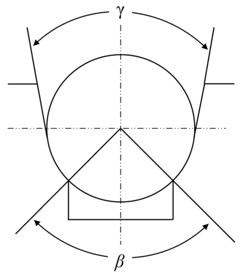
The impact of wear on traction capacity mainly occurs through changes in the geometric characteristics of the sheave groove, which further alter the equivalent friction coefficient, thereby changing the traction coefficient. A commonly used groove shape with a notched semicircular cross-section is shown in Figure 2. The key dimensions include the groove angle γ and the bottom notch angle β .
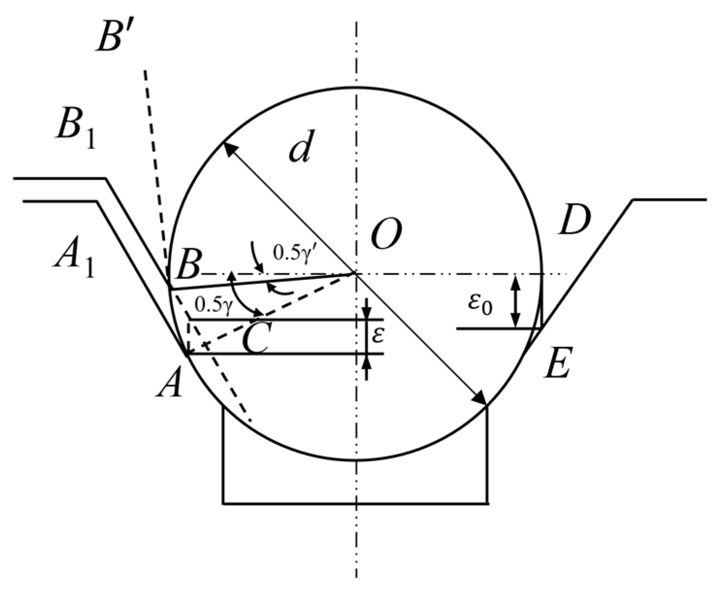
When the wear depth is ε , the center of the fitted circle of the groove arc is lowered by a distance of ε , which is equivalent to the rise of ε on the straight segment of the groove profile, as shown in Figure 3.
For the notched semicircular groove from the geometric relationship, d is the diameter of the fitted circle of the groove arc. After wear, the straight segment of the groove, A A 1 , changes to the position B B 1 , and the tangent point between the groove arc and the straight profile segment moves from point A to point B . The unworn groove angle is γ , while the worn angle is γ , and B B is the new tangent of the arc after wear. From the angular relationship, the following can be concluded:
A O B   =   0.5 γ 0.5 γ
cos A O B = 0.5 d A C 0.5 d = d 2 ε sin 0.5 γ d
By combining Equations (2) and (3), the relationship between the groove angle and the wear depth of the groove can be obtained as follows:
γ   =   γ 2 a r c c o s d 2 ε sin 0.5 γ d
In Figure 3, when the wear depth of the groove reaches ε 0 , the outermost point D of the fitting circle of the groove arc gradually wears down to the straight segment of the groove. At this point, the groove angle γ decreases to zero. After this, the groove continues to wear, but the groove angle γ does not change. The corresponding wear depth ε 0 is as follows:
D E   =   1 cos 0.5 γ sin 0.5 γ 0.5 d
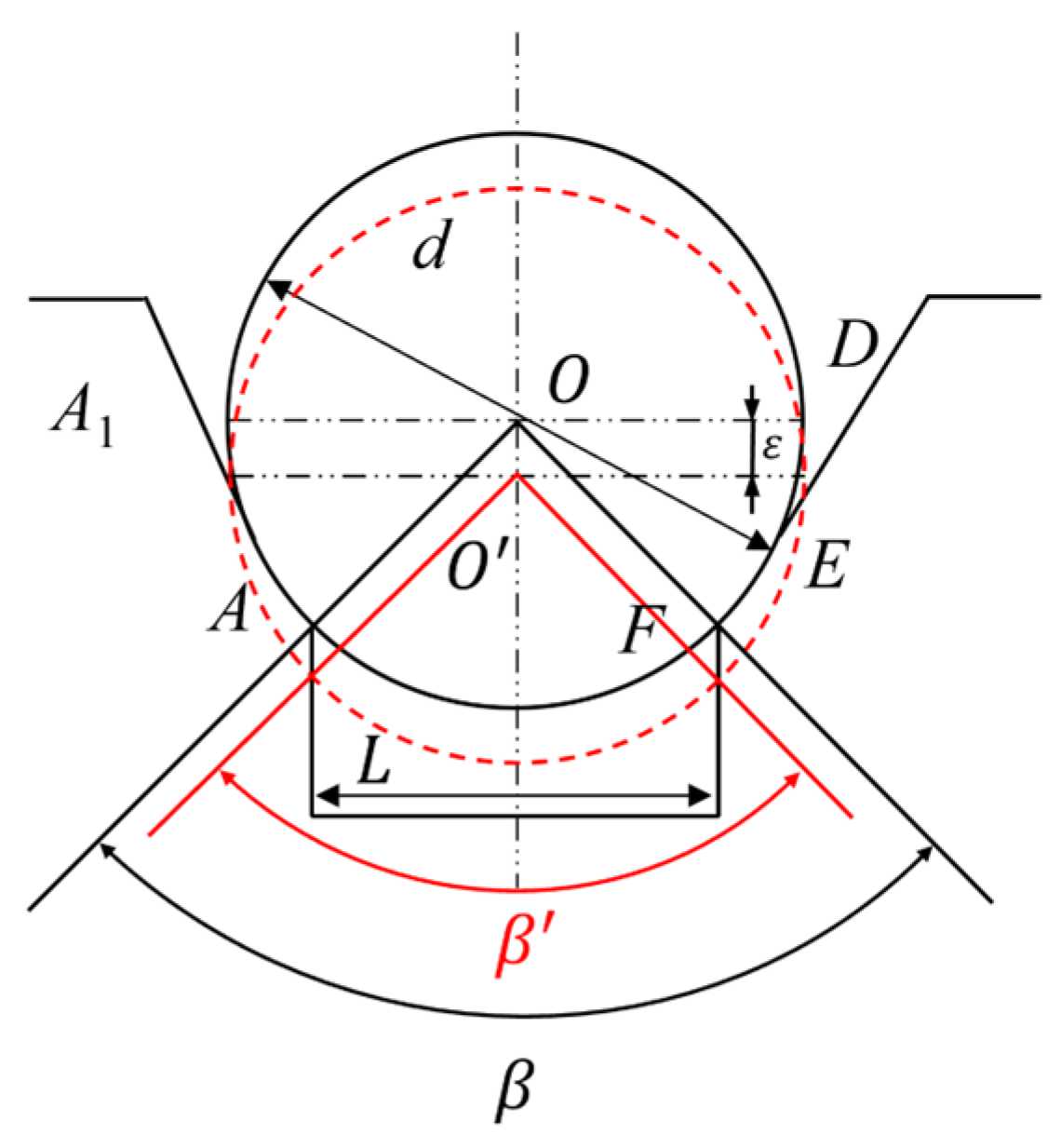
In Figure 4, β represents the initial notch angle of the notched semicircular groove, β denotes the notch angle of the notched semicircular groove after wear, and L is the notch width of the groove. It can be observed that the notch angle of the notched semicircular groove remains unchanged despite variations in the wear of the traction sheave.
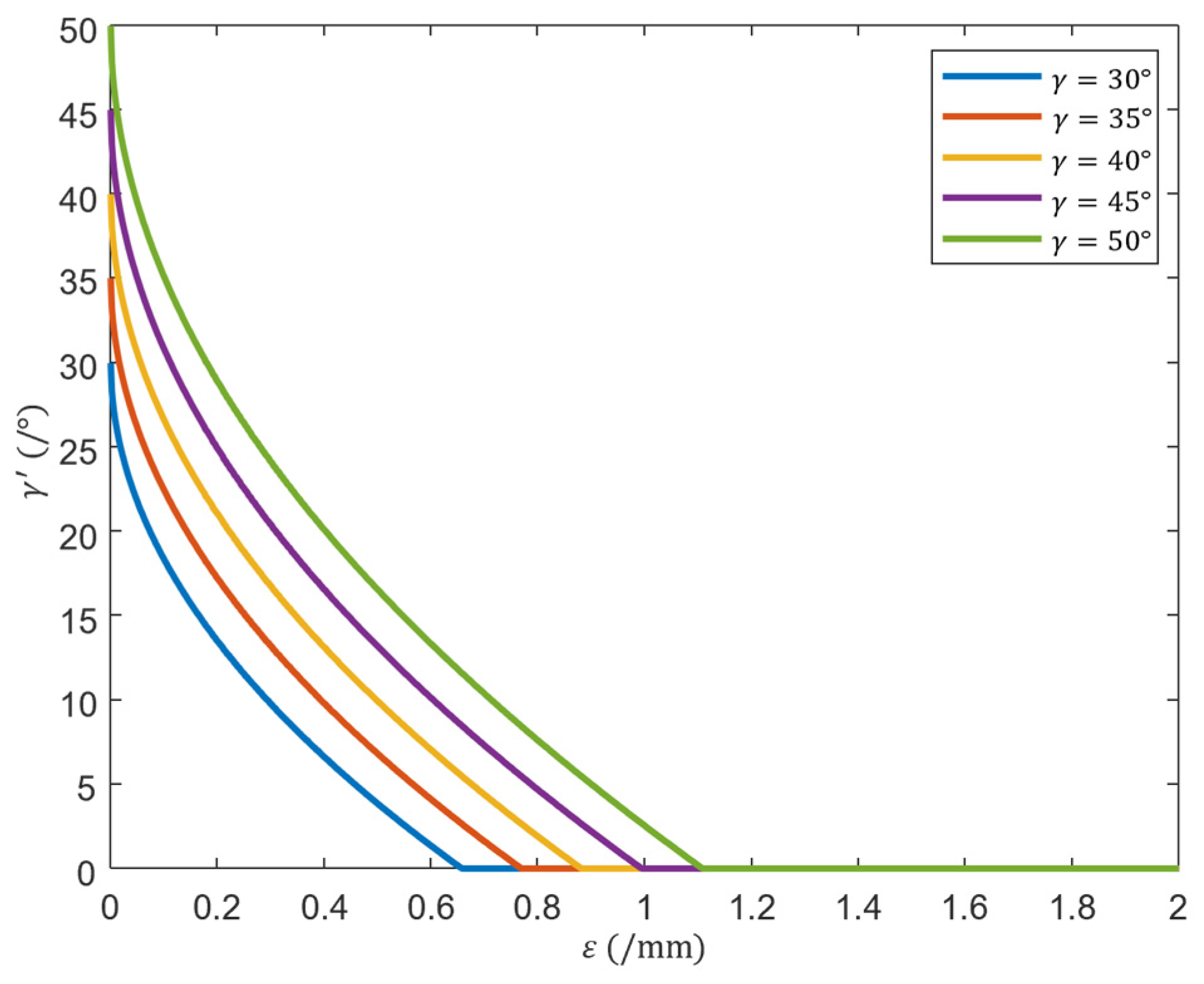
As an example, the variation in the groove angle with respect to wear is shown in Figure 5, with the initial groove angles γ set at 30 ° , 35 ° , 40 ° , 45 ° , and 50 ° . Semicircular grooves with notches are typically specified with a minimum initial groove angle γ of 25 ° . For a 10 m m diameter steel wire rope, the analysis indicates that a larger initial γ leads to a greater required wear depth ε 0 for the groove angle to be worn down to 0 ° .

2.1.2. The Relationship Between Groove Wear and Traction Capacity

The traction capacity of the groove depends on the equivalent friction coefficient and the wrap angle of the steel wire rope on the groove. The wear of the traction sheave has little effect on the reduction in the wrap angle and can be neglected, while the notch angle remains unchanged. For semicircular grooves with notches, the equivalent friction coefficient can be expressed as follows:
f   =   μ 4 ( c o s γ 2 s i n β 2 ) π β γ s i n β + s i n γ
here, μ represents the effective friction coefficient between the wire rope and the sheave groove under loaded steady-state conditions. This coefficient is not a material constant but varies with rope construction, lubrication status, wear level, contact pressure, and operating speed. On our test rig, the value was back-calculated as approximately 0.1 using data from the unworn baseline case, specifically the measured tension ratio and known wrap angle. Therefore, we adopt 0.1 as the representative value for subsequent analysis.
From Equations (1), (4), and (6), the traction capacity as a function of the equivalent friction coefficient and the wrap angle of the steel wire rope can be expressed as follows:
Z f , θ   =   e f θ
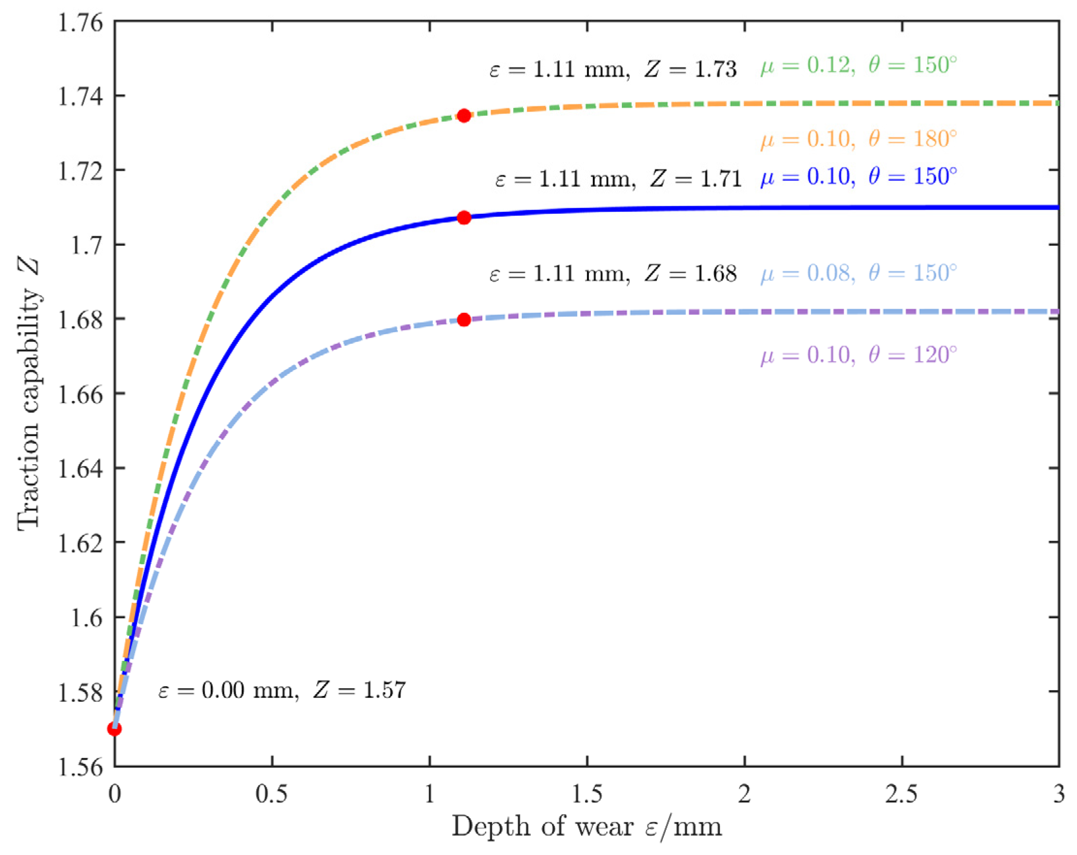
According to traction check provisions in elevator safety regulations, the required wrap angle follows the condition that links the tension ratio, the effective friction, and the angle. For the common semicircular groove with a notch, using a representative loaded-service friction of μ 0.1 and applying a safety factor of 1.2 to the worst-case tension ratio gives a minimum required wrap angle of about 150 ° ; we therefore take θ   =   150 ° degrees as a representative limiting configuration in the following analysis. Taking the wrap angle of the steel wire rope as 150 ° , the diameter of the fitted circle of the groove arc (steel wire rope) as 10 m m , the notch angle as 90 ° , and the initial groove angle as 50 ° before wear, the relationship between the traction capacity and wear depth under loading conditions is shown in Figure 6. The traction capacity increases with the wear depth, reaching a maximum of 1.71 when the wear depth reaches 1.11 mm, and then remains constant thereafter. To clarify the parameter sensitivity, Figure 6 overlays four reference curves. Increasing the effective friction at θ   =   150 ° from μ   =   0.10 to μ   =   0.12 or increasing the wrap angle at μ   =   0.10 from 150 ° to 180 ° raises the traction capability plateau from Z   =   1.71 to Z   =   1.73 and slightly steepens the initial rise. Conversely, reducing the friction to μ   =   0.08 at θ   =   150 ° or decreasing the wrap angle to 120 ° at μ   =   0.10 lowers the plateau to Z   =   1.68 and slows the approach to it. In all cases, the near-plateau onset occurs at ε   =   1.11 mm, indicating a limited benefit from additional wear. Taken together, μ   =   0.10 and θ   =   150 ° satisfy regulatory bounds while providing a stable and representative traction level with a reasonable convergence rate. They avoid over-conservatism under higher friction or larger wrap angles and insufficiency under lower friction or smaller wrap angles, and are therefore adopted as the baseline for subsequent analyses.

2.2. Analysis of the Slippage Mechanism

In traction elevators, slippage refers to the relative displacement between the traction sheave and the steel wire rope caused by an insufficient traction capacity due to factors such as contact friction between the wheel groove and the rope. This represents a transition from a state of relative rest to sliding between the two contact surfaces [6]. As shown in Figure 7, slippage is defined as the difference in marked distance over one complete round-trip, representing the amount of slippage between the traction sheave and the steel wire rope. The analysis that follows is purely analytical in nature and does not employ any dedicated simulation platform or numerical solver.
During elevator operation, the amount of slippage can be classified into elastic slippage and abnormal slippage. In the constant-speed phase, elastic slippage primarily occurs due to small deformations between the steel wire rope and the traction sheave, which can be calculated theoretically. However, during the acceleration and deceleration phases, the system’s dynamic changes are more significant, making abnormal slippage more likely. Such slippage must be detected and analyzed using real operational data to determine whether it exceeds the normal range.

2.2.1. Analysis of Slippage in Uniform Motion

According to the Euler–Eytelwein theory, the formula for calculating the relative velocity of the steel wire rope on the traction sheave is as follows:
v x   =   T 1 T 2 E A v z
In Equation (8), E is the elastic modulus of the steel wire rope ( N / m m 2 ) , A is the cross-sectional area of the steel wire rope, v z is the operating speed of the steel wire rope ( m m / s ) , and v x is the relative slippage speed of the steel wire rope ( m m / s ) .
T 1 T 2 = M D M J n r
In Equation (9), M D represents the counterweight mass and M J represents the elevator car mass, which includes both the car’s own weight Q z and the car’s load Q J . n is the number of strands of the steel wire rope, and r is the traction ratio.
Since, during the uniform motion, the tension difference on both sides of the traction sheave remains constant, the relative sliding acceleration α x of the steel wire rope also remains unchanged.
t = l v z
In Equation (10), t represents the time ( s ) from when the steel wire rope begins to contact the traction sheave until it leaves contact with the sheave, and l is the contact length ( m m ) between the traction sheave and the steel wire rope.
Therefore, the elastic slippage of the steel wire rope during the uniform motion phase is as follows:
L   =   1 2 α x t 2 H   =   H 2 n E A M D M J
In Equation (11), H   ( m m ) represents the distance traveled by the elevator.
Through the above analysis, we can calculate the elastic slippage during the elevator’s uniform motion phase, which is primarily related to the material properties of the steel wire rope, the contact length, and the load difference. Equation (11) describes only the elastic slippage during the constant-speed phase and is used as a physics reference in the traction analysis. In this paper, the response variable for prediction is the total slippage per run measured by the encoder in millimeters, which equals the elastic component plus the contributions that arise during acceleration and deceleration and from changes in the friction state.

2.2.2. Analysis of Slippage During Acceleration and Deceleration Phases

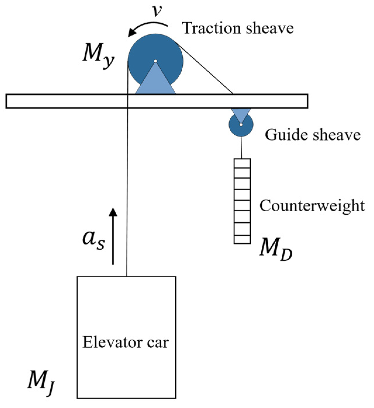
The relative slippage between the traction sheave and the steel wire rope occurs because the elevator’s traction capacity is less than the maximum static friction force between the sheave and the rope, resulting in slippage. To calculate the relative slippage, a mechanical model of the elevator car under a heavy load during the downward braking process, as shown in Figure 8, is established.
In Figure 8, v   ( m m / s ) represents the rotational speed of the traction sheave; a s   ( m m / s 2 ) is the average acceleration of the steel wire rope and the elevator car and counterweight assembly; and M y   ( k g ) is the mass of the traction sheave.
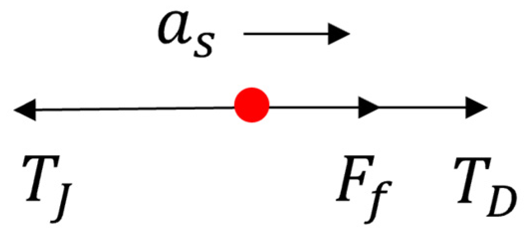
The force analysis for the traction sheave and the steel wire rope is shown in Figure 9 and Figure 10. In these diagrams, a z   ( m m / s 2 ) represents the braking acceleration of the traction sheave, F z   ( N ) denotes the braking force, F f   ( N ) is the frictional force, T D is the tension on the counterweight side ( N ) , and T J   ( N ) is the tension on the elevator car side.
During the heavy-load downward braking process of the elevator car, a force analysis is conducted separately for the traction sheave, the combined system of the elevator car and counterweight, and the individual components of the car and counterweight. Due to the presence of acceleration at the traction sheave, the tension on both sides of the wheel differs, resulting in varying accelerations. The acceleration on the car side is denoted as a J , and the acceleration on the counterweight side is denoted as a D (calculated as scalars, without considering direction):
F z F f   =   M y a z M D g n + F f M J g n   =   ( M D + M J ) a s T J M J g n   =   M J a J M D g n T j   =   M D a D
In Equation (12), g n denotes the standard gravitational acceleration. During the heavy-load downward braking process of the elevator car, the braking force F z overcomes the frictional force F f between the traction sheave and the wire rope, providing a braking acceleration a z for the traction sheave. As the braking force F z increases, the relative motion tendency between the traction sheave and the wire rope also increases, leading to an increase in the frictional force F f . The frictional force F f provides the acceleration a s for the wire rope, elevator car, and counterweight system as a whole. However, when the friction becomes insufficient to impart the same acceleration to the wire rope, car, and counterweight as that of the traction sheave, relative sliding occurs between the sheave and the rope, resulting in excessive slippage. Therefore, the greater the required balancing force, the more likely the frictional force F f will exceed the maximum static friction limit, causing an increase in slippage between the traction sheave and the wire rope.
From Equation (12), the frictional force between the traction sheave and the wire rope during the heavy-load downward braking process can be expressed as follows:
F f   =   ( M D + M J ) a s + ( M J M D ) g n
Similarly, the operating conditions most likely to cause excessive slippage include heavy-load downward braking, heavy-load upward acceleration, light-load upward braking, and light-load downward acceleration.
Based on the Euler formula for frictional transmission, we can derive the following:
F f   =   M D ( g n a s ) ( e f θ 1 )
From Equations (13) and (14), the following can be derived:
a s   =   M D e f θ M J M D e f θ + M J g n
Based on the above analysis, the slippage amount during the downward braking phase can be calculated as follows:
L z   =   v 0 2 2 a s v 0 2 2 a z   =   1 2 v 0 2 2 M D e f θ M J M D e f θ + M J g n v 0 2 2 a z
In summary, during the heavy-load downward braking process, the excessive slippage of the elevator is related to the cabin load and the coefficient of friction, which in turn is influenced by the wear of the sheave groove.
The monitoring of wire rope slippage is critical for fault prediction related to traction sheave wear, as abnormal slippage often indicates potential failure risks in the elevator sheave. By accurately measuring the slippage, it is possible to proactively identify wear-induced faults in the sheave, prevent impaired traction performance, and mitigate safety hazards, thereby enhancing the operational reliability and efficiency of the elevator system. However, wear-induced slippage typically exhibits complex nonlinear characteristics that are difficult to capture accurately with conventional linear theoretical models. To address this challenge, machine learning methods are introduced to predict abnormal slippage. This approach effectively compensates for the limitations of theoretical analysis and provides a more robust technological foundation for predicting traction sheave failures.

3. Slippage Prediction Method of Wire Rope Based on IPOA-ELM

3.1. Extreme Learning Machine Network

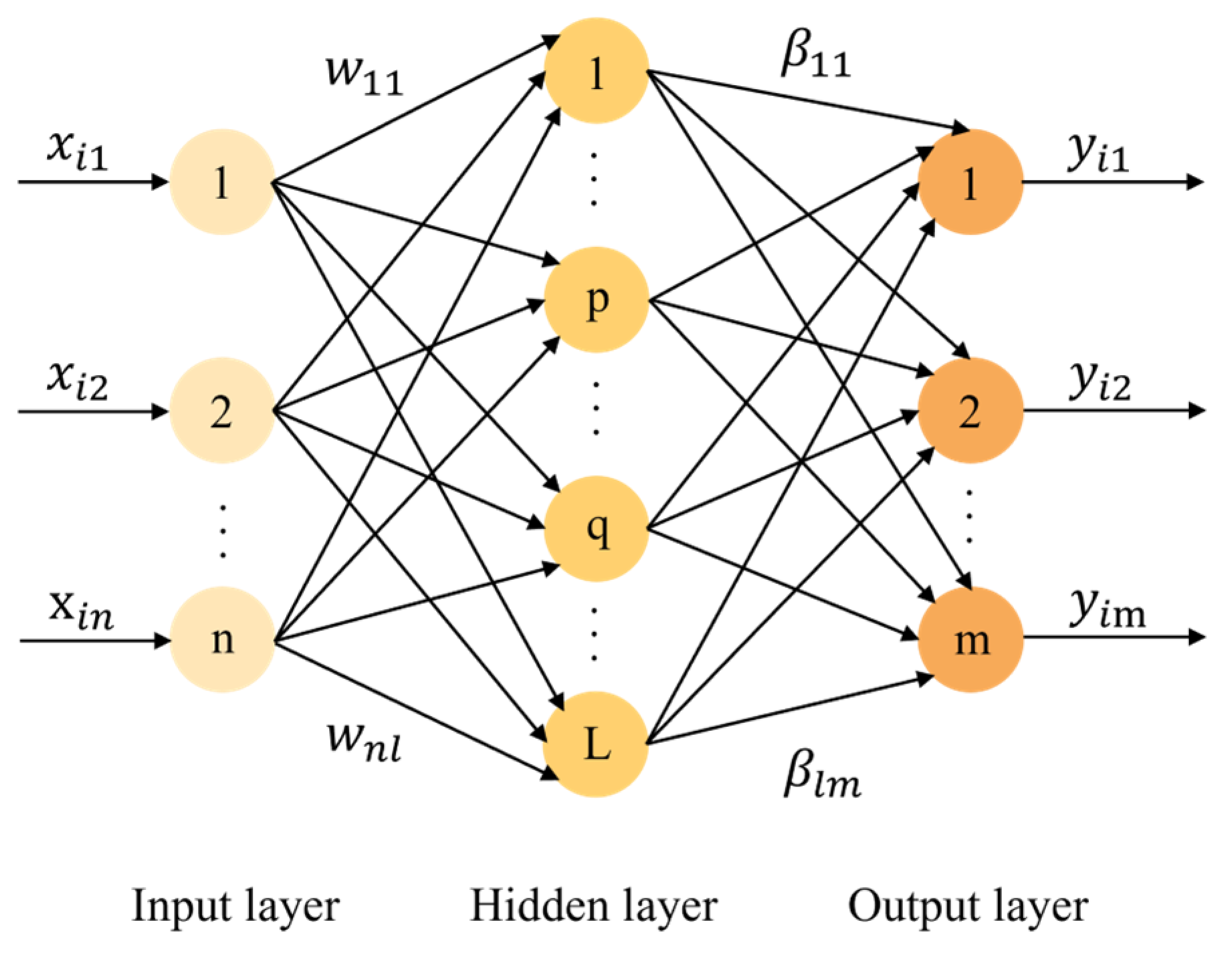
The Extreme Learning Machine (ELM) [19] is a fully connected single-hidden-layer feedforward neural network, and its architecture is shown in Figure 11.
In Figure 11, n , L , and m denote the numbers of neurons in the input, hidden, and output layers, respectively. Let a dataset consisting of N input–output pairs be denoted as E = { ( x i , y i ) } i   = 1 N . For the i -th sample, the input vector is x i = ( x i 1 , x i 2 , , x i n ) T , and the actual output vector is y i = ( y i 1 , y i 2 , , y i n ) T . For the i -th sample with input features x i , the k -th component of the ELM output is the following:
j   = 1 L β j k g ( w j T x i + b j ) = y ^ i k
In Equation (17), g · denotes the activation function of the hidden-layer neurons; y ^ i = y ^ i 1 , y ^ i 2 , , y ^ i m is the network output vector of the i -th sample; w j = w j 1 , w j 2 , , w j n T is the input weight vector of the j -th hidden neuron; b j is the bias of the j -th hidden neuron; and β j = β j 1 , β j 2 , , β j n T denotes the weight vector from the j -th hidden neuron to the output layer.
Equation (17) can be expressed in matrix form as follows:
H β   = Y
In Equation (18), β   = β 1 , β 2 , , β L T is the connection weight matrix between the hidden-layer neurons and the output-layer neurons; Y   = y 1 , y 2 , , y N T denotes the wire rope slippage; and H is the hidden-layer output matrix, as shown in Equation (19):
H = g w 1 T x 1 + b 1     g w L T x 1 + b L                                                       g w 1 T x N + b 1     g w L T x N + b L N × L
The training of ELM can be formulated as a least-squares problem for the output weight matrix β :
β ^   =   H Y
In Equation (20), H denotes the Moore–Penrose pseudoinverse of H .

3.2. Pelican Optimization Algorithm

The Pelican Optimization Algorithm (POA) was first introduced by Pavel Trojovsky in 2022 [20]. It primarily consists of two stages: the exploration phase and the exploitation phase.
(1)
Exploration Stage
q u , v P 1 = q u , v + r a n d p v I q u , v , F p < F u q u , v + r a n d q u , v p v , e l s e
In Equation (21), q u , v P 1 represents the new position in the v -th dimension for the u -th pelican after the first stage of updating; p v is the position of the target in the v -th dimension; F p denotes the target function value; I is a random integer, taking either 1 or 2; and r a n d is a random number within the interval [ 0,1 ] . If the target function value is improved at this new position, the position is accepted; otherwise, it is not accepted.
Q u =                   Q u P 1 , F u P 1 < F u Q u , e l s e
In Equation (22), Q u P 1 represents the updated position of the u -th pelican, and F u P 1 denotes the objective function value corresponding to the first stage.
(2)
Exploitation Stage
q u , v P 2 =   q u , v + R 1 t T 2 · r a n d 1 q u , v
In Equation (23), q u , v P 2 represents the position of the u -th pelican in the v -th dimension after the second stage update. Here, R   = 0.2, and R 1 t T represents the neighborhood radius of q u , v P 2 , where t is the current iteration count and T is the maximum number of iterations. The term r a n d represents a random number uniformly distributed in the interval 0,1 . If the updated objective function value is improved, the new position is adopted.
Q u =                   Q u P 2 , F u P 2 < F u Q u , e l s e
In Equation (24), Q u P 2 represents the updated position of the u -th pelican, and F u P 2 denotes the objective function value for the second stage.

3.3. Improved POA-ELM Algorithm

3.3.1. Population Initialization Based on Halton Sequence Mapping

In the POA, random population initialization can yield insufficient diversity, reducing the search efficiency and slowing convergence. We therefore adopt a Halton sequence initialization generated with pseudo-random numbers [21]. Owing to its good space traversal, the Halton sequence increases the initial diversity and strengthens the global exploration, which is particularly beneficial for our small-sample slippage dataset. As a result, the solutions reach promising regions earlier and the algorithm converges faster with improved accuracy.
For a two-dimensional Halton sequence, the mathematical model for the partitioning process, using two prime numbers as the base, is as follows:
n   =   i   =   0 m b i · p m + + b 1 · p 1 + b 0
θ n = b 0 p 1 + b 1 · p 2 + b m · p m 1
H n = θ 1 ( n ) , θ 2 ( n )
In Equations (25)–(27), n represents the index of the Halton sequence; p is a prime number greater than or equal to 2; b i 0,1 , , p 1 are constants; θ ( n ) is a defined sequence function; and H ( n ) denotes the resulting two-dimensional Halton sequence.
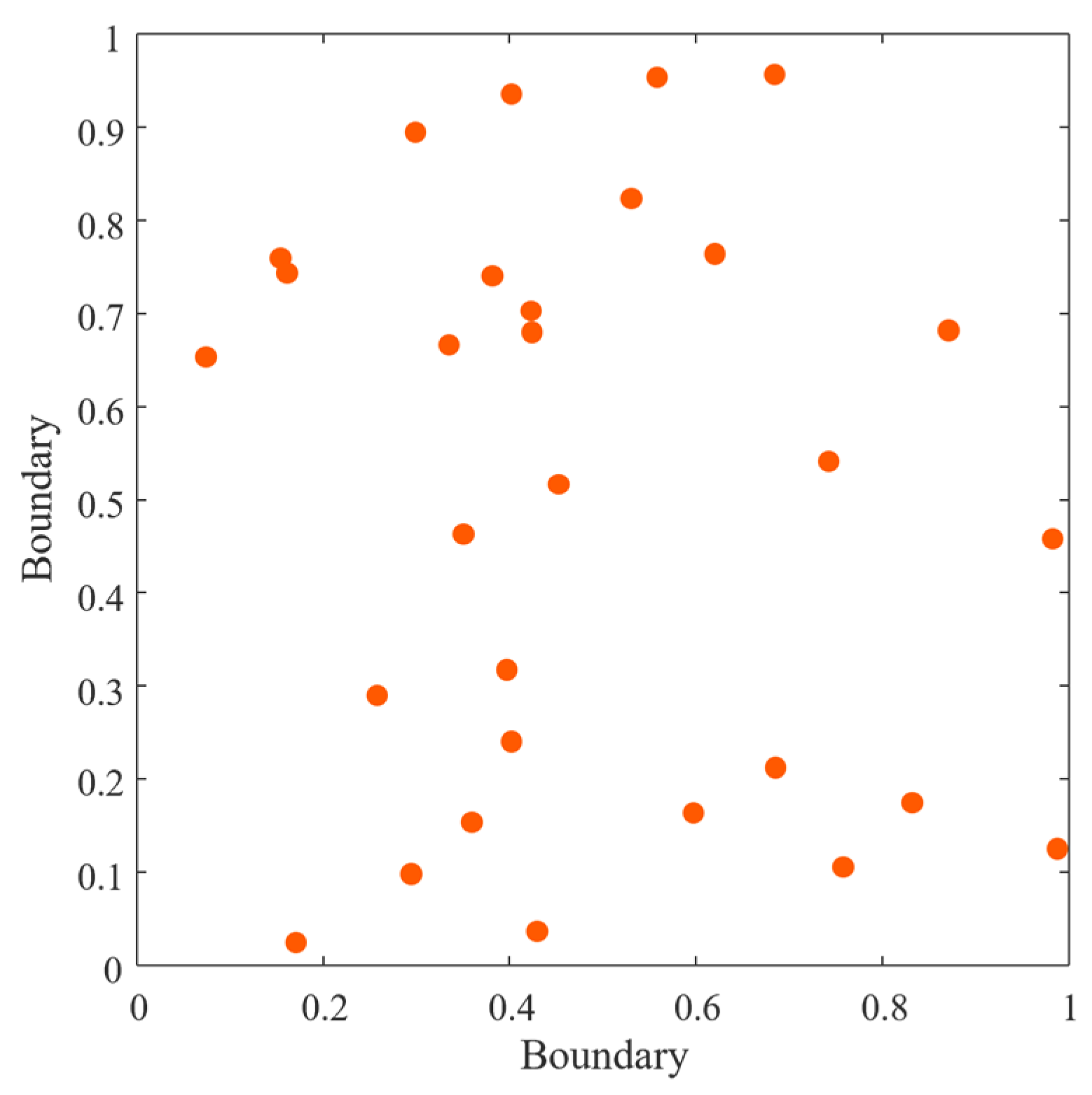
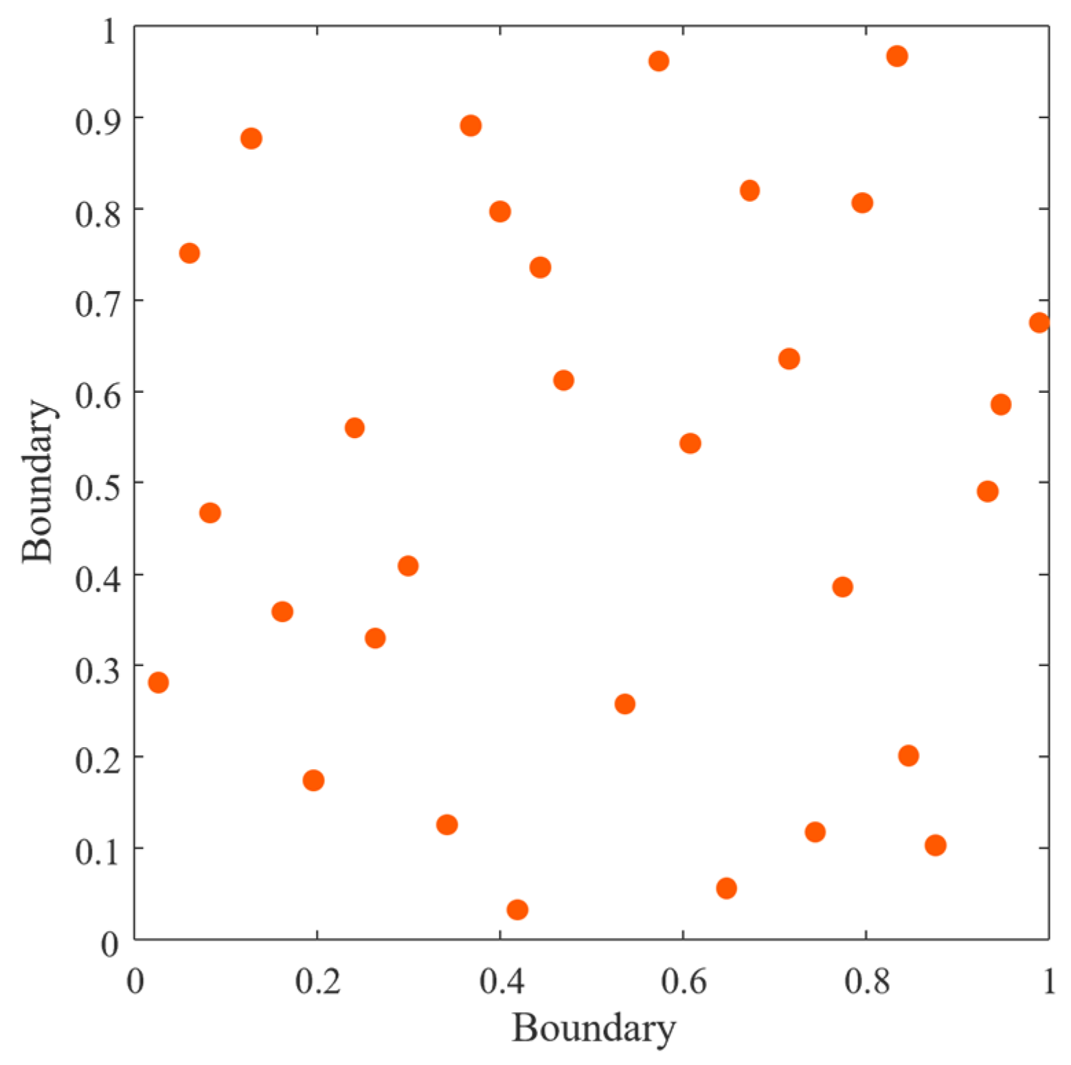
Figure 12 and Figure 13 visualize the population distributions generated by the POA under random initialization and Halton sequence initialization, with the Halton base numbers set to 2 and 3. The Halton-based populations provide broader and more uniform coverage with reduced overlaps and fewer gaps, ensuring a better exploration of the search space. Consequently, the POA more efficiently locates optima across multiple regions, improving its global optimization capability.

3.3.2. Adaptive Weight Factor

In the second phase of the Pelican Optimization Algorithm, the presence of the linearly decreasing term 1 t T as the iteration progresses leads the algorithm to converge too quickly to a local optimum. This issue becomes more pronounced when dealing with slippage datasets under limited operating conditions, which may not reflect real-world scenarios. Consequently, the predictive accuracy of the model is affected. To address this, an inertia weight was introduced to improve the algorithm’s tendency to prematurely converge and fall into local optima during the later stages of iteration [22]. To further resolve this problem, an adaptive nonlinear weight factor based on a sine function is introduced, with the following expression:
w   =   w m a x ( w m a x w m i n ) · sin t / T μ · π / 2
In Equation (28), w m a x = 0.9 ; w m i n = 0.2 ; and μ   = 2 .
The adaptive weight governs the update magnitude. The upper bound w m a x determines the initial step scale; the lower bound w m i n determines the terminal step scale; and the shape parameter μ controls the sine-based decay curve. We set w m a x   =   0.9 to retain a near-full search capability at the start, while keeping updates strictly bounded; w m i n   =   0.2 ensures a small but non-vanishing terminal step that suppresses noise amplification and prevents stagnation. With μ   =   2 , the schedule exhibits a smooth decay with a pronounced mid-run decrease, allocating most iterations to exploration and the closing part to refinement. Under { 0.9 ,   0.2 ,   2 } , relatively large weights persist through about the first sixty percent of iterations, whereas very small weights are confined to the final twenty percent, implementing the intended search-then-refine regime.
This setting remedies the weakness of a linear schedule in phase two: larger early steps curb premature convergence, while bounded late steps yield a stable, non-overshooting refinement. By dynamically adjusting the weight, the exploration–exploitation balance remains consistent across wear and load levels, adapting the search to varying conditions and improving the exploration of slippage under diverse operational scenarios.

3.3.3. Gaussian Perturbation

To prevent entrapment in local optima, a zero-mean Gaussian perturbation is applied to the best-performing pelican at each iteration [23], as given in Equation (29). This maintains population diversity, broadens the exploration of the search space, and thereby accelerates convergence and improves accuracy.
Q u , n e w =   Q u + G a u s s i a n μ , σ 2
In Equation (29), Q u , n e w represents the updated position, G a u s s i a n ( · ) denotes the Gaussian function, μ is the mean, and σ 2 is the variance.
When the population converges near a certain solution, Gaussian perturbation can further explore local optima, especially in scenarios with severe wear or significant tension differences. This enhances prediction accuracy and ensures the model’s adaptability and accuracy under various operating conditions.

3.4. Development of the IPOA-ELM-Based Wire Rope Slippage Prediction Model

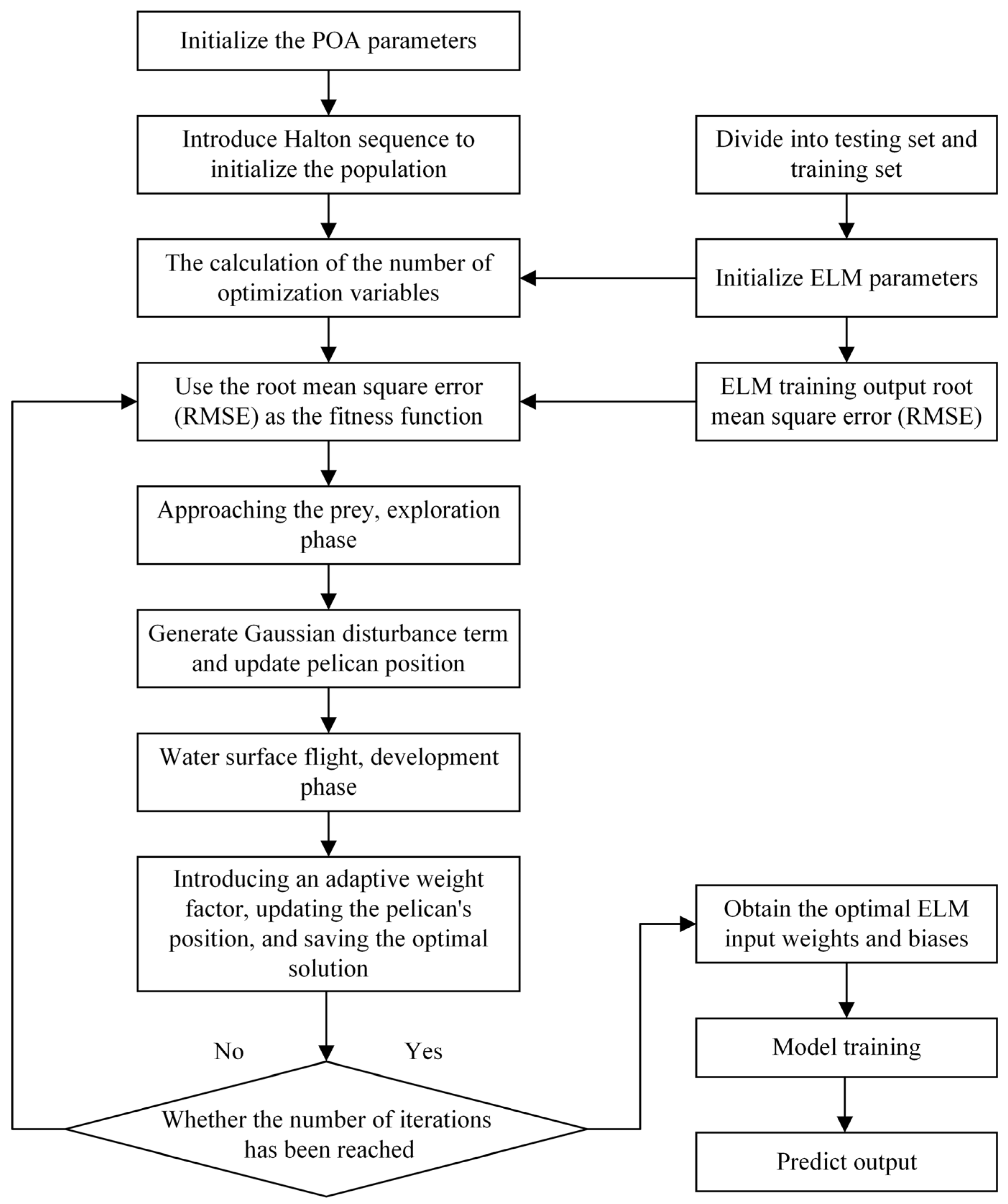
The improved Pelican Optimization Algorithm (IPOA) is employed to optimize the Extreme Learning Machine (ELM). Within a limited number of iterations, the optimal training sample weights and hidden-layer biases are obtained, ensuring the best regression prediction performance of the ELM. This optimization process effectively overcomes the instability in regression prediction caused by the random initialization of parameters in traditional ELM, thus improving the accuracy of the steel wire rope slippage prediction model. The optimization process is shown in Figure 14.
The specific steps for optimizing the weights and biases of the ELM (Extreme Learning Machine) using the Improved Pelican Optimization Algorithm (IPOA) are as follows:
  • Step 1: Normalize the slippage test dataset. The test data include the wear, load, and tension (T1, T2) of the wire ropes on both sides of the traction sheave, and slippage. To obtain a robust estimate of the generalization performance, we employed repeated k-fold cross-validation. The complete dataset was partitioned into k folds of approximately equal size. During each iteration, one fold was designated as the test set, with the remaining k 1 folds forming the training set. We configured k   =   10 and performed R   =   10 repetitions, ensuring that each sample was included in the test set multiple times under varying data partitions. This methodology effectively reduces the variance associated with individual random splits and yields a more stable and reliable estimation of prediction error.
  • Step 2: Set the number of hidden-layer nodes L of the ELM to 10, choose the Sigmoid activation function, set the pelican population size N to 30, and set the maximum number of iterations T to 100.
  • Step 3: Initialize the pelican population positions using Equation (27), where each pelican’s position represents the weights and biases of the ELM.
  • Step 4: Substitute the experimental data and the pelican positions into the ELM prediction model, using the Root Mean Square Error (RMSE) of the prediction model as the fitness value. The calculation formula is as follows:
    f x   =   1 M i   =   1 M Y i y i 2
In Equation (30), M represents the number of samples; Y i is the true value of the sample; and y i is the predicted value of the sample.
  • Step 5: Use Equations (21) and (22) for exploration updates and apply Equation (29) for Gaussian perturbation.
  • Step 6: Use Equations (23) and (24) for exploitation updates, with the adaptive weight defined in Equation (28).
  • Step 7: If the current iteration count t   <   T , repeat steps 4 to 6. If the maximum iteration count is reached, terminate the iteration.
  • Step 8: Output the best individual position, which represents the weights and biases of the Extreme Learning Machine (ELM). Then, establish the IPOA-ELM slippage prediction model and perform error analysis and evaluation.

4. Discussion

4.1. Test Data Collection

The data used in this study were collected from an elevator testing base. The subject of the research is a traction-driven freight test elevator with a machine room. The basic parameters of the elevator are shown in Table 1 below:
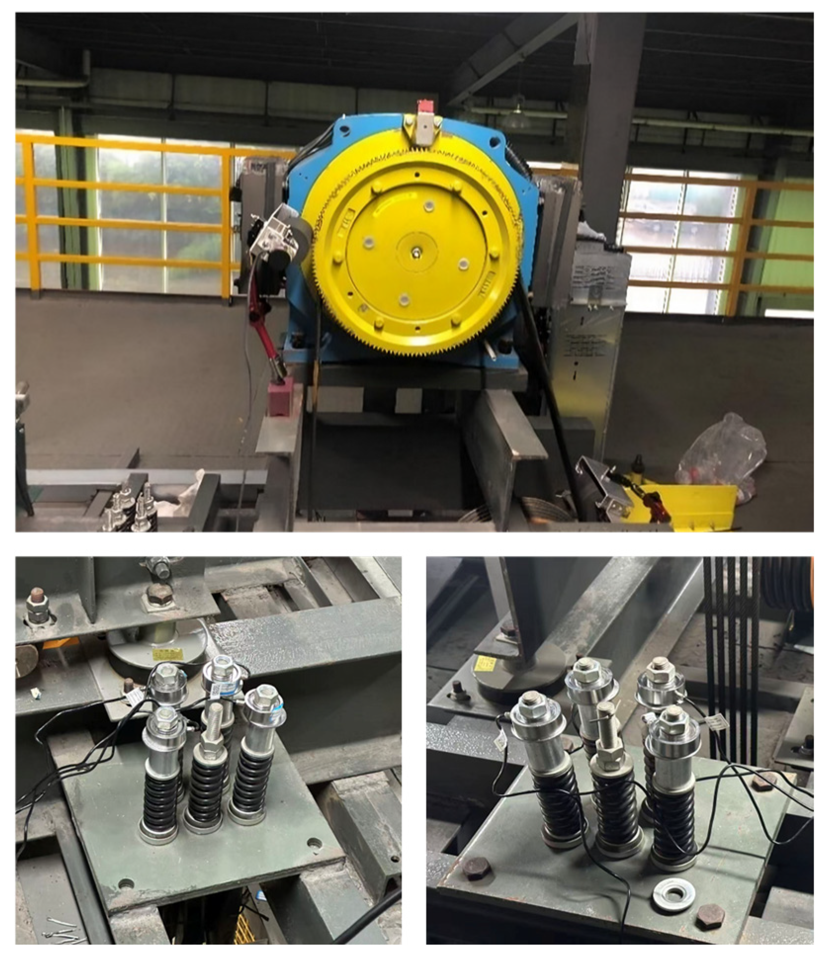
An in-depth investigation of wire rope slippage was conducted. The traction sheave groove was machined through uniform circumferential cutting with a forming tool to simulate the radial groove wear caused by wire rope friction during service. Wear conditions were graded from no wear to rope-bottom contact, and round-trip tests were performed for each wear level under different payloads. JHBM 4 model load cells with a range of 0 to 500 kg and a sensitivity of 0.00245 mV per N were installed at each rope termination to measure the tension of each rope, and the signals were recorded by an IM1208H data acquisition unit with ten channels at 1024 Hz per channel under a common trigger and a shared time base with the encoder; the tensions on the same side were summed to obtain the total tensions on the two sides, T1 and T2. Before testing, the load-cell chain was calibrated with traceable deadweights at five levels from zero to full scale, with ascending and descending runs repeated three times. A least-squares fit was used to obtain the gain and zero corrections, and nonlinearity, hysteresis, and repeatability were recorded. For each operating condition, we conducted ten round-trips and used the mean as the final measurement, and the repeatability across the ten trips was used to estimate the measurement uncertainty. Slippage was acquired using a dual-channel integrated encoder device that we independently developed. The device is based on the conversion method principle. The dual-channel integrated encoder synchronously measures the traction sheave angular displacement and the wire rope linear displacement, converts the former to linear travel using the measured sheave diameter, and computes the slippage as the difference between the two over a given time interval, while acquiring and streaming data in real time. It delivers a resolution of 0.1 mm and achieves a measurement accuracy above 90% over the tested range. The experimental setup is shown in Figure 15.
Equation (11) computes only the elastic slippage during the constant-speed stage; the slippage subsequently used for prediction in this paper is the encoder-measured total slippage per run, which, in addition to that elastic component, includes slippage arising from acceleration and deceleration as well as from changes in the friction state. One run is defined as a full round-trip from the bottom floor to the top and back. For each operating condition, we averaged the net slippage over ten round-trips. During the data collection process, all reported values corresponded to this ten-trip average. A total of 82 datasets on wire rope slippage were collected, and model training and evaluation used repeated k-fold cross-validation with k equal to 10 and R equal to 10, where the data are divided into k approximately equal parts and each part serves once as the test set. A portion of the slippage data obtained from the test is shown in Table 2.

4.2. Comparison Models and Evaluation Metrics

To comprehensively compare the performance of the improved POA-optimized ELM elevator wire rope slippage prediction model, the following evaluation metrics were selected: Mean Absolute Error (MAE), Root Mean Square Error (RMSE), the Coefficient of Determination ( R 2 ), and the Mean Absolute Percentage Error (MAPE). A superior model performance is indicated by concurrently lower MAE, RMSE, and MAPE, coupled with a higher R 2 . The formulas for calculating each evaluation metric are as follows:
M A E =   1 M i   =   1 M S i S ^ i
R M S E = 1 M i = 1 M S i S ^ i 2
R 2 = 1 i = 1 M S i S ^ i 2 i = 1 M S i S ¯ i 2
M A P E = 1 M i = 1 M S i S ^ i S i × 100%
In Equations (31)–(34), S i represents the measured total slippage per run, S ^ i represents the predicted value, S ¯ i represents the mean value of the sample, and M is the number of samples.

4.3. Prediction Results Analysis

To validate the accuracy of the proposed Improved Pelican Optimization Algorithm-Optimized Extreme Learning Machine (IPOA-ELM) in predicting wire rope slippage, comparative experiments were conducted. In addition to the Pelican Optimization Algorithm-Optimized Extreme Learning Machine (POA-ELM) and the traditional Extreme Learning Machine (ELM), we further included three representative baselines: Support Vector Regression (SVR) with a Gaussian radial basis function kernel, XGBoost, and linear regression using physically meaningful variables. The 82 sets of elevator experimental data were preprocessed and split using k-fold cross-validation for training and evaluation.
In each split of the repeated k-fold cross-validation, the IPOA was employed for iterative training to determine the optimal position of the pelican, which corresponds to the optimal weights and biases of the Extreme Learning Machine (ELM). The Root Mean Square Error (RMSE) was used as the fitness function, and the fitness curve of the Improved IPOA-ELM optimization is shown in Figure 16. As shown, the algorithm reached the global optimum after 18 iterations, demonstrating a relatively fast convergence rate.
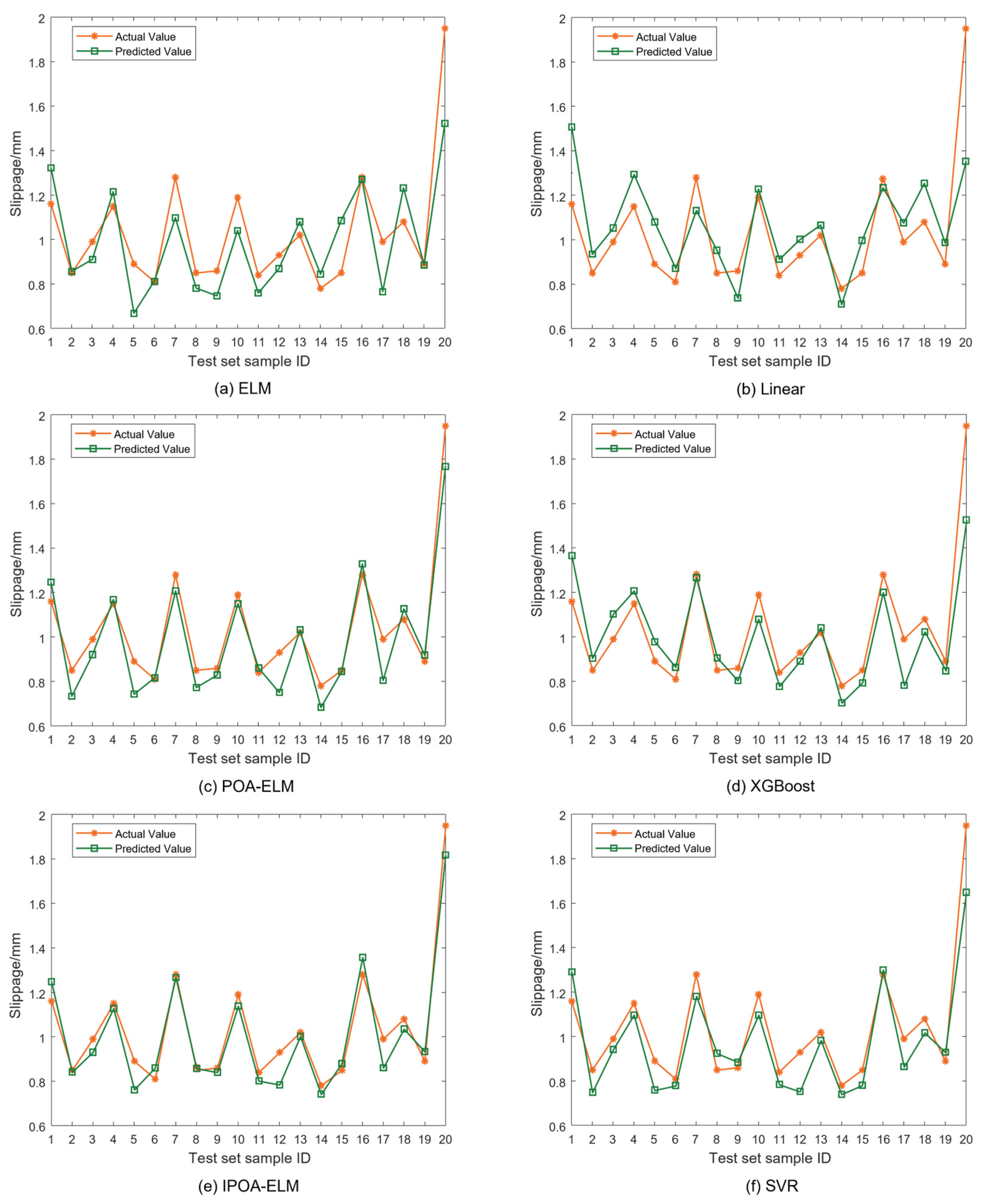
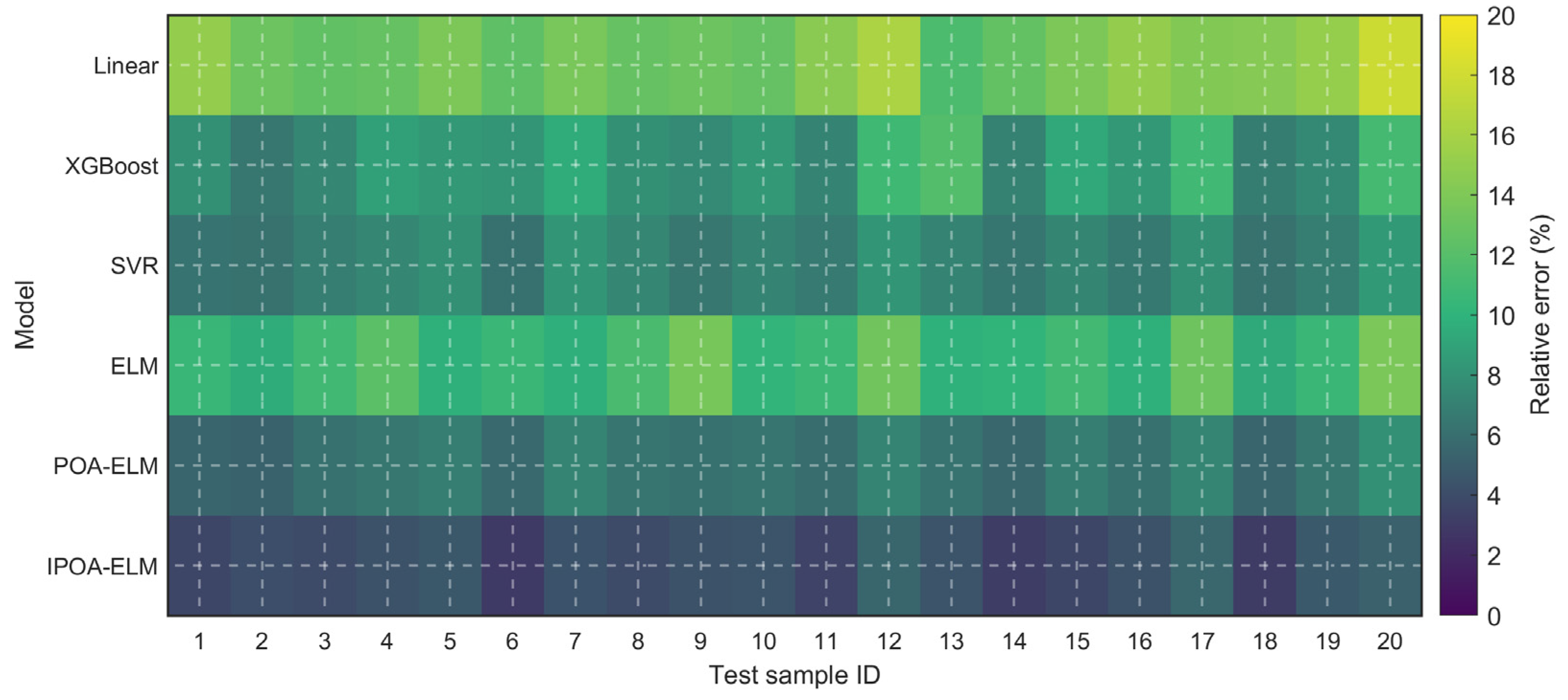
Figure 17 presents a combined comparison of measured and predicted slippage for the six models under the repeated k-fold evaluation; for clarity, one representative split is shown. Figure 18 reports the prediction relative error comparison across models and test samples. The results show that, relative to the ELM, both POA-ELM and IPOA-ELM align more closely with the measurements and yield smaller errors. Among the baseline models considered, SVR and XGBoost are competitive but remain below IPOA-ELM, whereas linear regression shows the largest errors. These findings indicate that the pelican optimization strategy effectively searches for better parameter settings and contributes to an improved prediction accuracy.
As shown in Figure 18, the per-sample relative error comparison clearly differentiates the performance of the six models. The proposed IPOA-ELM achieves the smallest errors across the majority of samples and maintains the highest accuracy, particularly on those with a large slippage. POA-ELM ranks as the second-best performer. Among the remaining baselines, SVR and XGBoost demonstrate a comparable performance, although their errors increase substantially on the most challenging samples. The traditional ELM performs below SVR and XGBoost but surpasses linear regression, which exhibits the largest errors for most samples. The superiority of IPOA-ELM stems from three key design innovations: a Halton sequence initialization for enhanced population diversity, an adaptive weight strategy for tuned search pressure, and Gaussian perturbations of pelican positions to balance global exploration and local refinement. Collectively, these mechanisms enable IPOA-ELM to better capture the underlying variation trend of slippage and thereby achieve a significant reduction in prediction error.
To make the error structure explicit, Figure 19 shows a predicted-versus-measured scatter for IPOA-ELM with the 45 ° reference line. Points lie close to the diagonal, with a slightly larger dispersion at a higher slippage. The metrics for this representative split, R 2 , MAE, and RMSE, are annotated on the plot, while the cross-validated aggregates are reported in Table 3.
Table 3 presents, under the repeated k-fold evaluation, a comparison of the evaluation metrics across different model algorithms. Compared with the other models, IPOA-ELM consistently achieves the lowest MAE, RMSE, and MAPE and the highest R 2 . POA-ELM comes next; SVR and XGBoost perform at a similar level, and ELM trails these but still outperforms linear regression. All four metrics consistently indicate that IPOA optimization significantly improves the performance of ELM. In conclusion, the proposed IPOA-ELM model can predict slippage more accurately. Moreover, slippage prediction effectively indicates the wear state of the traction sheave and provides a practical basis for forecasting and maintaining traction sheave wear faults in elevators.

4.4. Ablation Analysis of IPOA-ELM

To quantify the incremental benefit of each mechanism, we conduct an ablation analysis of IPOA-ELM that evaluates the incremental contribution of three key components: Halton sequence initialization, an adaptive weighting strategy, and Gaussian perturbation of pelican positions. This analysis measures how much each choice contributes to the performance gains observed in our dataset.
The ablation is configured so that only the targeted component is changed while all other settings are identical to the full model. Concretely, we construct three controlled variants by replacing Halton with random initialization, replacing adaptive weighting with a fixed weight, and removing the Gaussian perturbation. All settings follow the same data preprocessing and validation protocol as in Section 4.3 and are executed for thirty independent runs with a maximum of one hundred iterations, using fixed but distinct random seeds across runs to ensure reproducibility. Performance is summarized by MAE, RMSE, and R 2 . We further introduce the percentage %Improvement, a metric quantifying the relative reduction in RMSE. This metric quantifies the percentage reduction in error achieved by the full IPOA-ELM relative to each variant, where larger values indicate a greater error reduction. Its computation formula is as follows:
% I m p r o v e m e n t   =   100 × R M S E v a r i a n t R M S E I P O A E L M R M S E v a r i a n t
In Equation (35), R M S E v a r i a n t denotes the RMSE of the ablated variant (random initialization, fixed weight, or no Gaussian perturbation) and R M S E I P O A E L M denotes the RMSE of the full IPOA-ELM.
Table 4 summarizes the ablation results under the same data preprocessing and evaluation protocol. Relative to the full IPOA-ELM, all three variants deteriorate across MAE, RMSE, and R 2 . Replacing Halton with random initialization leads to a noticeably larger MAE and RMSE and a clear drop in R 2 , indicating that structured sampling at initialization helps stabilize the search and reduce prediction error. Fixing the weight instead of using adaptive weighting causes the most pronounced degradation, with errors increasing the most and R 2 decreasing the furthest. This result highlights adaptive weighting as the primary contributor among the three mechanisms. Removing Gaussian perturbation has the smallest yet still evident impact: errors increase moderately and R 2 decreases slightly, suggesting that the perturbation mainly improves local refinement and robustness rather than driving the bulk of the gains. Overall, IPOA-ELM attains the lowest MAE and RMSE and the highest R 2 among all settings, confirming that the three components act synergistically to improve prediction accuracy.
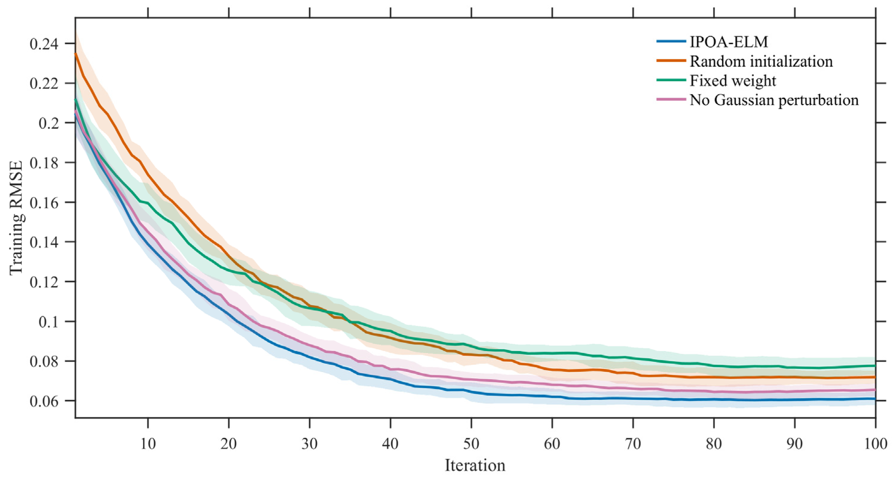
Figure 20 shows the training RMSE versus iterations for the full IPOA-ELM and three ablated variants. Each solid line is the mean over 30 runs; the translucent band denotes the mean plus and minus one standard deviation. The full IPOA-ELM drops fastest and settles at the lowest level, with the narrowest band, indicating a rapid and stable convergence. Removing Gaussian perturbation yields a curve slightly above the full model: the final level is close, but the band widens somewhat in the mid–late stage, suggesting a weaker local refinement. With random initialization instead of Halton, the curve starts higher, converges more slowly early on, and ends clearly above the full model, highlighting the benefit of a structured initialization. The fixed weight degrades the most: it has the slowest descent, highest plateau, and widest band, pointing to adaptive weighting as the major contributor. The bands shrink as iteration proceeds, and gains become small after about two-thirds of the budget. Overall, Halton aids early exploration, adaptive weighting balances global search and local exploitation, and Gaussian perturbation refines locally; together, they deliver a faster and more stable convergence for IPOA-ELM.

4.5. Robustness and Sensitivity of IPOA-ELM

To evaluate the stability of the IPOA–ELM under randomness and modest design choices, we conduct a robustness and sensitivity study that examines the effects of the hidden-layer size and the activation function. The analysis quantifies the performance variability under multiple random seeds and small hyperparameter changes.
The study is configured so that only the targeted factor is changed, while all other settings are kept identical to the baseline. Training and evaluation follow the same data preprocessing and validation protocol as in the previous subsections, namely 10 × 10 repeated cross-validation on the 82-sample dataset with independent random seeds. For robustness, the full procedure is repeated over multiple seeds, and the validation performance is summarized by the mean and standard deviation of RMSE. For sensitivity, one factor is varied at a time, while the others remain fixed to the baseline: the hidden size takes the values 8, 10, and 12; the activation function uses sigmoid, tanh, and ReLU. IPOA is fixed with a population size of 30 and 100 iterations and uses RMSE as the fitness.
Table 5 summarizes the robustness and sensitivity results under the same preprocessing and evaluation protocol as in Section 4.3 and Section 4.4. Here, the mean ± SD denotes the average validation RMSE over all folds, repeats, and random seeds, and SD is the sample standard deviation that quantifies the dispersion caused by data splits and seed randomness. Across configurations, the SD stays within a narrow band relative to the mean level, indicating a limited variability and good stability. The baseline with L   =   10 and sigmoid achieves the lowest average RMSE. Reducing the hidden size to L   =   8 increases both the mean error and SD, which is consistent with underfitting. Increasing it to L = 12 produces only a small change, suggesting that L   =   10 offers a balanced capacity for this dataset. Changing the activation from sigmoid to tanh yields a similar mean and SD, whereas ReLU shows a clearly larger mean error and variability, implying a lower stability with a small hidden layer. Overall, the small SDs and the consistent ranking across settings confirm that the model is insensitive to modest variations in L and activation, supporting the reliability of the earlier comparisons and ablations.
We further assess the input-level sensitivity of IPOA-ELM to the three key inputs: wear, load, and τ . In our data, T1 and T2 are the rope tensions on the tight and slack sides of the sheave. Although recorded as two channels, they describe the same traction state and vary in a strongly coupled manner. Using both as separate inputs would duplicate information and create collinearity with the load. Therefore, we replace T1 and T2 with a single, dimensionless indicator τ that captures their relative imbalance and is insensitive to a common scale change. The expression of τ is given in Equation (36):
τ   =   ln T 1 T 2
The sensitivity experiment follows exactly the same data, preprocessing, and validation setup as described above, namely 10 × 10 repeated k-fold cross-validation on the 82-sample dataset with a fixed grid of random seeds. In each fold, the model is trained on the original training split; on the corresponding validation split, we permute one input at a time, while keeping all other inputs and the trained model unchanged. This isolates the marginal influence of that input on the prediction. For reporting, we use a compact score defined as follows:
R M S E   =   R M S E ¯ p e r m R M S E ¯ b a s e
In Equation (37), R M S E ¯ b a s e denotes the fold-averaged validation RMSE without permutation, and R M S E ¯ p e r m denotes the fold-averaged validation RMSE when the selected input is permuted, and the averaging is taken over all folds and repeats.
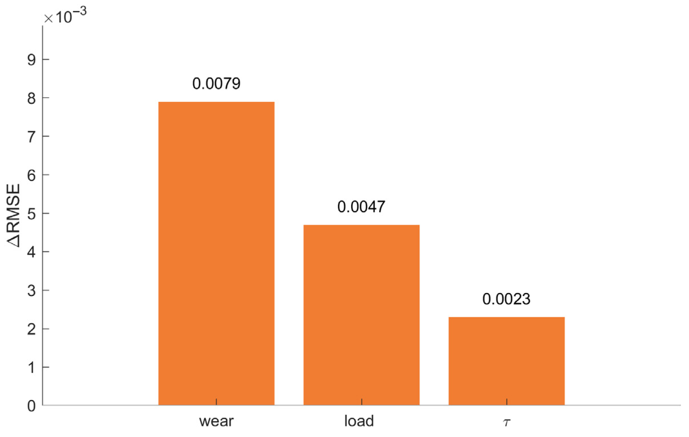
Figure 21 reports the permutation-based input sensitivity. Shuffling wear causes the largest degradation, followed by the load, while τ has the smallest effect. The absolute magnitudes indicate that no single input fully dominates the predictor, yet the ranking is clear. This ordering aligns with traction mechanics: wear directly alters the effective friction and contact geometry, thus impacting slippage the most; the load mainly changes the required traction level; and τ reflects the side-to-side balance and contributes less independent information once wear and load are given. Practically, the results suggest prioritizing accurate sensing and calibration of wear, followed by load, with τ being informative but secondary in this setting.

5. Conclusions

This paper first delves into the factors influencing the constant-speed, acceleration, and deceleration processes through a mechanistic analysis. On this basis, a machine learning approach is employed utilizing the Improved Pelican Optimization Algorithm (IPOA) to optimize the Extreme Learning Machine (ELM) model for slippage prediction, significantly improving prediction accuracy. By accurately predicting the slippage, the model provides a theoretical foundation for elevator health monitoring, offering significant implications and practical value for elevator fault prediction.
(1)
Through the study of the slippage mechanism between the elevator traction sheave and the wire rope, it is found that the equivalent friction coefficient and the rope’s wrap angle on the sheave groove are the key factors determining the traction capacity. For a semicircular groove with a notch, the traction capacity ceases to change once the wear depth reaches a certain level. During constant-speed operation and acceleration/deceleration, the slippage mainly depends on the material properties of the wire rope, the contact length, the load difference, and the wear of the groove. These analyses provide theoretical support for the prediction of elevator slippage. Practically, within the tested operating envelope, wear has the largest marginal impact on slippage. Load is secondary, and the tension ratio τ is least influential. Accordingly, maintenance should prioritize wear inspection and calibration, followed by load balancing.
(2)
The IPOA is improved by introducing the Halton sequence, Gaussian perturbation, and a nonlinear inertia weight factor to optimize the initial weights and biases of the ELM. Comparative experiments indicate that, relative to traditional ELM and POA-ELM, as well as SVR, XGBoost, and a physics-informed linear baseline, IPOA-ELM attains a lower MAE, RMSE, and MAPE and a higher R 2 , with a faster and smoother convergence; ablation tests attribute the gains to the combined effect of Halton initialization, the bounded sine-based adaptive weight, and Gaussian perturbation, while robustness checks show a small dispersion under repeated runs and a stable performance under moderate hyperparameter changes. Unlike POA variants that mainly target local-extrema handling, this design enlarges early exploration and enforces a controlled late-stage contraction, yielding consistent advantages in accuracy and stability.
(3)
The observed relationship between groove wear and slippage provides a basis for real-time failure risk assessment. By accurately predicting abnormal slippage trends, this method enables the timely identification of traction sheave degradation, supporting the development of predictive maintenance schedules. This contributes to a broader engineering objective of preventing structural or operational failures in elevator systems.
This study used data from a single traction system under a fixed configuration; therefore, the findings primarily reflect this operating envelope and should not be directly extrapolated to other sheave diameters, groove geometries, rope constructions, speeds, or control systems. For application to other elevators, we recommend collecting a small calibration set under the target configuration, re-normalizing variables, retraining the ELM using the same repeated k-fold protocol, and verifying the performance on an external bench or in-field run. Environmental factors and maintenance conditions that affect friction were not varied here and may require additional calibration.
For practical deployment, the proposed slippage predictor can be integrated into elevator monitoring and maintenance systems. A lightweight inference module on the controller or edge gateway ingests traction sheave encoder signals, rope-end tensions, and command streams, produces per-trip and daily slip-risk scores, and triggers graded alerts with auto-generated work orders when thresholds are exceeded or sustained upward trends are detected. The alerts and follow-up actions are written back to the asset record and linked with condition-based maintenance planning to form a traceable closed loop. Guided by the input-level sensitivity results, wear, load, and the tension ratio should be treated as priority indicators, and coupling the predictor with a digital twin or life-assessment model can enable earlier warnings and a more rational allocation of spare parts and maintenance resources.
Future work may focus on integrating the proposed model into elevator control systems and expanding its application to other rope-based lifting mechanisms. The approach also offers potential value in enhancing structural integrity monitoring in other transportation or mechanical domains where frictional failure is critical.

Author Contributions

Conceptualization, Y.W., J.C. and Q.W.; methodology, Y.W. and P.Y.; software, Y.W.; validation, Y.W., Q.W., P.Y. and J.C.; formal analysis, Y.W., P.Y. and J.C.; investigation, Y.W. and J.C.; resources, P.Y. and J.C.; data curation, Y.W.; writing—original draft preparation, Y.W.; writing—review and editing, J.C.; visualization, Q.W.; supervision, P.Y. and J.C.; project administration, P.Y.; funding acquisition, P.Y. and J.C. All authors have read and agreed to the published version of the manuscript.

Funding

This research was funded by Science and Technology Program of the State Administration for Market Regulation, grant number 2024MK054.

Institutional Review Board Statement

Not applicable.

Informed Consent Statement

Not applicable.

Data Availability Statement

The data presented in this study are openly available in Zenodo at https://doi.org/10.5281/zenodo.17320872.

Acknowledgments

The authors would like to thank the reviewers for their insightful comments and constructive suggestions.

Conflicts of Interest

The authors declare no conflicts of interest.

Abbreviations

The following abbreviations are used in this manuscript:
ELMExtreme Learning Machine
POAPelican Optimization Algorithm
IPOAImproved Pelican Optimization Algorithm
SVRSupport Vector Regression
XGBoostExtreme Gradient Boosting
RMSERoot Mean Square Error
MAEMean Absolute Error
R2Coefficient of Determination
MAPEMean Absolute Percentage Error
SDStandard Deviation

References

  1. Zhen, Q.; Wu, Y.; Cong, J.; Lyu, S.-K. Mechanism Design and Experimental Verification of Novel Automatic Balance Equipment for a Rope-Type Elevator. Machines 2022, 10, 1180. [Google Scholar] [CrossRef]
  2. Zhang, J.; Wang, D.; Zhang, D.; Ge, S.; Araújo, J.A. Dynamic Contact and Slip Characteristics of Bent Hoisting Rope in Coal Mine. J. Braz. Soc. Mech. Sci. Eng. 2018, 40, 120. [Google Scholar] [CrossRef]
  3. Nakazawa, D.; Watanabe, S.; Fukui, D.; Fujii, A.; Miyakawa, K. Elevator Rope Tension Analysis with Uneven Groove Wear of Sheave. J. Phys. Conf. Ser. 2018, 1048, 12006. [Google Scholar] [CrossRef]
  4. Zheng, Q.; Wang, D.; Zhang, K.; Ma, J.; Ding, G.; Zhang, Y.; Yuan, Z. A Parametric Study on the Fatigue Life of Elevator Brake Wheels under Multi-Field Coupling Effects. Eng. Fail. Anal. 2025, 167, 109061. [Google Scholar] [CrossRef]
  5. Chen, J.; Jing, L.; Hong, T.; Liu, H.; Glowacz, A. Research on a Sliding Detection Method for an Elevator Traction Wheel Based on Machine Vision. Symmetry 2020, 12, 1158. [Google Scholar] [CrossRef]
  6. Ma, X.; Pan, Y.; Shi, X. Experimental Investigation of Friction and Slip at the Traction Interface of Rope and Sheave. J. Appl. Mech. 2018, 85, 11006. [Google Scholar] [CrossRef]
  7. Guo, Y.; Zhang, D.; Zhang, X.; Wang, D.; Wang, S. A New Transmission Theory of “Global Dynamic Wrap Angle” for Friction Hoist Combining Suspended and Wrapped Wire Rope. Appl. Sci. 2020, 10, 1305. [Google Scholar] [CrossRef]
  8. Samal, S.; Dash, R. A Hybrid Fruit Fly ELM Framework for Stock Index Price Movement Prediction. In Proceedings of the 2021 International Conference in Advances in Power, Signal, and Information Technology (APSIT), Bhubaneswar, India, 8–10 October 2021; pp. 1–5. [Google Scholar]
  9. Li, L.; Liu, K.; Wang, L.; Sun, L.; Zhang, Z.; Guo, H. Fault Diagnosis of Balancing Machine Based on ISSA-ELM. Comput. Intell. Neurosci. 2022, 2022, 4981022. [Google Scholar] [CrossRef] [PubMed]
  10. Shao, H.; Jiang, H.; Li, X.; Wu, S. Intelligent Fault Diagnosis of Rolling Bearing Using Deep Wavelet Auto-Encoder with Extreme Learning Machine. Knowl.-Based Syst. 2018, 140, 1–14. [Google Scholar] [CrossRef]
  11. Yang, D.; Yang, K. Multi-Step Prediction of Strong Earthquake Ground Motions and Seismic Responses of SDOF Systems Based on EMD-ELM Method. Soil Dyn. Earthq. Eng. 2016, 85, 117–129. [Google Scholar] [CrossRef]
  12. Yaseen, Z.M.; Deo, R.C.; Hilal, A.; Abd, A.M.; Bueno, L.C.; Salcedo-Sanz, S.; Nehdi, M.L. Predicting Compressive Strength of Lightweight Foamed Concrete Using Extreme Learning Machine Model. Adv. Eng. Softw. 2018, 115, 112–125. [Google Scholar] [CrossRef]
  13. Kaloop, M.R.; Kumar, D.; Samui, P.; Gabr, A.R.; Hu, J.W.; Jin, X.; Roy, B. Particle Swarm Optimization Algorithm-Extreme Learning Machine (PSO-ELM) Model for Predicting Resilient Modulus of Stabilized Aggregate Bases. Appl. Sci. 2019, 9, 3221. [Google Scholar] [CrossRef]
  14. Ge, D.; Zhang, Z.; Kong, X.; Wan, Z. Extreme Learning Machine Using Bat Optimization Algorithm for Estimating State of Health of Lithium-Ion Batteries. Appl. Sci. 2022, 12, 1398. [Google Scholar] [CrossRef]
  15. Xiong, J.; Peng, T.; Tao, Z.; Zhang, C.; Song, S.; Nazir, M.S. A Dual-Scale Deep Learning Model Based on ELM-BiLSTM and Improved Reptile Search Algorithm for Wind Power Prediction. Energy 2023, 266, 126419. [Google Scholar] [CrossRef]
  16. Huang, G.; Huang, G.-B.; Song, S.; You, K. Trends in Extreme Learning Machines: A Review. Neural Netw. 2015, 61, 32–48. [Google Scholar] [CrossRef] [PubMed]
  17. Ding, S.; Zhao, H.; Zhang, Y.; Xu, X.; Nie, R. Extreme Learning Machine: Algorithm, Theory and Applications. Artif. Intell. Rev. 2015, 44, 103–115. [Google Scholar] [CrossRef]
  18. Li, D.; Li, S.; Zhang, S.; Sun, J.; Wang, L.; Wang, K. Aging State Prediction for Supercapacitors Based on Heuristic Kalman Filter Optimization Extreme Learning Machine. Energy 2022, 250, 123773. [Google Scholar] [CrossRef]
  19. Wang, J.; Lu, S.; Wang, S.-H.; Zhang, Y.-D. A Review on Extreme Learning Machine. Multimed. Tools Appl. 2022, 81, 41611–41660. [Google Scholar] [CrossRef]
  20. Trojovsky, P.; Dehghani, M. Pelican Optimization Algorithm: A Novel Nature-Inspired Algorithm for Engineering Applications. Sensors 2022, 22, 855. [Google Scholar] [CrossRef]
  21. Krömer, P.; Platoš, J.; Snášel, V. Differential Evolution for the Optimization of Low-Discrepancy Generalized Halton Sequences. Swarm Evol. Comput. 2020, 54, 100649. [Google Scholar] [CrossRef]
  22. Qiao, L.; He, N.; Cui, Y.; Zhu, J.; Xiao, K. Reservoir Porosity Prediction Based on BiLSTM-AM Optimized by Improved Pelican Optimization Algorithm. Energies 2024, 17, 1479. [Google Scholar] [CrossRef]
  23. Lv, L.; Zhao, J. The Firefly Algorithm with Gaussian Disturbance and Local Search. J. Signal Process. Syst. 2018, 90, 1123–1131. [Google Scholar] [CrossRef]
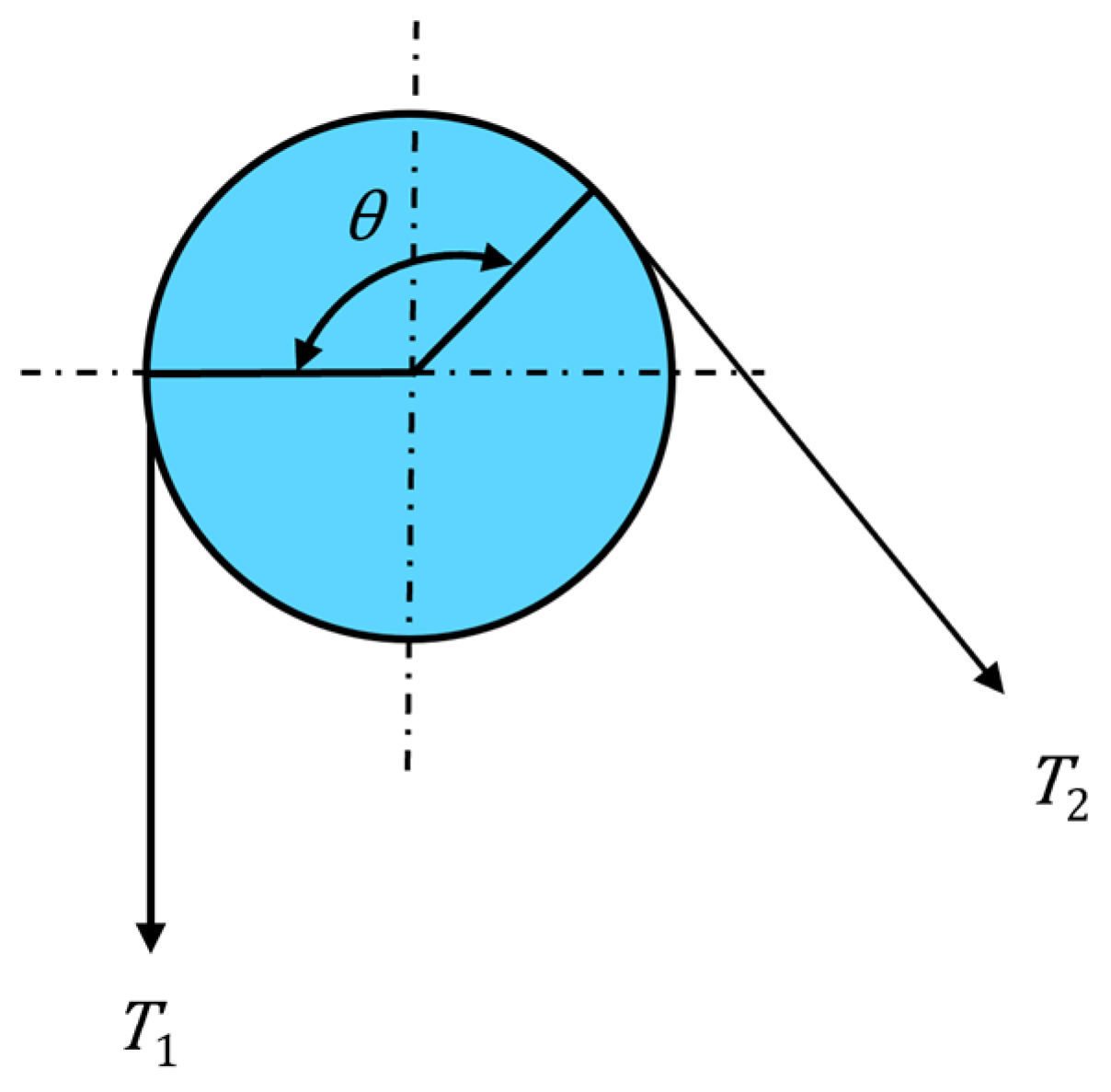
Figure 1. Diagram of wire rope contact with the traction sheave.
Applsci 15 11802 g001
Figure 2. Notched semicircular groove.
Applsci 15 11802 g002
Figure 3. Wear groove angle analysis diagram.
Applsci 15 11802 g003
Figure 4. Analysis of the variation in the notch angle.
Applsci 15 11802 g004
Figure 5. Graph of the relationship between groove angle and wear depth.
Applsci 15 11802 g005
Figure 6. Wear depth–traction capacity with sensitivity analysis.
Applsci 15 11802 g006
Figure 7. Slippage between the traction sheave and the steel wire rope.
Applsci 15 11802 g007
Figure 8. Heavy-load downward braking process.
Applsci 15 11802 g008
Figure 9. Force analysis of the traction sheave.
Applsci 15 11802 g009
Figure 10. The force analysis at the contact point between the wire rope and the traction sheave.
Applsci 15 11802 g010
Figure 11. Principle of the Extreme Learning Machine.
Applsci 15 11802 g011
Figure 12. Random initialization of population distribution.
Applsci 15 11802 g012
Figure 13. Halton sequence initialization of population.
Applsci 15 11802 g013
Figure 14. Extreme Learning Machine optimized by the Improved Pelican Optimization Algorithm.
Applsci 15 11802 g014
Figure 15. On-site data acquisition device.
Applsci 15 11802 g015
Figure 16. IPOA optimization iteration process.
Applsci 15 11802 g016
Figure 17. Prediction results of different models.
Applsci 15 11802 g017
Figure 18. Per-sample relative error comparison.
Applsci 15 11802 g018
Figure 19. Predicted versus measured slippage for IPOA-ELM.
Applsci 15 11802 g019
Figure 20. Convergence of IPOA-ELM and ablated variants in training RMSE.
Applsci 15 11802 g020
Figure 21. Input level sensitivity comparison.
Applsci 15 11802 g021
Table 1. Basic parameters of the test elevator.
ParameterValueParameterValue
Number of floors2Number of ropes5
Floor height3.5 mAcceleration0.3 m/s2
Elastic modulus 2 × 10 11   P a Number of grooves5
Rated load1000 kgRated speed0.6 m/s
Traction ratio1:1Traction sheave diameter400 mm
Groove typeSemicircular grooveWire rope diameter10 mm
Balance coefficient0.45
Table 2. Partial slippage data obtained from the experiment.
Wear Amount
(mm)
Load Weight
(%)
T1
(N)
T2
(N)
Slippage
(mm)
00148318930.10
0100264818610.17
0125289119110.32
0.50142819050.71
0.5100261818320.88
0.5125292419211.13
10147918870.6
1100258818020.74
1125294919110.99
20144918820.72
2100264118320.9
2125292019201.22
40145219010.59
4100266218590.73
4125304920180.94
50145918950.69
5100266019010.76
5125294120201.31
60148819210.78
6100257518250.91
7125147519030.74
7.30149219120.71
Table 3. Comparison of evaluation metrics for different model algorithms.
ModelMAERMSE R 2 MAPE (%)
Linear0.11200.14040.710112.0
ELM0.10150.12720.761910.9
XGBoost0.07340.09200.87587.9
SVR0.06980.08750.88747.5
POA-ELM0.06690.08380.89617.2
IPOA-ELM0.04790.06030.94715.1
Table 4. Comparison of evaluation metrics for IPOA-ELM and its ablated variants.
SettingMAERMSE R 2 %Improvement
IPOA-ELM0.04870.06100.9445
Random initialization0.05740.07190.922815.2%
Fixed weight0.06190.07760.910121.4%
No Gaussian perturbation0.05230.06550.93606.9%
Table 5. Sensitivity of IPOA-ELM to hidden size and activation.
SettingLActivationValidation RMSE
(Mean ± SD)
Baseline10Sigmoid0.057 ± 0.004
Vary L down8Sigmoid0.061 ± 0.005
Vary L up12Sigmoid0.060 ± 0.005
Change activation10Tanh0.059 ± 0.004
Change activation10ReLU0.063 ± 0.006
Disclaimer/Publisher’s Note: The statements, opinions and data contained in all publications are solely those of the individual author(s) and contributor(s) and not of MDPI and/or the editor(s). MDPI and/or the editor(s) disclaim responsibility for any injury to people or property resulting from any ideas, methods, instructions or products referred to in the content.