Article

Advancing Machine Learning-Based Streamflow Prediction Through Event Greedy Selection, Asymmetric Loss Function, and Rainfall Forecasting Uncertainty

1
Department of Mechanical Engineering, Iowa Technology Institute, University of Iowa, Iowa City, IA 52242, USA
2
Turkish Water Institute, Istanbul 34696, Türkiye
3
Department of Civil Engineering, University of Manitoba, Winnipeg, MB R3T 5V6, Canada
*
Authors to whom correspondence should be addressed.
Appl. Sci. 2025, 15(21), 11656; https://doi.org/10.3390/app152111656
Submission received: 12 October 2025 / Revised: 27 October 2025 / Accepted: 29 October 2025 / Published: 31 October 2025
(This article belongs to the Topic Data Science and Intelligent Management)

Abstract

This paper advances machine learning (ML)-based streamflow prediction by strategically selecting rainfall events, introducing a new loss function, and addressing rainfall forecast uncertainties. Focusing on the Iowa River Basin, we applied the stochastic storm transposition (SST) method to create realistic rainfall events, which were input into a hydrological model to generate corresponding streamflow data for training and testing deterministic and probabilistic ML models. Long short-term memory (LSTM) networks were employed to predict streamflow up to 12 h ahead. An active learning approach was used to identify the most informative rainfall events, reducing data generation effort. Additionally, we introduced a novel asymmetric peak loss function to improve peak streamflow prediction accuracy. Incorporating rainfall forecast uncertainties, our probabilistic LSTM model provided uncertainty quantification for streamflow predictions. Performance evaluation using different metrics improved the accuracy and reliability of our models. These contributions enhance flood forecasting and decision-making while significantly reducing computational time and costs.

1. Introduction

Streamflow forecasting is fundamental for effective decision-making in hydrology and water resource management, impacting flood mitigation strategies, watershed conservation, water supply management, hydropower generation, agricultural development, reservoir management, and various aspects of integrated water resource management. Nonetheless, the intricate and ever-changing nature of hydrological systems, often exhibiting nonlinear behaviors and variability, poses a continuous challenge in achieving precise streamflow predictions [1,2,3]. Various models, both process-based and data-driven, have been developed to tackle this challenge, each with its advantages and limitations [4].
Process-based models, rooted in the principles of hydrology and meteorology, employ differential equations to describe transport mechanisms in the surface and subsurface of a watershed [5,6,7]. These models have the advantage of modeling complex physical interactions, including water exchanges with the atmosphere and the movement of water in rivers and lakes [8]. However, they require extensive parameterization, high-quality input data, and significant computational resources, making them complex and sometimes impractical for large-scale or real-time applications. On the other hand, data-driven models capture statistical dependencies between explanatory inputs and response outputs, bypassing the need for explicit governing equations of the system [3,9]. These models are computationally efficient, adaptable to different conditions, and capable of capturing nonlinear relationships that may be oversimplified in process-based approaches. However, they may suffer from overfitting, data quality issues, and a lack of physical interpretability.
Specifically, the advent of machine learning (ML) and artificial intelligence (AI) has revolutionized the field of hydrology, particularly in streamflow forecasting, by offering new possibilities through enhanced computational capabilities and innovative algorithms. Traditional ML techniques, such as support vector machines (SVMs) and linear regression, have been employed in streamflow forecasting, achieving varying degrees of success [10,11]. However, recent breakthroughs in deep learning (DL), particularly the development of long short-term memory (LSTM) networks—a subset of recurrent neural networks (RNNs)—have shown great promise in capturing the temporal dependencies and complex patterns inherent in hydrological data.
Building on these advances, this study employs an LSTM-based architecture for streamflow forecasting. We acknowledge that the gated recurrent unit (GRU) offers a simpler architecture with fewer parameters, and Transformer-based models have shown strong performance in recent sequence modeling applications. However, compared to LSTMs, GRUs are less effective on complex tasks, while Transformers require substantially higher computational resources [12,13].
Many studies have shown that LSTM models often perform better than both traditional process-based and ML models in predicting streamflow [14,15,16,17,18,19,20,21,22]. For instance, Kratzert et al. [14] successfully employed an LSTM model for daily runoff prediction by incorporating meteorological data as input, demonstrating that these models outperformed process-based models in certain scenarios. Xiang et al. [15] proposed a sequence-to-sequence (seq2seq) model and demonstrated that this model surpasses traditional ML methods like linear regression, lasso regression, and ridge regression in terms of predictive accuracy and various other performance measures.
Hunt et al. [19] employed an LSTM model to predict streamflow at 10 river gauging stations across various climatic regions of the western United States, training it with meteorological and hydrological data. Their findings indicate that employing LSTM for medium-range streamflow forecasting outperforms traditional process-based models. Moreover, research conducted by Arsenault et al. [20] demonstrated that LSTM models exceeded the performance of traditional hydrological models in comprehensive evaluations across over 148 North American basins. Chen et al. [21] conducted a study employing a hybrid approach that integrated the soil water assessment tool (SWAT) with LSTM in ungauged and poorly gauged watersheds. They used SWAT to produce an extended data series of watershed processes, which, along with climatic data, served as inputs for the LSTM model. Their results demonstrate that this integration significantly improved the reliability and accuracy of streamflow simulations, outperforming the default SWAT simulations in these challenging watershed conditions. Moreover, Tursun et al. [22] performed streamflow analyses in 40 catchment areas within the Yellow River Basin, revealing that LSTM-based models hold considerable promise for accurately modeling river flow in arid regions affected by human interventions. These studies further affirm the robust capabilities of LSTM networks in challenging hydrological applications.
Despite all the advancements, significant challenges persist in streamflow forecasting using ML/DL models. Developing a robust model generally requires a substantial number of data samples. Furthermore, ML models that rely on traditional loss functions struggle to accurately predict peak streamflow events [14], which are usually driven by complex interactions among various factors, such as extreme weather conditions, rapid snow melt, and land use changes. These models often fail to capture the complexities involved, posing significant challenges in hydrological contexts where precise prediction of peak values is critical for effective flood risk mitigation, emergency responses, and water resource management.
Another critical limitation of these models is their inability to account for the uncertainties inherent in hydrological variables (e.g., rainfall) [23]. They offer point estimates of streamflow values that overlook these uncertainties or errors and fail to convey the associated uncertainty in predictions, potentially leading to less reliable streamflow forecasts [24]. This uncertainty is often expressed using prediction intervals or probabilistic distributions. Significant research in hydrology has focused on developing methods to quantify and represent such uncertainties within conventional modeling approaches [25,26]. A comparable level of dedication is needed to adapt these methodologies for DL models like LSTM. A variety of methods exist to assess prediction uncertainty. Most rely on enhancing a deterministic model with an additional uncertainty quantification component. Among these, ensemble-based modeling is particularly common, where outputs from multiple ensemble members are combined—using equal or weighted averaging—to approximate the probability distribution of the predicted variable [27,28]. Other commonly employed approaches encompass pre-processing and post-processing methods, including those grounded in Bayesian techniques and quantile regression methods [29,30,31].
To address these challenges, our study aims to introduce several innovative approaches to enhance the accuracy and reliability of streamflow predictions. Given the complexity of hydrological processes and the variability of storm events, traditional observation-based datasets may not always provide sufficient coverage for robust model evaluation. Therefore, after model calibration, we used datasets generated by process-based models instead of direct observations as they efficiently cover a broader range of storm event scenarios compared to USGS observations. This approach ensured that our models were tested under diverse conditions, including extreme events that might be underrepresented in observational records. Additionally, process-based models allowed for a more controlled and systematic demonstration of the proposed approaches, facilitating a comprehensive assessment of their performance and generalizability.
Firstly, to identify the most informative rainfall events and reduce the computational cost and time associated with hydrological simulations for data generation, we employed an active learning (AL) technique. While our previous study [32] preliminarily investigated the effect of training set size on ML model performance, it relied on randomly selecting storm events to generate training sets of varying sizes. The AL-based selection strategy used in this study advances our previous work, demonstrating a clear advantage over the random selection of rainfall events in our experiments.
Second, we proposed a novel asymmetric loss function designed to capture peak streamflow events more accurately. This approach improved the model’s ability to predict high-flow values, addressing a critical aspect of hydrological forecasting where symmetric loss functions might fall short. Compared to the pinball loss (PL) function [30], an available asymmetric loss function, the developed loss function yielded better performance from the ML predictive model.
Finally, we developed a probabilistic LSTM (PLSTM) model that integrates rainfall forecast uncertainties, providing a range of probable streamflow outcomes rather than a single deterministic output. Differing from other studies that used ensemble methods [27,28], Bayesian techniques [29,31], and quantile regression [30], our PLSTM probabilistic modeling technique uses negative log-likelihood (NLL) to quantify uncertainty directly during model training. Using this technique, the model estimates prediction uncertainty without the need for ensemble methods or Bayesian techniques, offering an efficient yet reliable solution for streamflow predictions. Unlike most existing studies, which assume deterministic and accurate rainfall forecasts, this approach advances by incorporating rainfall forecast errors into the training data, capturing both the expected value and the associated uncertainty of streamflow predictions. This methodology aligns with and extends the current state of the art by applying probabilistic techniques within DL frameworks to address uncertainty in hydrological modeling.
Through these approaches, our goal is to redefine the benchmarks for streamflow forecasting by integrating advanced ML methods with deep hydrological understanding, thereby enhancing the precision and practical applicability of predictions for flood early warning systems, reservoir operation, and other strategic planning.
The remainder of this paper is organized as follows: Section 2 presents a description of the study area, outlines the process-based modeling framework, and details the calibration procedure. Section 3 describes the data generation, including rainfall event selection and dataset creation. Section 4 introduces the LSTM-based encoder–decoder model for deterministic streamflow prediction and demonstrates the advantage of greedy rainfall event selection. Section 5 presents a novel loss function designed to emphasize peak streamflow prediction. Section 6 incorporates rainfall forecasting errors into the training data and develops a probabilistic LSTM model for quantifying uncertainty in streamflow predictions. Finally, Section 7 concludes the paper.

2. Hydrological Model

2.1. Iowa River Basin

The focus area of this study encompasses the Iowa River Basin and its internal river network. Located in the central and eastern regions of Iowa, the Iowa River Basin drains an area of roughly 11,140 km 2 before reaching Columbus Junction. The basin is continuously monitored by more than 20 USGS gauging stations. Over the last twenty years, this region has experienced a series of recurrent flood events, resulting in significant damage to individuals, agricultural activities, and infrastructure across different scales. In 2008, a substantial flood event impacted 86 counties in Iowa, leading to its designation as a federal disaster zone. This event incurred costs totaling USD 11 billion in damages and affected over 41,000 individuals [33]. Figure 1 depicts the Iowa River Basin along with the locations of the USGS stations.
A part of the Iowa River is regulated by the Coralville Dam within this basin, as indicated by its position in Figure 1. The dam has been operational since 1959, and it is an earthfill dam spanning 426 m in length and standing 30 m tall. It creates the Coralville Reservoir on the Iowa River, situated 134 km upstream from its merging point with the Mississippi River and 8 km above Iowa City, IA. The main objective of this dam is to manage flood risks for regions along the Iowa River [34]. Above the dam, the Iowa River receives drainage from approximately 8068 km 2 , primarily consisting of agricultural lands. Additionally, about 3052 km 2 of drainage areas from the dam location to Columbus Junction flow downstream, eventually reaching the Mississippi River.

2.2. Semi-Distributed HEC-HMS Hydrological Model

To simulate the rainfall–runoff transformation process in the basin, the semi-distributed event-based hydrologic modeling system (HEC-HMS) was employed [35]. Specifically, after delineating the Iowa River Basin using a 30-meter-resolution digital elevation model (DEM) and identifying the river network, rainfall data as a time series for each subbasin was fed into the model. The rainfall loss through infiltration was estimated using the Soil Conservation Service-Curve Number (SCS-CN) method [35]. This method calculates the direct runoff depth, denoted as P e (mm)
P e = ( P I a ) 2 P I a + S
where P is the accumulated rainfall depth (mm), and S represents the potential maximum retention (mm), linked to curve number (CN). Additionally, I a denotes the initial abstraction (mm), which can be expressed as a function of S ( I a = 0.2 S ). The model inputs consist of I a , CN, and the percentage of impervious area (no loss calculations are conducted on the impervious areas) [35].
The standard Clark Unit Hydrograph method [35] was employed to simulate runoff routing within the basin. The parameters essential for this transformation include the time of concentration, defined as the time needed for excess rainfall to travel from the most hydraulically remote point in the basin to the outlet, and the storage coefficient, which represents the attenuation resulting from storage effects throughout a basin. These parameters were calculated based on the physical properties of the basin. The recession method was also employed for determining the baseflow [35]. The parameters required for the recession method include the initial baseflow at the start of the simulation and the recession constant. The initial baseflow was specified using the discharge rate method, following the guidelines outlined in the HEC-HMS technical manual [35]. The recession constant was initially selected within the recommended range of 0.3–0.8 for each subbasin and was subsequently refined through model calibration to improve agreement with observed hydrographs.
Finally, the simulation of flood routing along natural channels was conducted using the Muskingum routing method [35]. This method uses the principle of conservation of mass to estimate the outflow hydrograph from the channel. Muskingum routing requires several parameters, including the Muskingum K parameter (representing travel time through a reach), the dimensionless coefficient X (ranging from 0.0 to 0.5, 0 for maximum attenuation and 0.5 for no attenuation), and the number of sub-reaches that can be calculated by dividing the Muskingum K parameter by the simulation time step.
The simulation of routing from a reservoir is also integrated within the HEC-HMS model through different methods: outflow structure routing, outflow curve routing, and specified release routing [35]. We utilized the outflow structure routing method. A dam reservoir was defined by the elevation–storage curve and by a specification of an outlet. The outlet was defined by an inlet control with the discharge flowing out from the outlet when it is submerged, expressed as follows:
Q c = A c C d 2 g h
(where Q c is the outlet discharge (cms), A c represents the cross-sectional area of the outlet (m2), which is circular with a diameter of 7 m in Coralville Dam [34], C d denotes the discharge coefficient (equal to 0.8), g is the gravitational acceleration (9.81 m/s2), and h stands for the total water head (m).

2.3. Model Calibration

The HEC-HMS model was calibrated using a single flood event that took place from 8 to 28 June 2008 within the study area. Hourly temporal resolution data from this event were utilized in the calibration process. This calibration involved providing streamflow observations obtained from USGS streamflow data at the outlet of each subbasin, corresponding to the locations of the stream gauges defined in Figure 1. For model calibration downstream of the Coralville Dam, streamflow data observed at a USGS station immediately downstream of the dam were used. This data included releases from the Coralville Dam, which were used as boundary conditions for the model in the downstream subbasin. In the calibration of the model, we considered statistical metrics such as the Nash–Sutcliffe efficiency (NSE), root mean squared error ratio (RSR), and percent bias (PBIAS), as formulated below.
NSE = 1 i = 1 N ( O i y i ) 2 i = 1 N ( O i O ¯ ) 2
RSR = RMSE σ o = i = 1 N ( O i y i ) 2 i = 1 N ( O i O ¯ ) 2
PBIAS = i = 1 N ( O i y i ) × 100 i = 1 N O i
where O i is the observed value, y i is the simulated value, O ¯ is the average of observed values, σ o is the standard deviation of observed values, and N is the total number of observations.
In general, model simulation can be judged as satisfactory if NSE > 0.50, RSR ≤ 0.70, and PBIAS is within ±25% for streamflow [36]. Table 1 presents the statistical metrics obtained after calibrating the HEC-HMS model for the study area. A peak streamflow is defined as a normalized streamflow value greater than 0.45, where the normalized streamflow is calculated by dividing the observed streamflow by the maximum streamflow recorded during the event. To further validate the calibrated model, we applied it to a distinct event that occurred from 26 April to 14 May 2013 within the studied basin. Table 2 presents the calculated metrics, all of which fall within these acceptable ranges. Therefore, the model was well-configured and ready for simulating flood hydrographs.

3. Data Generation

3.1. Rainfall Event Generation

The stochastic storm transposition (SST) method [32] was utilized to create synthetic rainfall events that realistically represent the spatial and temporal variability in the study region. This approach extends the duration of extreme rainfall scenarios at a given location by transposing rainfall patterns from nearby areas exhibiting comparable extreme rainfall behavior.
The rainfall data for this study was generated using RainyDay [37], an open-source Python-based software available from the Hydroclimate Extremes Group (https://github.com/HydroclimateExtremesGroup/RainyDay, accessed on 20 September 2025). RainyDay integrates gridded rainfall data with the SST framework. The RainyDay implementation of the SST approach involves five primary stages: (1) define a transposition domain ( A D ) that encompasses the target area ( A w ). It is recommended that the A D be at least four times larger than A w [37]; (2) identify m temporally independent storms within A D using n years of rainfall records. These storms are extracted based on accumulated rainfall over a duration t, with spatial characteristics (size, shape, and orientation) aligned to A D to construct a “storm catalog”; (3) specify the number of storms per year, k, determined either via a Poisson distribution or an empirical distribution; (4) randomly sample k storms from the catalog; and (5) repeat steps 3 and 4 for a designated number of simulation years, T max , to produce T max years of t-hour synthetic annual rainfall maxima for A w .
For the present study, gridded Stage IV rainfall data spanning from 2002 to 2021, featuring a temporal resolution of 1 h and a spatial resolution of 4 km, were utilized to construct a storm catalog for spatiotemporal resampling. The A D covered 95.36–90.11° W and 40.23–44.73° N. This extent is approximately four times larger than the study area, consistent with the recommendation. The storm catalog included the 200 highest-intensity rainfall events identified within the defined domain, which was considered sufficient to represent the basin’s hydrometeorological variability while maintaining computational efficiency for subsequent simulations. These extreme events were selected based on 72-h rainfall accumulations evaluated over regions matching the Iowa River Basin in both size and shape. The random variable k was modeled using a Poisson distribution with a rate parameter ( λ = 10 ), calculated as the ratio of the total number of cataloged events to the number of years in the rainfall record.
In this study, the Iowa River Basin was divided into five subbasins before the Lone Tree, as illustrated in Figure 1. These subbasins were selected based on the presence of USGS gauge stations along the river’s mainstream and the availability of data at those stations. Subsequently, the average rainfall time series for each subbasin was determined using zonal averaging.

3.2. Greedy Event Selection

While using the SST facilitates the generation of a wide range of rainfall events, enhancing both the diversity and duration of extreme precipitation, obtaining the corresponding streamflow responses necessitates hydrologic simulations. These simulations are computationally intensive and time-consuming, rendering the large-scale generation of rainfall–runoff events impractical. Moreover, random selection of rainfall events proves inefficient, often resulting in redundant or uninformative events to generate data that contribute minimally to model improvement. To address this limitation, active learning (AL) for regression offers a promising solution by reducing the number of required simulations through the strategic selection of the most informative rainfall events [38].
This paper focuses on pool-based AL [39], in which a pool of 200 rainfall events randomly generated using RainyDay is considered. The objective is to select a subset of these events for hydrological simulations to generate data, aiming to train an LSTM model that can provide highly accurate streamflow estimates for the remaining events. In contrast to the extensive literature on AL for classification problems, there are only a few approaches available for pool-based AL for regression [38,39,40]. The greedy sampling (GS) approach represents one of them. Several variants of GS have been proposed, including greedy sampling based on inputs (GSx), outputs (GSy), and a combination of both inputs and outputs (iGS), as outlined by Wu et al. [38].
In this study, we adopted the idea of GSx to enable a more informed and systematic selection of rainfall events. The GSx algorithm selects rainfall events from the pool of N events iteratively, assuming the pool with rainfall events represented by { E n } n = 1 N , where E n is a 72-dimensional vector corresponding to hourly rainfall values. Initially, GSx chooses the event closest to the centroid of all rainfall events as the first one, ensuring initial representativeness. Following this, each subsequent selection identifies the event with the maximum shortest Euclidean distance to previously chosen events, promoting diversity among the selected events. The goal is to guarantee that the selected events accurately represent the overall event distribution. Mathematically, the Euclidean distance between a candidate event E n and each previously selected event E m is calculated by Equation (6), where M is the total number of rainfall events that have been selected.
d n m = E n E m m = 1 , , M a n d E n E m
Then, the shortest distance is calculated for each candidate ( d n = min m ( d n m ) ). Subsequently, the event with the maximum d n is selected. Notably, the Euclidean distances computed using Equation (6) reflect differences among these rainfall patterns.

3.3. Data Generation Process

The goal of the greedy rainfall event selection using active learning was to ensure a diverse and representative subset of events within the overall event space. The selected rainfall events were subsequently fed into the HEC-HMS hydrological model, which was executed at an hourly temporal resolution. This process generated hourly streamflow data at computational points corresponding to USGS station locations in the Iowa River Basin. The rainfall events were simulated sequentially, with each simulation spanning 20 days, during which rainfall occurred in the first 72 h. Additionally, we assumed that the dam’s gates were fully open, with no initial water storage behind the dam.
In this study, we used datasets generated from the HEC-HMS model to train and evaluate LSTM models for streamflow prediction at the USGS station in Iowa City. The datasets consisted of two time-series features: rainfall and streamflow. The rainfall feature includes both historical and forecasted data. It consisted of hourly rainfall data from the subbasin covering Iowa City, with a total length of t h + t f , where t h represents the number of past timesteps and t f represents the maximum number of future timesteps. The streamflow feature consisted solely of historical data with a length of t h . The ML models were designed to predict future streamflow with lead times up to t f . For this study, we set t h = 60 h and t f = 12 h.
Each simulation of an individual rainfall event generated 480 data samples. By strategically selecting 20, 30, and 40 rainfall events through AL from a pool of 200, we generated three training datasets containing 9600, 14,400, and 19,200 samples, respectively. We refer to these training datasets as the 20-event, 30-event, and 40-event datasets. To create a test set, we randomly generated 20 additional rainfall events outside the original pool of 200, resulting in 9600 samples for model evaluation in this study.

4. Streamflow Prediction

This section presents the deterministic LSTM model developed for streamflow forecasting. We investigated the effect of training set size, generated through AL via the greedy selection of rainfall events.

4.1. LSTM-Based Encoder–Decoder

To manage sequential inputs and address issues such as exploding or vanishing gradients commonly encountered in traditional RNNs, LSTMs have been developed and extensively utilized across various fields [41]. In recent years, the domain of streamflow forecasting has also witnessed the application of LSTM models in different studies [14,15,20,42].
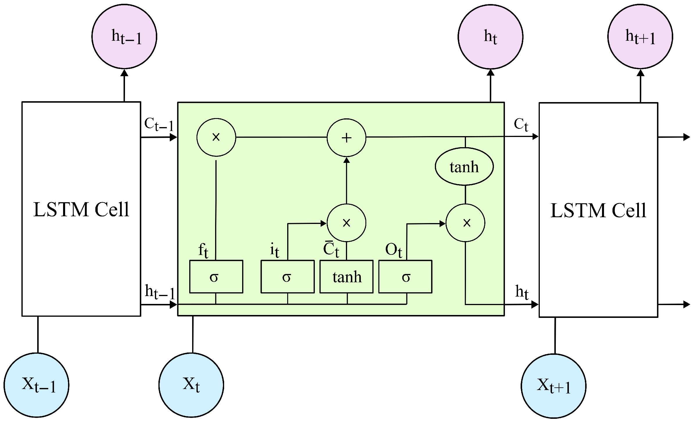
Figure 2 illustrates the basic architecture of an LSTM unit. Each LSTM unit typically has three gates: forget gate, input gate, and output gate. In the LSTM model, each time step comprises a specific component known as the cell state (C). The cell state preserves and conveys information pertinent to long-term memory within the model. The input sequence is presented as X, and the output is presented as h.
LSTM cells update six parameters per time step. Equations (7) to (12) present the details of the six parameters. The first parameter for each cell, which governs the degree to which the previous cell state should be forgotten, is the forget gate parameter f t . In the given equations, weights are denoted by (W), and biases are denoted by (b). The input gate serves as the second parameter in an LSTM cell, playing a crucial role in deciding the new information to be added or retained in the cell state. C t ¯ represents the candidate values for the new cell state. Subsequently, the cell state C t is updated. Finally, the output parameter O t is computed. The final gate is the output gate, which governs the extraction of information from the cell state and subsequently determines the current step h t .
f t = σ ( W f . h t 1 , X t + b f )
i t = σ ( W i . h t 1 , X t + b i )
C t ¯ = t a n h ( W C . h t 1 , X t + b C )
C t = f t C t 1 + i t C t ¯
O t = σ ( W O . h t 1 , X t + b O )
h t = O t t a n h C t
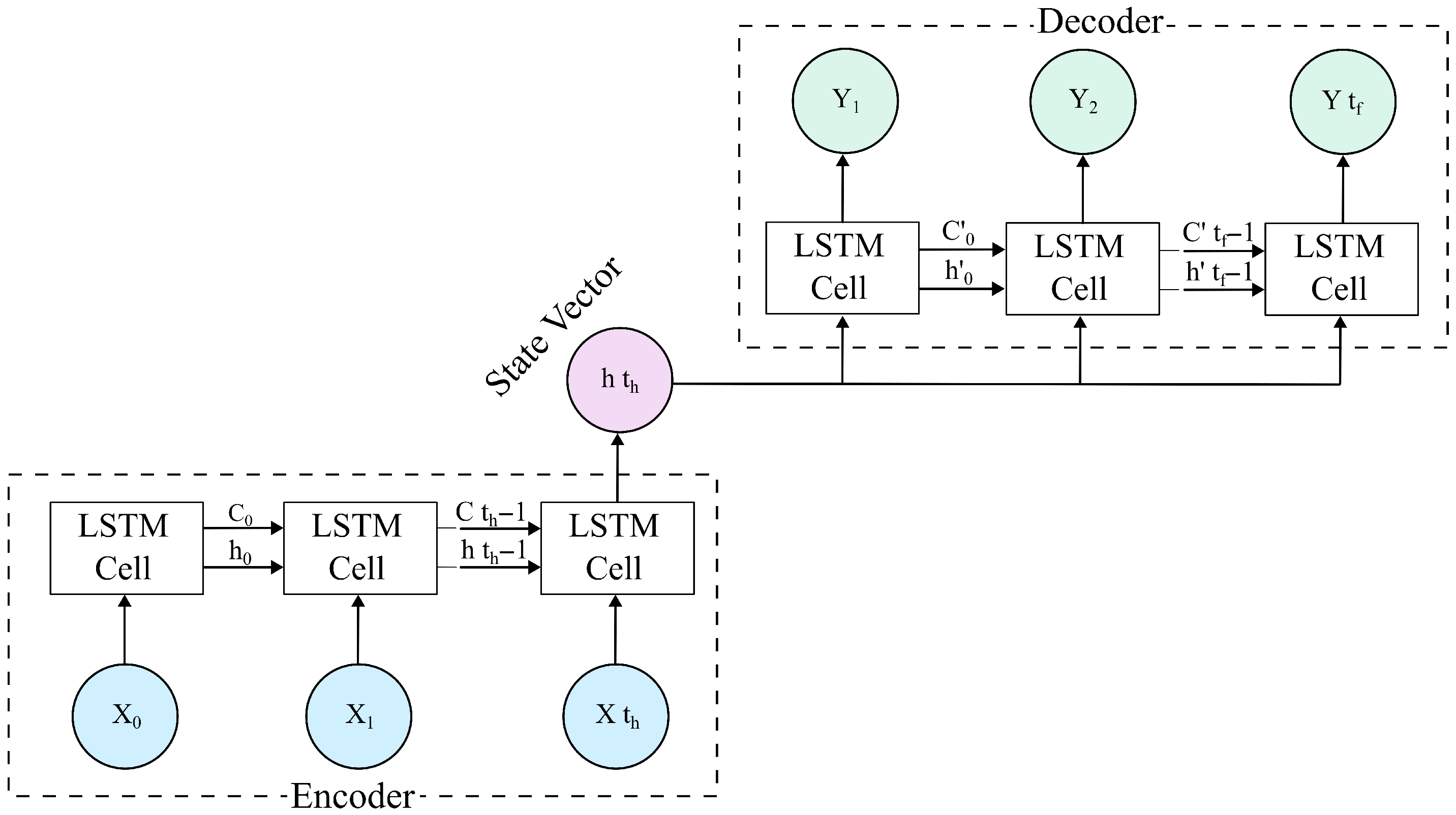
LSTM can address the issue of long-term dependencies, yet it is constrained by the requirement of having the same time steps for both input and output. Nonetheless, in contexts such as streamflow forecasting, as detailed in this paper, it is essential to include not just the rainfall data at the time steps we aim to predict but also the rainfall information from preceding hours. To address this issue, Sutskever et al. [43] introduced a neural network architecture known as encoder–decoder, enabling the model to operate with varying input and output time steps. As shown in Figure 3, the encoder LSTM for historical streamflow data in this study with t h time steps produces a final output h t h , which is stored in a cell called the state vector. This state vector is then utilized as input for the decoder LSTM, which operates with t f time steps.

4.2. Model Design

In this study, we developed an LSTM-based encoder–decoder model, as illustrated in Figure 4, for hourly streamflow predictions up to 12 h into the future. The input features include historical and forecasted rainfall data as well as historical streamflow data. In this model framework, input time series are processed separately due to variations in their lengths. The first LSTM encoder for the historical streamflow data has a length of t h = 60 , and the second LSTM encoder for the historical and forecasted rainfall data has a length of t h + t f = 72 . In this section, we assume that future rainfall can be accurately forecasted. Later, in Section 6, we will account for rainfall forecast errors or uncertainties. Following the LSTM-based encoder–decoder architecture, several dense layers are employed to output forecasted streamflow for up to t f = 12 h into the future.
We predominantly selected default settings and parameters for DL models available in TensorFlow-Keras. Each LSTM encoder layer contains 256 neurons, and the model includes a single LSTM decoder layer with 512 neurons. Following the decoder, there are six dense layers structured for time-series data, with neuron counts decreasing from 512 to 1. The ReLU activation function ( R ( y ) = m a x ( 0 , y ) ) is utilized in all dense layers. During the training phase, we implemented a dropout rate of 0.2 to mitigate overfitting and promote a sparse structure within the model. This dropout rate involved randomly deactivating 20 percent of the neural connections between nodes within the dense layers. The proposed DL model employs the mean squared error (MSE) as the loss function, defined as
MSE = 1 N i = 1 N ( Y i y i ) 2
where N is the number of samples, and Y i is the predicted value.
We employed the Adaptive Moment Estimation (Adam) optimization algorithm to minimize the loss function. The optimizer is initialized with a learning rate of 0.0001. During training, one out of every five instances in the dataset was allocated to the validation set after applying feature scaling using the MinMaxScaler. In this study, we performed model training, validation, and testing using Python (version 3.11.9), hosted on a machine with an Intel Core i7-12700K processor, an NVIDIA GeForce RTX 3070 Ti graphics card, and 64 GB of RAM.

4.3. Streamflow Prediction: Performance of Deterministic LSTMs

We evaluated the performance of deterministic LSTM models trained on three training datasets: the 20-event dataset (9600 samples), the 30-event dataset (14,400 samples), and the 40-event dataset (19,200 samples), as described in Section 3.3. An independent test set of 9600 samples was used to ensure a fair evaluation. Each LSTM model was trained following the procedure outlined in Section 4.2 and evaluated using the NSE metric as presented before (Equation (3)) with the difference that here we compare the HEC-HMS-simulated streamflow with the predicted streamflow generated by our developed model. The NSE in this context is defined as follows:
NSE = 1 i = 1 N ( Y i y i ) 2 i = 1 N ( y i y i ¯ ) 2
where y i ¯ denotes the average of simulated values.
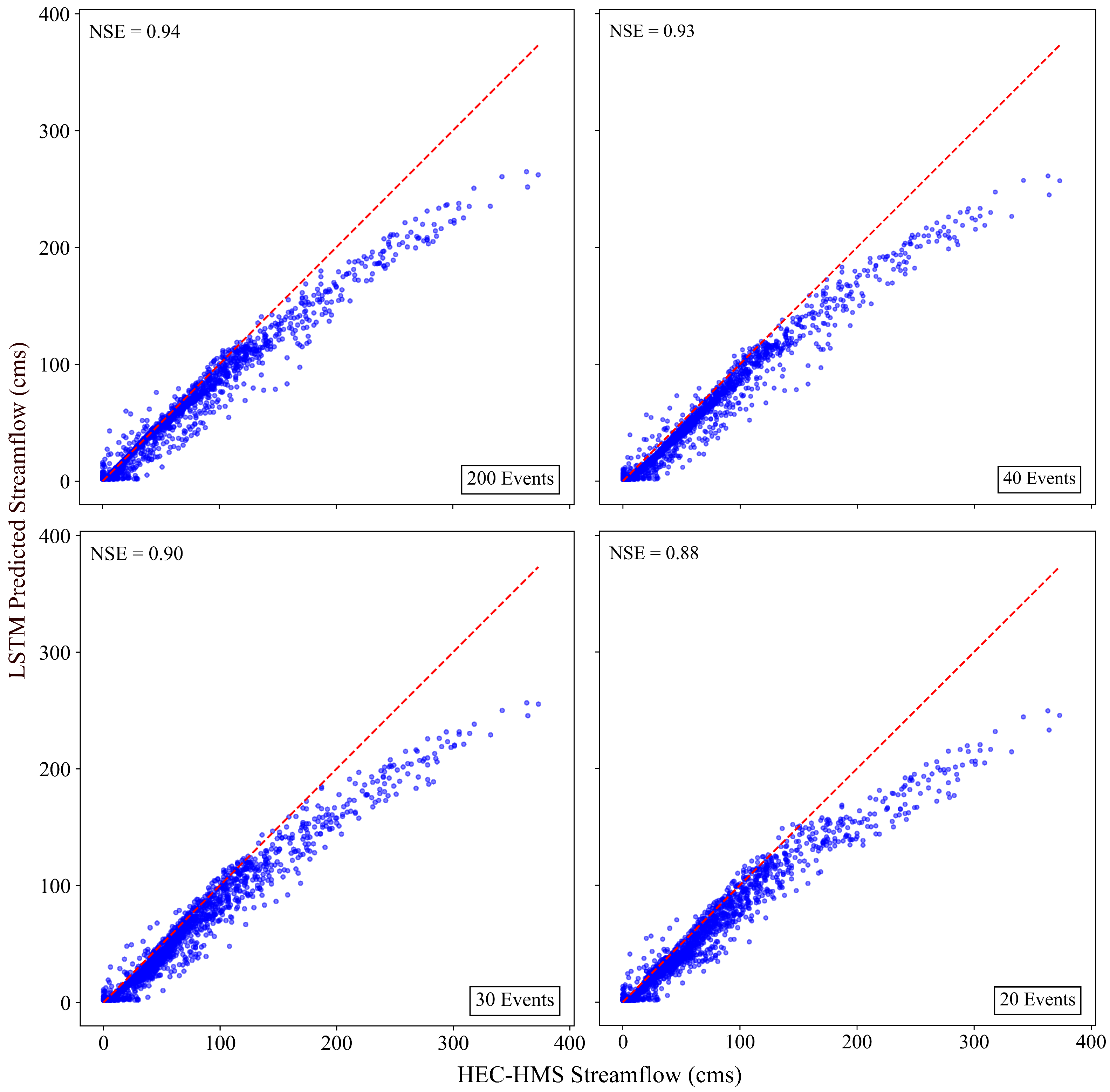
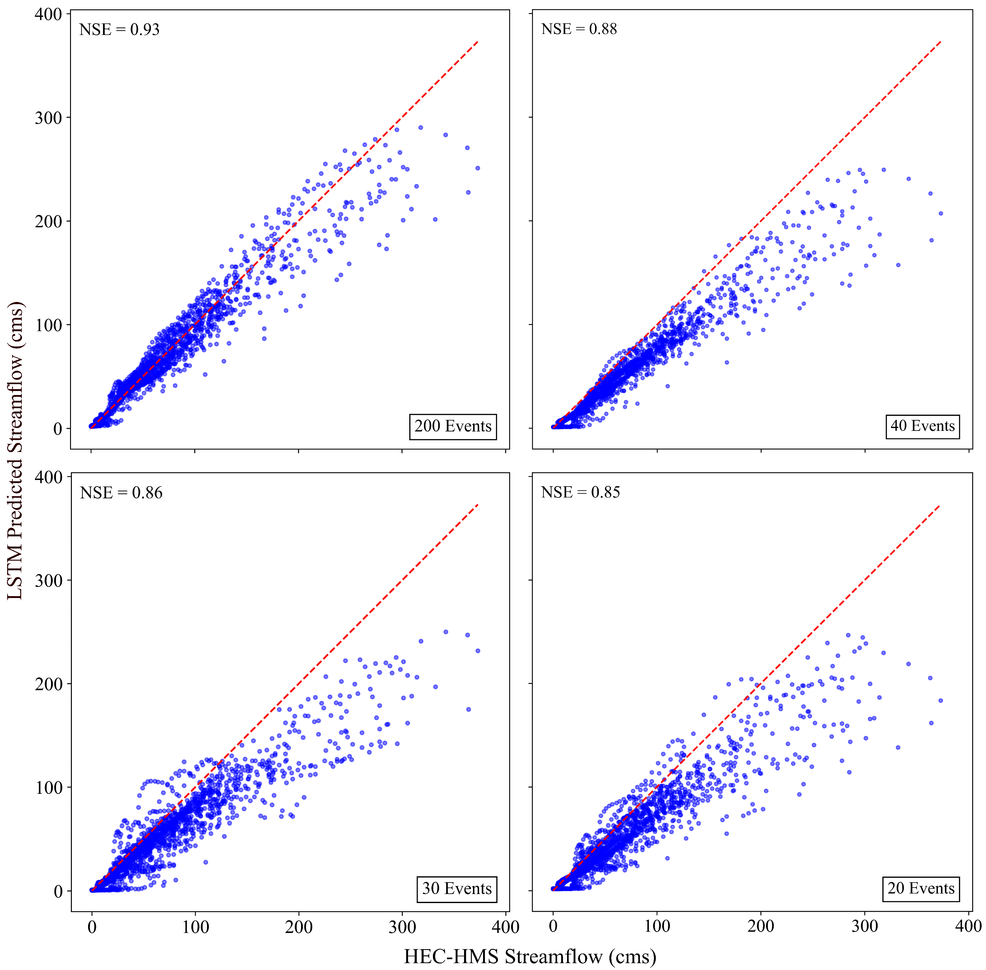
Additionally, we trained a benchmark model on a larger dataset, referred to as the 200-event dataset, containing 96,000 samples generated from the original pool of 200 rainfall events. Figure 5 and Figure 6 show the relationships between the LSTM model predictions and the HEC-HMS-simulated streamflow values on the test set at 1-h and 12-h lead times, respectively.
Figure 5 illustrates that all models trained with different sizes of training sets have high predictive accuracy, especially for low streamflow values (less than 155 cms). The model assessment revealed very high NSE values of 0.94 and 0.93 between the predicted and HEC-HMS-simulated streamflow values from the LSTMs trained on the 200- and 40-event datasets, respectively. For two other models, trained on 30- and 20-event datasets, although plots show marginally lower NSE scores of 0.90 and 0.88 compared to the earlier ones, they still remain indicative of a strong correlation. For the predictions with a lead time of 12 h, Figure 6 depicts the same pattern as in Figure 5. However, the NSE values are slightly lower than those for the 1-h lead time predictions, with the model trained with the 200-event dataset outperforming the others.
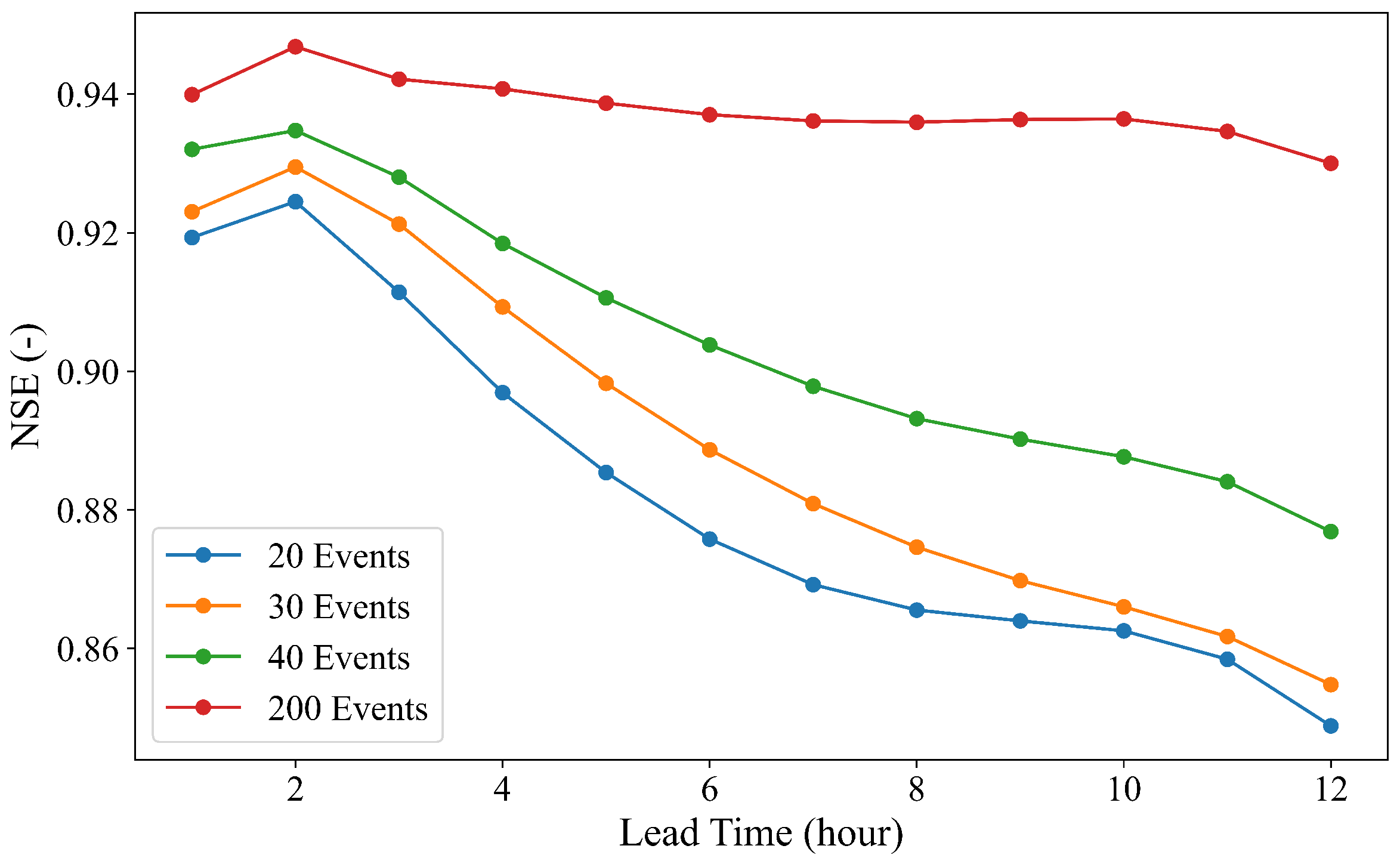
We also calculated the NSEs to assess every LSTM across various lead times, as illustrated in Figure 7. Overall, all models achieved NSE values higher than 0.85, demonstrating strong predictive capabilities. The models performed exceptionally well at shorter lead times and maintained high accuracy up to 12 h ahead. In this context, the model trained with the 200-event dataset outperformed the other three models. Although the model trained with the 40-event dataset did not reach the performance level of the 200-event model, it still achieved high NSE values across all lead times compared to models trained with fewer events, indicating its substantial predictive skill.
These findings suggest that, while the 200-event dataset yields the highest accuracy, the 40-event dataset offers a practical alternative, striking an optimal balance between performance and training efficiency. It provides sufficient data for effective training without overfitting and leads to better generalization and predictive performance. Consequently, the 40-event training set has been selected for further model improvement and analysis.

5. Streamflow Prediction with Emphasizing Peak Values

This section introduces two distinct loss functions designed to improve the performance of LSTMs in accurately capturing high streamflow values during peak flow events. Traditional loss functions, such as MSE, often struggle to emphasize extreme values, leading to the underestimation of peak flows. To address this limitation, we propose loss functions that prioritize high streamflow values, enhancing the model’s ability to learn and predict extreme hydrological events more effectively.

5.1. Proposed LSTMs to Capture Higher Streamflow Values

In Figure 5 and Figure 6, noticeable underestimations can be observed at higher streamflow values, a common issue in ML-based streamflow predictions when using MSE as a loss function [44]. Considering high streamflow values (>155 cms) only in the test set, the NSE could be as low as −0.90, meaning that the model prediction was worse than simply using the average value. This suggests that, while the overall accuracy was high, the ML model struggled with predicting higher streamflow values.
The MSE, as a symmetric loss function, treats all errors equally and emphasizes reducing the average error. This can disproportionately penalize larger errors, leading the model to prioritize minimizing errors for more frequent low streamflow values and potentially underestimate peak streamflow events. This underestimation is problematic in hydrological applications where accurately predicting peak values is crucial for flood warning systems and water resource management. To address this limitation, we introduce two asymmetric loss functions for our LSTM model to better capture higher streamflow values.
In contrast to symmetric loss functions, asymmetric loss functions are designed to handle cases where overestimations and underestimations have different consequences, thus assigning different penalties to these errors. This can improve the models’ ability to predict higher values. This concept is rooted in several well-established practices, particularly in fields like economics, finance, and the power and energy sectors [45,46,47,48]. However, in the realm of hydrological forecasting, there are relatively fewer studies on this subject. We will highlight these studies in the following subsections.

5.1.1. LSTM with a Pinball Loss Function

When dealing with scenarios where the distribution of the target variable (the streamflow hydrograph) is non-Gaussian or skewed, the PL, also known as the quantile regression loss, can be used as an alternative [49]. This loss function assigns penalties to errors depending on the selected quantile. In the field of streamflow forecasting, the PL has been utilized in a limited number of studies within probabilistic frameworks for estimating the conditional quantiles of streamflow forecasts [30,50,51]. However, in our specific case, we have used the PL in a deterministic LSTM framework with the goal of enhancing the model’s ability to predict peak streamflow events more accurately. We chose 0.8 and 0.9 quantiles, focusing on the upper end of the distribution to penalize underestimations. The PL function for a given quantile is defined as
PL ( y , Y ) = 1 N i = 1 N q · ( y i Y i ) · 1 ( y i > Y i ) + ( 1 q ) · ( Y i y i ) · 1 ( y i Y i )
where 1 ( · ) is the indicator function, which is 1 if the condition inside the parentheses is true and 0 otherwise. q is the selected quantile. If choosing the 0.8 quantile ( q = 0.8 ), this function penalizes underestimations Y i < y i much more heavily than overestimations Y i > y i , with weights of 0.8 and 0.2, respectively.
Figure 8 shows the performance of LSTM models using two different loss functions: PL and MSE. The comparisons are conducted for two different quantiles (0.8 and 0.9) and two different lead times (1 h and 12 h). Also, Table 3 presents the performance metrics for the entire test set, as well as for instances where the simulated streamflow values were higher than 155 cms. As we can see, in the case of q = 0.9 , the model shows better overall performance (higher NSE) in capturing the variance of the simulated streamflow, with minimal scatter at the lead time of 1 h, particularly at higher streamflow values compared to MSE and PL with q = 0.8. This interpretation is consistent with the lead time of 12 h. However, as in Table 3, for streamflow values higher than 155 cms, the negative NSE values for a lead time of 12 h indicate that even the model with PL ( q = 0.9 ) has difficulty capturing these values at longer lead times.

5.1.2. LSTM with an Asymmetric Peak Loss Function

We demonstrated that the PL function did not perform well in predicting high streamflow values at longer lead times. In this section, we developed an alternative approach, focusing more on improving the accuracy of peak value predictions. Our approach combined traditional loss functions (MSE) with additional terms that emphasize higher values. Specifically, we modified the MSE to be asymmetric by incorporating an additional penalty for errors when the simulated streamflow exceeds a certain threshold.
To implement this idea, we defined a peak threshold (T) and an asymmetry factor (F) in the new loss function and adjusted them to best suit our data and prediction goals. We named our implementation of this asymmetric loss function asymmetric peak (AP), which is defined as follows:
AP ( y , Y ) = 1 N i = 1 N ( y i Y i ) 2 + 1 N i = 1 N ( y i Y i ) 2 · F · 1 ( y i > T ) · 1 ( y i > Y i )
where T = 0.45 (normalized streamflow equal to 155 cms) and F = 3.0 were chosen based on model tuning.
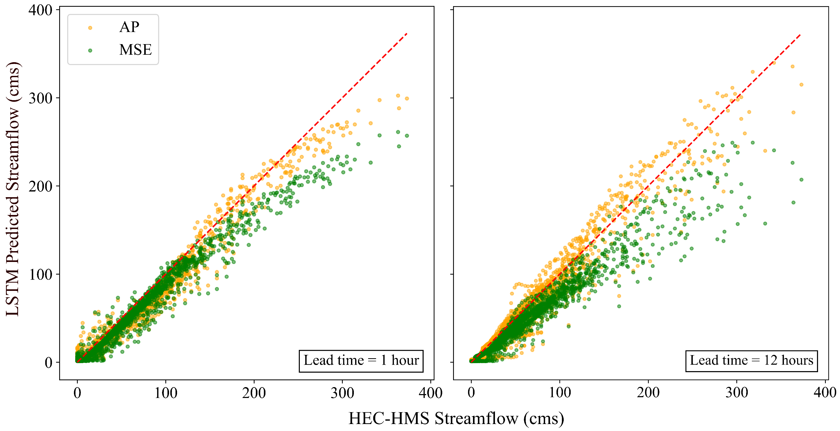
Figure 9 shows the prediction performance of LSTM with the proposed loss function compared to the ones with the conventional MSE at the lead times of 1 h and 12 h. The figure clearly illustrates that the model with AP captured the higher streamflow values more effectively at both lead times, aligning with its purpose. Additionally, Table 4, representing the performance metrics of LSTM models with three different loss functions, highlights the strength of the LSTM with AP, even at the lead time of 12 h.
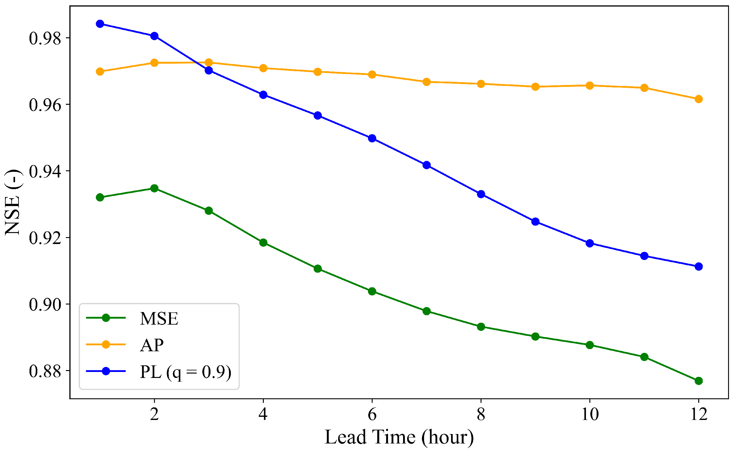
To comprehensively compare the impacts of different loss functions across various lead times, Figure 10 is presented. It can be concluded that LSTMs with the proposed AP and the PL (q = 0.9) loss functions outperformed the LSTM model with the conventional MSE loss function at all lead times. Although the model with the PL loss function performed slightly better at shorter lead times (up to 3 h), the LSTM model with the proposed AP loss function demonstrated superior performance overall. In summary, the AP loss function emerged as the best performer for the LSTM model, consistently achieving high NSE values across all lead times and proving to be the most reliable choice for long-term predictions.

6. Streamflow Prediction with Rainfall Forecast Uncertainties

In the above studies, we have assumed that future rainfall forecasts are precise in our deterministic LSTM. However, this assumption does not hold in real-world applications, where rainfall forecast uncertainty is both substantial and often the primary source of uncertainty in streamflow forecasting. To address this issue, we developed a PLSTM for streamflow forecasting. In our approach, we first used archived rainfall forecast data along with subsequent actual observations to analyze the errors in rainfall forecasts. This uncertainty was then integrated into both the training and test datasets to better reflect real-world forecasting conditions. Utilizing our probabilistic LSTM model, we systematically quantified the uncertainty in streamflow predictions, extending up to 12 h into the future. By accounting for forecast uncertainty, our approach enhances the robustness and reliability of streamflow predictions, ultimately improving the model’s ability to support early warning systems and flood risk management.

6.1. Rainfall Forecast Error Analysis

We analyzed the errors (uncertainties) in the forecasted rainfall over the next 12 h. To achieve this, we first obtained archived rainfall forecasts from January to November 2020 for the subbasin encompassing Iowa City from the High-Resolution Rapid Refresh (HRRR) model. The HRRR, developed by NOAA, is a real-time convection-allowing atmospheric model with 3-kilometer spatial resolution and hourly updates, initialized on 3-kilometer grids incorporating radar data assimilation [52]. HRRR produces deterministic forecasts every hour out to 18 h for the continental United States (CONUS). We also obtained point observation data for the same period from the Iowa Environmental Mesonet [53]. Figure 11 illustrates the time series of 1 h into future rainfall forecasts versus the observed rainfall (top plot) at the Iowa City weather station. The corresponding time series of errors during the same period is also presented in Figure 11 (bottom plot).
We defined errors as the difference between observed and forecasted rainfall, with negative errors indicating overestimations and positive errors implying underestimations. Although we have presented the results for just one-hour-ahead forecasts in this section, it is important to highlight that the average errors increased with lead times from 1 h to 12 h into the future.
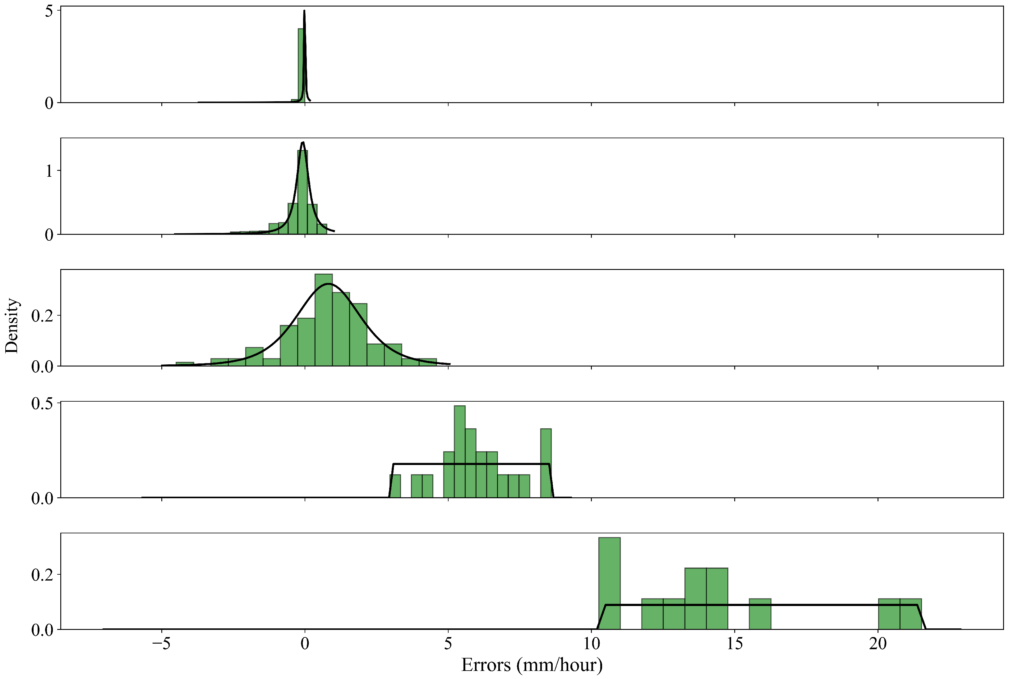
We then stratified the observed rainfall values into five categories: no rainfall ( rainfall = 0 ( mm / hour ) , 6525 data points); light ( 0 < rainfall < 1 , 593 data points); moderate ( 1 rainfall < 5 , 137 data points); heavy ( 5 rainfall < 10 , 27 data points); and very heavy ( rainfall 10 , 14 data points). Subsequently, we fitted a distribution to the corresponding errors in each rainfall category. Figure 12 depicts the histogram of the errors and the fitted distributions for defined categories at the lead time of 1 h. It can be observed that underforecasting consistently occurs for heavy and very heavy rainfall.
Across all lead times up to 12 h, the best-fit probability distributions for the first three categories were normal distributions, whereas the “very heavy” category was best represented by a uniform distribution. For the fourth category, i.e., “heavy”, the type of distribution varied with lead time, with both normal and uniform distributions being selected accordingly.

6.2. Probabilistic LSTM

In previous sections, our discussion was centered on deterministic LSTM models, which provide point estimates of streamflow up to 12 h ahead. These models are limited in accounting for uncertainties, especially those in rainfall forecasts, and fail to offer a range of potential outcomes. Presenting a range of plausible scenarios is critical for informed and risk-aware decision-making. Therefore, advancing to PLSTM models is a necessary progression to address these constraints, enhancing the robustness and reliability of streamflow predictions.
We have constructed the PLSTM with NLL as the loss function, which involves training the model to directly optimize the log-likelihood of the observed data under the predicted probability distribution. This function’s most general form is presented in Equation (17), which is minimized during the model training process.
NLL = i = 1 N log P ( y i | θ )
Here, N is the number of samples, P is the probability density function (PDF) of the predicted distribution, and θ indicates the parameters of P.
Considering that streamflow values cannot be negative, we opted for the log-normal distribution. The probability density function of this distribution is defined as
P ( y i ) = 1 y i σ i 2 π exp ( ln y i μ i ) 2 2 σ i 2
where μ i is the location parameter, and σ i is the scale parameter.
Our PLSTM model uses the same input features as the deterministic LSTM, with separate LSTM encoders for historical streamflow and combined historical and forecasted rainfall inputs. However, in this study, we analyze the errors in rainfall forecasts, as discussed in Section 6.1, and introduce sampled noise into the rainfall data as input for the model. The encoder outputs are combined into a unified state vector, which is processed through an LSTM decoder and dense layers to predict the means and standard deviations of log-normal distributions, thereby providing confidence intervals for future streamflow predictions rather than single-point estimates.
This enables the model to capture both the expected values and associated uncertainties, providing confidence intervals rather than single-point estimates. The model closely follows the standard LSTM setup, but, as we mentioned above, it incorporates the NLL as the loss function. Additionally, the initial learning rate for the Adam optimizer is set to 0.0001.

6.3. Performance Evaluation Metrics

To evaluate the forecasts, we used established deterministic and probabilistic metrics from the hydrological modeling literature [24,51]. Reported metrics pertain to the test set, which was not used to train the model or tune hyperparameters.
Here, we employed NSE (Equation (14)), where the HEC-HMS-simulated streamflow is compared with the mean predicted streamflow generated by the PLSTM.
For evaluating probabilistic forecasts, we adopted three metrics: the continuous rank probability score (CRPS), the prediction interval coverage probability (PICP), and the mean prediction interval width (MPIW), as described below.
CRPS Equation (19) compares the forecasted and observed cumulative distribution functions (CDFs), providing a measure of how well the forecasted distribution matches the actual outcome. CRPS values range from 0 to infinity, with lower values indicating better prediction accuracy.
CRPS = 1 N i = 1 N F ( Y i ) 1 ( Y i y i ) 2 d y
In this equation, F( Y i ) is the forecasted CDF.
PICP Equation (20) measures the proportion of observed data points that fall within the predicted intervals. A higher PICP indicates better reliability of the prediction intervals in capturing the true values. PICP values range from 0 to 1, where 1 indicates that all observed values fall within their respective prediction intervals.
PICP = 1 N i = 1 N 1 ( L i y i U i )
L i and U i represent the lower and upper bounds of the prediction interval, respectively.
MPIW Equation (21) evaluates the average width of prediction intervals. It provides an indication of the uncertainty in predictions. Narrower intervals suggest higher confidence, while wider intervals indicate greater uncertainty.
MPIW = 1 N i = 1 N ( U i L i )
As discussed so far, the uncertainty in forecasted rainfalls up to 12 h into the future was integrated into the PLSTM model to output the predicted means and standard deviations of future streamflow values.
Figure 13 illustrates the comparison between HEC-HMS-simulated streamflow and predicted streamflow using the PLSTM model at 1-h and 12-h lead times. Both plots exhibit a general positive correlation, underscoring the model’s proficiency in capturing streamflow trends. The shaded regions denote the 95 percent prediction interval, which expands at higher values of predicted streamflow, indicating increased uncertainty at these levels.
At the 1-h lead time, the model produces relatively narrow prediction intervals, particularly at lower streamflow values; the majority of the simulated streamflow values fall within these prediction intervals and closely align with the 1:1 line (red dashed line), indicating high prediction accuracy and confidence. Heavy rainfall usually leads to high streamflow. Consequently, prediction intervals widen at high streamflow values due to larger forecast errors associated with heavy and very heavy rainfall.
Conversely, the 12-h lead time plot reveals broader prediction intervals and a greater dispersion of data points around the 1:1 line, reflecting the increasing uncertainty associated with longer-term forecasts. Nonetheless, the prediction intervals continue to encompass a substantial portion of the simulated values, highlighting the model’s capabilities even at extended lead times.
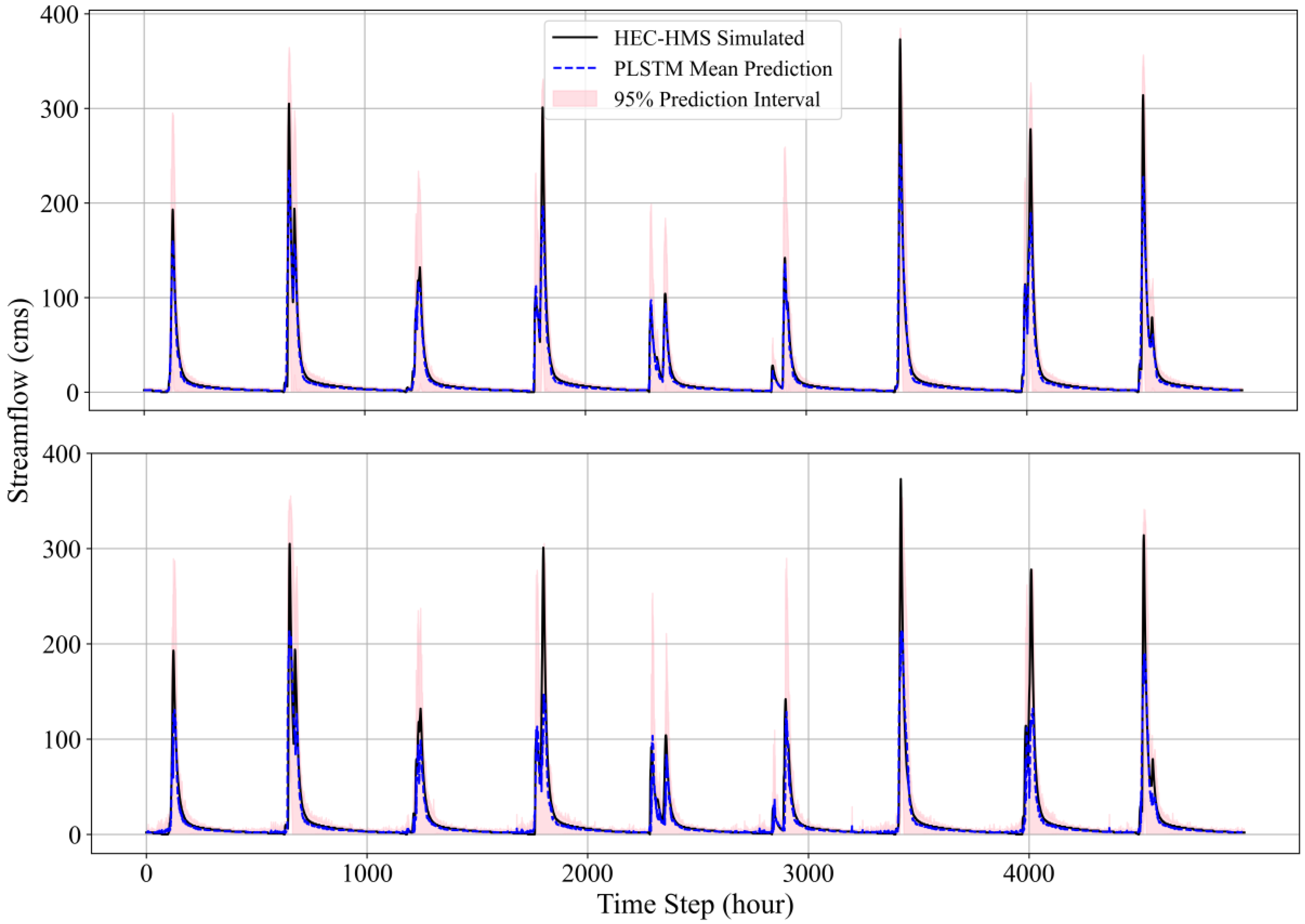
Also, Figure 14 presents point-wise predictions for several events in the test set at both 1-h and 12-h lead times, offering a clear visual assessment of the PLSTM model’s predictive skill. The model effectively reproduces the shape and timing of streamflow peaks while maintaining well-calibrated probabilistic forecasts, with the majority of simulated streamflow values falling within the shaded 95 percent prediction intervals. As expected, the prediction intervals widen at the 12-h lead time, and discrepancies between the PLSTM mean predictions and the HEC-HMS-simulated streamflow—particularly around peak flows—become more pronounced. Overall, these results demonstrate the model’s capability to reliably capture both the temporal dynamics and predictive uncertainty of streamflow across diverse hydrologic scenarios and lead times.
Table 5 presents the performance metrics of the PLSTM model for lead times up to 12 h, complementing the insights from Figure 13 and Figure 14. Note that higher values of NSE and PICP and lower values of MPIW and CRPS indicate better probabilistic model performance. The NSE for mean streamflow forecasts decreases from 0.9451 to 0.735 as the lead time increases from 1 to 12 h, highlighting a decline in predictive accuracy over longer lead times. The PICP values consistently remain above 0.9789, indicating that the 95 percent prediction intervals reliably encompass the true streamflow values across all the lead times. Although there is a slight decrease at longer lead times, the model continues to maintain good coverage. The MPIW values increase from 24.835 to 26.131 as the lead time extends from 1 to 12 h. This observed increase in MPIW signifies diminishing confidence in the model’s predictions as lead time increases.

7. Conclusions and Outlook

This study proposes three advanced ML techniques to enhance data-driven streamflow forecasting. First, AL was employed to optimally select rainfall events, minimizing the efforts of hydrological modeling and simulations required for data generation. The LSTM trained with 40 selected rainfall events from a pool of 200 randomly generated events achieved NSE values of 0.93 and 0.88 at 1-h and 12-h lead times, respectively—only marginally lower (by less than 1% and 5%) than the model trained with all 200 events. This finding demonstrates that a substantially smaller yet strategically selected training set can preserve predictive accuracy comparable to that of a fully trained model. Overall, this approach effectively identified the most informative rainfall events for model training while markedly reducing computational cost and data generation time.
Secondly, we introduced a novel loss function tailored specifically for peak streamflow prediction. By incorporating the developed asymmetric peak (AP) loss function, the model achieved substantial quantitative improvements over the conventional MSE loss. At a 1-h lead time, the AP-based model improved the overall NSE from 0.93 to 0.97 (a 4.3% increase) and peak-flow NSE from 0.12 to 0.76—representing more than a sixfold improvement in capturing high-flow values. Similarly, at a 12-h lead time, the AP loss enhanced the overall NSE from 0.88 to 0.96 (a 9.1% increase) and peak-flow NSE from –0.90 to 0.62, demonstrating a complete reversal from poor to highly reliable peak predictions. These findings confirm that AP loss delivers superior skill in capturing high streamflow values, effectively addressing one of the most critical challenges in hydrological forecasting. Additionally, the developed loss function outperformed the state-of-the-art PL function and holds promise for applications in ML models in other domains, such as economics and finance.
Lastly, we developed and implemented a probabilistic LSTM model that effectively incorporates rainfall forecast errors into streamflow predictions. The model achieved PICP higher than 0.97, NSE decreasing from 0.94 to 0.73, CRPS increasing from 2.26 to 4.24, and MPIW increasing from 24.835 to 26.131 across lead times up to 12 h, offering well-calibrated uncertainty quantification while maintaining high predictive skill. These contributions collectively improve the accuracy, reliability, and practical utility of streamflow forecasts, providing valuable insights for decision-making and flood management efforts.
While this research primarily focused on streamflow forecasting, the proposed methods can be applied to predict crucial variables in various related fields, including meteorology (wind speed and precipitation), environmental science (nitrate concentration), water resource management (reservoir levels and water demand), and agriculture (evapotranspiration).
In the current study, only one outflow configuration (gates fully open and initially zero storage) was considered. Building on the strengths of our approach, future research will explore additional configurations. While rainfall events were limited to 3 days for data generation in this study, the approach can be easily extended to events of varying lengths. Additionally, to improve the performance of our PLSTM model at longer lead times, we are considering investigating the effect of combining NLL and AP loss functions. These directions aim to refine our models further and enhance their applicability across diverse scenarios. Furthermore, alternative architectures, such as GRU, CNN, and Transformer networks, will be explored for comparative analysis and potential model improvement.

Author Contributions

Conceptualization, S.T., R.M., F.G. and S.X.; methodology, S.T. and S.X.; software, S.T.; validation, S.T.; formal analysis, S.T.; investigation, S.T. and S.X.; resources, S.T., R.M., F.G. and S.X.; data curation, S.T.; writing—original draft preparation, S.T.; writing—review and editing, S.T., R.M., F.G. and S.X.; visualization, S.T.; supervision, R.M. and S.X.; project administration, S.X.; funding acquisition, S.X. All authors have read and agreed to the published version of the manuscript.

Funding

This material is based upon work supported by the National Science Foundation under Grant Number 2226936 and the U.S. Department of Education under Grant Number ED#P116S210005. Any opinions, findings, and conclusions, or recommendations expressed in this material are those of the author(s) and do not necessarily reflect the views of the National Science Foundation and the U.S. Department of Education.

Institutional Review Board Statement

Not applicable.

Informed Consent Statement

Not applicable.

Data Availability Statement

The data supporting this study are available from the author’s GitHub repository at https://github.com/soheylam/LSTM_PLSTM_ActiveLearning (accessed on 28 October 2025).

Acknowledgments

During the preparation of this manuscript/study, the author(s) used GPT-3.5 and GPT-4 for the purposes of improving the readability and language. The authors have reviewed and edited the output and take full responsibility for the content of this publication.

Conflicts of Interest

The authors declare no conflicts of interest.

Abbreviations

The following abbreviations are used in this manuscript:
MLMachine learning
SSTStochastic storm transposition
LSTMLong short-term memory
AIArtificial intelligence
SVMsSupport vector machines
DLDeep learning
RNNsRecurrent neural networks
SWATSoil water assessment tool
ALActive learning
PLPinball loss
PLSTMProbabilistic long short-term memory
NLLNegative log-likelihood
HMSHydrologic modeling system
DEMDigital elevation model
SCSSoil conservation service
CNCurve number
NSENash–Sutcliffe efficiency
RSRRoot mean squared error ratio
PBIASPercent bias
GSGreedy sampling
APAsymmetric peak
CRPSContinuous rank probability score
PICPPrediction interval coverage probability
MPIWMean prediction interval width

References

  1. Zhao, X.; Lv, H.; Wei, Y.; Lv, S.; Zhu, X. Streamflow forecasting via two types of predictive structure-based gated recurrent unit models. Water 2021, 13, 91. [Google Scholar] [CrossRef]
  2. Nguyen, H.D.; Pham Van, C.; Nguyen, Q.-H.; Bui, Q.-T. Daily streamflow prediction based on the long short-term memory algorithm: A case study in the Vietnamese Mekong Delta. J. Water Clim. Change 2023, 14, 1247–1267. [Google Scholar] [CrossRef]
  3. Farfán-Durán, J.F.; Cea, L. Streamflow forecasting with deep learning models: A side-by-side comparison in Northwest Spain. Earth Sci. Inform. 2024, 17, 5289–5315. [Google Scholar] [CrossRef]
  4. Yifru, B.A.; Lim, K.J.; Lee, S. Enhancing streamflow prediction physically consistently using process-based modeling and domain knowledge: A review. Sustainability 2024, 16, 1376. [Google Scholar] [CrossRef]
  5. Zhang, J.; Chen, X.; Khan, A.; Zhang, Y.; Kuang, X.; Liang, X.; Taccari, M.; Nuttall, J. Daily runoff forecasting by deep recursive neural network. J. Hydrol. 2021, 596, 126067. [Google Scholar] [CrossRef]
  6. Sarker, S.; Leta, O.T. Review of watershed hydrology and mathematical models. Eng 2025, 6, 129. [Google Scholar] [CrossRef]
  7. Paniconi, C.; Lauvernet, C.; Rivard, C. Exploration of coupled surface–subsurface hydrological model responses and challenges through catchment- and hillslope-scale examples. Front. Water 2025, 7, 1553578. [Google Scholar] [CrossRef]
  8. Xia, Q.; Fan, Y.; Zhang, H.; Jiang, C.; Wang, Y.; Hua, X.; Liu, D. A review on the development of two-way coupled atmospheric-hydrological models. Sustainability 2023, 15, 2803. [Google Scholar] [CrossRef]
  9. Jahanbani, H.; Ahmed, K.; Gu, B. Data-driven artificial intelligence-based streamflow forecasting: A review of methods, applications, and tools. JAWRA J. Am. Water Resour. Assoc. 2024, 60, 1095–1119. [Google Scholar] [CrossRef]
  10. Granata, F.; Gargano, R.; De Marinis, G. Support vector regression for rainfall-runoff modeling in urban drainage: A comparison with the EPA’s storm water management model. Water 2016, 8, 69. [Google Scholar] [CrossRef]
  11. Yan, J.; Jin, J.; Chen, F.; Yu, G.; Yin, H.; Wang, W. Urban flash flood forecast using support vector machine and numerical simulation. J. Hydroinform. 2018, 20, 221–231. [Google Scholar] [CrossRef]
  12. Shi, T.; Shide, K. A comparative analysis of LSTM, GRU, and Transformer models for construction cost prediction with multidimensional feature integration. J. Asian Archit. Build. Eng. 2025, 1–16. [Google Scholar] [CrossRef]
  13. Xiao, J.; Deng, T.; Bi, S. Comparative analysis of LSTM, GRU, and Transformer models for stock price prediction. In Proceedings of the International Conference on Digital Economy, Blockchain and Artificial Intelligence, Guangzhou, China, 23–25 August 2024; pp. 103–108. [Google Scholar]
  14. Kratzert, F.; Klotz, D.; Brenner, C.; Schulz, K.; Herrnegger, M. Rainfall–runoff modelling using long short-term memory (LSTM) networks. Hydrol. Earth Syst. Sci. 2018, 22, 6005–6022. [Google Scholar] [CrossRef]
  15. Xiang, Z.; Yan, J.; Demir, I. A rainfall-runoff model with LSTM-based sequence-to-sequence learning. Water Resour. Res. 2020, 56, e2019WR025326. [Google Scholar] [CrossRef]
  16. Guo, Y.; Yu, X.; Xu, Y.; Chen, H.; Gu, H.; Xie, J. AI-based techniques for multi-step streamflow forecasts: Application for multi-objective reservoir operation optimization and performance assessment. Hydrol. Earth Syst. Sci. 2021, 25, 5951–5979. [Google Scholar] [CrossRef]
  17. Yin, H.; Wang, F.; Zhang, X.; Zhang, Y.; Chen, J.; Xia, R.; Jin, J. Rainfall-runoff modeling using long short-term memory based step-sequence framework. J. Hydrol. 2022, 610, 127901. [Google Scholar] [CrossRef]
  18. Luppichini, M.; Barsanti, M.; Giannecchini, R.; Bini, M. Deep learning models to predict flood events in fast-flowing watersheds. Sci. Total Environ. 2022, 813, 151885. [Google Scholar] [CrossRef]
  19. Hunt, K.M.R.; Matthews, G.R.; Pappenberger, F.; Prudhomme, C. Using a long short-term memory (LSTM) neural network to boost river streamflow forecasts over the western United States. Hydrol. Earth Syst. Sci. 2022, 26, 5449–5472. [Google Scholar] [CrossRef]
  20. Arsenault, R.; Martel, J.; Brunet, F.; Brissette, F.; Mai, J. Continuous streamflow prediction in ungauged basins: Long short-term memory neural networks clearly outperform traditional hydrological models. Hydrol. Earth Syst. Sci. 2023, 27, 139–157. [Google Scholar] [CrossRef]
  21. Chen, S.; Huang, J.; Huang, J. Improving daily streamflow simulations for data-scarce watersheds using the coupled SWAT-LSTM approach. J. Hydrol. 2023, 622, 129734. [Google Scholar] [CrossRef]
  22. Tursun, A.; Xie, X.; Wang, Y.; Liu, Y.; Peng, D.; Rusuli, Y.; Zheng, B. Reconstruction of missing streamflow series in human-regulated catchments using a data integration LSTM model. J. Hydrol. Reg. Stud. 2024, 52, 101744. [Google Scholar] [CrossRef]
  23. Klotz, D.; Kratzert, F.; Gauch, M.; Sampson, A.K.; Brandstetter, J.; Klambauer, G.; Hochreiter, S.; Nearing, G. Uncertainty estimation with deep learning for rainfall–runoff modeling. Hydrol. Earth Syst. Sci. 2022, 26, 1673–1693. [Google Scholar] [CrossRef]
  24. Jahangir, M.S.; Quilty, J. Generative deep learning for probabilistic streamflow forecasting: Conditional variational auto-encoder. J. Hydrol. 2024, 629, 130498. [Google Scholar] [CrossRef]
  25. Tran, V.N.; Dwelle, M.C.; Sargsyan, K.; Ivanov, V.Y.; Kim, J. A novel modeling framework for computationally efficient and accurate real-time ensemble flood forecasting with uncertainty quantification. Water Resour. Res. 2020, 56, e2019WR025727. [Google Scholar] [CrossRef]
  26. Delottier, H.; Doherty, J.; Brunner, P. Data space inversion for efficient uncertainty quantification using an integrated surface and sub-surface hydrologic model. Geosci. Model Dev. 2023, 16, 4213–4231. [Google Scholar] [CrossRef]
  27. Troin, M.; Arsenault, R.; Wood, A.W.; Brissette, F.; Martel, J. Generating ensemble streamflow forecasts: A review of methods and approaches over the past 40 years. Water Resour. Res. 2021, 57, e2020WR028392. [Google Scholar] [CrossRef]
  28. Hauswirth, S.M.; Bierkens, M.F.P.; Beijk, V.; Wanders, N. The suitability of a seasonal ensemble hybrid framework including data-driven approaches for hydrological forecasting. Hydrol. Earth Syst. Sci. 2023, 27, 501–517. [Google Scholar] [CrossRef]
  29. Hao, Y.; Baik, J.; Tran, H.; Choi, M. Quantification of the effect of hydrological drivers on actual evapotranspiration using the Bayesian model averaging approach for various landscapes over Northeast Asia. J. Hydrol. 2022, 607, 127543. [Google Scholar] [CrossRef]
  30. Jahangir, M.S.; You, J.; Quilty, J. A quantile-based encoder-decoder framework for multi-step ahead runoff forecasting. J. Hydrol. 2022, 619, 129269. [Google Scholar] [CrossRef]
  31. Haddad, K. A comprehensive review and application of Bayesian methods in hydrological modelling: Past, present, and future directions. Water 2025, 17, 1095. [Google Scholar] [CrossRef]
  32. Gurbuz, F.; Mudireddy, A.; Mantilla, R.; Xiao, S. Using a physics-based hydrological model and storm transposition to investigate machine-learning algorithms for streamflow prediction. J. Hydrol. 2024, 628, 130504. [Google Scholar] [CrossRef]
  33. Alabbad, Y.; Demir, I. Comprehensive flood vulnerability analysis in urban communities: Iowa case study. Int. J. Disaster Risk Reduct. 2022, 74, 102955. [Google Scholar] [CrossRef]
  34. U.S. Army Corps of Engineers, Rock Island District. Coralville Lake Water Control Plan Update Report with Integrated Environmental Assessment; U.S. Army Corps of Engineers: Rock Island, IL, USA, 2022. [Google Scholar]
  35. U.S. Army Corps of Engineers, Hydrologic Engineering Center. HEC-HMS User’s Manual, Version 4.13. Hydrol Eng Center: Davis, CA, USA. Available online: https://www.hec.usace.army.mil/confluence/hmsdocs/hmsum/latest (accessed on 11 October 2025).
  36. Moriasi, D.; Arnold, J.G.; Liew, M.W.V.; Bingner, R.L.; Harmel, R.D.; Veith, T.L. Model evaluation guidelines for systematic quantification of accuracy in watershed simulations. Trans. ASABE 2007, 50, 885–900. [Google Scholar] [CrossRef]
  37. Wright, D.B. RainyDay: Rainfall Hazard Analysis System. Available online: https://github.com/HydroclimateExtremesGroup/RainyDay (accessed on 20 September 2025).
  38. Wu, D.; Lin, C.; Huang, J. Active learning for regression using greedy sampling. Inf. Sci. 2019, 474, 90–105. [Google Scholar] [CrossRef]
  39. Bi, J.; Xu, Y.; Conrad, F.; Wiemer, H.; Ihlenfeldt, S. A comprehensive benchmark of active learning strategies with AutoML for small-sample regression in materials science. Sci. Rep. 2025, 15, 37167. [Google Scholar] [CrossRef]
  40. Chen, Y.; Deierling, P.; Xiao, S. Exploring active learning strategies for predictive models in mechanics of materials. Appl. Phys. A 2024, 130, 588. [Google Scholar] [CrossRef]
  41. Waqas, M.; Humphries, U.W. A critical review of RNN and LSTM variants in hydrological time series predictions. MethodsX 2024, 13, 102946. [Google Scholar] [CrossRef] [PubMed]
  42. Ni, L.; Wang, D.; Singh, V.P.; Wu, J.; Wang, Y.; Tao, Y.; Zhang, J. Streamflow and rainfall forecasting by two long short-term memory-based models. J. Hydrol. 2020, 583, 124296. [Google Scholar] [CrossRef]
  43. Sutskever, I.; Vinyals, O.; Le, Q.V. Sequence to sequence learning with neural networks. In Proceedings of the 28th International Conference on Neural Information Processing Systems, Montreal, QC, Canada, 8–13 December 2014; pp. 3104–3112. [Google Scholar]
  44. Gupta, H.V.; Kling, H.; Yilmaz, K.K.; Martinez, G.F. Decomposition of the mean squared error and NSE performance criteria: Implications for improving hydrological modelling. J. Hydrol. 2009, 377, 80–91. [Google Scholar] [CrossRef]
  45. Dessain, J. Improving the Prediction of Asset Returns with Machine Learning by Using a Custom Loss Function. Adv. Artif. Intell. Mach. Learn. 2023, 3, 1640–1653. [Google Scholar] [CrossRef]
  46. Wang, Y.; Gan, D.; Sun, M.; Zhang, N.; Lu, Z.; Kang, C. Probabilistic individual load forecasting using pinball loss guided LSTM. Appl. Energy 2019, 235, 10–20. [Google Scholar] [CrossRef]
  47. Wu, J.; Wang, Y.; Tian, Y.; Burrage, K.; Cao, T. Support vector regression with asymmetric loss for optimal electric load forecasting. Energy 2021, 223, 119969. [Google Scholar] [CrossRef]
  48. Zhang, J.; Wang, Y.; Hug, G. Cost-oriented load forecasting. Electr. Power Syst. Res. 2022, 205, 117723. [Google Scholar] [CrossRef]
  49. Tagasovska, N.; Lopez-Paz, D. Single-model uncertainties for deep learning. In Proceedings of the 33rd International Conference on Neural Information Processing Systems, Vancouver, BC, Canada, 8–14 December 2019; pp. 6417–6428. [Google Scholar]
  50. Tyralis, H.; Papacharalampous, G. Quantile-based hydrological modelling. Water 2022, 13, 3420. [Google Scholar] [CrossRef]
  51. Cao, C.; He, Y.; Cai, S. Probabilistic runoff forecasting considering stepwise decomposition framework and external factor integration structure. Expert Syst. Appl. 2024, 236, 121350. [Google Scholar] [CrossRef]
  52. NOAA. HRRR: High-Resolution Rapid Refresh. Available online: https://rapidrefresh.noaa.gov/hrrr/ (accessed on 11 October 2025).
  53. Iowa Environmental Mesonet. ASOS/AWOS Hourly Precipitation Data. Available online: https://mesonet.agron.iastate.edu/request/asos/hourlyprecip.phtml (accessed on 11 October 2025).
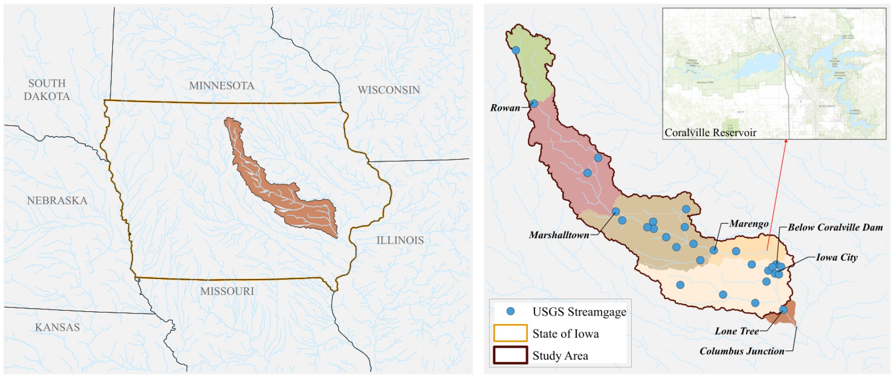
Figure 1. Iowa River Basin: locations of the USGS stream gauges and Coralville Reservoir.
Applsci 15 11656 g001
Figure 2. LSTM unit structure for the time step t to t + 1 .
Applsci 15 11656 g002
Figure 3. LSTM-based encoder–decoder model structure with t h time step input and t f time step output.
Applsci 15 11656 g003
Figure 4. LSTM-based encoder–decoder model for streamflow forecasting.
Applsci 15 11656 g004
Figure 5. LSTM-predicted streamflow vs. HEC-HMS-simulated streamflow at a 1-h lead time for the test dataset across models trained with datasets of varying sizes. The red dashed line represents the 1:1 line, indicating perfect agreement.
Applsci 15 11656 g005
Figure 6. LSTM-predicted streamflow vs. HEC-HMS-simulated streamflow at a 12-h lead time for the test dataset across models trained with datasets of varying sizes.
Applsci 15 11656 g006
Figure 7. Performance of LSTM models trained with different training set sizes across all lead times.
Applsci 15 11656 g007
Figure 8. Performance of LSTMs using PL and MSE loss functions on the test set at 1-h (left plots) and 12-h lead times (right plots). The upper plots correspond to PL with q = 0.8 , and the lower plots correspond to q = 0.9 . The red dashed line represents the 1:1 line, indicating perfect agreement.
Applsci 15 11656 g008
Figure 9. Performance of LSTM models using AP and MSE loss functions on the test set at two different lead times. The red dashed line represents the 1:1 line, indicating perfect agreement.
Applsci 15 11656 g009
Figure 10. Performance of LSTM models using different loss functions across various lead times.
Applsci 15 11656 g010
Figure 11. Time series of observed and forecasted rainfall (top plot) and forecast errors (bottom plot) from January to November 2020 at a 1-h lead time.
Applsci 15 11656 g011
Figure 12. Histograms of rainfall forecast errors and their fitted probability distributions for different rainfall categories at 1-h lead time. The categories, arranged from top to bottom, are no rainfall, light, moderate, heavy, and very heavy.
Applsci 15 11656 g012
Figure 13. Performance of PLSTM at 1-h and 12-h lead times. Each black dot represents the mean predicted streamflow from the PLSTM model plotted against the corresponding streamflow simulated by HEC-HMS. The red dashed line represents the 1:1 line, indicating perfect agreement.
Applsci 15 11656 g013
Figure 14. Comparison of streamflow time series from HEC-HMS simulations and PLSTM model predictions. The upper plot shows results at a 1-h lead time, while the bottom plot corresponds to a 12-h lead time.
Applsci 15 11656 g014
Table 1. Performance evaluation of the HEC-HMS model for the 8–28 June 2008 calibration event.
Gauge StationNSERSRPBIAS (%)NSE (Peak)RSR (Peak)PBIAS (Peak) (%)
Rowan0.900.30−1.720.570.60−1.40
Marshalltown0.730.505.510.630.645.51
Marengo0.870.404.230.750.533.50
Iowa City0.960.20−3.490.960.20−3.22
Lone Tree0.890.300.200.840.390.17
Table 2. Performance evaluation of the HEC-HMS model validated for the 26 April–14 May 2013 event.
Gauge StationNSERSRPBIAS (%)NSE (Peak)RSR (Peak)PBIAS (Peak) (%)
Rowan0.680.6−8.720.540.72−8.2
Marshalltown0.640.6−10.480.480.68−9.82
Marengo0.710.59.230.680.68.72
Iowa City0.910.4−5.360.900.4−4.95
Lone Tree0.620.66.300.470.785.64
Table 3. Performance of LSTMs with PL and MSE loss functions at different lead times.
Loss FunctionLead Time (Hour)NSENSE
( y i > 155 (cms))
PL (q = 0.8)10.960.14
PL (q = 0.9)10.980.82
MSE10.930.12
PL (q = 0.8)120.89−1.33
PL (q = 0.9)120.91−0.91
MSE120.88−0.90
Table 4. Performance of LSTM models using AP and MSE loss functions for varying lead times.
Loss FunctionLead Time (Hour)NSENSE ( y i > T )
AP10.970.76
PL (q = 0.9)10.980.82
MSE10.930.12
AP120.960.62
PL (q = 0.9)120.91−0.91
MSE120.88−0.90
Table 5. Performance metrics of the PLSTM model at different lead times.
Lead Time (Hours)NSEPICPMPIWCRPS
10.94510.995624.83582.2604
20.92890.995825.5742.3803
30.91820.995325.13132.5248
40.90030.993725.02922.7112
50.87900.992225.0572.9270
60.85570.990625.16363.1485
70.83250.988425.32853.3621
80.81020.986425.53473.5644
90.78930.984725.75263.7521
100.77040.983225.94513.9245
110.75320.980926.08164.0781
120.73520.978926.13114.2355
Disclaimer/Publisher’s Note: The statements, opinions and data contained in all publications are solely those of the individual author(s) and contributor(s) and not of MDPI and/or the editor(s). MDPI and/or the editor(s) disclaim responsibility for any injury to people or property resulting from any ideas, methods, instructions or products referred to in the content.