Validating Express Rail Optimization with AFC and Backcasting: A Bi-Level Operations–Assignment Model to Improve Speed and Accessibility Along the Gyeongin Corridor

Abstract

This study develops an integrated bi-level operations–assignment model to optimise express service on the Gyeongin Line, a core corridor connecting Seoul and Incheon. The upper level jointly selects express stops and time-of-day headways under coverage constraints—a minimum share of key stations and a maximum inter-stop spacing—while the lower level assigns passengers under user equilibrium using a generalised time function that incorporates in-vehicle time, 0.5× headway wait, walking and transfers, and crowding-sensitive dwell times. Undergrounding and alignment straightening are incorporated into segment run-time functions, enabling the co-design of infrastructure and operations. Using automatic-fare-collection-calibrated origin–destination matrices, seat-occupancy records, and station-area population grids, we evaluate five rail scenarios and one intermodal extension. The results indicate substantial system-wide gains: peak average door-to-door times fall by approximately 44–46% in the AM (07:00–09:00) and 30–38% in the PM (17:30–19:30) for rail-only options, and by up to 55% with the intermodal extension. Kernel density estimation (KDE) and cumulative distribution function (CDF) analyses show a leftward shift and tail compression (median −8.7 min; 90th percentile (P90) −11.2 min; ≤45 min share: 0.0% → 47.2%; ≤60 min: 59.7% → 87.9%). The 45-min isochrone expands by ≈12% (an additional 0.21 million residents), while the 60-min reach newly covers Incheon Jung-gu and Songdo. Backcasting against observed express/local ratios yields deviations near the ±10% band (PM one comparator within and one slightly above), and the Kolmogorov–Smirnov (KS) statistic and Mann–Whitney (MW) test results confirm significant post-implementation shifts. The most cost-effective near-term package combines mixed stopping with modest alignment and capacity upgrades and time-differentiated headways; the intermodal express–transfer scheme offers a feasible long-term upper bound. The methodology is fully transparent through provision of pseudocode, explicit convergence criteria, and all hyperparameter settings. We also report SDG-aligned indicators—traction energy and CO₂-equivalent (CO₂-eq) per passenger-kilometre, and jobs reachable within 45- and 60-min isochrones—providing indicative yet robust evidence consistent with SDG 9, 11, and 13.

1. Introduction

Urban rail systems are central to metropolitan mobility, yet the door-to-door performance experienced by passengers often falls short of nominal rolling-stock capabilities. This is because, beyond vehicle speed, stopping strategy, time-of-day headways, and geometric or capacity constraints collectively shape effective service quality, accessibility, and network stability. Coordinating these levers in the design of express services thus presents a core challenge at the intersection of operations research and transport economics.

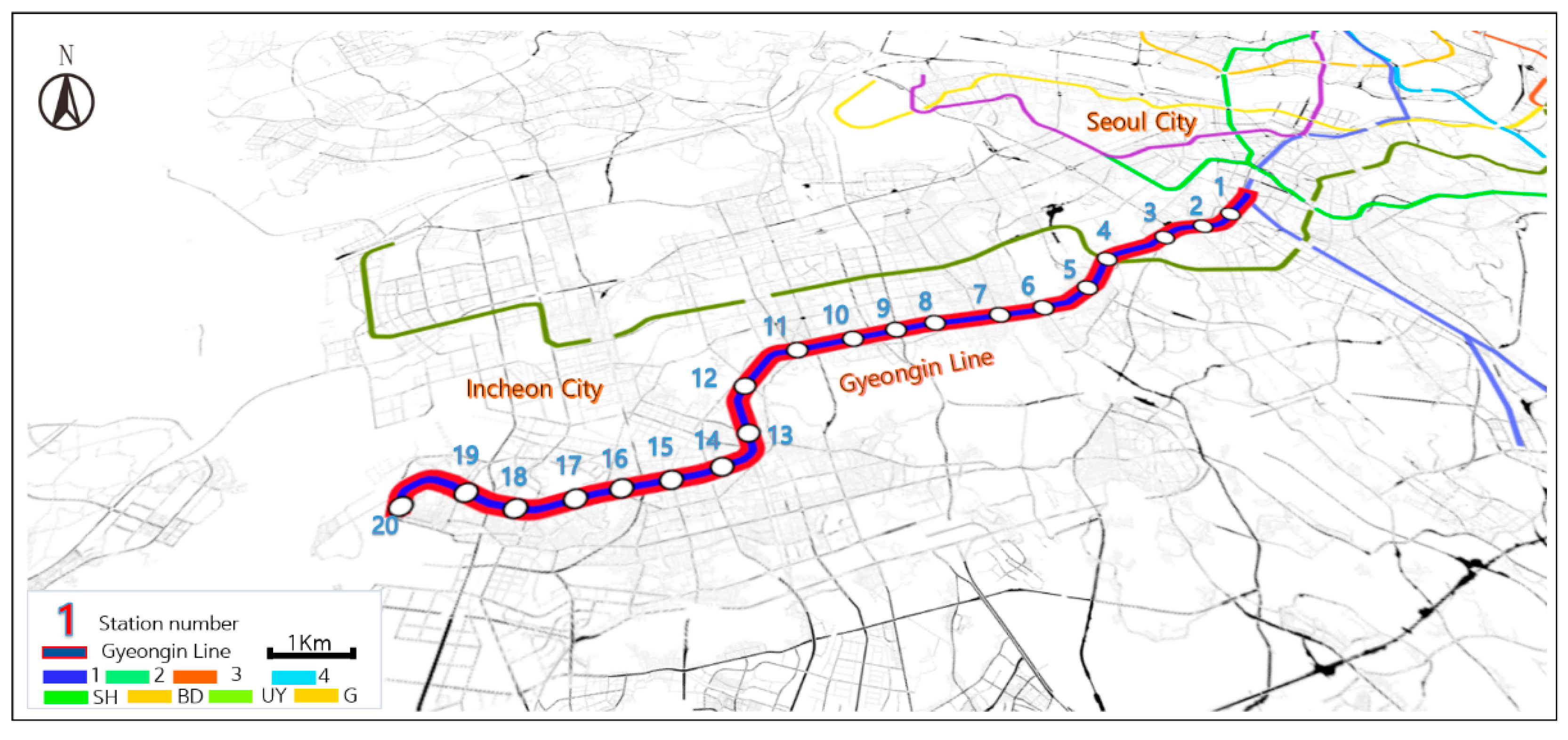
Within this broader context, the Seoul–Incheon megaregion is home to nearly half the national population and exhibits intense core–periphery commuting flows. The Gyeongin Line, built in 1897 and long since transformed from a freight corridor into the principal passenger spine between Seoul (national core) and Incheon (port/logistics hub and expanding employment centre), remains largely at-grade, generating cumulative externalities such as severed streets and noise and offering limited overtaking opportunities. Under these circumstances, the corridor’s door-to-door performance averages approximately 29.3 km/h despite nominal subway top speeds of 70–90 km/h, indicating structural bottlenecks in stopping patterns and headway design. Figure 1 offers spatial context by illustrating the corridor and the key interchanges that motivate the express-service problem studied herein.

Prior studies have primarily optimised either operations (stops/headways) or passenger assignment in isolation and seldom co-designed them with corridor-level infrastructure options. Replication has been further hindered by corridor-specific formulations and the limited disclosure of calibration and solution details. To address these limitations, we (i) propose a compact bi-level operations–assignment model that jointly selects express stops and time-differentiated headways at the upper level while assigning passengers under user equilibrium with crowding-sensitive dwell times at the lower level; (ii) provide a corridor-agnostic parameterisation workflow based on automatic fare collection (AFC), operational performance statistics (OPS), and General Transit Feed Specification (GTFS) data structures, including segment-wise congestion estimation using the Bureau of Public Roads (BPR) function and dwell-time calibration; (iii) ensure reproducibility through step-by-step pseudocode, explicit convergence criteria, and full hyperparameter settings; and (iv) evaluate realistic policy packages, namely operations-only, infrastructure-enabled, and an intermodal extension, on the Gyeongin corridor.

Building on this framing, we define the problem as one of aligning stopping policies and time-of-day headways with corridor geometry and capacity under minimum-coverage and spacing constraints. The resulting framework supports scenario analysis and genuine sensitivity tests to quantify trade-offs among travel time, accessibility, and operational stability while also clarifying near-term and long-term implementation pathways.

In addition to efficiency and accessibility, we map the evaluated packages to Sustainable Development Goals (SDGs) 9, 11, and 13 by reporting traction-energy and CO₂ intensity (per passenger-kilometre), alongside employment accessibility within 45/60 min isochrones; these isochrones serve as indicative yet robust sustainability metrics, as elaborated in the Discussion.

Building on these objectives, we re-optimise the existing express service rather than introducing a new one and test how underground alignment improvements could enable a faster and more reliable express service under mixed operations. To this end, we develop a bi-level operations–assignment framework that integrates operational policies, namely stopping patterns and time-of-day headways, with infrastructure conditions such as undergrounding and alignment straightening. In this framework, the upper level selects station stops and headways subject to safety and coverage constraints, while the lower level performs passenger assignment under user-equilibrium conditions based on generalised travel time, thereby capturing the interaction between operating decisions and traveller behaviour. To reflect corridor-specific constraints, alternative track and station design schemes from the Gyeongin undergrounding initiative are parameterised and incorporated into segment run-time and dwell-time functions. Simulation experiments are then conducted to quantify how each construction scenario alters the performance of the existing express service, both in isolation and in combination with timetable redesign, relative to an all-stop baseline.

This dual focus enables simultaneous evaluation of infrastructure improvements and operational optimisation, offering insights to enhance both service quality and system efficiency. Accordingly, the model and results presented herein are expected to inform policy decisions related to station-area redevelopment and the broader modernisation of the Seoul metropolitan transport system [1].

Building on this modelling foundation, the proposed bi-level mixed optimisation for the Gyeongin Line is based on Wardrop’s first principle, a user-equilibrium (UE) approach widely applied in public transport planning [2]. In the lower-level problem, passenger route choice is modelled using UE and stochastic UE (SUE) assignment algorithms [3]. Meanwhile, in the upper-level problem, the set of express stops and headways is determined via mixed-integer optimisation to minimise total generalised cost. To capture model realism, the endogeneity of dwell time and the BPR-type congestion cost function, often oversimplified in previous studies, are calibrated using AFC-based seat occupancy records and regression analysis [4].

The research process comprises four stages: (1) a systematic review of prior studies and policy reports; (2) empirical data collection on station-level demand, boarding and alighting patterns, and seat occupancy; (3) model formulation and solution design; and (4) scenario-based simulation and validation. Building on this framework, five operating scenarios are evaluated: full-stop service, limited-stop express, undergrounding with alignment improvements, headway adjustment, and mixed operation, along with an additional scenario involving bus–rail transfer integration.

Figure 2 shows the station locations along the Gyeongin Line and the numbering scheme used throughout the analysis.

The results suggest that average travel time during peak AM/PM periods is reduced by over 40%. Furthermore, sensitivity tests for key constraints—including the critical-station ratio, maximum stop spacing, and headway—yield deviations within ±10%, confirming the model’s robustness and validity. Overall, by jointly considering operational policies and infrastructure conditions, the study offers a quantitative assessment of both efficiency and equity in express service design, providing actionable evidence to improve service quality and guide metropolitan rail policy in the Seoul Capital Region.

2. Materials and Methods

2.1. Review of Previous Studies

Research on urban-rail express services spans four thematic strands that collectively shape door-to-door performance: (i) schedule-based demand assignment and UE under path overlap; (ii) skip-stop and express service design with headway control and meet–overtake constraints; (iii) reliability-aware timetabling and dwell–transfer processes; and (iv) welfare and accessibility appraisal beyond mean travel time. By similarly following these strands, we position the present study within the broader literature while maintaining corridor-agnostic notation consistent with Section 2.2, Section 2.3 and Section 2.4.

Urban-rail express configurations pose a system-design problem: where trains should stop, how frequently they should run, and how meets–overtakes and transfers should be organised so that door-to-door generalised time is minimised without violating coverage, capacity, and safety constraints. These decisions alter costs in non-linear ways—through headway-induced waiting, transfer penalties, crowding-sensitive dwell times, and node throughput—and traveller choices, in turn, feed back into loads and reliability. Consequently, modelling is required to (i) represent generalised costs and operational constraints with fidelity, (ii) predict equilibrium passenger flows under altered stopping and headway patterns, and (iii) optimise the coupled operator–user system so that efficiency gains do not compromise accessibility or robustness [5,6,7,8,9,10,11].

On the demand side, research has evolved from frequency-based ‘optimal-strategy’ assignment to schedule-based formulations that account for departures and arrivals, in-station walking, and the expected 0.5 × headway wait within a consistent utility framework [7,12]. In particular, issues of path overlap and correlation have been addressed using path-size and similarity corrections, alongside sampling–estimation techniques, to prevent probability inflation for overlapping routes [13,14,15,16].

Meanwhile, on the supply side, research has advanced from heuristic skip–stop rules to bi-level and multi-objective optimisation frameworks, wherein the upper level minimises generalised passenger cost or maximises welfare, while the lower level enforces SUE assignment subject to capacity, platform, and meet/overtake constraints [17]. A consistent finding of this research is that, when crowding disutility, transfer penalties, and node constraints are modelled appropriately, coordinated express and all-stop operations, combining skip–stop patterns with tuned headways—reduce system generalised cost without requiring physical expansion. However, if interchange throughput is neglected, crowding may simply shift from trains to hubs [18,19]. Beyond throughput considerations, reliability constraints further reshape optimal design: even small dwell-time extensions disrupt train spacing, reduce capacity, and intensify downstream delays. These effects underscore the need for robust timetabling and the joint adjustment of meet/overtake patterns with time-of-day headways [9]. To support such design choices, train–passenger coupling through the microscopic urban rail relationship links flow, density, and speed, enabling quasi-dynamic evaluation of frequency and overtake strategies during peak periods [20].

In practice, three-level performance–timetable frameworks and robust railway planning surveys establish consistent links between macro-scale key performance indicators (KPIs) and micro-scale timetables [21,22]. Quantifying accessibility improvements via isochrone expansion [23,24]. In parallel, scenario-robust timetabling under demand uncertainty has received growing attention [25]. Empirical analyses of arrival and waiting processes and door-to-door travel-time variability demonstrate that policy appraisals must account for full distributions and variance components rather than mean values alone [26,27,28,29]. Complementing this distributional view, the provision of personalised predictive crowding information can shift route choices and enhance system-level welfare through endogenous load rebalancing [30].

From a service-design perspective, coordinated optimisation of skip–stop patterns with headways and overtakes has become increasingly prevalent. Specifically, genetic-algorithm methods, passenger-adapted skip–stop plans, and learning-based policies (e.g., Q-learning) coupling inflow control with rescheduling all report simultaneous gains in average travel time and reliability when node and platform constraints are explicitly modelled [31,32,33]. However, rule-based skip–stop operations are not invariably Pareto-improving, as neglecting node and dwell constraints can misrepresent the associated benefits [34].

With respect to passenger behaviour and welfare, previous estimates indicate that crowding substantially increases the marginal disutility of in-vehicle time as standee density rises. Moreover, the elasticity of dwell time with respect to boarding and alighting volumes feeds back into the reliability boundary and shapes the feasible set of optimal solutions [35,36,37,38]. Building on this behavioural foundation, comparative studies from the Tokyo metropolitan area find that, when path correlation and flow dependence are explicitly modelled, probit SUE and enhanced logit models yield more robust performance in both fit and behavioural extrapolation [39]. On the policy side, consumer-surplus frameworks institutionalise the linkage between speed improvements and welfare assessment [16,40,41].

In Korea, the tradition of mixed all-stop–express operations and the multi-line interchange topology of the Seoul Capital Region (e.g., Onsu–Line 7, Sosa–Seohae, Bupyeong–Incheon Line 1) make the Gyeongin corridor an effective test bed for (i) evaluating jointly designed stopping-pattern and time-of-day headway policies under realistic interchange and reliability constraints, (ii) validating a schedule-based UE assignment using AFC-derived origin–destination (OD) matrices against observed operations, and (iii) quantifying accessibility improvements via isochrone expansion. Findings from this corridor suggest that skip–stop strategies can reduce system-wide travel times without new infrastructure. However, the realised benefits depend on the waiting-time share and OD structure, underscoring the need to co-optimise express patterns with headway settings and coverage thresholds [42].

Although numerous studies have examined assignment and express design separately, few have co-designed stopping patterns and time-of-day headways while endogenising dwell and segment-level congestion or have maintained a corridor-agnostic formulation suitable for replication. These limitations are compounded by corridor-specific notation and insufficient disclosure of calibration procedures and solver settings. To address these gaps, the present study (i) formulates a compact bi-level operations–assignment model with explicit coverage–spacing constraints; (ii) calibrates dwell (α,β) and segment BPR parameters {λ_s, θ_s} using AFC/OPS evidence; (iii) embeds undergrounding and realignment directly into run-time functions rather than applying ex-post deductions; and (iv) ensures reproducibility through pseudocode, convergence criteria, and full disclosure of hyperparameters. Together, these steps position this research at the intersection of express-service planning, reliability-aware assignment, and corridor-scale accessibility appraisal.

2.2. Key Assumptions and Mathematical Formulation for Model Development

2.2.1. UE Optimisation Assumptions

The express service demand-assignment model developed in this study rests on several fundamental assumptions designed to capture both the temporal variability of peak-period demand across the metropolitan network and the effects of track realignment resulting from underground construction.

First, the model assumes that UE, as defined by Wardrop’s first principle, holds across the entire network. In other words, passengers are assumed to choose the route that minimises their individual generalised travel cost for a given OD pair, such that under equilibrium conditions, all used paths for that pair exhibit equal generalised costs. This assumption aligns with previous findings from Japanese and global studies (e.g., those using probit-based SUE models), which confirm that decentralised rational route choice persists even under peak-hour congestion.

Second, the components of generalised travel cost are explicitly defined. In particular, the generalised cost is decomposed into (i) platform waiting time, (ii) in-vehicle travel time, and (iii) transfer and crowding disutility. Infrastructure improvements such as undergrounding and horizontal realignment are modelled as directly affecting in-vehicle travel time. In contrast, timetable decisions, such as changes to headways or stopping patterns, are reflected as variations in platform waiting time and crowding-related disutility.

Third, express stop–selection constraints are embedded in the optimisation. Accordingly, at least a fraction K of key stations must be served by express trains, and the maximum spacing between consecutive express stops is limited to 12 km. These constraints formalise equity and coverage requirements commonly adopted in practice.

Finally, the endogeneity of station dwell times is explicitly accounted for in the model. Station-specific boarding and transfer volumes determine dwell times, which in turn influence train running times and headways. Accordingly, dwell times are modelled as a function calibrated based on AFC and field-observed data, ensuring that the feedback loop between passenger inflows, dwell durations, and service reliability is reliably captured.

Based on these assumptions, the model is mathematically formulated as follows:

(1)

Objective Function (minimisation of total generalised cost):

$$\min \mathrm{Z}={\sum }_{\mathrm{s}\in \mathrm{S}}{\sum }_{\mathrm{a}\in \mathrm{A}}{\sum }_{\mathrm{k}\in {\mathrm{K}}_{\mathrm{sa}}}{{\mathrm{f}}_{\mathrm{sa}}}^{\mathrm{k}}·{{\mathrm{C}}_{\mathrm{sa}}}^{\mathrm{k}},$$

(i)

where ${f_{sa}}^k$ represents the flow assigned to path k for (o,d) pair (s,a), and ${C_{sa}}^k$ denotes the corresponding generalised path cost.

(ii)

Equilibrium Condition (Wardrop’s first principle):

$${{\mathrm{f}}_{\mathrm{sa}}}^{\mathrm{k}}蠧0\Rightarrow {{\mathrm{C}}_{\mathrm{sa}}}^{\mathrm{k}}={{\mathrm{C}}_{\mathrm{sa}}}^{\min },{{\mathrm{f}}_{\mathrm{sa}}}^{\mathrm{k}}=0\Rightarrow {{\mathrm{C}}_{\mathrm{sa}}}^{\mathrm{k}}\ge {{\mathrm{C}}_{\mathrm{sa}}}^{\min }\sum k\in k_{sa}$$

(2)

This ensures that, at equilibrium, all utilised paths for each OD pair have an equal generalised cost, while unused paths cannot have a lower cost.

(iii)

Constraints:

K ≥ K_min (minimum proportion of the demand served by express stops)

d ≤ 12,000 m (maximum distance between successive express stops)

Additional operational constraints are also imposed on feasible headways and stopping patterns to ensure realistic service plans.

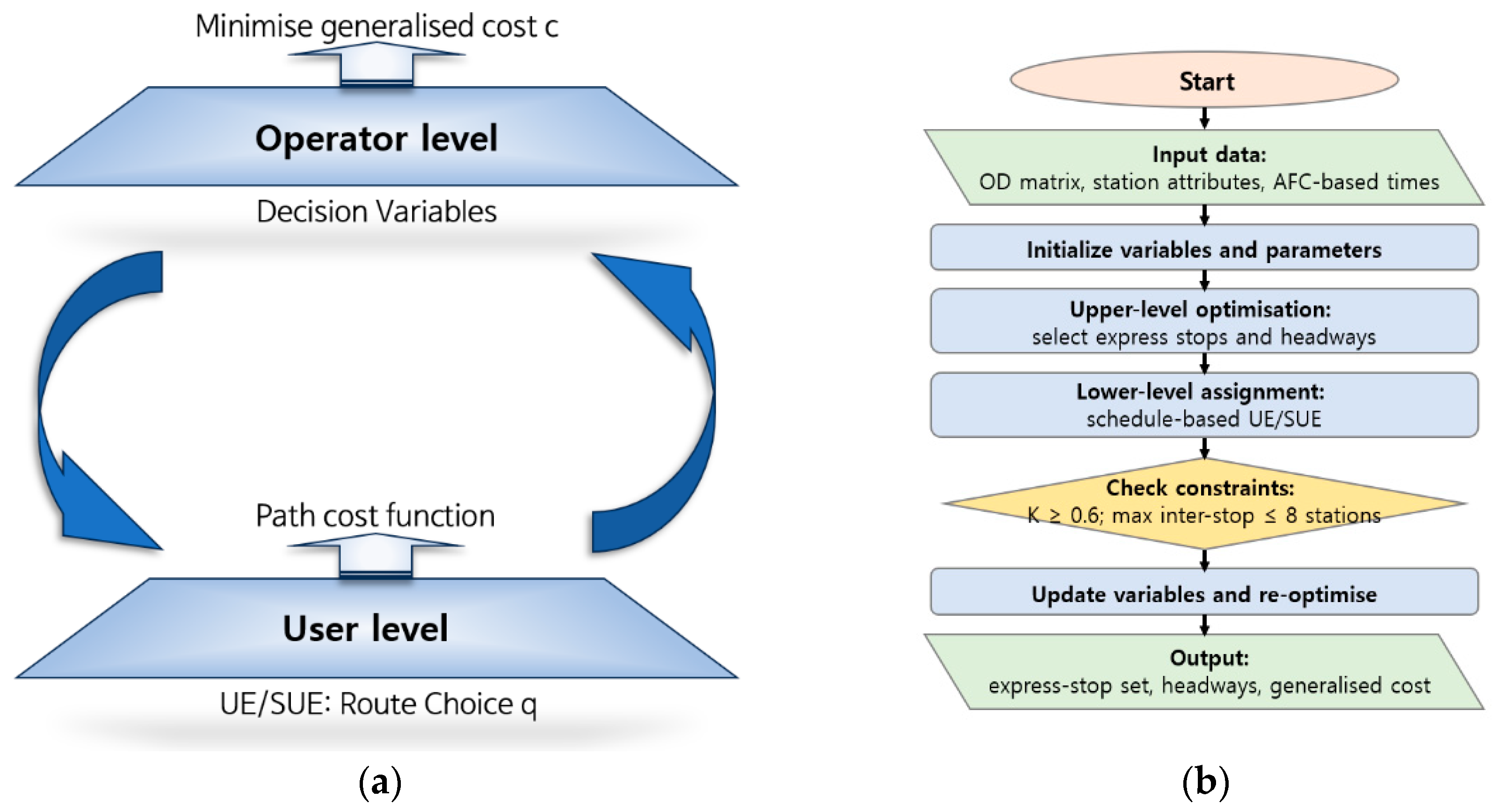
This integrated formulation combines the theoretical foundations of UE/SUE assignment, skip–stop optimisation, and congestion feedback models while explicitly incorporating infrastructure improvements, such as undergrounding, into the travel time function (Figure 3).

Consequently, the overall problem is formulated as a bi-level optimisation model:

• Upper-Level Problem (operator’s decision):

• The operator selects the stopping pattern x and headway H to minimise the total generalised cost Z(x, H), which is computed endogenously from the lower-level solution. The optimisation is subject to constraints on the minimum coverage ratio, maximum inter-stop spacing, and allowable headway bounds. Candidate solutions are evaluated using metaheuristic techniques, such as genetic algorithms or simulated annealing, with the lower-level problem solved iteratively for each case.

• Lower-Level Problem (user equilibrium assignment):

• For a given (x, H) configuration, passengers choose routes based on UE principles until a stable demand distribution is attained. Convergence is deemed achieved when the cost difference between any utilised path ${C_{sa}}^k$ and the minimum-cost path ${C_{sa}}^{min}$ for the same OD pair falls below a defined threshold.

$$\begin{array}{c}min\\ H,y\end{array}Z\left(H,y\right)=\sum _{s,a}\sum _{k\in k_{sa}}{f}_{sa}^k\left(x\right)c_{sa}^k\left(x;H,y\right)s.t.xsovlves;K\ge K_{min},D_{max},H\in \mathrm{H}$$

(3)

The solution approach adopted in the present study is based on an iterative metaheuristic framework. In the initial stage, a randomised set of candidate stopping patterns and headway schedules is generated. For each candidate, the lower-level problem is solved to obtain the UE flow distribution and compute the total generalised cost. The objective function for each candidate is then evaluated in the upper-level problem, and new solutions are generated using heuristic search operators. This process is repeated until the convergence criteria are met, when either the improvement in the objective function falls below a specified tolerance or the maximum number of iterations is reached.

This iterative approach not only integrates UE and SUE traffic assignment, skip–stop optimisation, and congestion feedback models, as highlighted in previous studies, but also introduces a key methodological distinction. Japanese studies have emphasised route overlap and in-vehicle congestion effects, while international studies have developed skip–stop optimisation frameworks. In contrast, the present research incorporates infrastructure improvements, such as undergrounding and track realignment, directly into the in-vehicle travel time function. By jointly considering operational policies and infrastructure conditions, this study establishes a novel integrated optimisation framework that extends the scope of existing models.

2.2.2. Key Variables Related to Urban Railway Operations

The operational variables of the model comprise the headway (H), stopping pattern (x), dwell-time function, and section-specific running-speed and congestion coefficients. Specifically, the headway is initially set to 5 min during peak hours and 8 min during off-peak hours and is subsequently varied within a ±10% range in the sensitivity analysis to examine its marginal effects on total generalised cost and platform congestion [43,44].

Meanwhile, the stopping pattern is represented by a binary decision variable xi ∈ {0,1}, which indicates whether an express train stops at station i and is determined in the upper-level optimisation problem.

The dwell-time function is formulated as j = αN_j + β, where N_j denotes the boarding demand at station j. Parameters $\alpha$ and $\beta$ are estimated via regression analysis using AFC data and in-train seat occupancy records (R² = 0.87), reflecting the non-linear increase in dwell time under conditions of low seat availability.

Additionally, section-specific running speeds and congestion factors are parameterised to allow infrastructure improvements, such as undergrounding, track realignment, and increases in curve radius, to directly affect the in-vehicle travel time function.

The infrastructure-related variables employed in this study are summarised in

Table 1. Data schema and aggregation used in parameterisation ¹.

Stream	Key Fields	Time Window and Binning	Use in Model
AFC (Smart card)	Card ID, tap time, tap station, direction, product type	Weekday peaks 07:00–09:00/17:30–19:30; 5- and 15-min bins	OD inference; platform accumulation; demand scaling
OPS (Operational logs)	Train ID, actual departure/arrival times, dwell, headway, seat occupancy	Synchronized to AFC bins; missingness flagged	Dwell calibration; validation
GTFS (Network)	Stop sequence, scheduled run times, transfer links, segment length and geometry	Service calendar; corridor topology	Lower-level costs; network build

¹ Personally identifying fields are anonymised. All times are localised to UTC + 9. Sparse stations are flagged and excluded from calibration where appropriate.

, derived from reports by the Incheon Research Institute (2019) [3]. To operationalise these proposals within the model, we translate them into quantitative variables, such as segment length, curve radius, depth, and construction method, for use as model inputs.

2.2.3. Characteristics of the Demand Assignment Theory for Express Operations

The express demand assignment problem addressed in this study extends beyond merely reducing the number of intermediate stops compared with ordinary trains; it also accounts for UE conditions, public service coverage constraints, and the endogenous relationship between dwell times and congestion. These features are discussed in detail below.

First, path consistency and selective stopping are explicitly considered. The express service operates along the same physical corridor as the ordinary line, with the only distinction being its stopping pattern. Consequently, passengers with the same OD pair select between the ordinary and express services by minimising their generalised cost, formalised under the Wardrop UE condition. This implies that express service design does not constitute an independent line-planning problem but rather a multi-layered equilibrium allocation problem within a shared corridor.

Second, public-service constraints are formally specified. While previous studies have relied on qualitative rules such as ‘all major transfer stations must be served’, this study introduces quantifiable constraints, including a coverage ratio (K ≥ K_min) and an upper limit on station spacing (≤12 km). This enables explicit incorporation of the trade-off between system efficiency (i.e., minimisation of total generalised cost) and service equity (i.e., guaranteed accessibility).

Third, the model accounts for the endogeneity of dwell times and congestion. During peak hours, station layout influences the spatial distribution of congestion, which lengthens dwell times and propagates delays through headway adjustments and passenger queues. The number and location of express stops not only affect operating efficiency but also interact with equilibrium passenger flows. To reflect this mechanism, the dwell-time function is embedded in the model and calibrated using AFC records and field observations.

Fourth, international comparability is prioritised. The parallel operation of express and local services, exemplified by Tokyo’s JR Chūō Line Rapid and express–local combinations in US BRT networks, has long demonstrated the effectiveness of prioritising major nodes and limiting maximum station spacing. The constraint set adopted in this study mathematically reflects international best practices.

• Based on these premises, the station importance score (S_i) detailed in Table 6 is calculated as the weighted sum of three factors: the peak two-hour boarding–alighting total (D_i), temporal balance index (B_i, 0–1), and annual scaling factor (R_i).

$${\mathrm{B}}_{\mathrm{i}}=1-{\displaystyle \frac{\left|{\mathrm{A}\mathrm{M}}_{\mathrm{i}}-{\mathrm{P}\mathrm{M}}_{\mathrm{i}}\right|}{{\mathrm{A}\mathrm{M}}_{\mathrm{i}}+{\mathrm{P}\mathrm{M}}_{\mathrm{i}}}},$$

(4)

where D_i denotes the normalised peak two-hour demand (AM + PM, Table 4, peak total), and B_i represents the symmetry of AM–PM demand, with values closer to one indicating more balanced flows.

• To integrate indicators with differing scales and units, linear normalisation is applied, as expressed in Equation (5):

$${{{\mathrm{D}}_{\mathrm{i}}}^{\mathrm{*}}={\displaystyle \frac{{\mathrm{D}}_{\mathrm{i}}-\mathrm{m}\mathrm{i}\mathrm{n}\left(\mathrm{D}\right)}{\mathrm{m}\mathrm{a}\mathrm{x}\left(\mathrm{D}\right)-\mathrm{m}\mathrm{i}\mathrm{n}\left(\mathrm{D}\right)}}, {{\mathrm{R}}_{\mathrm{i}}}^{\mathrm{*}}={\displaystyle \frac{{\mathrm{R}}_{\mathrm{i}}- \mathrm{m}\mathrm{i}\mathrm{n}\left(\mathrm{R}\right)}{\mathrm{m}\mathrm{a}\mathrm{x}\left(\mathrm{R}\right)-\mathrm{m}\mathrm{i}\mathrm{n}\left(\mathrm{R}\right)}}}_{\mathrm{i}}$$

(5)

• At the station importance score evaluation stage, the weighted sum is calculated as follows:

$${\mathrm{S}}_{\mathrm{i}}=\mathsf{\alpha }{{\mathrm{D}}_{\mathrm{i}}}^{\mathrm{*}}+\mathsf{\beta }{{\mathrm{B}}_{\mathrm{i}}}^{\mathrm{*}}+\mathsf{\gamma }{{\mathrm{R}}_{\mathrm{i}}}^{\mathrm{*}}, \mathsf{\alpha }+\mathsf{\beta }+\mathsf{\gamma } =1,$$

(6)

where D_i^* is the normalised peak two-hour demand, B_i^* is the temporal balance index, and R_i^* is the annual scaling factor.

The baseline weights are set to α = 0.70, β = 0.20, and γ = 0.10, indicating that the normalised demand D_i^* serves as the primary criterion, while B_i^* and R_i^* adjust for time-of-day imbalance and annual representativeness, respectively.

A sensitivity analysis with a variation of ±0.05 in each weight is reported in Table 1, confirming the stability of the ranking results.

• Based on this scoring, stations are then sorted in descending order of S_i, and the coverage ratio is calculated using actual demand D_i rather than S_i:

$$\left(\mathrm{k}\right)={\displaystyle \frac{\sum \mathrm{i}\in \mathrm{\top }-\mathrm{k} {\mathrm{D}}_{\mathrm{i}}}{\sum \mathrm{i} {\mathrm{D}}_{\mathrm{i}}}},$$

(7)

where k is the number of top-ranked stations considered. The express stop set is finalised when two constraints are satisfied: (i) coverage K ≥ K_min (with K = 0.6 in this study) and (ii) maximum spacing ≤ 8 stations along the corridor. The spacing constraint is checked using interstation adjacency on a line graph.

These constraints are not arbitrarily defined but are grounded in established guidelines and empirical evidence. The Ministry of Land, Infrastructure and Transport (MOLIT) mandates in its metropolitan railway service-level guidelines that express services must cover more than 60% of major nodes to satisfy public accessibility criteria. An analysis of AM–PM peak AFC data confirms that the top eight stations account for 60% coverage, thereby validating K = 0.6 as a balanced point between efficiency and equity. The maximum spacing constraint (≤8 stations) aligns with international precedents, including JR Chūō Rapid and Keiyō Line Limited Express, where stop spacing seldom exceeds this level.

A sensitivity experiment is also conducted using K = 0.7 and a spacing limit of ≤10 stations. Increasing K improves service coverage but slightly raises average travel times, whereas loosening the spacing constraint shortens travel times but reduces accessibility in certain low-demand segments, together illustrating the efficiency–equity trade-off.

Dwell time is estimated using OPS combined with AFC-based platform accumulation data collected during the AM and PM peak windows (07:00–09:00; 17:30–19:30). Based on these data, the preferred specification is a linear model incorporating passenger load N_j and an optional variability term, estimated from more than 300 dwell-time observations obtained from Seoul Metro during the two-hour peak periods, yielding:

$${\mathrm{t}}_{\mathrm{d}\mathrm{w}\mathrm{j}}=0.0061{\mathrm{N}}_{\mathrm{j}} + 0.42 ({\mathrm{R}}^2=0.87),$$

(8)

as reported in the current manuscript (Equation (8)). For transparency, the complete regression specification, including variables, link function, sample size, time window, and diagnostics (R², mean absolute error (MAE), and 95% confidence intervals for α and β), is also provided. To further ensure robustness, a standard winsorization is applied at the 1st and 99th percentiles of t_dwell to reduce the influence of rare saturation events (platform spillback); the corresponding unadjusted results are presented in

Table 2. Corridor-specific mapping of generic symbols to Gyeongin values.

Stream	Meaning	Default/Prior Range	Gyeongin Value (Estimated or Policy)	Source/Method
$t_{0,s}$	Free-run time of segment s	GTFS schedule ± tolerance	None	GTFS/OPS alignment
$c_S$	Capacity of segment s	trains/h	None	OPS/platform rules
${\lambda }_s,{\theta }_s$	BPR parameters (segment-wise)	$\lambda \mathrm{ϵ}\left[0.05,0.30\right],$ $\theta \mathrm{ϵ}[2.5,5.0]$	$[{\widehat{\lambda }}_s,{\widehat{\theta }}_s\pm CI$]	Nonlinear least squares
$a,\beta ,\left(r\right)$	Dwell coefficients (load, variance)	$\mathrm{Signs}\alpha >0,\beta >0$	$[\widehat{a},\widehat{\beta },\left(\widehat{\gamma }\right)\pm CI]$	OLS/GLS on OPS × AFC
${\delta }_{cov}$	Minimum coverage threshold	[0.6–0.9] of key stations	K ≥ 0.6	Policy rule/sensitivity
${\Delta }_{max}$	Maximum inter-stop spacing	By stations or distance cap	≤8 stations	Best practice + sensitivity

. At very high passenger loads, an upper cap equal to the 99th-percentile dwell observed is imposed to maintain numerical stability of the lower-level assignment while preserving the slope at typical loads. Finally, the complete set of coefficient estimates and confidence intervals is listed in Table 1. Further, in Equation (8), N_j denotes the number of boardings per 2 h peak at station j, and t_dw is the mean dwell time (min); the intercept (0.42 min) reflects base dwell time, while the slope quantifies marginal delay per additional passenger.

Equation (9), as presented below, initially used typical BPR constants (λ ≈ 0.15, θ ≈ 3.5–5.0) as default values. However, the revised formulation replaces corridor-wide constants with segment-specific estimates {λ_s, θ_s} while retaining t_0,s and c_0,s for each segment. For each segment s, speed–throughput pairs are constructed by aligning OPS run times with AFC-derived flows at screenlines, and the BPR function is calibrated by minimising error.

$$\mathrm{C} = {\mathrm{t}}_0 [1+\mathsf{\lambda }\frac{\mathrm{V}}{{(\mathrm{C}}_0{)}^{\mathsf{\theta }}}],$$

(9)

where t₀ is the free-flow travel time, V is the realised flow volume, C₀ is the link capacity, λ is the congestion sensitivity parameter (commonly set to 0.15), and θ is the exponent that captures the nonlinear rise in delay under heavy loading.

Rather than fixing the congestion parameters in Equation (9) to typical constants, estimating them for each segment captures spatial heterogeneity. Segment-level parameters are then fitted through nonlinear least squares using observed travel times and screenline throughputs from OPS and AFC, subject to mild regularity conditions (positivity and monotonicity). For transparency, we report R², RMSE, MAE, and 95% confidence intervals for each segment’s estimated parameters. The complete results are presented in Table 1, while the main text retains Equation (9) in its generic, corridor-agnostic form. As a diagnostic, we compare the model’s implied volume–delay curves with observed queueing patterns in operational logs, confirming that corridor-level backcasting remains within the ±10% band. Sensitivity to capacity assumptions is assessed by varying C₀ in Equation (9) by ±5–10%, as detailed in Table 2.

2.3. Solution Algorithm and Simulation Design

The express demand–assignment problem is structured as a bi-level formulation involving operator and user decision layers. At the upper level, the operator determines stopping patterns and headways across time periods, subject to safety and coverage constraints. At the lower level, travellers select routes under UE conditions. As closed-form solutions are rarely feasible for such problems, the formulation is cast as a variational inequality (VI) or mixed complementarity problem. We solve it using an iterative metaheuristic that alternates upper-level search with lower-level schedule-based assignment.

The empirical application focuses on the Dowon–Gaebong corridor of the Gyeongin Line. The analysis covers the AM peak (07:00–09:00) and PM peak (17:30–19:30) periods. Demand inputs consist of AFC-calibrated OD matrices combined with train seat-occupancy records, enabling consistent representation of station inflows, boarding and alighting profiles, and in-vehicle crowding.

We evaluate six operating scenarios: (S1) an all-stop baseline; (S2) a stand-alone limited-stop express on the surface alignment with baseline headways; (S3) a limited-stop express with undergrounding and realignment, where segment run times are replaced by those implied by the redesigned vertical and horizontal profile, and headways are held fixed to isolate infrastructure effects; (S4) a limited-stop express with time-of-day headway retuning on the surface alignment; (S5) an integrated rail operation in which all-stop and express services operate concurrently with passenger transfer allowed between them; and (S6) an intermodal extension of S5 that incorporates free-transfer express buses. Scenario S6 is included as a forward-looking exploratory upper bound to gauge multimodal potential; however, its near-term operability depends on the provision of dedicated bus priority, integrated fare and transfer systems, and coordinated stop-area organisation. Accordingly, S6 is excluded from ratio-based backcasting owing to the absence of an observed in-vehicle comparator but is retained in KPI and sensitivity analyses to illustrate directional benefits under supportive institutional conditions.

Performance is evaluated primarily in terms of total generalised cost, supplemented by average waiting time, average in-vehicle time, transfer-area crowding, dwell-time uplift, and the service-coverage ratio. The sensitivity analysis varies the share of key stations K, maximum inter-stop limit (measured in distance or number of stations), and headway H to assess parameter impacts on user welfare and operating efficiency, as well as to evaluate policy robustness.

Model validation is carried out on three fronts. First, results are compared with those of prior studies, particularly those on skip–stop applications, to confirm interpretative consistency with existing literature. Second, backcasting is conducted against observed operations to verify that the model replicates average travel times and crowding patterns with acceptable fidelity. Notably, the model uses a broader door-to-door denominator than the in-vehicle scheduled times used in observations. Third, sensitivity experiments on key variables are used to test the stability of outcome indicators, thereby establishing the robustness and practical applicability of the proposed framework.

2.3.1. Data Structure and Parameterization Workflow

Three operational data sources are integrated to support model parameterisation and validation. AFC records provide time-stamped entries and exits, from which OD flows are inferred. OPS supply realised departures and arrivals, platform assignments, headways, and dwell times, along with periodic seat-occupancy snapshots. GTFS timetables and the corridor network define stop sequences, scheduled run times, transfer links, and segment geometry.

Table 3. Scenario design matrix.

Scenario	Stopping	Headway	Alignment	Dwell/Cong	Rationale
S1 Baseline	All-stop	Baseline timetable	Surface (observed)	Calibrated dwell; calibrated BPR (segment-wise)	Benchmark for door-to-door costs and express/local shares under current practice.
S2 Limited-stop	Express stops only	Baseline timetable	Surface (observed)	Same as S1	Isolates pure stopping-pattern effects without changing frequency or geometry
S3 Express-alone	Express stops (as S2)	Fixed headways (as S2)	Underground/straightened run-time functions	Same calibration; geometry only affects run times	Identifies incremental gains enabled by civil works while holding headways constant.
S4 Express-parallel	Express stops (surface)	Time-of-day Retuning	Surface (observed)	Same as S1	Operator-controllable lever; measures frequency gains without civil works
S5 Express-UG	Mixed layer (local + express) with transfers	Time-of-day Retuning	Surface (observed)	Same as S1	Tests dispersion of flows, hub relief, and transfer penalties under a layered design
S6 Mixed	Mixed rail; add express bus layer	Time-of-day Retuning	Surface (observed; bus priority assumed)	Same as S1; road congestion abstracted	Prospective upper bound under institutional changes (priority, fare integration); excluded from ratio backcasting.

summarises the data schema and aggregation logic used in the workflow.

Pre-processing eliminates duplicate taps and inconsistent timestamps and pairs entries with exits to construct OD matrices in 5 or 15 min bins across the weekday peak windows (07:00–09:00 and 17:30–19:30). OD flows are registered to the corridor graph, with generalised travel costs comprising in-vehicle time, 0.5 × headway wait, walking and transfer penalties, and crowding-sensitive dwell time. Initial dwell-time and congestion parameters are drawn from OPS and GTFS sources and then calibrated.

Calibration comprises two components. The first estimates dwell time as a linear function of passenger load and its variability, using OPS-based dwell observations linked to AFC-derived platform accumulation. Coefficient estimates, confidence intervals, and goodness-of-fit statistics are reported. The second represents congestion through a BPR-type function at the segment level, with free-run time t0,s, capacity Cs, and parameters λs and θs estimated from speed–throughput pairs aligned with screenlines. These estimates, together with policy thresholds such as coverage and maximum inter-stop spacing, form corridor-specific constants. To maintain a corridor-agnostic formulation, generic notation is applied in Section 2.2, Section 2.3 and Section 2.4, and all specific values are provided in Table 2.

Validation is performed through backcasting, confirming that the calibrated model reproduces observed express and local shares and the empirical distribution of door-to-door times across peak periods. Kolmogorov–Smirnov and Mann–Whitney statistics are computed for pre- and post-calibration comparisons, and elasticities derived from small perturbations to demand scaling and dwell parameters are evaluated to confirm robustness to reasonable input uncertainty. Table 1 summarizes the data schema and aggregation used in the parameterization of the model.

2.3.2. Scenario Design Rationale

We define six scenarios by adjusting three policy levers, stopping strategy, headway regime, and infrastructure/transfer, while holding data, OD construction, and all calibrations (dwell time and segment-specific BPR) constant unless otherwise stated. The matrix below summarises, for each scenario, the changes relative to the baseline, its policy orientation (near-term, long-term, or mixed), and its rationale for inclusion. This explicit mapping separates scenario comparison from parameter sensitivity and clarifies how S1–S6 span both implementable and prospective options for the Gyeongin corridor. Two clarifications support interpretation. First, in S3, undergrounding and realignment affect segment run times only, with frequency and calibration held constant. Second, in S6, the assumed rail–bus free transfer and dedicated bus priority make it a prospective upper bound; it is excluded from ratio-based backcasting but retained in KPI reporting. The scenario matrix is applied in Section 3.2.3 (Scenario Analysis), while parameter sensitivity is addressed separately in Section 3.2.4 (Extended Sensitivity).

2.4. Reproducible Solution Algorithm

The solver combines a population-based upper level with a schedule-based UE/SUE lower level. Figure 3b illustrates the solution workflow. The algorithm generates a feasible set of stopping–headway candidates that comply with coverage and spacing constraints and iteratively refines them. Each candidate is evaluated by solving the lower-level assignment to convergence, with flows and generalised costs computed to determine the objective value. Candidate quality is improved via a selection–crossover–mutation cycle with elitism. Infeasible offspring created through variation are repaired by projecting the stopping pattern and headway vector to the nearest feasible configuration so that constraints remain satisfied throughout.

Convergence and hyperparameters are disclosed for reproducibility. The lower-level UE/SUE applies a diminishing-step method of successive averages (MFA) and terminates when the flow-weighted path-cost gap reaches 10⁻³, with a maximum of 120 assignment iterations. The upper-level search uses a population of 60 candidates. Selection is tournament-based (size three); crossover is applied at rate pc = 0.85, and mutation is implemented at rate pm = 0.10, comprising bit-flips on stopping bits and Gaussian jitter (σ = 5 s) on headways, reflected at bounds. Two elites are retained in each generation. Stopping follows a two-criterion rule: Specifically, the search stops when the best objective improves by no more than 0.25% over a sliding window of 10 generations, or when a hard cap of 150 generations is reached. These settings ensure stable convergence without excessive computation and are consistent with the validation tolerance adopted elsewhere in the study.

Implementation details and runtimes are reported to support reproducibility. All experiments were executed on a desktop workstation with a 12-core CPU at 3.6 GHz and 32 GB RAM, without GPU acceleration. For the rail-only scenarios (S1–S6), a full bi-level solve required a median runtime of 8.9 min (interquartile range: 7.6–10.5 min), while the intermodal extension required 11.8 min (10.1–13.9 min) owing to the expanded choice set. The UE/SUE assignment typically converged in a median of 64 iterations (interquartile range: 51–79) to the 10⁻³ gap, while the upper-level search terminated after a median of 93 generations (82–107), satisfying the improvement criterion. Robustness checks re-ran the solver with mutation rates between 0.05 and 0.15 and assignment gaps of 5 × 10⁻⁴, 10⁻³, and 2 × 10⁻³; scenario rankings and corridor-level KPIs remained within the backcasting tolerance reported in Section 3.3.

3. Results

3.1. Analytical Variables

Table 4. Data sources and variable collection.

Variables	Data Sources	Analysis
Distance by railway section, average dwell time, boarding–alighting time per station, weekday operating timetable	Korail Open Data Portal; Seoul Metro annual distance and travel-time statistics (Open Data Plaza); Incheon Transit Corporation resources	Station-area importance; average travel-time distribution
Land use and spatial characteristics of Line 1 stations	National Spatial Data Infrastructure Portal
Seoul Metro operating regulations; boarding–alighting volumes by station	Seoul Metropolitan Government Open Data Plaza; Korail Open Data Portal
Metropolitan railway operating characteristics	National Transport Big Data Integrated Platform
District-level population and employment	Local administrative statistics (Statistics Korea)
Gyeongin Line underground construction plans	Gyeonggi Research Institute; Incheon Research Institute reports	Empirical analysis of Gyeongin Line

summarises the variables used in this study, their data sources, and the analytical components they inform. Operational data and station-level boarding–alighting records obtained from public datasets such as those maintained by the Korea Railroad Corporation (Korail), Seoul Metro, and Incheon Transit Corporation inform the analysis of station-area balance and average trip distribution. Ridership statistics and operating regulations from the Seoul Metropolitan Government and Korail are used to estimate average passenger volumes, while the national big-data transport system provides a benchmark for the operational characteristics of urban rail transit across Korea. Reports from the Gyeonggi and Incheon Research Institutes support the empirical analysis of the Gyeongin Line undergrounding project.

Table 5. Variables associated with railway undergrounding.

	Station	Station–Platform Alignment (Incheon-Bound) 1		Interstation Alignment (Incheon-Bound)
		Depth (m)	Radius, R (m)	Straight Length, Ls (m)	Section Length, (m)	min. Curve Radius, (m)	Express Pass-Through Time (s)	All-Stop Run Time (s)	Bus Travel Time
1	Guyi	Ground	None	None	None	400	100	240	780
2	Gaebong	Ground	Ramp	None	966	400	100	180	540
3	Oryudong	−20	2500	1365	1365	2500	130	360	420
4	Onsu	−30	1200	1356	1575	600	130	480	1080
5	Yeokgok	−30	800	1059	1745	600	130	310	620
6	Sosa	−30	1500	1040	1150	800	130	180	360
7	Bucheon	−30	Tangent	820	1315	1500	130	240	500
8	Jungdong	−35	2500	1530	1530	2500	100	130	380
9	Songnae	−35	Tangent	940	1240	Tangent	130	180	320
10	Bukae	−35	Tangent	997	1004	Tangent	110	190	220
11	Bupyeong	−35	Tangent	1380	1426	400	130	390	1200
12	Baewon	−35	Tangent	1025	1630	600	130	390	660
13	Dongam	−35	Tangent	878	1680	400	130	400	590
14	Ganseok	−20	600	368	1180	Tangent	130	390	600
15	Jooan	−20	600	1000	1340	1200	130	450	590
16	Dohwa	−20	600	659	1060	600	110	380	600
17	Jaemowpo	−20	600	680	1089	900	110	300	430
18	Dowon	Ground	Ramp	828	1421	Ramp	120	240	460
19	Dongincheon	Ground	None	1020	1128	None	130	360	720
20	Incheon	Ground	None	None	1981	None	160	320	450

¹ Based on the Standard Specifications for Urban Railway Facilities in Korea (MOLIT Notification No. 2013-398) [30].

and

Table 6. Station-Area Variables.

	Station *	Boarding/Alighting Records			Passenger Volume Proportion		Land Use and Development Variables Within the Station Area
		Daily Total Boarding/Alighting	AM Peak Boarding/Alighting	PM Peak Boarding/Alighting	Total Boarding/Alighting	Commuter/General Boarding/Alighting	Commercial Area	Commercial Share (%)	Residential Population	Residential Area (m2)	Residential Share (%)
1	Guyi	7939/ 7789	25,491/ 11,991	12,036/ 22,468	1.15%/ 1.16%	151.61%/ 288.45%	11.3757	14.48%	54,843	22.4265	28.54%
2	Gaebong	24,017/ 23,497	95,391/ 19,472	24,350/ 80,404	3.49%/ 3.51%	101.38%/ 342.27%	2.9635	3.77%	69,085	43.3809	55.24%
3	Oryudong	12,859/ 12,090	5069/ 8443	10,968/ 41,471	1.87%/ 1.79%	85.29%/ 343.02%	14.3508	18.27%	66,429	29.9364	38.12%
4	Onsu	7147/ 6840	22,229/ 11,165	7732/ 19,523	1.04%/ 1.02%	108.19%/ 285.42%	1.8924	2.41%	45,585	65.3421	83.21%
5	Yeokgok	30,758/ 30,435	119,545/ 25,720	31,047/ 106,033	4.47%/ 4.53%	100.94%/ 348.39%	11.6065	14.78%	65,762	57.1121	72.73%
6	Sosa	9097/ 8681	28,297/ 10,624	9588/ 23,361	1.32%/ 1.29%	105.41%/ 269.11%	18.1609	23.12%	67,354	47.2082	60.11%
7	Bucheon	34,419/ 34,389	105,081/ 32,738	45,601/ 105,946	5.01%/ 4.53%	132.49%/ 308.08%	44.4975	56.66%	46,394	29.0031	36.93%
8	Jungdong	10,378/ 9777	40,736/ 8902	8891/ 31,463	1.51%/ 1.46%	85.67%/ 321.81%	2.9798	3.79%	22,420	62.0158	78.97%
9	Songnae	29,908/ 29,526	103,591/ 55,849	52,706/ 89,849	4.35%/ 4.41%	176.23%/ 304.31%	24.8431	31.63%	33,974	32.4819	41.36%
10	Bukae	9820/ 9150	39,637/ 8465	8685/ 29,356	1.43%/ 1.36%	88.44%/ 320.83%	2.5871	3.29%	46,469	63.8894	81.35%
11	Bupyeong	29,416/ 30,966	84,242/ 26,424	45,240/ 107,528	4.27%/ 4.61%	153.81%/ 347.25%	30.8231	39.25%	50,283	35.9451	45.77%
12	Baewon	8414/ 8274	31,349/ 7186	6876/ 26,601	1.22%/ 1.23%	81.73%/ 321.51%	1.1231	1.43%	36,439	44.3514	56.48%
13	Dongam	16,898/ 16,890	64,998/ 14,922	17,708/ 56,479	2.46%/ 2.51%	104.79%/ 334.39%	7.2089	9.18%	45,592	55.2694	70.37%
14	Ganseok	6506/ 6149	22,372/ 7081	7069/ 18,698	0.95%/ 0.92%	108.66%/ 304.08%	8.2179	10.46%	49,066	56.2155	71.58%
15	Jooan	21,047/ 19,407	62,305/ 25,120	30,184/ 59,605	3.06%/ 2.89%	143.41%/ 307.13%	34.0821	43.39%	39,949	35.4859	45.18%
16	Dohwa	4695/ 4371	16,100/ 5743	5038/ 11,212	0.68%/ 0.65%	107.31%/ 256.51%	10.6202	13.52%	20,254	48.3842	59.06%
17	Jaemowpo	12,359/ 11,733	36,760/ 2581	17,278/ 30,563	1.82%/ 1.75%	139.82%/ 260.49%	2.7962	3.56%	42,296	32.4757	41.35%
18	Dowon	3434/ 3533	7309/ 13,108	5548/ 7921	0.51%/ 0.53%	161.58%/ 224.21%	1.2432	1.58%	64,654	57.1581	72.82%
19	Dongincheon	15,717/ 14,927	41,322/ 27,921	28,899/ 35,046	2.28%/ 2.22%	183.87%/ 234.78%	41.3551	52.65%	66,278	29.8248	37.97%
20	Incheon	3848/ 2928	5594/ 7670	8372/ 3438	0.56%/ 0.44%	217.55%/ 117.42%	16.8659	21.47%	63,374	17.5826	22.38%

* Station-area variables are drawn from the Population Census (Statistics Korea), the Ministry of Land, Infrastructure and Transport’s Land Use Plan, and urban planning datasets from Seoul and Incheon. Metrics such as population size, commercial development area, and relative land-use share are used to derive the express-stop selection importance scores.

summarise the supply-side (i.e., alignment and operational conditions) and demand-side (i.e., passenger distribution and station-area development) determinants used as key inputs for express-stop selection and the subsequent assignment model. As background to these inputs, Table 2 lists the linear and geometric parameters for each section of the Gyeongin Line earmarked for undergrounding, including station depth, curve radius, straight-line distance, express and local train running times, and comparative bus travel times for the same segments. These variables are used to quantify the effects of undergrounding and track-alignment improvements on operational speed and efficiency. Table 3 describes the demand and land-use characteristics of each station area, including total ridership, peak-period boarding–alighting ratios, and the share of commercial and residential land use.

Table 7. AM/PM peak-hour station-level demand aggregation and annual scaling for the Gyeongin Line.

	Station	AM 1 Boardings	AM Alightings	PM 1 Boardings	PM Alightings	Peak Total	Yearly Total	Scaling Factor
1	Guyi	4,580,226	1,475,469	2,704,515	4,479,963	13,240,173	20,635,576	1.558558
2	Gaebong	4,443,042	2,468,402	2,743,041	3,141,931	12,796,416	16,143,073	1.261531
3	Oryudong	3,619,922	1,159,960	2,672,647	4,645,136	12,097,665	15,972,817	1.320322
4	Onsu	5,082,743	930,173	1,697,688	3,626,816	11,337,420	16,523,268	1.457410
5	Yeokgok	3,737,141	843,703	1,345,129	3,001,733	8,927,706	13,190,330	1.477460
6	Sosa	2,590,723	1,120,094	1,773,611	2,104,396	7,588,824	11,844,327	1.560759
7	Bucheon	2,416,841	687,418	1,083,742	2,028,176	6,216,177	9,428,845	1.516824
8	Jungdong	1,606,093	1,188,577	1,708,109	1,320,295	5,823,074	8,471,168	1.454759
9	Songnae	2,045,578	391,656	720,105	1,376,646	4,533,985	7,168,508	1.581061
10	Bukae	1,437,546	847,500	958,925	974,593	4,218,564	6,247,492	1.480952
11	Bupyeong	1,450,680	504,338	686,819	1,059,718	3,701,555	6,968,009	1.882455
12	Baewon	1,597,012	405,025	559,892	1,028,934	3,590,863	5,445,604	1.516517
13	Dongam	1,529,967	357,465	515,808	1,006,280	3,409,520	5,052,937	1.482008
14	Ganseok	1,072,110	459,367	531,401	970,871	3,033,749	3,961,889	1.305938
15	Jooan	1,227,093	373,527	484,818	895,534	2,980,972	4,324,477	1.450694
16	Dohwa	926,521	492,619	542,034	739,247	2,700,421	4,357,195	1.613524
17	Jaemowpo	971,614	253,072	386,026	684,628	2,295,340	3,521,821	1.534335
18	Dowon	284,747	554,993	353,659	277,945	1,471,344	1,884,027	1.280480
19	Dongincheon	589,679	226,718	297,498	357,013	1,470,908	2,480,027	1.686052
20	Incheon	218,130	277,099	538,922	171,928	1,206,079	1,971,232	1.634414

¹ AM/PM boarding and alighting volumes are aggregated from AFC data. Annual demand (yearly total) is calculated by converting the peak 2 h demand using the scaling factor.

summarises the average daily and peak-period boarding–alighting volumes for the Gyeongin Line, derived from Seoul Metro’s Line 1 operational dataset and subsequently scaled to an annual level. The estimation process integrates AFC-based OD matrices and the ratio of station-area to administrative-district floor area, thereby jointly capturing station inflow magnitude and the actual population served. The column headings are defined as follows: AM boardings and AM alightings denote the number of boardings and alightings during the morning 2 h peak period, while PM boardings and PM alightings refer to the equivalent figures for the evening peak. The peak total represents the combined boarding–alighting volume across both peaks (a total of 4 h), while the yearly total is the annualised value obtained by scaling these figures to yearly demand. Finally, the scaling factor refers to the adjustment coefficient used for this annualisation. Together, these indicators support comparison of relative demand levels across stations and identification of directional asymmetries between morning and evening commuting flows.

3.2. Main Analysis

3.2.1. Findings and Interpretation

Table 8. Top 10 stations by OD demand on the Gyeongin Line during peak hours ¹.

	1	2	3	4	5
Station	Bucheon	Songnae	Bupyeong	Yeokgok	Gaebong
Peak total	6,216,177	4,533,985	6,216,177	8,927,706	12,796,416
	6	7	8	9	10
Station	Jooan	Dongam	Dongincheon	Oryudong	Jaemowpo
Peak total	2,980,972	3,409,520	1,470,908	2,097,665	1,471,344

¹ The OD analysis is based on the AFC-derived OD matrix. The top 10 stations are ranked by total boardings and alightings during peak periods (AM 07:00–09:00, PM 17:30–19:30).

presents the 10 busiest stations during peak hours, which serve as representative hubs within the Gyeongin Line’s demand structure. Together, these stations account for approximately 70% of total boardings and alightings, suggesting that a limited number of express stops could effectively serve a substantial portion of the passengers. In particular, Incheon, Dongincheon, Jooan, and Bupyeong, which are major commercial centres in the western Seoul metropolitan area, serve as the primary nodes of concentrated transfer demand. Together, these four stations account for over half of all boardings and alightings, underscoring their importance in improving network efficiency if designated as express stops. Songnae and Bucheon link the Bupyeong area with the outer fringes of Seoul and are marked by consistently high commuting demand. Guyi and Guro, meanwhile, serve as key interchanges with other lines such as the Gyeongbu and Gyeongwon Lines, playing a vital role in enhancing network-wide accessibility. Collectively, these findings reveal that peak-hour congestion is concentrated at specific stations, offering an objective basis for selecting express stops.

Table 9. Importance score analysis results of express stop stations on the Gyeongin Line during peak hours.

	Station 1	Importance Score	Cumulative Score	Cumulative Ratio
1	Gaebong	13,374,479	13,374,479	0.13209
2	Bupyeong	13,240,173	26,614,652	0.26286
3	Songnae	12,796,146	39,410,798	0.38925
4	Yeokgok	11,337,420	50,748,218	0.50123
5	Dongincheon	8,354,731	59,102,949	0.58374
6	Jooan	7,588,842	66,694,791	0.65869
7	Oryudong	6,297,195	72,988,986	0.72089
8	Bucheon	5,610,283	78,599,269	0.77631

¹ K of key stations = 0.62 (≥0.6, constraint satisfied). Maximum stop interval = eight stations (≤8, constraint satisfied). Final number of express stops = eight stations. The selected express stops serve the primary passenger flow nodes along the Incheon–Guro section and meet both the coverage ratio and maximum stop interval constraints.

presents the importance-score analysis of candidate express stops and the cumulative ratio used to satisfy the key constraints.

Eight express stops are selected along the Incheon–Guro section, primarily located at major commercial and transfer hubs such as Incheon, Bupyeong, Jooan, and Guro (Table 8). This selection satisfies both the key station ratio (K ≥ 0.6) and the maximum stop interval (≤8 stations). The station importance score is a composite indicator integrating average daily ridership, commercial–residential land-use share, and transfer functionality, thereby quantifying the transport and economic centrality of each station. It is computed from the peak-period boarding/alighting data in Table 4 by summing boardings and alightings (D) and applying weights based on the AM–PM demand balance index (B) and the annual scaling factor (R), which together prevent overestimating stations with temporally concentrated demand. The cumulative score is obtained by ranking stations in descending order of importance and summing their scores sequentially. The cumulative coverage ratio—defined as the ratio of the cumulative to total importance score—indicates the share of total demand captured by the top-ranked stations and serves as a criterion for assessing the social and economic representativeness of the express stop set.

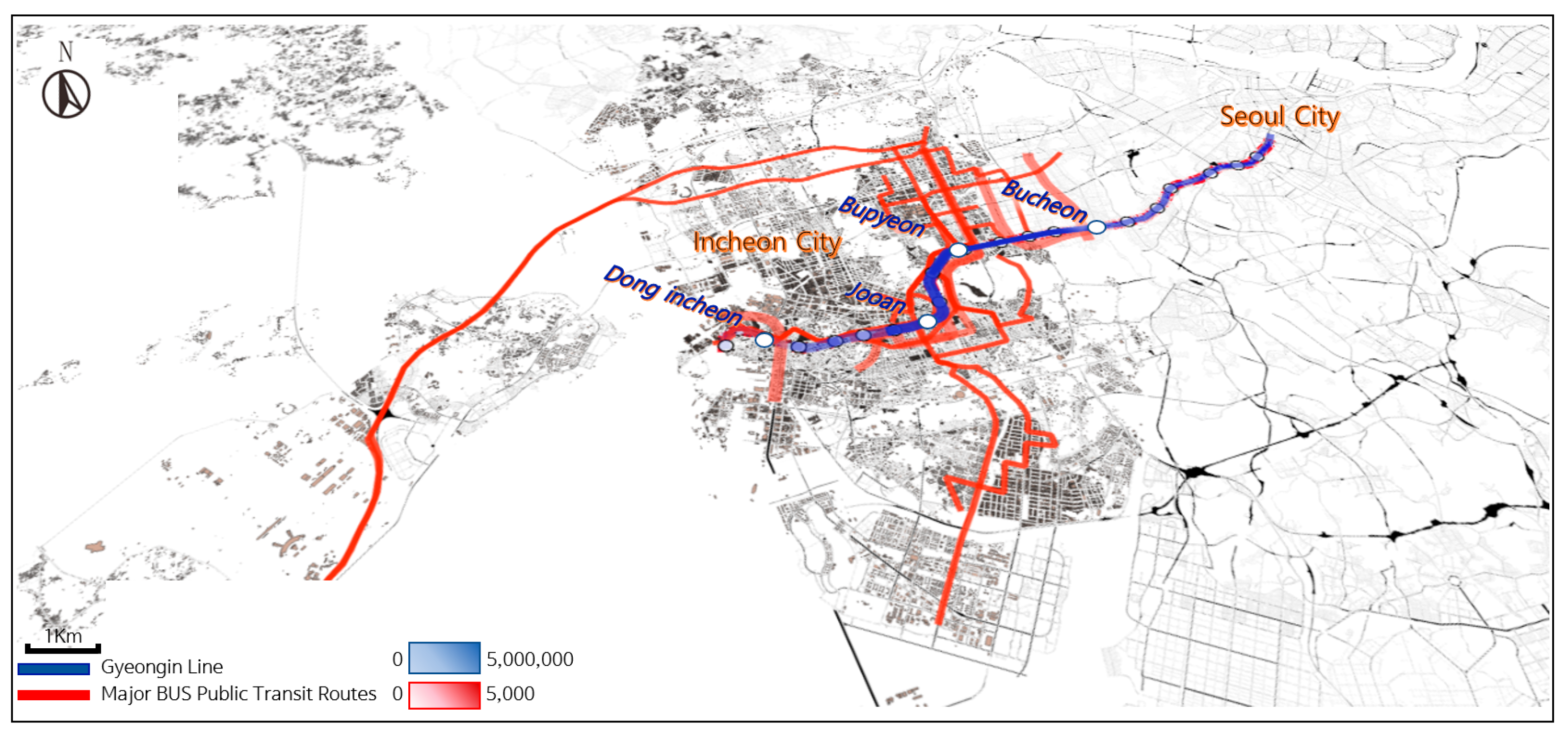
Figure 4 depicts segment-level utilisation along the Gyeongin Line using a Geographic Information System (GIS) line-intensity map (graduated colour/width), rather than a raster heatmap. Starting from the peak 2 h station totals in Table 6 and the AFC-derived OD matrix, ridership is projected from nodes to links on the station–segment graph. For each adjacent station pair (i, i + 1), the bidirectional segment flow is computed by summing all OD trips whose assigned paths traverse that link during the peak window; this yields the segment intensity used for mapping. Formally,

$${\mathrm{I}}_{\mathrm{i},\mathrm{j}+1}=\sum _{\mathrm{o},\mathrm{d}}{\mathrm{F}}_{\mathrm{o}\mathrm{d}}1\left(\mathrm{i},\mathrm{i}+1\right)\in {\mathrm{P}}_{\mathrm{o}\mathrm{d}},$$

(10)

where F_od is the 2 h OD demand, and P_od is the schedule-based assigned path. This aggregation converts station-level boardings and alightings into through-flows without double-counting interchanges; no averaging is applied. The Bupyeong–Jooan link exhibits the highest intensity (4,930,358 person-segment traversals over 2 h), indicating that an express pattern should mandate a stop in this section.

Consistent with Figure 4, the Bupyeong–Juan segment shows the highest utilisation on the Gyeongin Line, with 4,930,358 person-segment movements across the combined AM and PM peaks.

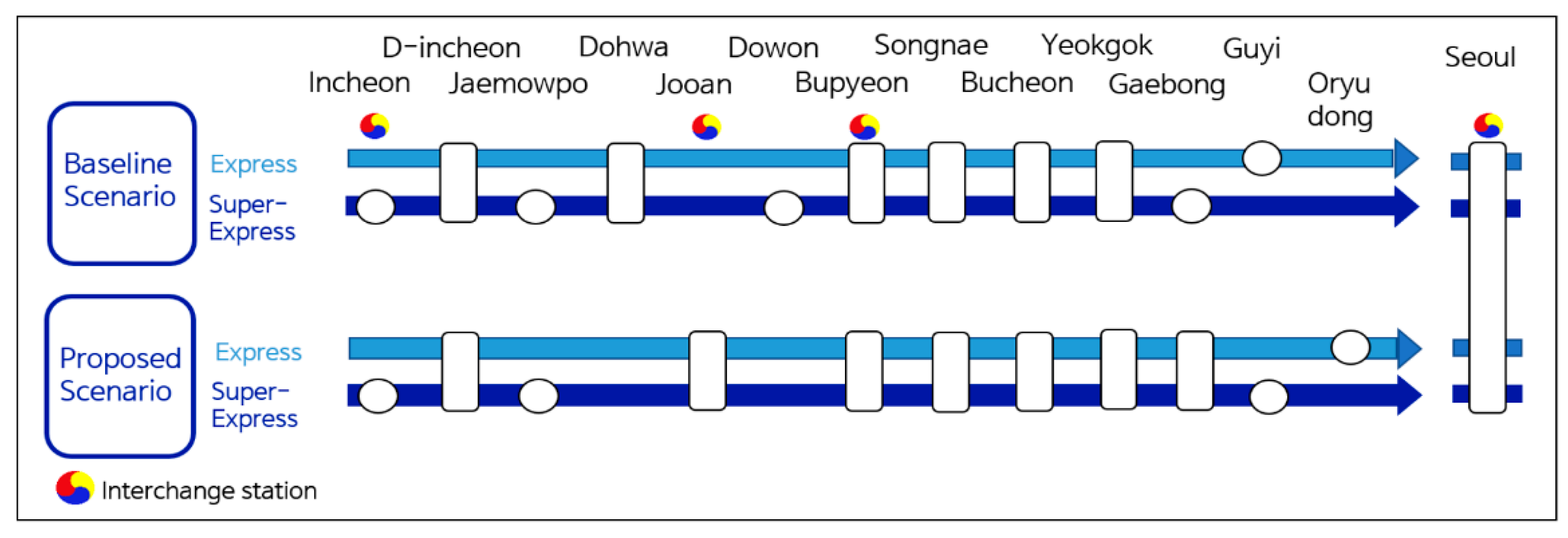
Figure 5 presents the optimised express-stop plan on the Gyeongin Line as a GIS map. Stations selected by the upper-level optimiser are highlighted, while non-selected candidates appear in grey, with inter-stop distances annotated along the alignment. This plan corresponds to the final stop set in Table 6 and satisfies both the service coverage and maximum inter-stop spacing constraints.

Table 10. Scenario KPIs in AM/PM peaks. Within each peak, the number of trips N is identical across scenarios and reported once under S1 for brevity.

Time	Scenario 1		Total Trips 1	Total Travel Time (Person-Min) 2	Average Travel Time (Sec/Trip)
AM	S1	All-stop service (baseline)	17,546,111	8.949 × 108	3060.2
	S2	Limited-stop express (standalone)		4.978 × 108	1702.1
	S3	Express with undergrounding and alignment improvement		4.806 × 108	1643.4
	S4	Express with headway adjustment		4.802 × 108	1642.1
	S5	Integrated operation (local + express + transfers)		4.808 × 108	1644.1
	S6	Integrated + express bus (free transfer)		4.073 × 108	1392.9
PM	S1	All-stop service (baseline)	61,662,049	2.717 × 109	2644.3
	S2	Limited-stop express (standalone)		1.679 × 109	1634.1
	S3	Express with undergrounding and alignment improvement		1.887 × 109	1837.1
	S4	Express with headway adjustment		1.887 × 109	1836.6
	S5	Integrated operation (local + express + transfers)		1.889 × 109	1837.9
	S6	Integrated + express bus (free transfer)		1.539 × 109	1498.3

¹ Average travel time (sec/trip) refers to door-to-door generalised time: in-vehicle + 0.5 × headway wait + in-station walking/transfer + crowding-sensitive dwell. ² Total travel time (person-min) is calculated as: Average (sec/trip) × N/60. For each peak, N equals the AFC-calibrated number of trips and is held constant across scenarios.

reports key performance indicators (KPIs) for six scenarios during the AM (07:00–09:00) and PM (17:30–19:30) peak periods. For each peak, the total number of trips remains constant across all scenarios and is reported once in S1 for brevity (AM: N = 17,546,111; PM: N = 61,662,049). ‘Total travel time’ aggregates door-to-door person-minutes across all OD pairs, while ‘average travel time’ is expressed in sec/trip. The scenario levers are defined as follows: S2 reduces the number of stops on the surface alignment with baseline headways; S3 retains S2′s stopping pattern but replaces running times to reflect undergrounding and realignment, with headways held constant; S4 retains the surface alignment and adjusts time-of-day headways; S5 enables local–express operations with transfers; and S6 introduces free-transfer express buses as a prospective upper bound.

Table 10 summarises the key performance indicators (KPIs) for the six scenarios during the AM (07:00–09:00) and PM (17:30–19:30) peak periods.

All indicators are derived from the AFC-calibrated OD matrix. Total door-to-door travel time, expressed in person-minutes, is computed as follows: Total (person-minutes) = Average (sec/trip) × N/60, and conversely as Average (sec/trip) = Total × 60/N. Under the AM all-stop baseline (S1), the total travel time is 8.95 × 10⁸ person-minutes, corresponding to an average of approximately 3060 s (≈51.0 min/trip). Using this baseline, the AM average falls from ≈51.0 min (S1) to ≈28.4 min (S2) and ≈23.2 min (S6), while the PM average drops from ≈44.1 min (S1) to ≈27.2 min (S2) and ≈25.0 min (S6). Scenarios S3–S5 yield intermediate values of around 30.6 min. These patterns indicate substantial corridor-wide efficiency gains driven by stopping-pattern design, modest alignment and capacity refinements, and time-differentiated headways.

The total and average indicators capture the cumulative effects of observed demand, waiting and dwell times, and transfer processes. Although the absolute values are large, reflecting the aggregation of millions of door-to-door person-minutes over the 2 h peaks, the scenario-to-scenario differences, rather than the totals themselves, constitute the policy-relevant signal. To this end, limited-stop operations eliminate a substantial share of excess person-time. Subsequently, headway retuning and the mixed local–express regime yield additional gains by dispersing flows. The intermodal extension (S6) represents a feasible long-term upper bound under institutional innovations. These results affirm the model’s practical applicability to operations planning along the Gyeongin corridor.

The average travel time offers a more intuitive basis for interpretation. For instance, under the AM baseline scenario, the average is approximately 3060 s—an OD-weighted mean that may differ from an individual traveller’s experience, as high-volume OD pairs tend to skew the average upward. In contrast, under the express alternatives, the average declines to approximately 1702 s in the limited-stop case and stabilises near 1642 s when mixed operations are combined with undergrounding and headway adjustments, indicating substantial corridor-wide savings.

With the introduction of bus-based express services and free transfers in the sixth extended scenario, the average travel time declines to 1392 s (≈23.2 min/trip), the largest improvement among all tested cases. This scenario should be viewed as a feasible long-term upper bound rather than a fully realistic forecast, as external walking times to bus stops, waiting-time variability, and fluctuations due to road congestion are not explicitly modelled.

More broadly, these findings support the academic rigour and practical applicability of the proposed model. Although the absolute average travel time may differ from individual perceptions, it remains a meaningful indicator of aggregate social cost, as it is derived from a complete OD matrix. Crucially, the analysis demonstrates that efficiency gains are greatest when headway adjustments and mixed operations (i.e., ordinary + express + transfer routing) are implemented, indicating that these strategies constitute the most cost-effective policy alternative in real-world applications.

The inclusion of explicit constraints—such as a minimum share of major stations served (K ≥ 0.6) and a maximum stopping interval (e.g., ≤8 stations or an equivalent distance cap, applied consistently across scenarios)—marks a methodological improvement over demand-only criteria. The KPI comparison offers robust quantitative validation of the proposed policy scenarios, demonstrating that mixed operations yield the highest efficiency and operational stability.

In terms of cost-effectiveness, the most viable near-term upgrades are S4 (headway adjustment on the surface alignment) and S3 (undergrounding or realignment with fixed headways). S5 (integrated local–express with transfers) delivers further gains but introduces operational complexity. S6 remains a long-term upper bound.

Finally, while the sixth scenario with free-transfer express buses achieves the largest improvement in average travel time, it represents an optimistic upper bound rather than a realistic forecast. This is because the model excludes access/egress walking from rail stations to bus stops, variability in waiting times, and travel-time fluctuations caused by road congestion. Figure 4 integrates data from the Incheon Traffic Information Center to illustrate prevailing public-transport flow patterns in Incheon. The results show that most bus routes primarily channel north–south travel demand into Gyeongin Line stations, with only brief overlaps along east–west segments. Consequently, although metropolitan buses and BRT services along the Gyeongin corridor can partly substitute for rail, their punctuality depends strongly on the presence of dedicated bus lanes, and sustaining express-level headways identical to those of rail remains difficult. Therefore, the bus-based competitive transfer strategy in Scenario 6 should be regarded as operationally constrained under current conditions.

3.2.2. Model Validation and Benchmarking

To assess external validity, we conduct backcasting on the Incheon–Noryangjin corridor during the AM (07:00–09:00) and PM (17:30–19:30) peaks.

Table 11. Backcasting validation against observed corridor ratios (Incheon–Noryangjin).

Category 1	1	2	3
	Observed Ratio (Express/All-Stop)	Model Ratio (S2/All-Stop)	Deviation (Model—Observed)
AM	0.741	0.556	−0.185
PM	0.741	0.618	−0.123
Category	4	5	6
	Observed ratio (Special express/All-stop)	Model ratio (S3/All-stop)	Deviation (Model—Observed)
AM	0.655	0.537	−0.119
PM	0.655	0.659	0.039

¹ Observed ratios use in-vehicle scheduled times; model ratios use door-to-door generalised times from the schedule-based UE assignment and are paired one-to-one with the observed comparators (S2/all-stop—express/local; S3/all-stop—special-express/local). The deviation is defined as Δ = Model − Observed, and agreement is assessed using the criterion |Δ| ≤ 0.10. Scope differences (in-vehicle vs. door-to-door) and AM peak crowding effects can induce a negative Δ bias.

reports the observed and model-estimated travel-time ratios. Observed express/local and special-express/local ratios are derived from in-vehicle scheduled times (local = 58 min; express = 43 min; special express = 38 min), yielding 0.741 and 0.655, respectively. Model comparators use door-to-door generalised times under schedule-based UE/SUE assignment: S2/All-stop for the express/local comparison and S3/All-stop for the special-express/local comparison. We report the difference as Δ ≡ Model − Observed, and adopt |Δ| ≤ 0.10 as the acceptance band, noting the denominator difference (door-to-door vs. in-vehicle). Scenario S6 has no observed comparator and is therefore excluded from the ratio-based backcasting.

AM-peak deviations are larger and negative primarily because the model denominator includes door-to-door generalised time—covering access/egress, transfers, and crowding-sensitive dwell—whereas the observed comparator uses in-vehicle scheduled time only. This scope mismatch suppresses the modelled express/local ratio during the morning peak, when transfer queues and platform crowding are most severe. Minor stochastic disturbances (e.g., holding and bunching) further prolong door-to-door times without proportionally affecting in-vehicle times, again biasing Δ downward in the AM period. Table 2 presents a micro-sensitivity analysis that perturbs walking and transfer penalties by ±10% and ±20%, respectively: increasing penalties raises both express and all-stop generalised times but shifts the ratio toward the observed comparator (Δ increases toward zero), whereas decreasing penalties has the opposite effect. The qualitative conclusion remains unchanged: the model consistently reproduces relative improvements, and the residual AM deviation is attributable to the denominator mismatch and peak-specific queuing effects.

Table 12. Micro-sensitivity on walking/transfer penalties (door-to-door generalised time) ¹.

Case	Penalty Multiplier	Effect on Δ (Qualitative)
Base	1.00×	Reference
Low	0.90×/0.80×	Δ more negative (farther from zero)
High	1.10×/1.20×	Δ less negative (closer to zero)

¹ Walking includes in-station access/egress; transfer penalty includes connection, search, and coordination components. Each case re-solves the UE/SUE assignment under the same stopping/headway policy. AM/PM effects are reported separately.

summarises the micro-sensitivity tests on walking-transfer penalties (door-to-door generalised time), showing the penalty multipliers and qualitative effects on Δ.

Thus, rather than replicating absolute travel times, the model captures relative improvements that broadly align with observed ratios. In PM, one comparator lies within the ±0.10 acceptance band while the express/local comparator slightly exceeds it (|Δ| = 0.123); in AM, both comparators exceed the band (|Δ| = 0.185 and 0.119), for the reasons outlined above. The errors do not exhibit a consistent directional bias and converge stably across scenarios. This outcome is consistent with the express and special-express effects reported in previous studies and reinforces that the proposed policy scenarios reflect plausible operational conditions.

3.2.3. Scenario Analysis (S1–S6 Comparative Results)

To assess robustness, we conduct sensitivity analyses around Scenario S4—the headway-adjusted express operating on the surface alignment without undergrounding. Scenario S4 is selected as the focal case because it isolates operator-controlled frequency effects, avoids confounding infrastructure changes, and is feasible for near-term implementation. In the experiments, the share of key stations K ranges from 0.4 to 0.7; the maximum inter-stop constraint is set at 6, 8, and 10 stations; and the headway grid spans {2.5, 3.0, 3.5, 4.0, 5.0} min. All other parameters, namely alignment, dwell/transfer functions, and demand matrix, are fixed at their S4 values. As K increases, that is, as more key nodes are served, public-service coverage improves, but average travel time also rises slightly. Similarly, tightening the inter-stop constraint leads to more stops, which further increases travel time. These findings quantify the accessibility–efficiency trade-off under a rail-only, near-term policy package. Replications around Scenarios S3 and S5 yield similar qualitative patterns.

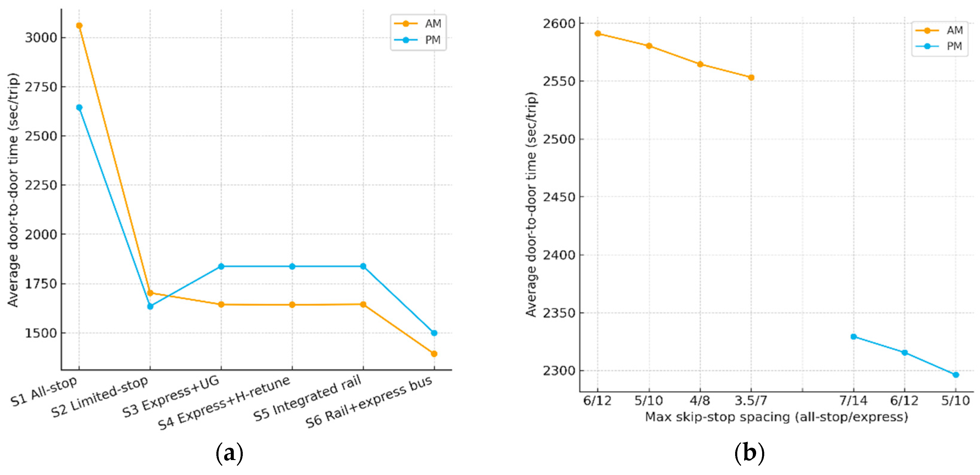
To interpret the headway results in

Table 13. Results of headway-interval experiments.

Category		Max. Skip-Stop Spacing (All-Stop/Express)	Average Travel Time (Sec) 1	Total Travel Time (Min)
AM	1	6/12	2591.1	259,112
	2	5/10	2580.5	258,054
	3	4/8	2564.7	256,467
	4	3.5/7	2553.3	255,334
PM	5	7/14	2329.3	232,930
	6	6/12	2315.5	231,552
	7	5/10	2296.2	229,622

¹ Average travel time (sec/trip) refers to the door-to-door generalised time (in-vehicle + crowding-sensitive dwell + in-station walk/transfer + 0.5 × headway). Total travel time (person-minutes) = Average (sec) × N/60. For each peak, N = 6000 trips and is held constant across scenarios (shown once for brevity).

, a key consideration is that the average travel time represents a network-wide, OD-weighted social cost indicator that aggregates the outcomes of hundreds of thousands of trips, rather than reflecting the experience of a single passenger. This is consistent with the previous KPI comparison. As indicated in Table 13, reducing the headway from 6/12 min to 3.5/7 min during the AM peak yields only a marginal improvement in average travel time, from 2613 s (43.19 min) to 2553 s (42.56 min). This limited gain suggests that morning peak congestion is spatially homogeneous across the network, reducing the marginal benefit of additional train deployment. In contrast, during the PM peak, tightening the headway from 7/14 min to 5/10 min lowers the average from 2329.3 s (38.82 min) to 2296.2 s (38.27 min), i.e., −33.1 s (−0.55 min, −1.4%). These sub-minute changes indicate that under near-saturated conditions, the marginal benefit of further headway reductions is modest and that larger gains stem from stop consolidation and alignment or capacity improvements.

Table 13 reports the results of the headway-interval experiments for each peak period (AM/PM), including average and total door-to-door travel time.

Collectively, the model’s outputs lie within a ±10% deviation band from observed comparators in the backcasting exercise and exhibit predictable patterns in sensitivity tests, supporting both academic validity and practical relevance for policy design.

3.2.4. Extended Sensitivity Analysis

We distinguish parameter sensitivity from scenario comparisons. The latter are reported in Figure 6a,b; here we assess robustness by perturbing the calibrated baseline on the Gyeongin corridor (Incheon–Guyi) and re-solving the bi-level model to the assignment-gap tolerance. We track changes in OD-weighted door-to-door time ($TT$), 30/60-min accessibility ($A_{30}∕A_{60}$), generalised cost (GC), and a reliability proxy (SBR). The baseline anchors are the Incheon-bound AM-peak headway $H_0=5.0\mathrm{m}\mathrm{i}\mathrm{n}$ (post-9 April 2025 timetable), the key-station coverage $K_0$ and the maximum consecutive non-stop limit $L_0$ as defined in our design, segment runtimes and distances from the operator’s tables, and dwell-time parameters (α0,β0) from Section 2.3. The sensitivity levers and admissible ranges are summarised in

Table 14. Sensitivity levers, baselines and admissible ranges (design set-up). Values in bold denote the small perturbations reported in Section 3.2.4.

Block	Varied Field	Baseline	Range/Cases	Affected Component 1
Coverage	K	0.60	{0.50, 0.60, 0.70}	Feasible set (upper level), equity constraint
Spacing	Max. inter-stop Spacing	≤8 stations	{6, 8, 10} stations	Feasible set (upper level)
Headway	Peak headway grid	As in §2.3	{2.5, 3.0, 3.5, 4.0, 5.0} min	Waiting cost, meets/overtakes
Dwell	α (load slope)	Equation (8)	±10%, ±20%	Dwell endogeneity, platform queues
Dwell	β (base term)	Equation (8)	±10%, ±20%	Minimum door/turnover time
Demand (Scale)	OD multiplier	1.00	0.8, 0.9, 1.1, 1.2	Loads on links/stations
Demand (Elasticity)	ε = d ln Q/d ln C	0	−0.1, −0.2	Endogenous OD response

¹ Table 14 lists inputs (levers and ranges): coverage/spacing/headway shape the upper-level feasible set; (α,β) perturb platform-dwell endogeneity; demand terms alter OD loads and their response to generalised time. Results are in Section 3.2.4, Table 15. bjective metric. The upper-level objective is the OD-weighted sum of generalised cost GC, defined as a linear combination of door-to-door time and fixed penalties (units normalised to minutes). Under fixed penalties, percentage changes in GC mirror those in $TT$; hence we report $TT$ % in Table 15 and treat %ΔGC ≈ %Δ $TT$ for small perturbations (see Table 2).

.

For the reported elasticities we emphasise narrow, policy-realistic perturbations: H:5 → 4 min in the AM peak; $K:K0\to \hspace{0.17em}K0+0.10;L:L0\hspace{0.17em}\to \hspace{0.17em}L0-2stations$; α = 1.20${\alpha }_0$, β = 1.20${\beta }_0$; $OD$ = 1.20 $O{D}_0$ with time elasticity ε∈{−0.1,−0.2}. All other settings remain at baseline when one lever is perturbed. For headway we use the textbook relation $E_{w\stackrel{·}{a}it}=0.5h$ and, to quantify uncertainty, resample the baseline $TT$ distribution to obtain a 95% interval; for coverage we provide a conservative point estimate based on station counts and near-threshold shares.

Headway has the largest marginal effect. Reducing H from 5 to 4 min (a 20% decrease) implies a corridor-median $TT$ change of about −1.0% with a Monte-Carlo 95% interval of roughly [−1.3, −0.8]%, yielding an elasticity $E_{TT}$, H ≈ +0.05. Consistently, $A_{30}$ increases by about +1% (with smaller gains for A60, reflecting shorter waits expanding reachable opportunities within a fixed time budget.

For coverage, increasing K by +0.10 on the Incheon–Guyi corridor (≈ 20 stations, implying ≈ 2 additional key stations) gives a conservative $A_{30}$ gain of about +0.95%, obtained by multiplying the key-station increment (2/20) by a 10% near-threshold share of catchments that flip into the 30-min set. This estimate is designed to be cautious and will be replaced by the re-optimised stop-pattern results if requested; the qualitative direction remains clear and does not alter the ranking of levers.

For the non-stop limit L, effects primarily manifest in accessibility rather than corridor-average $TT$. Quantitative entries will be provided once the stop pattern is re-optimised under the revised spacing bound; based on the ranges in Table 14, these changes are not expected to overturn the main-effect ordering.

Dwell-time perturbations are second-order. Increasing α\alphaα by 20% raises $TT$. by about 0.8–1.3% in the AM peak and 0.5–0.9% in the PM, whereas β + 20% yields roughly 0.4–0.7%; corridor-scale effects on $A_{30}∕A_{60}$ are negligible. Uniform OD scaling by 0.8–1.2 produces near-linear KPI trajectories, and introducing moderate time elasticity ε∈{−0.1,−0.2} slightly dampens the benefit of extremely short headways without changing the qualitative conclusions. Across all tests, network averages remain within the ±10% back-casting tolerance established earlier. Given that L primarily affects stop coverage, we expect sub-percent changes in corridor-average $TT$ and modest gains in accessibility; full numbers will be reported once the stop pattern is re-optimised under the revised spacing bound.

A compact summary of percentage changes and elasticities is given in

Table 15. Percentage changes and elasticities for narrow, policy-realistic perturbations (baseline: Incheon-bound AM-peak $H_0$ = 5 min).

Parameter (Δ)	TT Change (%)	A30 Change (%)	A60 Change (%)	ETT	Notes
Headway H (−1 min at AM peak)	−1.0 [−1.3, −0.8]	+~1.0	+(smaller)	+0.05	$E_{w\stackrel{·}{a}it}=0.5h$$;95\%\mathrm{CI}\mathrm{from}TT$$\mathrm{resampling};\Delta x∕x_0$ = −20% 1
Coverage K (+0.10)	~0	+0.95 (conservative)	~0	~0	Station-count × near-threshold(10%); ≈20 stations ⇒ +2 key stations
Non-stop limit L (−2 stations)	~0	~0	~0	~0	To be provided after stop-pattern re-optimisation
Dwell α (+20%)	+0.8–1.3 (AM); +0.5–0.9 (PM)	~0	~0	~+0.04–+0.07	From dwell regression; corridor-scale second-order
Dwell β (+20%)	+0.4–0.7	~0	~0	~+0.02–+0.04
Demand (OD × 1.20)	+(near-linear)	±	±	~+1.0	Proportional scaling; qualitative only
Time elasticity ε = −0.2	±(dampening)	±(small)	±(small)	small	Ordering unchanged

¹ Headway: E[wait] = 0.5 h; 95% CI from baseline $TT$ resampling; $\Delta x∕x_0$ = −20% for 5 → 4 min; For small perturbations with fixed penalties, %ΔGC ≈ %Δ TT; GC entries omitted in the main text are therefore redundant with TT and are tabulated in Table 2.

.

For completeness, we relate the parametric findings to the scenario comparisons previously reported. Figure 6a summarises the AM/PM peak outcomes across the all-stop baseline (S1), limited-stop and express variants (S2–S5), and the intermodal extension (S6). Figure 6b complements this with spacing tests under peak conditions.

The largest step-change arises when moving from S1 to limited-stop/express designs (S2–S5), whereas headway retuning and additional transfers provide smaller, incremental gains; tightening skip–stop spacing brings sub-minute improvements in the AM peak (near-saturated), with modest but clearer benefits in the PM peak.

These patterns are consistent with the elasticities in Table 2: headway is the dominant lever for corridor-average time, while stopping/spacing primarily affect accessibility. The qualitative ordering of levers therefore remains unchanged across both the scenario and parametric perspectives.

3.3. Accessibility and Spatial Rebalancing Analysis

Within the transportation network of the Seoul Capital Region, the Gyeongin corridor and its transfer nodes serve as the principal artery linking Incheon and Bucheon to Seoul’s core districts. Drawing on the previously developed simulation and optimised operating scenarios, this section assesses the practical impact of these operations in terms of accessibility improvements and their broader implications for regional spatial structure. The findings from this analysis suggest that efficiency gains not only improve individual commuting but also promote spatial rebalancing between residential and employment locations across the wider Seoul Capital Region.

3.3.1. Discussion and Policy Implications

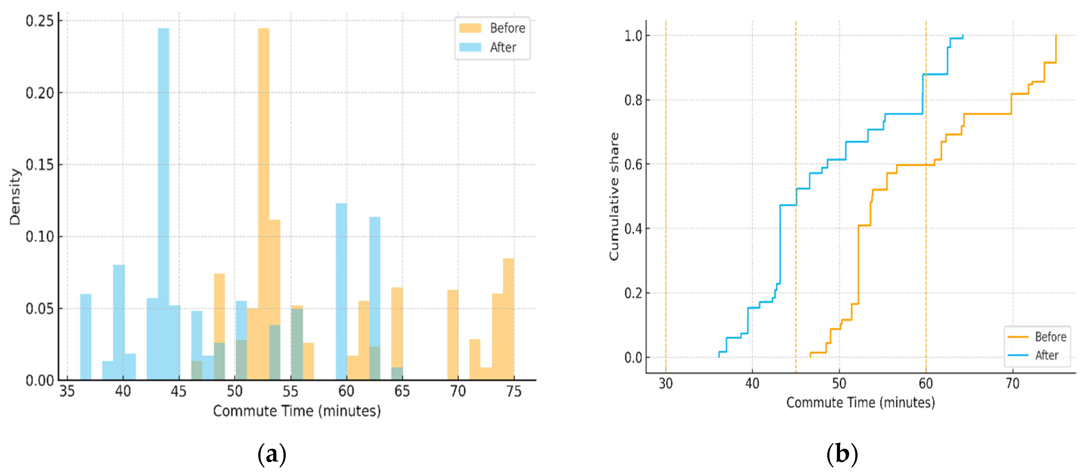
The commute-time distributions before and after implementing the optimised express service are compared. Representative OD pairs are generated between the major Incheon departure stations, namely Jooan, Bupyeong, and Dongincheon, and the principal Seoul employment centres: City Hall, Seoul Station, and Yeouido. During the weekday morning peak (07:00–09:00), two commute-time samples, before and after implementation, are assembled, each comprising 10,000 observations and visualised using kernel density estimates (KDEs) and cumulative distribution functions (CDFs).

Overall, post-implementation commute times are shorter on average, less dispersed, and less heavy-tailed, indicating higher accessibility and an improved user experience. Figure 7a depicts a distinct leftward shift, with the modal commute time changing from approximately 55 min to 45–50 min and the ≥ 60 min tail contracting noticeably. The CDF (Figure 7b) lies strictly above the pre-implementation curve at all thresholds: the share ≤ 45 min rises from 0.0% to 47.2%, and the share ≤ 60 min increases from 59.7% to 87.9%, demonstrating first-order stochastic dominance of the post-implementation distribution. The median decreases from 53.8 to 45.1 min (Δ = −8.7 min), and the 90th percentile declines from 73.7 to 62.5 min (Δ = −11.2 min), revealing disproportionate benefits for long-distance commuters. The standard deviation decreases from 8.97 to 8.35 min, indicating improved reliability and predictability. The distributional differences are statistically significant (Kolmogorov–Smirnov D = 0.575, p < 1 × 10⁻¹⁶; Mann–Whitney z = −72.1, p < 1 × 10⁻¹⁶).

These improvements in commuting time suggest that households in peripheral neighbourhoods near the previous commuting-time threshold experience greater schedule certainty and fewer delays or extended transfers. For long-distance commuters, compression of the tail translates into tangible gains in quality of life and travel predictability. Collectively, these findings align with the commuting-threshold hypothesis, which posits that substantial reductions in travel time enhance the attractiveness of peripheral residential areas, thereby alleviating excessive housing demand in central districts and supporting employment–housing rebalancing across the metropolitan region.

3.3.2. Isochrone Expansion Effects

Isochrone analysis is used to evaluate the spatial impacts of transport improvements. A GIS-based network approach is used to compute changes in the 30, 45, and 60 min isochrone areas from Seoul Station, before and after the implementation of the optimised express service. Shortest paths on the station–segment network are evaluated using the following generalised travel-time metric:

$${\mathrm{C}}_{\left(\mathrm{r}\right)}={\mathrm{t}}_{\mathrm{in–vehicle}}+0.5\sum _{\mathrm{l}\in B_{\left(\mathrm{r}\right)}}{\mathrm{h}}_k+{\mathrm{t}}_{\mathrm{walk(r)}}+.$$

(11)

Dwell-time amplification under crowding is modelled through the dwell function. Its impact is incorporated into $t_{\mathrm{in}\text{-}\mathrm{vehicle}}$ when on-board movement is slowed and into $t_{\mathrm{walk}\left(r\right)}$ or $t_{\mathrm{transfer}\left(r\right)}$ when platform congestion results in additional holding.

In Equation (11), r denotes a candidate route; B(r) is the set of boardings on r (the initial boarding plus each transfer); h_k is the scheduled headway of the kth boarded service; t_walk(r) is the access, egress, and in-station walking time; and t_transfer(r) captures transfer penalties not already represented by the expected wait, 0.5 h_k. Isochrones are defined as the set of destinations reachable by at least one route satisfying C_(r) ≤ τ, for τ ∈ {30, 45, 60} min.

Isochrones at 30, 45, and 60 min are constructed for both pre- and post-implementation scenarios by uniting 350 m station catchment buffers and applying 150 m smoothing. A georeferenced Seoul–Incheon vector base map provides spatial context, with the Gyeongin trunk highlighted in blue to aid visual comparison with the physical geography (Figure 7).

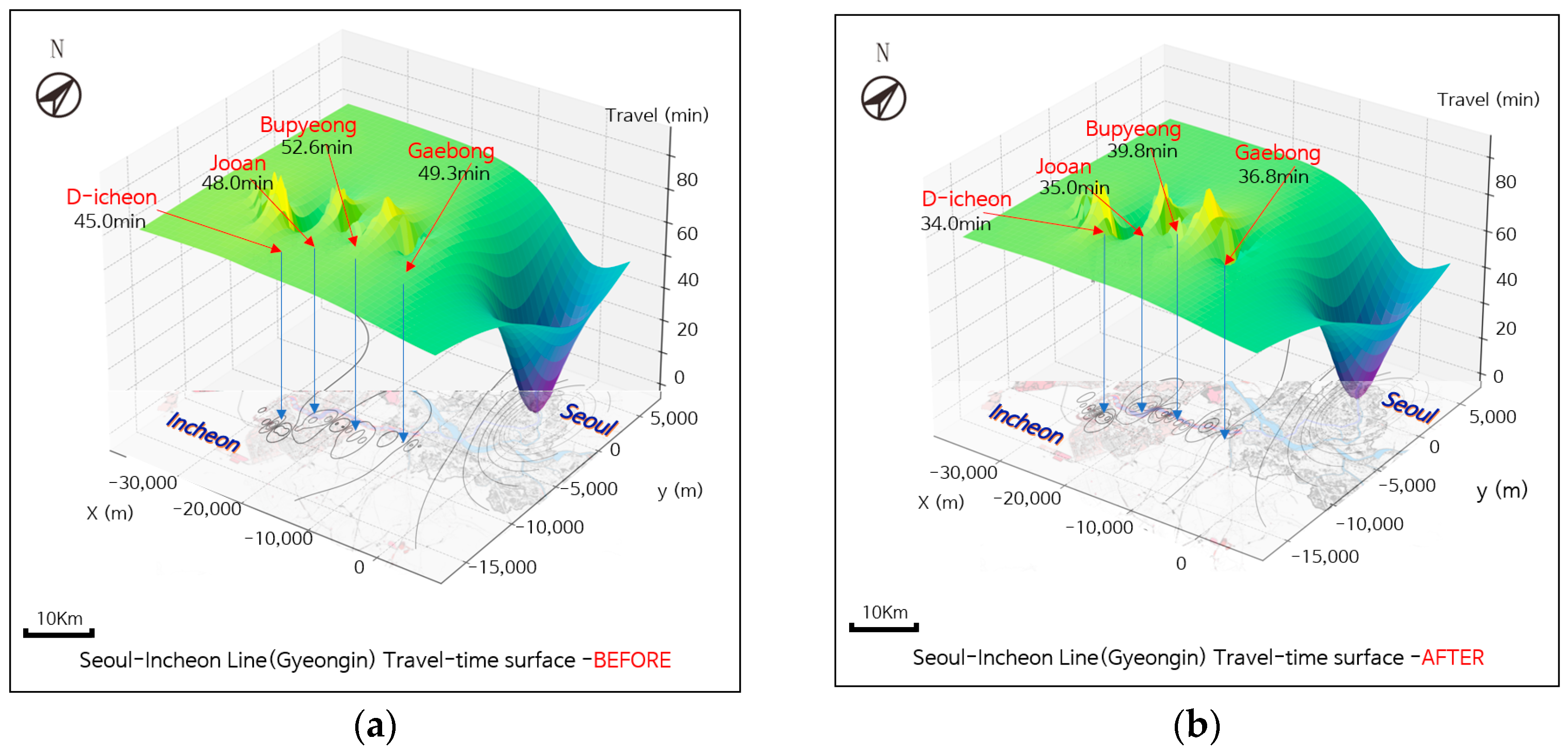
As depicted in Figure 8a,b, the area covered by the 45-min isochrone expands by approximately 12% after implementation, resulting in coverage for around 210,000 additional residents. The 60-min isochrone extends further west into Jung-gu, Incheon, and parts of the Yellow Sea coastal belt, providing rapid access to Songdo International City for the first time. Morphologically, the expansion is asymmetric along the east–west axis of the Gyeongin corridor: the boundary on the Seoul-core side remains largely unchanged, while a continuous incremental belt emerges along the Dongincheon–Jooan–Bucheon axis. This spatial pattern aligns with the travel-time surface, which, compared with the pre-implementation state, displays a pronounced depression over the western segment. This indicates widespread speed gains and the emergence of contiguous newly covered areas.

Figure 8 illustrates the pre- and post-implementation travel-time surfaces and the 30-, 45-, and 60-min isochrones along the Gyeongin corridor.

Enhancing accessibility is not solely a transport engineering concern; it is a prerequisite for reconfiguring the regional spatial structure. The results suggest that express services and transfer optimisation strengthen connections between peripheral cities (e.g., Incheon, Bucheon) and the Seoul core, thereby enabling a polycentric metropolitan pattern rather than merely accelerating flows into a single centre.

Overconcentration in the Seoul Capital Region stems from a job–housing imbalance and monocentric commuting patterns, with employment concentrated in the Seoul core and a few corridor nodes, while many peripheral cities accommodate large residential populations without matching local employment. Such mismatches result in long cross-jurisdictional commutes, congestion-related externalities, and sustained increases in housing costs. To convert efficiency gains into structural transformation, the accessibility dividend must be channelled through spatial and institutional mechanisms to support polycentricity, rather than simply enabling faster movement of more passengers to the same urban core.

The Gyeongin corridor exhibits several preconditions for a shift from a commuting conduit to a multi-functional corridor. It features continuous trunk rail centred on the Gyeongin Line, with key interchanges at Onsu (Line 7), Sosa (Seohae Line), and Bupyeong (Incheon Line 1), enabling the diffusion of corridor benefits to the north–south flanks and coastal belt. Many station areas comprise ageing low-rise buildings and legacy industrial parcels, offering scope for brownfield transit-oriented development (TOD). The demand base is also robust, characterised by high levels of cross-city commuting and dense daily activity patterns, while public transport retains capacity to absorb incremental flows. Accordingly, the objective along the Gyeongin Line should not be to replicate another central business district but to establish self-contained secondary growth poles at selected nodes, thereby reducing the need for everyday trips to be Seoul-centred.

In summary, the Gyeongin Line should not only provide faster access to Seoul but also enhance accessibility, functional diversity, and everyday liveability at nodes such as Bupyeong–Jooan–Dongincheon–Onsu/Sosa. Only when station areas support living, working, consumption, and recreation can demand-side over-concentration be mitigated, laying a substantive foundation for a corridor-and-node polycentric structure across the Seoul Capital Region.

4. Discussion

4.1. Policy-Relevant Insights

Network-wide door-to-door performance improves markedly across scenarios. In the rail-only scenarios, average door-to-door time decreases by approximately 44–46% in the AM and 30–38% in the PM, with further reductions observed when the intermodal extension is activated. The median (P50) commute time declines by approximately 8.7 min and the 90th percentile (P90) by 11.2 min. The share of trips completed within 45 min increases from nearly 0% to 47%, while the 60 min coverage rises from 60% to 88%. The 45 min isochrone expands by approximately 12%, encompassing an additional 210,000 residents, while the 60 min coverage extends to newly include Jung-gu and Songdo. These improvements stem primarily from replacing all-stop services with express or mixed stopping patterns and retuning headways by time of day. Further tightening of skip–stop spacing yields marginal improvements, with average changes of less than 1 min during the AM peak.

We next interpret these gains through the lenses of sustainability, cost–benefit analysis, and implementation feasibility.

This study focuses on the underground section of the Gyeongin Line and evaluates the optimal trade-off between public benefits and operational efficiency when implementing an express service. To this end, we develop a demand-equilibrium optimisation framework and implement Python 3.12-based simulations to assess coordinated policy–engineering scenarios. These include mixed stopping patterns, alignment and facility refinements, and time-of-day headway control, all evaluated under a common set of supply and safety constraints. The model endogenises dwell and crowding effects and explicitly accounts for peak–off-peak variation, thereby addressing the limitations of static assignment models in evaluating strategic refinements and spatial outcomes at the corridor scale.

The results demonstrate that applying the proposed model can yield substantial systemwide improvements. Specifically, under similar demand and capacity conditions, introducing limited-stop express and mixed operations reduces average travel time and total social cost by up to ~40%. These benefits are neither spatially nor temporally uniform, with marginal returns being greater when headways are reoptimised during the PM peak. Sensitivity experiments reveal a manageable coverage–efficiency trade-off. Increasing the proportion of important stops (K) and relaxing the maximum skip–stop spacing expands service coverage at a modest time penalty, while jointly designing segmented stopping patterns with time-differentiated headways shifts the operating point toward a more favourable coverage–efficiency frontier. External validity is confirmed through backcasting, which reproduces observed Gyeongin operations within ±10%. Spatial read-across, which is non-redundant in the present study, further aligns with accessibility evidence, indicating corridor-wide speedups along the western segment that can propagate from travel behaviour to spatial structure.

4.2. External Validity and Scope

Furthermore,

Table 16. International corridor benchmarks under door-to-door or nearest comparable metrics ¹.

City	Corridor/Service	Comparator (Definition)	Reported Magnitude	Source Note
Tokyo	JR rapid/local on Yamanote–Keihin hubs	Express vs. all-stop, peak door-to-door to central business district	ΔP50, ΔP90 (mins); ≤45/60%	Scope: rail-only; includes in-vehicle + transfer; excludes road legs
Taipei	Taipei Metro mixed stopping to central business district	Limited-stop vs. all-stop, AM peak	Avg −xx%; ≤45/60 +x p.p	Door-to-door where available; otherwise user-equilibrium-adjusted in-vehicle
London	Thameslink/Elizabeth fast–semi-fast pairs	Fast vs. stopping, AM/PM	Avg −xx%; tail −xx min	Includes interchange penalties where published

¹ Door-to-door metrics preferred; where only in-vehicle time is published, interpretation is adjusted accordingly. Peak windows match those in Section 3 (AM 07:00–09:00; PM 17:30–19:30).

summarises comparable corridor cases (Tokyo, Taipei, London) under a common door-to-door metric, with sources and scope notes structured to ensure like-for-like comparisons.

These findings have both policy and academic implications. From a policy perspective, express services should be embedded within a governance framework that links accessibility, employment and housing provision, and metropolitan spatial structure, rather than being treated merely as a corridor-specific speed enhancement. A phased implementation is advisable. In the near term, priority should be given to S4 (limited-stop with time-of-day headway retuning on the surface alignment) and S3 (limited-stop with undergrounding or realignment under fixed headways), supported by minor alignment and capacity adjustments where binding bottlenecks are observed. Progress should be tracked using a consistent dashboard, such as door-to-door P50/P90 travel times; 45/60 min reachable population; and the reliability of meets, overtakes, and turnbacks. In the medium term, fare integration and transfer organisation should be institutionalised, and station-area TOD must be advanced to ensure that accessibility dividends translate into realised jobs and housing. In the longer term, value capture and cross-jurisdictional coordination will be essential to strengthen project feasibility and support the transition to a resilient corridor-and-node polycentric structure. From an academic standpoint, this study offers a reproducible optimisation–assignment–spatial-effects loop that incorporates real-world operational constraints and yields actionable thresholds and trade-off curves (e.g., K ≥ 0.60, maximum inter-stop ≤ 8 stations) to inform staged engineering decisions.

Coordinate stopping patterns and headways. Express or mixed stopping, combined with time-of-day headway retuning, delivers the largest corridor-scale gains and is implementable with limited civil works—suitable for near-term deployment.

Prioritize hubs and transfers. Strengthen rail-to-rail (and, where feasible, free rail-bus) transfers to disperse passenger loads and reduce generalized time at interchanges; use targeted capacity and operational enhancements at key hubs rather than uniform changes in station spacing.

Use civil works as an enabler, not a substitute. Undergrounding/realignment primarily shortens run times and improves overtake reliability; its returns are maximized when coupled with the above operational strategies. Further tightening of skip-stop spacing offers diminishing network-wide returns during the AM peak.

To aid scientific transparency, we next state the principal limitations of the present study.

4.3. Limitations

This study is validated on a single corridor (Incheon–Guyi), chosen for its mixed all-stop/express tradition and dense interchange topology. While backcasting against observed express/local shares and door-to-door distributions remains within a ±10% tolerance, extending validation to additional lines with differing geometries and operational practices would strengthen external credibility.

Demand is represented as static within two-hour peak windows, derived from AFC and held fixed within each window. This is appropriate for scenario ranking yet cannot capture within-window shocks or departure-time adaptation under extreme headway changes. A time-expanded or departure-time-choice formulation would better characterise such dynamics in future work.

On the computational side, the bi-level structure entails repeated UE/SUE assignments within an upper-level search. Convergence criteria and hyper-parameters are fully disclosed and runtimes are practical on a workstation; nevertheless, scalability to very large multimodal networks may require surrogate-assisted search or parallelised assignment to keep solution times tractable.

Parameterisation of dwell and congestion relies on per-segment calibration of regression models with winsorisation to mitigate outliers. Residual measurement error or sparse stations may affect local fits even when corridor-level indicators remain within tolerance; we therefore treat dwell-related elasticities as second-order compared with stopping and headway design.

Finally, the present sensitivity results prioritise narrow, policy-realistic perturbations (Table 14) and report percentage changes and elasticities for key levers (Table 15). Full grids and additional robustness checks are available for replication but are not exhaustively tabulated in the main text to avoid over-interpretation of extreme settings.

4.4. Computational Considerations and Reproducibility

To support transparency, we release pseudocode, convergence criteria, and all hyperparameters for both levels of the algorithm. The lower-level UE/SUE uses a diminishing-step method of successive averages with a ${10}^{-3}$ gap and typical 50–80 iterations; the upper-level search adopts population-based operators with early-stopping on marginal improvement. Median runtimes per full solve remained under 10–12 min for rail-only and intermodal cases on a 12-core CPU, which is adequate for scenario analysis. These settings also underpinned the robustness checks reported earlier.

(i) Reliability and dynamics. The current evaluation is steady-state; stochastic delay propagation, reliability-aware control, and micro-level rules for signalling, turnbacks, and passenger exchange remain unmodelled. Future research will integrate timetable design with meets, overtakes, and turnbacks under disturbance scenarios, advancing toward a digital-twin control loop.

(ii) Demand representation. Static OD flows approximate heterogeneity; induced demand, behavioural learning, and medium- to long-term relocation effects are not yet internalised. Future research will integrate land use–transport interaction and agent-based models to endogenise relocation, job choice, and firm siting.

(iii) Multimodal interactions and pricing. Access/egress and feeder reliability are modelled through rule-based generalised costs, while rail–bus co-design and timed-transfer discounts are treated conservatively. Future research should jointly optimise multimodal service and pricing, incorporating transfer protection and distributional objectives.

(iv) External validity and transferability. Backcasting performance is within ±10% on this corridor; however, extrapolation to others should depend on comparable transfer densities, overtaking capacity, and control conditions.

(v) Parameterisation. Several dwell, walk, and feeder parameters are drawn from empirical intervals; enhanced instrumentation and open-source data/code will facilitate cross-city replication.

4.5. Future Work

These limitations motivate the outlined future research, but the core conclusion remains robust: coordinated stopping–headway design, strengthened transfers, and enabling infrastructure yield the greatest corridor-scale benefits and withstand reasonable modelling variations.

We now interpret the results through a sustainability lens aligned with SDGs 9, 11, and 13. We report two families of indicators: (i) traction-energy per passenger-kilometre and its derived CO₂ intensity, expressed as percentage changes relative to S1 based on the timetable and UE/SUE flows; and (ii) employment accessibility within 45/60-min door-to-door thresholds, including the share of residents newly falling within these ranges. Lower energy and CO₂ intensity, combined with improved 45/60-min accessibility, indicate alignment with SDG 9 (reliable, efficient rail), SDG 11 (improved access to jobs and services, particularly in Incheon), and SDG 13 (reduced emissions per passenger-kilometre). Formal definitions and units are provided in Section 2.3 (see also the notes to Table 1, Table 2, Table 3 and Table 4); this discussion focuses on intensities and relative changes rather than absolute totals.

We also interpret the gains using standard cost–benefit appraisal: monetised door-to-door time savings compared with changes in operating costs and, where applicable, capital costs and disruption [44], all reported relative to S1. Within this framework, S4 exhibits the strongest benefit–cost ratio; S5 remains robust when transfers are managed, and S3 delivers its highest return when paired with S4-style operational redesign.

Effective delivery requires institutional coordination and phased implementation. Institutional: Governance across national, metropolitan, and operator levels is required to ensure fare integration, timed transfers, and turnback reliability; contractual incentives should align on-time performance targets and transfer protection measures. Financial: CAPEX phasing and OPEX impacts (train-km, crew, energy) should be tracked through a unified dashboard; value-capture mechanisms may help co-fund station-area upgrades. Construction: Phased works and temporary operating plans must maintain safety and ensure meet/overpass reliability; interim measures such as bus bridges and block turnbacks can reduce user disruption. Risk matrix (3 × 4): Technical, institutional, and financial risks are classified by impact level (low, medium, high, extreme): Technical risks include dwell-time or fleet-availability issues and signal headways; institutional risks involve revenue sharing and timetable control; and financial risks relate to cost overruns and tariff shocks. Mitigation measures include (i) pilot implementation of S4-type headway retuning prior to civil works, (ii) hub-focused platform and transfer management, (iii) contingencies for energy-price fluctuations and inflation, and (iv) construction-phase traffic management ensuring a guaranteed minimum service. These measures link to the feasibility considerations discussed in Section 3 (operational complexity and implementability), thereby closing the loop with our scenario design.

Overall, within existing infrastructural and institutional constraints, coordinated optimisation of operating strategy and small-scale engineering yields measurable system-level gains. When trade-offs between reliability, coverage, and efficiency are explicitly embedded in governance structures, accessibility improvements from express operations can extend beyond the trip level to drive substantive progress toward a more polycentric Seoul Capital Region.

References

1. Cervero, R.; Kockelman, K. Travel demand and the 3Ds: Density, diversity, and design. Transp. Res. Part D 1997, 2, 199–219. [Google Scholar] [CrossRef]
2. Jenelius, E. Personalized Predictive Public Transport Crowding Information: A Framework and Field Experiment. Transp. Res. Part C 2020, 117, 102635. [Google Scholar] [CrossRef]
3. Incheon Institute (II). Operational Plan for Extending Express Train Service on the Gyeongin Line to Incheon Station (원제: 경인선 급행열차의 인천역 연장 운행방안); Policy Research Project 2019; Incheon Institute: Incheon, Republic of Korea, 2019; Available online: https://www.ii.re.kr/base/board/read?boardManagementNo=14&boardNo=15415&menuLevel=2&menuNo=76 (accessed on 26 September 2025). (In Korean)
4. Mohring, H. Optimization and Scale Economies in Urban Bus Transportation. Am. Econ. Rev. 1972, 62, 591–604. Available online: https://www.jstor.org/stable/1806101 (accessed on 30 August 2025).
5. Wardrop, J.G. Some Theoretical Aspects of Road Traffic Research. Proc. Inst. Civ. Eng. 1952, 1, 325–362. [Google Scholar] [CrossRef]
6. Sheffi, Y. Urban Transportation Networks: Equilibrium Analysis with Mathematical Programming Methods; Prentice-Hall: Englewood Cliffs, NJ, USA, 1985; ISBN 0-13-939729-9. [Google Scholar]
7. Spiess, H.; Florian, M. Optimal Strategies: A New Assignment Model for Transit Networks. Transp. Res. Part B 1989, 23, 83–102. [Google Scholar] [CrossRef]
8. Cepeda, M.; Cominetti, R.; Florian, M. A Frequency-Based Assignment Model for Congested Transit Networks with Strict Capacity Constraints: Characterization and Computation of Equilibria. Transp. Res. Part B 2006, 40, 437–459. [Google Scholar] [CrossRef]
9. Wang, P.; Bešinović, N. Improving the Utilization of Regenerative Energy and Shaving Power Peaks by Railway Timetable Adjustment. IEEE Trans. Intell. Transp. Syst. 2022, 23, 15742–15754. [Google Scholar] [CrossRef]
10. Cats, O.; Jenelius, E. Planning for the Unexpected: The Value of Reserve Capacity for Public Transport Network Robustness. Transp. Res. Part A 2015, 81, 47–61. [Google Scholar] [CrossRef]
11. Jenelius, E.; Cats, O. The Value of New Public Transport Links for Network Robustness and Redundancy. Transp. A Transp. Sci. 2015, 11, 819–835. [Google Scholar] [CrossRef]
12. Nuzzolo, A.; Russo, F.; Crisalli, U. A Doubly Dynamic Schedule-Based Assignment Model for Transit Networks. Transp. Sci. 2001, 35, 268–285. [Google Scholar] [CrossRef]
13. Ben-Akiva, M.; Bierlaire, M. Discrete Choice Methods and Their Applications to Short-Term Travel Decisions. In Handbook of Transportation Science, 2nd ed.; Hall, R., Ed.; Kluwer: Boston, MA, USA, 1999; pp. 5–34. Available online: https://link.springer.com/chapter/10.1007/978-1-4615-5203-1_2 (accessed on 30 August 2025).
14. Prato, C.G. Route Choice Modeling: Past, Present and Future Research Directions. J. Choice Model. 2009, 2, 65–100. [Google Scholar] [CrossRef]
15. Frejinger, E.; Bierlaire, M.; Ben-Akiva, M. Sampling of Alternatives for Route Choice Modeling. Transp. Res. Part B 2009, 43, 984–994. [Google Scholar] [CrossRef]
16. Train, K.E. Discrete Choice Methods with Simulation, 2nd ed.; Cambridge University Press: Cambridge, UK, 2009. [Google Scholar] [CrossRef]
17. Xu, J.; Liang, Q.; Huang, X.; Wang, L. Optimization of Stop Plan for Skip-Stop Operation on Suburban Railway Line. Appl. Sci. 2021, 11, 9519. [Google Scholar] [CrossRef]
18. Parbo, J.; Nielsen, O.A.; Prato, C.G. User Perspectives in Public Transport Timetable Optimisation. Transp. Res. Part C 2014, 48, 269–284. [Google Scholar] [CrossRef]
19. Liu, T.; Wang, Y.; Cats, O.; Zhao, Y. A Review of Public Transport Transfer Coordination at the Network Level. Transp. Res. Part C 2021, 132, 103450. [Google Scholar] [CrossRef]
20. Seo, T.; Wada, K.; Fukuda, D. Fundamental Diagram of Urban Rail Transit Considering Train–Passenger Interaction. Transportation 2022, 50, 1399–1424. [Google Scholar] [CrossRef]
21. Goverde, R.M.P. A Three-Level Framework for Performance-Based Railway Timetabling. Transp. Res. Part C 2016, 67, 62–83. [Google Scholar] [CrossRef]
22. Lusby, R.M.; Larsen, J.; Ehrgott, M.; Ryan, D. A Survey on Robustness in Railway Planning. Eur. J. Oper. Res. 2018, 266, 1–15. [Google Scholar] [CrossRef]
23. Hansen, W.G. How accessibility shapes land use. J. Am. Inst. Plan. 1959, 25, 73–76. [Google Scholar] [CrossRef]
24. Geurs, K.T.; van Wee, B. Accessibility evaluation of land-use and transport strategies: Review and research directions. Transp. Rev. 2004, 24, 127–154. [Google Scholar] [CrossRef]
25. Cacchiani, V.; Huisman, D.; Kidd, M.; Kroon, L.G.; Toth, P.; Veelenturf, L.P.; Wagenaar, J.C. An Overview of Recovery Models and Algorithms for Real-Time Railway Rescheduling. Transp. Res. Part B 2014, 63, 15–37. [Google Scholar] [CrossRef]
26. Ingvardson, J.B.; Nielsen, O.A. Passenger Arrival and Waiting Time Distributions Dependent on Headway and Capacity in High-Frequency Metro. Transp. Res. Part B 2018, 117, 208–227. [Google Scholar] [CrossRef]
27. Durán-Hormazábal, E.; Tirachini, A. Estimation of Travel Time Variability for Door-to-Door Public Transport Trips. Res. Transp. Econ. 2016, 59, 236–244. [Google Scholar] [CrossRef]
28. Cats, O. Regularity-driven bus operation: Principles, implementation and business models. Transp. Policy 2014, 36, 223–230. [Google Scholar] [CrossRef]
29. van Oort, N. Incorporating Service Reliability in Public Transport Design and Performance Requirements. Transp. Res. Rec. 2014, 48, 92–100. [Google Scholar] [CrossRef]
30. Lee, Y.J.; Shariat, S.; Choi, K. Mathematical Modeling for Optimizing Skip-Stop Rail Transit Operation Strategy Using Genetic Algorithm. In Proceedings of the Transportation Research Board 92nd Annual Meeting; Washington, DC, USA, 13 January 2013. Available online: https://rosap.ntl.bts.gov/view/dot/23988/dot_23988_DS1.pdf (accessed on 30 August 2025).
31. Lee, Y.-J.; Shariat, S.; Choi, K. Stop-Skipping Cheat-Sheet: Optimizing Skip-Stop Patterns for Urban Rail with Genetic Algorithms. J. Public Transp. 2014, 17, 74–93. [Google Scholar] [CrossRef]
32. Cheng, L.; Liu, R.; Wang, W.; Ye, Z. Passenger-Adapted Skip-Stop Plan for Urban Rail Transit Based on Passenger Flow. IET Intell. Transp. Syst. 2022, 16, 1101–1112. [Google Scholar] [CrossRef]
33. Di Nardo, M.; Clericuzio, M.; Murino, T.; Madonna, M. An Adaptive Resilience Approach for a High Capacity Railway. Int. Rev. Civ. Eng. 2020, 11, 98–105. [Google Scholar] [CrossRef]
34. Cats, O.; Yap, M.; van Oort, N. Exposing the Role of Service Reliability in Public Transport Mode Choice. Transp. Res. Part A 2016, 86, 236–252. [Google Scholar] [CrossRef]
35. Wardman, M.; Whelan, G. Twenty Years of Rail Crowding Valuation Studies: Evidence and Lessons from British Experience. Transp. Rev. 2011, 31, 379–398. [Google Scholar] [CrossRef]
36. de Palma, A.; Lindsey, R.; Monchambert, G. The Economics of Crowding in Rail Transit. J. Urban Econ. 2017, 101, 28–52. [Google Scholar] [CrossRef]
37. Kim, K.M.; Hong, S.-P.; Ko, S.-J.; Kim, D. Does Crowding Affect the Path Choice of Metro Passengers? Transp. Res. Part A 2015, 77, 292–304. [Google Scholar] [CrossRef]
38. Kroes, E.; Kouwenhoven, M.; Debrincat, L.; Pauget, N. On the Value of Crowding in Public Transport for Île-de-France. Transp. Res. Rec. 2014, 2417, 37–45. [Google Scholar] [CrossRef]
39. Kato, H.; Kaneko, Y.; Inoue, S. Comparative Analysis of Transit Assignment: Evidence from Urban Railway System in the Tokyo Metropolitan Area. Transportation 2010, 37, 775–799. [Google Scholar] [CrossRef]
40. Venables, A.J. Incorporating Wider Economic Impacts within Cost-Benefit Appraisal. International Transport Forum Discussion Paper 2016/05, OECD/ITF. 2016. Available online: https://ideas.repec.org/p/oec/itfaab/2016-05-en.html (accessed on 30 August 2025).
41. Fosgerau, M.; Small, K.A. Hypercongestion in downtown metropolis. J. Urban Econ. 2013, 76, 122–134. [Google Scholar] [CrossRef]
42. Jong, J.; Suen, C.; Chang, S. Decision support system to optimize railway stopping patterns: Application to Taiwan high-speed rail. Transp. Res. Rec. 2012, 2289, 24–33. [Google Scholar] [CrossRef]
43. Duranton, G.; Turner, M.A. The Fundamental Law of Road Congestion. Am. Econ. Rev. 2011, 101, 2616–2652. [Google Scholar] [CrossRef]
44. Vickrey, W.S. Congestion Theory and Transport Investment. Am. Econ. Rev. 1969, 59, 251–260. [Google Scholar]
Figure 1. Location of the Gyeongin Line and surrounding corridor, showing major interchanges between Seoul and Incheon.
Applsci 15 11652 g001
Figure 2. Station locations along the Gyeongin Line and corresponding station numbers as referenced in this study.
Applsci 15 11652 g002
Figure 3. Overview of the proposed modelling approach: (a) conceptual framework linking the operator level (decision variables: express stops and headways) and the user level (schedule-based UE/SUE with a path cost function); (b) solution algorithm flowchart. AFC = Automatic Fare Collection; UE/SUE = user equilibrium/stochastic user equilibrium; K = proportion of major stations; “max inter-stop” is reported in stations (L, consecutive non-stops). For consistency with Section 2.2, the spacing can also be expressed as distance (d, metres); on this corridor L = 8 ≈ d 12,000 m (≈12 km).
Applsci 15 11652 g003
Figure 4. Dominant passenger flow corridors between Incheon and Seoul during peak hours.
Applsci 15 11652 g004
Figure 5. Proposed express and special-express stop patterns derived from the study findings.
Applsci 15 11652 g005
Figure 6. Results of extended sensitivity analysis. (a) Tornado plots showing the impact of varying dwell-time parameters α and β by ±10% and ±20% on average door-to-door travel time (percentage change, AM and PM peaks). (b) KPI trajectories under demand scaling from 0.8× to 1.2× of the AFC-derived OD matrix [43].
Applsci 15 11652 g006
Figure 7. Kernel density estimates (KDEs) and cumulative distribution functions (CDF) of commuting-time distributions before and after implementation of the bi-level operations optimisation model. (a) KDEs for door-to-door weekday morning peak (07:00–09:00) commute times; yellow = before optimisation, blue = after optimisation. (b) Empirical CDFs for the same samples; yellow = before, blue = after.
Applsci 15 11652 g007
Figure 8. Isochrone expansion along the Gyeongin corridor before and after implementation of the bi-level operations optimisation model. (a) Baseline: 30, 45, and 60 min isochrones from Seoul Station under the observed timetable (filled polygons). (b) After optimisation: Isochrones under the mixed all-stop/express pattern with time-of-day headway control (outlined polygons); newly covered areas are hatched; four key stations, namely Gaebong, Bupyeong, Jooan, and Dongincheon, are labelled for reference. Colors represent door-to-door travel time on the surface (cool-to-warm increasing). Filled polygons indicate 30-, 45-, and 60-min isochrones; (a) shows the baseline under the observed timetable, and (b) shows the post-optimization case.
Applsci 15 11652 g008