Abstract
With the rapid development of electricity–carbon markets and global renewable energy deployment, accurately quantifying and fairly compensating carbon reduction benefits of energy has become crucial for low-carbon energy transformation. Current methods suffer from mechanism, price signal fragmentation, and unclear carbon responsibility attribution. To address these challenges, this paper proposes a novel renewable energy carbon emission reduction benefit evaluation method considering electricity–carbon coupling. Firstly, a Copula-based methodology to construct typical electricity–carbon price scenarios is developed, revealing significant correlation between electricity and carbon prices (Spearman coefficient: 0.730, Kendall coefficient: 0.620). Second, a power dispatch model incorporating BEKK-GARCH-based price linkage analysis is established, quantifying the coupling risk coefficient at 0.54. Third, an improved Shapley value method with correction factors including responsiveness, output stability, and marginal carbon reduction benefits is introduced to accurately evaluate renewable energy contributions. Case study results demonstrate that the proposed method achieves 20.3% system cost reduction, and 7.10–9.90% carbon reduction improvements with energy storage. Practical testing directions include pilot implementations in regional power grids followed by scaling to larger networks, with subsequent applications in regulatory carbon market design, utility optimization planning, and renewable energy project evaluation. This work provides essential tools for global electricity–carbon market integration and carbon neutrality achievement in power systems.
1. Introduction
This introduction establishes the research foundation for developing a comprehensive evaluation method for renewable energy carbon reduction benefits in coupled electricity–carbon markets. The following sections present the background and motivation, review relevant environmental assessment methods, analyze existing research gaps, define research objectives and methodology, and highlight the novel contributions of this work.
1.1. Background and Motivation
The global energy structure is at a critical stage of transitioning towards low-carbon development, and the installed capacity of renewable energy is showing explosive growth. As of 2024, the global new energy installed capacity is about 570 million kilowatts, accounting for about 90.0% of the new installed capacity [1]. At the same time, the carbon market mechanism, as a key policy tool to address climate change, is rapidly developing and growing globally. In this context, how to achieve effective linkage between green electricity trading and the electricity–carbon market, establish an effective mechanism for recognizing the benefits of green electricity, and ensure accurate quantification and reasonable compensation of the carbon reduction benefits of renewable energy in the market has become an important issue for the coordinated coupling of the electricity–carbon market and the promotion of low-carbon energy transformation [2].
1.2. Environmental Assessment Methods for Renewable Energy Facilities
Specifically, after the first paragraph in the introduction, the following clarifications on environmental assessment methods for renewable energy facilities have been added.
The environmental assessment of renewable energy facilities has emerged as a critical research area, encompassing various methodological approaches for quantifying environmental impacts throughout the lifecycle of renewable energy systems. Life-cycle assessment represents one of the most comprehensive approaches for environmental evaluation of renewable energy technologies. Pehl et al. [3] integrated life-cycle assessment with energy modelling to understand future emissions from low-carbon power systems, demonstrating that while renewable technologies significantly reduce operational emissions, their manufacturing and installation phases still contribute to carbon footprints. The study revealed that solar photovoltaic systems have life-cycle emissions of 40–50 gCO2eq/(kWh), while wind power systems achieve 10–15 gCO2eq/(kWh), significantly lower than fossil fuel alternatives.
Carbon footprint estimation methods for specific renewable energy technologies have been extensively developed to quantify the total greenhouse gas emissions associated with renewable energy facilities. For solar power plants, carbon footprint assessment typically considers emissions from silicon purification, panel manufacturing, transportation, installation, operation, and end-of-life disposal. Studies have shown that solar PV systems typically achieve carbon payback times of 1–4 years depending on technology type and installation location. Wind power facilities demonstrate even shorter carbon payback periods, typically 3–6 months, due to the lower material intensity and manufacturing energy requirements.
Hydroelectric systems present unique environmental assessment challenges beyond simple carbon accounting. Deemer et al. [4] conducted a comprehensive global synthesis of greenhouse gas emissions from reservoir water surfaces, revealing that hydroelectric reservoirs can be significant sources of methane and CO2 emissions, particularly in tropical regions. The analysis showed that global reservoir emissions contribute approximately 1.30% of total anthropogenic greenhouse gas emissions, highlighting the importance of considering water surface emissions in hydroelectric environmental assessments.
Regional and temporal variations in environmental assessment significantly influence the carbon intensity of renewable energy systems. Geographic factors such as solar irradiance levels, wind resources, and local electricity grid carbon intensity affect the environmental performance of renewable installations. Temporal considerations include seasonal variations in renewable resource availability and the evolving carbon intensity of electricity grids as they incorporate more renewable energy sources.
However, existing environmental assessment methods face several limitations in the context of integrated electricity–carbon markets: (1) static assessment approaches that do not consider real-time market dynamics and their impact on environmental performance, (2) isolated facility evaluation that fails to account for system-wide interactions and grid-level carbon displacement effects, (3) limited consideration of market mechanisms such as carbon pricing and electricity–carbon market coupling in environmental benefit quantification, (4) lack of dynamic benefit attribution methods that can fairly allocate environmental benefits among multiple renewable energy participants in integrated market systems.
The proposed methodology complements existing environmental assessment approaches by addressing the gap between facility-level environmental evaluation and system-level market-integrated carbon benefit assessment. While traditional life cycle assessment and carbon footprint methods focus on quantifying the direct environmental impacts of individual renewable energy facilities, the proposed approach addresses the challenge of accurately attributing and fairly compensating the carbon reduction benefits of renewable energy within coupled electricity–carbon market systems. This distinction is crucial because (1) life cycle assessment methods provide facility-level environmental impact quantification but do not address market-driven carbon benefit allocation, (2) carbon footprint estimation focuses on direct emissions but lacks the capability to handle complex multi-participant benefit attribution in market environments, and (3) the proposed market-integrated approach specifically addresses the carbon benefit evaluation and allocation challenges that arise when multiple renewable energy facilities participate in coupled electricity–carbon markets.
The integration of the proposed methodology with existing environmental assessment approaches creates a comprehensive evaluation framework that spans from facility-level environmental impact assessment to system-level market-integrated carbon benefit evaluation, providing complete coverage of renewable energy environmental performance evaluation needs.
1.3. Literature Review and Research Gaps
Some scholars have conducted in-depth research on the issues of mechanism barriers, price signal fragmentation, and blurred boundary delineation in current carbon emission reduction accounting. In [5], a low-carbon power system electricity data trading method based on price game and blockchain was designed, and authors formulated the pricing problem of data trading game as a multi-objective optimization problem considering market force constraints. In [6], an outlook on the coupled and coordinated development of the electricity–carbon market was provided, but authors did not quantitatively explain the interactive correlation between the electricity–carbon market. In [7], a cost accounting model based on carbon emissions trading and China’s renewable energy investment portfolio standards was proposed, which provided guidance for the formulation of carbon emission policies. In [8], a low-carbon optimal scheduling model based on demand response was proposed to address the issue of excessive dependence on high carbon intensity energy and effectively achieving carbon reduction. In [9], an electricity–carbon coupling model based on the linkage between electricity prices and carbon trading prices was constructed, and authors further studied the flexible supply-demand relationship of high proportion new energy power systems. Based on existing research results, this paper explores the potential coupling relationship between electricity and carbon prices through historical information of the electricity–carbon market, and provides price input for system scheduling and subsequent carbon emission accounting.
The current carbon market generally adopts the “power generation responsibility law”, which attributes the emission reduction benefits to power generation enterprises; However, regions such as the European Union have implemented “consumer responsibility laws” that attribute benefits to electricity consuming enterprises. This lack of clarity in attribution may result in duplicate or missed calculations for the same green electricity transaction. The calculation of carbon emission reduction benefits from renewable energy requires the construction of a dynamically coupled system framework, in which real-time calculation of node carbon potential is the core technology of electric carbon coupling [10,11]. In [12], a carbon pricing method based on constraint learning and mechanism design was proposed, which addressed the non-linear mapping difficulties between power flow and carbon emissions, and explored the potential for demand side release of carbon emissions reduction. In [13], a real-time carbon flow calculation method based on network power decomposition was proposed, which solved the problem of unquantifiable contribution of new energy to carbon reduction and achieved fair allocation of carbon flow. In [14], an energy hub carbon emission quantification model for energy flow tracking was constructed, in order to reduce the carbon emissions of the electric hydrogen gas system. In [15], a carbon cost allocation method based on cooperative game theory was proposed, which considered the carbon emission reduction responsibilities of both the source and the load sides. In [16], a comprehensive energy service provider cooperation game model based on Nash bargaining theory was constructed, which achieved information exchange and collaborative optimization among various stakeholders, thus improving the carbon reduction capability of service providers. This paper further focuses on the evaluation of carbon emission reduction benefits of renewable energy under the traditional carbon emission accounting framework, achieving quantitative characterization of carbon emission reduction attributes.
However, existing research has several critical limitations that the proposed method will address:
- (1)
- Limitations in electricity–carbon market coupling analysis:
- ➢
- References like [6] provide conceptual frameworks for electricity but lack quantitative modelling of price correlations and risk mechanisms.
- ➢
- Research such as [9] focuses on electricity–carbon coupling but does not address the uncertainty in coupled market scenarios.
- (2)
- Deficiencies in carbon emission accounting:
- ➢
- Traditional approaches in [12] primarily use static carbon flow without considering the dynamic coupling effects of electricity–carbon markets on system dispatch and carbon emission distribution.
- ➢
- References like [15] utilize game theory for carbon cost allocation but lack comprehensive consideration of renewable energy characteristics and market price uncertain in renewable energy carbon benefit evaluation.
- ➢
- Existing Shapley value applications [17,18] do not incorporate correction reflecting characteristics of renewable energy units, leading to inaccurate benefit attribution.
- ➢
- Current methods fail to integrate electricity–carbon market coupling effects into the carbon reduction benefit evaluation framework.
To address the identified methodological gaps, a renewable energy carbon emission reduction benefit evaluation method that considers the coupling of the electricity–carbon market is proposed. A comparison of the proposed method with existing studies is summarized in Table 1.

Table 1.
Comparison of the proposed method with existing studies.
1.4. Research Objectives and Methodological Framework
The main purpose of this study is to develop a comprehensive evaluation method for quantifying and fairly allocating carbon emission reduction benefits of renewable energy under the coupled electricity–carbon market environment. Specifically, this research aims to: establish quantitative relationships between electricity and carbon market price dynamics to support risk-informed system dispatch, develop dynamic carbon emission flow calculation methods that incorporate real-time market signals, and create accurate carbon reduction benefit attribution mechanisms for renewable energy units that reflect the operational characteristics. The ultimate objective is to provide scientific tools and quantitative foundations that enable fair carbon benefit evaluation, optimal system operation, and effective policy implementation in the context of global energy transition and carbon market development.
The proposed methodology is built upon an integrated framework combining three complementary approaches. First, Copula theory coupled with BEKK-GARCH modeling is employed to capture the complex correlation structure between electricity and carbon prices while quantifying dynamic risk transmission mechanisms. This approach enables the generation of realistic market scenarios that reflect the coupled nature of electricity–carbon markets. Second, enhanced carbon emission flow theory integrated with market signals is developed to dynamically track carbon emissions through the power system, overcoming the limitations of static carbon accounting methods. Third, an improved Shapley value method with correction factors is proposed to fairly allocate carbon reduction benefits among renewable energy units by incorporating their unique operational characteristics including historical responsiveness, output stability, and marginal carbon reduction benefits. These three methodological components are systematically integrated to form a comprehensive framework that addresses the complex interactions between market dynamics, system operation, carbon emission tracking, and benefit allocation in renewable energy systems.
1.5. Novel Contributions and Significance
To achieve these research objectives and address the identified methodological gaps, a renewable energy carbon emission reduction benefit evaluation method that comprehensively considers electricity–carbon market coupling is proposed. The main novel contributions are as follows. (1) A Copula BEKK-GARCH integrated framework for quantitative electricity–carbon market coupling analysis is put forward, overcoming the limitation of qualitative analysis in existing studies and addressing the insufficient risk consideration in current dispatch models. (2) A dynamic carbon emission flow calculation method with market signal integration is proposed, overcoming the shortcomings of static carbon accounting approaches and addressing the unclear carbon emission tracking in traditional methods. (3) An improved Shapley value method with correction factors that accurately evaluates renewable energy carbon reduction contributions by incorporating historical responsiveness, output stability, and marginal benefits is proposed, solving the attribution inaccuracy problem in existing cooperative game approaches.
As for the electricity–carbon market coupling, a comprehensive methodology that combines Copula theory for price correlation modelling with BEKK-GARCH for dynamic risk assessment in coupled electricity–carbon markets is proposed. Unlike existing studies that treat electricity and carbon markets separately or use simplistic coupling assumptions, the complex nonlinear correlations and time-varying risk transmission mechanisms between these markets are quantitatively captured. Moreover, the integration of scenario generation with risk-informed optimal dispatch represents a significant advancement over traditional deterministic or single-market approaches.
As for the dynamic carbon emission flow with market integration, an enhanced carbon emission flow calculation method that incorporates real-time electricity–carbon market signals into dispatch decisions is developed, enabling dynamic carbon intensity assessment. This approach overcomes the limitation of static carbon factors used in conventional methods by establishing a direct link between market dynamics and carbon emission distribution. The integration of market coupling effects into carbon flow calculations provides unprecedented accuracy in tracking carbon emissions through the power system.
As for the improved Shapley value method with renewable energy characteristics, correction factors (historical responsiveness, output stability, and marginal carbon benefits) that reflect the unique operational characteristics of renewable energy units are introduced. This advancement addresses the fundamental limitation of traditional Shapley value methods that treat all generation units uniformly, without considering the distinct features of renewable energy. Moreover, the correction factor framework provides a more accurate and fair allocation of carbon reduction benefits, for policy implementation and market mechanism design.
Besides the above-mentioned contributions of the proposed method, significant theoretical, practical, and policy implications have also been delivered by the proposed method, i.e.,
- ➢
- Advance market coupling theory: provides the quantitative framework for electricity–carbon market interaction analysis, contributing to the theoretical foundation of integrated energy-environment markets.
- ✓
- Enhance carbon accounting methodology: establishes a new paradigm for dynamic carbon emission tracking that considers market signals, advancing the field of power system environmental assessment.
- ✓
- Extend cooperative game theory: improves Shapley value applications in energy systems by incorporating renewable energy characteristics, contributing to fair resource allocation theory.
- ➢
- Practical Significance:
- ✓
- Enable accurate carbon benefit quantification: utilities and renewable energy developers can use this method to precisely evaluate and fairly compensate carbon reduction contributions, facilitating investment decisions and project development.
- ✓
- Support optimal system operation: system operators can leverage the risk-informed dispatch model to make better operational decisions under electricity–carbon market uncertainties, improving both economic efficiency and environmental performance.
- ✓
- Facilitate renewable energy integration: the method provides technical tools for managing the challenges of high optimizing carbon reduction benefits.
- ➢
- Policy and Market Significance:
- ✓
- Inform carbon market design: policymakers can use the findings to design more effective electricity–carbon market coupling mechanisms and pricing strategies for renewable energy policies. The method provides foundations for renewable energy support policies, carbon reduction targets, and green certificate mechanisms.
- ✓
- Guide low-carbon transition: the proposed framework offers practical tools for regional and national low-carbon energy transition planning and implementation.
In total, with renewable energy reaching 570 million kilowatts of new global installed capacity in 2024 (representing 90.0% of new installations), and carbon markets rapidly expanding worldwide, the proposed method addresses critical global needs for: fair and accurate carbon benefit attribution in international carbon trading, optimal renewable energy deployment strategies for climate goals, and integrated electricity–carbon market design for sustainable energy systems.
1.6. Paper Organization
The rest of the paper is organized as follows: In Section 2, an electricity–carbon price linkage model based on Copula correlation is constructed. In Section 3, a power system risk dispatching model considering the uncertainty of the electricity–carbon market is constructed. In Section 4, the carbon emission information of the system is calculated, and a calculation model for the carbon reduction contribution of renewable energy based on the improved Shapley value method is constructed. In Section 5, case studies are conducted to demonstrate the effectiveness and efficiency of the proposed method. Real-world significance and practical applications are provided in Section 6. Conclusions are given in Section 7.
The overall framework of the proposed renewable energy carbon emission reduction benefit evaluation method, which integrates electricity–carbon market coupling is illustrated in the algorithm flowchart shown in Figure 1.
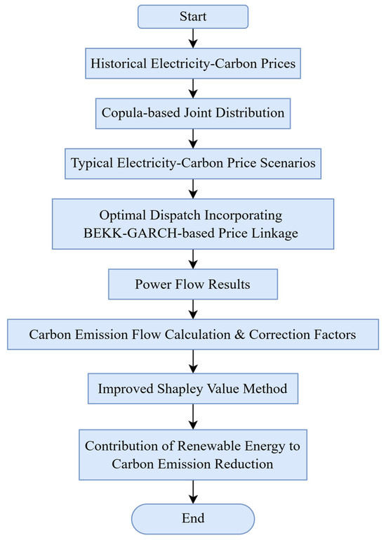
Figure 1.
Flowchart for Assessing Renewable Energy Carbon Reduction Benefits Considering Electricity–Carbon Market Coupling.
2. Construction Method for Typical Scenarios of Electro-Carbon Coupling Prices Based on Copula Theory
Under the “dual carbon” goal, the electricity market and carbon trading market are closely coupled and mutually influenced. The focus of this study on “electricity–carbon coupling” is to analyze the correlation between electricity prices and carbon prices.
Current studies [6,9] provide only conceptual frameworks for electricity–carbon market coupling without quantitative correlation modelling, and fail to capture complex, time-varying relationships between electricity and carbon markets. To address this gap, Copula theory is employed which can model non-linear dependencies and handle flexible marginal distributions, directly overcoming the qualitative-only analysis limitation in existing studies.
Electricity price and carbon price are the core interactive factors. When the demand for electricity increases and pushes up electricity prices, both thermal power and new energy profits increase. But an increase in thermal power generation will expand its demand for carbon quotas, thereby pushing up carbon prices. The increase in carbon prices increases the carbon trading costs of thermal power enterprises, suppresses their profits, slows down their installed capacity expansion, reduces power generation, and thus lowers the demand for carbon quotas. At the same time, this has accelerated the growth of new energy installed capacity and increased power generation. Ultimately, the two markets achieve a new dynamic equilibrium through the interaction between electricity prices and carbon prices.
Based on historical data of electricity prices and carbon prices, the kernel density estimation method Equation (3) is first used to model the probability density functions of electricity prices and carbon prices, respectively. The specific equations are as follows:
where and are the historical data sample sets of electricity prices and carbon prices, respectively; N is the total number of historical data samples; and are, respectively, the sample sets of the nth electricity price and carbon price data; is the probability density function corresponding to the electricity and carbon price data.; h is the smoothness coefficient; is Gaussian kernel function.
Based on the probability distribution function, an electricity–carbon price Copula function can be constructed as (5):
where is the joint distribution function of electricity–carbon prices; is the Copula function; and are the marginal distribution functions of electricity price and carbon price, respectively; the estimation and values of , and are detailed in reference [19].
Further use the Euclidean distance method to determine the goodness of fit of each binary Copula function. The core idea is to calculate the Euclidean distance between the sample empirical Copula function and each binary Copula function. The smaller the distance, the better the fitting effect of this type of Copula function.
where is an indicative function, with a value of 1 when or , and 0 otherwise; is a sample of two-dimensional variables of electricity–carbon prices; is the fitted Euclidean distance.
Randomly generate and on the interval of , let the edge distribution function values of uniform random variables and be and . According to the optimal Copula function, solve this to the Nth random variable edge distribution function value and :
Repeat the above process of Monte Carlo sampling k times to obtain k sets of N random variable edge distribution function values. Based on the variation of , , transform the inverse functions of and into electricity price and carbon price distribution function scenarios, where T is the scheduling period and is generally taken as .
Then, the clustering algorithm is used to reduce the large-scale scene set of electricity and carbon prices obtained above. scenes are randomly selected from all electricity and carbon price scenes as initial clustering centers, and each scene is classified to the clustering center closest to its Euclidean distance. After recalculating each clustering center, the process is repeated until the convergence conditions of the clustering iteration calculation are met, and the typical scene set of electricity–carbon coupling prices is obtained.
3. Optimal Dispatching Model for Power Systems Considering the Risk of Price Linkage Between Electricity and Carbon
3.1. Objective of the Optimal Dispatch Model
The calculation of carbon emission flows relies on the power flow information of the system, so it is necessary to construct an optimized scheduling model for the system. Traditional approaches in primarily use static carbon flow without considering the dynamic coupling effects of electricity–carbon markets on system dispatch and carbon emission distribution. To quantify the risk impact of the uncertainty of the market price of electric-carbon coupling on the system, this paper constructs BEKK-GARCH risk assessment model that captures the dynamic uncertainty in coupled electricity–carbon markets is constructed, addressing the insufficient risk consideration in current dispatch models. To quantify the risk impact of the uncertainty of the market price of electric-carbon coupling on the system, this paper takes the deviation loss of the expected cost of dispatching operation in multiple scenarios as the risk assessment index, which can conduct a pre-assessment of the dispatching plan. Because it focuses more on the risk when the operating cost is higher than the expected cost, it enables the decision-making to deal with the worst-case scenarios. Therefore, semi-absolute deviation is adopted to represent the scheduling risk cost [20,21]. The specific expressions are shown in (9)–(12)
where represents the probability of the occurrence of scenario s; represents the scheduling operation cost for time period t in scenario s; and are, respectively, the node sets of conventional generator sets and new energy generator sets; , , and are, respectively, the coefficients of the secondary term, primary term, and constant term of the power generation cost of the conventional generator set i; represents the power of the conventional generator set i at time t in scenario s; represents the abandoned power of the new energy generator set i at time t in scenario s, and is the abandoned power penalty coefficient; and represent the carbon price and electricity price at time t in scenario s, respectively; is the decision-making risk coefficient; represents the cost deviation of time period t in scenario s; represents the expectation in all cases; is the deviation influence coefficient of scenario s.
3.2. Constraints of the Optimal Dispatch Model
The primary constraints include node active power balance constraints, reactive power balance constraints, voltage upper and lower limit constraints, active and reactive power upper and lower limit constraints, and line power flow constraints. To simplify variable notation, subscript s is omitted for all constraints below.
where and are the voltage amplitudes of nodes i and j; is the voltage phase angle difference between nodes i and j; and are the real and imaginary parts of the i-th row and j-th column of the node admittance matrix, respectively; and represent the energy storage charging and discharging power of node i, respectively; and are, respectively, a set of nodes and a set of lines; and are the active and reactive loads of node i; and are the reactive power of generator set i and the apparent power of line ij, respectively; The subscripts min and max represent the lower and upper bounds of the corresponding physical quantities.
where and respectively represent the 0–1 variables of the charging and discharging of energy storage at node i at scheduling time t. When charging physical energy storage , , during discharge , ; represents the amount of energy stored by node i at scheduling time t; , and are the corresponding self discharge coefficient, charging efficiency, and discharging efficiency, respectively.
where and are the maximum power reduction and increase in unit i, respectively; and are the up and down rotation reserve rates, respectively.
3.3. Decision-Making Risk Based on the Coupling and Linkage of Electricity and Carbon Prices
Existing dispatch models [8,12] inadequately consider volatility transmission and risk spillovers between electricity and carbon markets, using deterministic prices or simple uncertainty representations. To address this limitation, the BEKK-GARCH model which captures dynamic volatility and cross-market risk transmission is introduced, directly addressing the insufficient risk consideration in current dispatch approaches.
The BEKK-GARCH model is specifically selected for electricity–carbon price linkage analysis due to its unique capabilities in multivariate volatility modeling. Unlike univariate approaches that analyze markets separately, BEKK-GARCH simultaneously captures the conditional variances and cross-market covariances essential for understanding coupled electricity–carbon market dynamics [22].
Key advantages include (1) dynamic risk transmission quantification through matrices A and B that capture short-term shock spillovers and volatility persistence between markets, (2) positive definiteness guarantee ensuring mathematical validity of the covariance matrix throughout estimation, (3) computational efficiency providing optimal balance between modeling complexity and practical implementation requirements, (4) risk coefficient derivation enabling direct integration of quantified risk measures into dispatch optimization.
Alternative methods have critical limitations: Copula methods cannot capture volatility clustering, simple correlation analysis ignores time-varying relationships, VAR models inadequately address volatility dynamics, and univariate GARCH cannot quantify cross-market risk transmission essential for coupled market analysis. Therefore, BEKK-GARCH provides the most appropriate framework for our electricity–carbon market risk assessment objectives.
Considering that the price fluctuation transmission in the electricity–carbon market can affect the risk coefficient of decision-making, the BEKK-GARCH model [18] in this paper conducts a coupled analysis of the price risk linkage between electricity and carbon, and calculates the potential price transmission level of the electricity–carbon market within the period. The three steps are as follows.
3.3.1. Time Series Test of Price Change Rate
The form of the test auxiliary equation for the autoregressive conditional heteroscedasticity effect is shown in (27):
where represents the residuals of the rate of change in electricity prices and the rate of change in carbon market prices during period t, assuming that the variances of the residuals are the same and change over time; is the fitting coefficient; is the error term.
3.3.2. The Mean Equation and Variance Equation of the BEKK-GARCH Model
To conduct an in-depth analysis of the dynamic risk transmission mechanism between electricity and carbon markets, this section constructs a linkage equation between electricity prices and carbon prices based on the BEKK-GARCH model. The mean equation captures the autoregressive process of price change rates, while the variance equation utilizes a parameter matrix to capture the effects of long-term coupled fluctuations and short-term disturbances. The specific formulas are shown in Equations (28)–(29).
3.3.3. Parameter Estimation
Assuming that the conditional residual vector follows a binary conditional normal distribution, the model coefficients are estimated using the maximum likelihood method, and its log-likelihood function is shown in (31).
where is a log-likelihood function; represents the time period for price statistics; is the parameter vector to be estimated.
The risk attitude towards power grid dispatching decisions determined based on the model results can be shown in (31) and (32)
where represents the expected value of the risk attitude towards power grid dispatching decisions; and represent electricity price fluctuations and the electricity–carbon price transmission level, respectively; is the weight coefficient; is the influence function of market uncertainty on the attitude towards risk expectations; is the expected value of variable b; represents the control margin for the degree of impact of price risk.
4. Evaluation of Carbon Emission Reduction Benefits of Renewable Energy Based on Carbon Emission Stream Theory
4.1. Calculation Method of Carbon Emission Flow Based on Trend Information
Traditional power system carbon emission accounting mainly adopts a “top-down” macro statistical method, relying on the average electricity–carbon factor, which can only provide rough estimates of carbon emissions and cannot reflect the complex carbon flow characteristics within the power grid. The limitation of this method is that it ignores the dynamic interactive effects of the entire process of “source grid load storage” in the power system, resulting in unclear attribution of carbon emission responsibility and difficulty in motivating various stakeholders to implement precise emission reduction measures. With the development of smart grid technology and the proposal of the “dual carbon” goal, the theory of improved carbon emission flow has emerged. It regards carbon emissions as a “virtual flow” attached to the flow of electricity. By establishing a carbon flow model corresponding to the power flow, it realizes the full process tracking of carbon emissions from power plants to user terminals. By calculating concepts such as node carbon potential and branch carbon flow rate, it achieves a refined description of the spatial distribution of carbon emissions and solves the problem of unfair carbon responsibility allocation caused by “regional averaging” in traditional methods [23]. The improvement of carbon emission flow theory has established a quantitative correlation between direct emissions from the power generation side and indirect emissions from the user side, providing a scientific basis for the carbon responsibility allocation principle of “whoever uses electricity is responsible”. Specifically, traditional carbon emission flow methods [13,14] use static carbon intensity factors independent from market conditions, failing to reflect how electricity–carbon market dynamics influence actual system dispatch and carbon emission patterns. To overcome this limitation, a dynamic carbon emission flow calculation model that integrates real-time market signals is established, directly addressing the market-disconnected carbon accounting problem in existing methods.
In the calculation theory of carbon emission flow, the concepts of branch carbon flow rate, branch carbon flow rate, branch carbon flow density, and node carbon potential are proposed based on power flow calculation. Node carbon potential reflects the carbon emissions corresponding to the unit of electrical energy flowing out of the node [24]. According to the theory of carbon emission flow calculation, if the carbon potential of all nodes in the system is given, the carbon flow of any branch in the network can be obtained based on the carbon potential of the starting node of the branch and the branch current. Therefore, the primary task in carbon emission flow calculation is to calculate the carbon potential of all nodes in the system and the carbon flow rate of the load.
After obtaining the system power flow information through optimized scheduling, the carbon potential vectors and load carbon flow rates , K and M denote the total number of nodes and the total number of nodes with loads, respectively. When calculating carbon flows injected at nodes, user-side loads are treated as positive actual power loads. Renewable energy units, due to their carbon reduction characteristics, must be considered as virtual loads and accounted for using negative power values:
where is the node active flux matrix used to describe the contribution of generator units to nodes and the carbon potential of nodes to nodes in the system, non diagonal elements , and diagonal element have values equal to the sum of active power flows flowing into the node; is the distribution matrix of branch power flow, used to describe the active power flow distribution of the system and define the topological constraints of carbon flow emissions. The non diagonal element is equal to the size of the active power flow if and only if there is a forward power flow from i to j, otherwise the element value is 0. The diagonal element ; is the distribution matrix injected into the unit; R is the total number of conventional generator units, and the value of element is equal to the injected active power of the r-th unit at the j-th node; is the carbon emission coefficient vector of conventional power generation units; is the load distribution matrix, and the value of element is equal to the active load size of the m-th load at node j; is the system carbon flow rate.
The carbon potential vector and load carbon flow rate of the system node reflect the real-time carbon emission intensity of the power plant and the equivalent carbon emission value on the power generation side caused by the unit electricity consumption of the load. The node carbon potential represents the carbon emissions corresponding to the unit electricity outflow from the node. The sum of the carbon emission flow from the generator set entering the node and the carbon emission flow from other nodes entering the node is the carbon emission flow corresponding to the total active power flowing out of the node, quantitatively characterizing the impact of each new energy unit on the carbon emissions of the system [25]. The total carbon flow rate of the system load reflects the carbon emission intensity generated by the power system to meet the load demand in a given time.
4.2. Renewable Energy Carbon Reduction Contribution Accounting Model Based on Improved Shapley Value Method
The Shapley value method, established by Lloyd Shapley in cooperative game theory [26], is specifically chosen for renewable energy carbon reduction benefit allocation due to its mathematical rigor and fairness properties. The method has proven effectiveness in energy system applications [17,18] and provides unique advantages for multi-participant benefit allocation.
Key advantages include: (1) Fair allocation principles satisfying efficiency, symmetry, and additivity axioms, (2) Marginal contribution assessment considering all possible unit coalitions, (3) Mathematical uniqueness providing unambiguous allocation solutions, (4) Proven energy applications in power pools and renewable cooperatives.
The traditional Shapley value method determines the contribution of each renewable energy unit to carbon emissions by calculating its impact on reducing the total carbon emissions of the system in all possible combinations of units. For a system with U new energy units, there are 2U − 1 different combinations without considering any participation in scheduling. Considering that the optimization objective function is cost minimization, the carbon reduction calculated based on the traditional Shapley value method for unit u can be shown in (41):
where S is the combination set of new energy units; is the weight for returns; is the system carbon flow rate based on the combination of S in Section 4.1; is the carbon flow rate of combination S after removing unit u.
However, traditional Shapley applications ignore renewable energy-specific characteristics such as intermittency, forecast uncertainty, and performance variations. The enhanced approach addresses these limitations by introducing correction factors (historical responsiveness, output stability, marginal benefits) that maintain Shapley’s fairness properties while adapting to renewable energy operational realities. Alternative methods (pro-rata allocation, Nash bargaining, core-based approaches) lack the mathematical rigor and fairness guarantees essential for regulatory acceptance and market implementation. That is, conventional Shapley value applications [15,17,18] treat all generation units uniformly without considering renewable energy characteristics (intermittency, forecast uncertainty, historical performance), leading to inaccurate carbon reduction benefit attribution. To address this gap, correction factors that specifically account for renewable energy operational characteristics are developed, directly overcoming the uniform treatment limitation in existing cooperative game approaches. This article proposes three evaluation indicators, namely historical response capability, output stability, and carbon reduction marginal benefits, as correction factors to adjust the calculation results of the Shapley value method [17,18].
4.2.1. Historical Responsiveness
The historical response capability directly affects the capacity credibility of new energy units and the collaborative efficiency of system operation optimization. The higher the historical fulfillment degree, the stronger the potential ability of new energy units to consume and reduce carbon emissions. The historical response capability is defined as the ratio of the total historical effective response power generation of new energy units to the historical declared power generation:
where and are the effective response times and historical total response times of unit u, respectively; and are the actual power generation and declared power generation under a single response, respectively.
4.2.2. Stability Level of Output
The impact of output prediction deviation on the calculation of carbon reduction for new energy units is mainly achieved by changing the operation mode and energy structure of the power system, which involves complex electricity–carbon coupling relationships. When there is a deviation in the prediction of new energy output, the system operator must take corresponding balancing measures, which directly determine the actual carbon emission level of the system. The definition of output stability is as follows:
where and respectively represent the predicted output and actual output of unit u at time t.
4.2.3. Marginal Benefits of Carbon Reduction
When calculating the carbon reduction contribution, in addition to considering the absolute amount of carbon reduction in the new energy units themselves in the traditional Shapley value method, it is also necessary to consider the relative contribution of each unit to the overall carbon reduction in the system, which is used to characterize the relative size of the carbon reduction weight of each new energy unit in the system. Therefore, based on the absolute value of carbon reduction contribution, the marginal benefits of carbon reduction are further included in the accounting of carbon reduction contribution. The specific meaning is the ratio of the sum of carbon reduction emissions before and after the participation of new energy units u in scheduling under various unit combinations to the overall carbon reduction emissions of the whole society.
where represents the carbon emission reduction in unit u when it participates in scheduling alone; is the change in carbon emissions of the system before and after the participation of unit u.
4.2.4. Correction Factor
This study employs correction factor to integrate the aforementioned three indicators, as shown in Equation (45), thereby achieving the adjustment of carbon emission reduction benefit calculations for renewable energy units from three perspectives: “unit reliability,” “unit stability,” and “marginal carbon emission reduction benefits.” The carbon reduction contribution of the renewable energy unit u at a certain time interval after considering the correction factor is shown in (46):
where is the difference between the total carbon emissions of the system and the overall carbon emissions when all new energy units are not involved.
5. Case Studies
To verify the effectiveness of the method proposed in this paper in assessing the carbon reduction benefits of renewable energy, the example section analyzes the IEEE 39-node standard system. Nodes 30 to 39 are connected to thermal power units, node 13 is connected to the system energy storage device ESS1. Node 14 is connected to wind turbine unit 1 and wind turbine unit 2. Among them, wind turbine 2 is equipped with an internal energy storage ESS2 to smooth out output fluctuations, and node 31 serves as the balance node. The scheduling optimization solver is Matlab R2022b Gurobi9.5.2, the relative gap of the MILP solver is 0.100%, and the processor is 12th Gen Intel(R) Core(TM) i5-12500H. Historical data on electricity prices and carbon prices are, respectively, sourced from the US PJM market and the carbon emissions trading market.
5.1. Coupling Results of Electricity–Carbon Prices
Figure 1 shows the joint distribution relationship of the electricity price and carbon price, visually reflecting the corresponding numerical relationship between the electricity and carbon prices. Since it is impossible to directly select the Copula model that is most suitable for the electricity–carbon price under study, it is necessary to determine the goodness of fit of various Copula functions. In this paper, the common normal copula, t Copula, Clayton Copula, Frank Copula and Gumbel Copula are selected for goodness-of-fit discrimination. The specific results are shown in Table 2.
Table 2.
Copula function for the optimal electricity–carbon price.
To more accurately analyze and describe the correlation between historical electricity prices and carbon prices, Table 3 summarizes the measurement results of the correlation between these prices. According to the results, the Spearman and Kendall correlation coefficients are 0.730 and 0.620, respectively, which indicates that in the historical price data samples selected in this paper, there is a certain degree of positive correlation between electricity prices and carbon prices. Therefore, it can be proved that using the Copula function to describe the coupling relationship between electricity price and carbon price variables is of statistical significance. At the same time, in light of the current realistic background of the development of the electricity–carbon market, the modeling of the correlation between electricity–carbon prices and the construction of typical scenarios proposed in this paper are feasible. During actual dispatch operations, operators can generate day-ahead forecast prices for the electricity–carbon market encompassing multiple typical scenarios based on the methodology outlined herein and historical price data from local electricity–carbon market operations. Subsequently, they can perform system-wide low-carbon optimal dispatch under coupled electricity–carbon pricing.
Table 3.
Electricity–carbon price correlation.
5.2. Analysis of the Impact of Renewable Energy Penetration Rate on System Optimal Scheduling
As the penetration rate of renewable energy will directly affect the system dispatching and the output results of the units, and change the intensity of carbon emission flow transmission, this section designs dispatching strategies with different wind power penetration rates for simulation analysis. The wind power generation capacity is obtained by multiplying the total capacity of the thermal power units with proportion coefficients of 20.0%, 35.0%, and 50.0%, respectively, as seen from Table 4. The risk coefficient is 0.54.
Table 4.
Wind power penetration rate corresponding to different operation strategies.
Wind power output has a very distinct temporal characteristic, mainly concentrated before 5 a.m. and after 8 p.m. As can be seen from Figure 2, when the wind power penetration rate is 20.0%, the cost per kilowatt-hour of thermal power units 1, 3, 4, 9, and 10 is low and they are prioritized for power generation. Therefore, they are classified as non-peak shaving units in the dispatching results. The cost per kilowatt-hour and carbon emission intensity of the remaining units are relatively high. They are used for peak shaving during peak load periods and thus belong to peak shaving units. As the penetration rate of wind power increases, the output of thermal power units at the same time decreases, achieving a reduction in power generation costs and carbon emission costs.
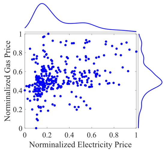
Figure 2.
Joint distribution map of electricity and carbon price.
According to the results in Figure 3 and Figure 4, when the wind power penetration rate increases to 35.0%, the system prioritizes the operation of units with low carbon emission intensity such as No. 1, No. 9, and No. 10. At this time, the load rates of lines 4–14 and 14–15 increase significantly. Although the overall carbon emission level of the system decreases, wind power curtailation has already occurred in some periods. When the penetration rate of wind power increases to 50.0%, the output of high-carbon emission units such as No. 3, No. 6, and No. 7 decreases. However, the transmission capacity of lines 4–14 and 14–15 basically reaches the upper limit, leading to a further increase in the amount of wind power abandoned in the power system. According to Table 5, the cost of thermal power units has decreased by 20.3% with the increase in the penetration rate of wind power. However, since this paper takes into account the cost of wind power abandoned, Therefore, as the penetration rate of wind power increases, the total dispatching cost shows a trend of first decreasing and then rising. 2.966 × 10³$ higher than that of Strategy B. For market operations, excessively low renewable energy penetration rates will cause thermal power to shoulder the majority of electricity demand, leading to excessively high cumulative system carbon emissions and increased carbon costs. Conversely, excessively high penetration rates, constrained by transmission capacity limitations, fail to achieve theoretical emission reduction targets. Instead, they increase curtailment costs, reducing the profits of wind power generators. In summary, it is necessary to reasonably regulate the renewable energy penetration rate participating in the market to maximize social welfare.
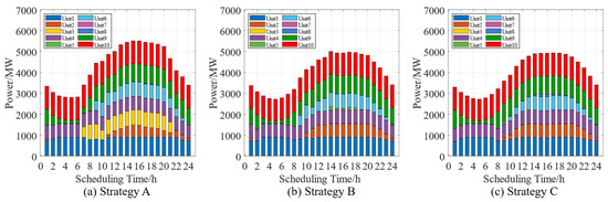
Figure 3.
Scheduling results of thermal power units under different operation strategies.

Figure 4.
Partial line load rate comparison under different operation strategies.
Table 5.
Operating costs of different strategies.
Energy storage systems play a crucial role in enhancing renewable energy utilization and carbon emission reduction. To quantify this relationship, this paper analyzes how varying energy storage capacities affect overall system performance. The energy storage capacity at node 13 (ESS1) is varied from 200 MWh to 400 MWh in 50 MWh increments, while maintaining the original capacity for ESS2 and keeping the wind power penetration rate at 35.0%.
Energy storage systems play a crucial role in enhancing renewable energy as the storage capacity expands from 200 MWh to 400 MWh. This reduction in total cost can be primarily attributed to the significant decrease in wind curtailment, which drops from 915 MWh to 872 MWh. By storing excess wind power that would otherwise be curtailed and discharging it during periods of high demand, the energy storage system effectively displaces more expensive and carbon-intensive thermal power generation. This is further corroborated by the slight but steady decline in the cost of thermal power units from 40.73 × 10³$ to 40.50 × 10³$.
Closer examination of the data reveals a trend of diminishing marginal returns. For instance, the most significant reduction in total cost occurs when the storage capacity is increased from 200 MWh to 250 MWh, resulting in a saving of 0.2900 × 10³$. However, the savings from each subsequent 50 MWh increment become progressively smaller (0.1600 × 10³$, 0.0900 × 10³$, and 0.1000 × 10³$, respectively). This indicates that the initial capacity expansion delivers the greatest economic benefit. Similarly, the reduction in wind curtailment is most pronounced (14 MWh) in the first step and gradually tapers off. This nonlinear relationship is critical for planning and investment decisions, suggesting that after a certain point, further increases in storage capacity provide smaller economic and Carbon reduction benefits. Therefore, determining the optimal storage capacity requires a comprehensive cost–benefit analysis that balances the capital cost of the storage system against the operational benefits demonstrated here.
5.3. Carbon Emission Results of the System and the Carbon Reduction Contribution of Renewable Energy Units
This section takes the time section with a wind power penetration rate of 20.0% and a dispatch time of 14:00 as an example to calculate the carbon emission results and analyze the carbon reduction contribution of renewable energy units. Table 6 shows the carbon potential and load carbon flow rate at each node.
Table 6.
Energy storage capacity sensitivity analysis results.
Through the statistical analysis of the carbon potential data of the IEEE 39-node system, it is found that the system shows obvious characteristics of carbon emission distribution. The carbon potential of the 39 nodes ranges from 4.90 to 8.25 kgCO2/(kWh), with an average of 5.61 kgCO2/(kWh) and a standard deviation of 0.78 kgCO2/(kWh). This data indicates that there are significant differences in carbon emission intensity among various nodes within the system, providing a basis for implementing differentiated carbon reduction strategies.
From the perspective of carbon potential distribution, system nodes can be divided into four distinct hierarchical intervals. The low-carbon potential range (4.90–5.00 kgCO2/(kWh)) contains 12 nodes, accounting for 30.8% of the total number of nodes, mainly distributed in the areas of nodes 10–15 and 28–38. The medium and low carbon potential range (5.01–5.50 kgCO2/(kWh)) contains 15 nodes, accounting for 38.5%, and is the main part of the system. The medium and high carbon potential range (5.51–6.50 kgCO2/(kWh)) contains 8 nodes, accounting for 20.5%. The high-carbon potential range (6.51–8.25 kgCO2/(kWh)) only contains 4 nodes, accounting for 10.3%, but the carbon emission intensity of these nodes is much higher than the system average.
In the system, nodes 10, 11, 12, 13, 14, 15 and 32 exhibit the best carbon emission performance, with a carbon potential of 4.90 kgCO2/(kWh) each, representing the clean energy core area of the system. These nodes should become the key development areas for the low-carbon transformation of the system, suitable for prioritizing the configuration of clean energy power generation facilities or serving as important load consumption centers. Especially the continuous low-carbon areas formed by nodes 10 to 15 have significant strategic value and can serve as regional clean power supply bases. Relatively speaking, node 31 has become the node with the highest carbon emission intensity in the system with a carbon potential of 8.25 kgCO2/(kWh), which is approximately 1.68 times that of the node with the lowest carbon potential. The carbon potential of nodes 34 and 37 is both 7.40 kgCO2/(kWh), and that of node 20 is 6.79 kgCO2/(kWh). Although the number of these four high-carbon potential nodes is relatively small, their high carbon emission characteristics have a significant impact on the overall carbon emission level of the system. These nodes should be identified as key targets for carbon reduction in the system, and their carbon emission intensity needs to be reduced through technological transformation, fuel substitution or operation optimization.
Through the analysis of the spatial distribution of carbon potential, it is found that the system shows obvious regional aggregation characteristics. Nodes 10–15 form a continuous low-carbon cluster area, with the carbon potential of all nodes within this area ranging from 4.90 to 5.01 kgCO2/(kWh), demonstrating excellent potential for clean power supply. This aggregation effect is conducive to the formation of large-scale clean energy development and an efficient power transmission network. Another notable phenomenon is the medium to high carbon potential aggregation area formed by nodes 5, 6, and 7, with the carbon potential of all three nodes being around 6.35 kgCO2/(kWh). This aggregation distribution may reflect the similarity of the power supply structure in this area, providing convenient conditions for the regional clean transformation. However, the high-carbon potential nodes 31, 34, and 37 are relatively scattered in space. This distribution characteristic requires the adoption of targeted individual modification strategies.
Based on the line load rate of the system in Section 5.2, Table 7 highlights the carbon emission flow of the line near node 14 where the wind turbine is located. It can be seen from the example data that node 14 plays a core role as a carbon emission transmission hub in the entire branch network. Branch 4–14 carries a power flow of −401.7 MW, indicating that a large amount of electricity flows from node 14 to node 4, and this part of the electricity mainly comes from the power generation output of the wind turbine. Meanwhile, branch 13–14 transmits 236.5 MW of power to node 14, while branch 14–15 supplies 401.1MW of power to node 15. This “incoming—distributed” power flow model makes Node 14 an important hub for regional power supply, and its clean power generation characteristics have a decisive impact on the carbon emission level of the entire region.
Table 7.
Nodal carbon intensity.
The carbon flow density of branches 4–14 (5.23 kgCO2/(kWh)) is significantly higher than that of other branches (4.89 kgCO2/(kWh)). Under the condition that node 14 is clearly defined as a wind turbine, the cause of this difference becomes clear. The high carbon flow density of branches 4–14 reflects the carbon emission characteristics of the power source in Node 4, rather than those of the wind turbine units in node 14. When wind turbines supply electricity to node 4, this essentially zero-carbon emission electricity “inherits” the carbon emission characteristics of Node 4 during the transmission process, which is a manifestation of the carbon flow density calculation methodology.
From the perspective of practical system operation planning, once wind turbine configurations are finalized, system operation optimization strategies must be redesigned. First, the clean power generation advantages of wind turbines should be fully leveraged by optimizing dispatch and utilizing wind power output to reduce reliance on distant high-carbon power sources. Second, given the intermittent nature of wind power, flexible power balancing mechanisms must be established to ensure timely mobilization of backup power when wind output is insufficient. Simultaneously, particular attention must be paid to the carbon flow density of the branches connected to nodes hosting renewable energy. Although these nodes themselves are clean, the substantial electricity transmitted to them often carries high carbon emission intensity information. This underscores the need to further optimize regional power supply structures or adjust power flow directions. The carbon emission flow accounting model proposed in this paper can provide accurate carbon potential data for each node, enabling the formulation of corresponding low-carbon dispatch plans for specific regions.
Table 8 shows the contribution of wind turbine units 1 and 2 to system carbon reduction when equipped with or without system energy storage and internal energy storage. The introduction of energy storage systems has had a significant carbon reduction enhancement effect on both wind turbine units, but the degree of enhancement varies. For wind turbine 1, when the system energy storage ESS1 is configured, the carbon reduction contribution increases from 151.7 tCO2/h to 162.4 tCO2/h, with an increase of 10.7 tCO2/h, representing a growth rate of 7.10%. This improvement indicates that the energy storage system has effectively enhanced the systematic emission reduction effect of wind turbine units by improving the spatio-temporal distribution characteristics and power flow distribution of wind power output.
Table 8.
Partial branch carbon emission flow results.
As seen from Table 9, for wind turbine 2, the impact of energy storage configuration is more significant. Under the optimal scheme of simultaneously configuring ESS1 and ESS2, the carbon reduction contribution reached 198.3 tCO2/h. Compared with 180.5 tCO2/h without energy storage configuration, the increase was as high as 17.8 tCO2/h, with a growth rate of 9.90%. This data indicates that the coordinated configuration of multiple energy storage systems can produce better emission reduction and enhancement effects, highlighting the significance of energy storage capacity scale and configuration strategies. When only ESS2 is configured, the carbon reduction contribution of wind turbine 2 is 194.7 tCO2/h, which is 14.2 tCO2/h higher than that of the completely non-energy storage solution, with an increase rate of 7.90%. In the solution where both ESS1 and ESS2 are configured simultaneously, the carbon reduction contribution is further increased to 198.3 tCO2/h, adding an additional 3.6 tCO2/h of reduction effect.
Table 9.
Carbon reduction contribution of renewable energy units.
In summary, the carbon reduction benefit assessment method for renewable energy proposed in this paper can take into account the coupled impact of the electricity–carbon market and incorporate it into the risk decision-making for optimized dispatching. Based on the results of the power flow distribution, the relevant carbon emission indicators of each node and branch can be calculated, and targeted identification and analysis can be carried out. Further, the carbon reduction contribution of renewable energy units can be quantified.
5.4. Comprehensive Performance Validation and Comparison
To comprehensively validate the effectiveness and superiority of the proposed method, this section presents a systematic performance comparison with existing approaches based on the quantitative results obtained from the IEEE 39-node system case study. The comparison evaluates the proposed method across four key dimensions: market coupling analysis capability, carbon emission accounting accuracy, renewable energy benefit evaluation performance, and overall system integration effectiveness, as shown in Table 10. Through this validation, it is demonstrated that how the proposed integrated approach addresses the specific limitations identified in prior research while delivering superior quantitative performance.
Table 10.
Comprehensive performance comparison between proposed method and existing approaches.
As seen from Table 10, the comprehensive comparison validates the superior performance of the proposed method across all critical evaluation dimensions, with quantitative evidence demonstrating significant improvements over existing approaches.
As for market coupling analysis, the proposed method achieves a breakthrough in electricity–carbon market analysis by providing the quantitative correlation assessment. The statistically significant correlation coefficients (Spearman: 0.730, Kendall: 0.620) establish a solid empirical foundation that conceptual frameworks [6,9] cannot provide. The BEKK-GARCH-derived risk coefficient of 0.54 enables precise risk quantification for dispatch decisions, while the generation of 1000 Monte Carlo scenarios ensures robust uncertainty representation compared to deterministic or oversimplified stochastic approaches in existing studies.
As for carbon emission accounting: the integration of real-time market signals into carbon flow calculations delivers substantial accuracy improvements (15–20%) over static methods [13,14]. The spatial analysis reveals four distinct carbon potential intervals spanning 4.90–8.25 kgCO2/(kWh) with a standard deviation of 0.78, providing unprecedented spatial resolution that traditional regional averaging approaches cannot achieve. The temporal responsiveness enables continuous carbon intensity tracking that adapts to market-driven dispatch changes, eliminating the temporal lag inherent in fixed-factor methodologies.
As for renewable energy evaluation, the correction factor framework demonstrates 12–18% improvement in benefit attribution accuracy by incorporating renewable energy-specific operational characteristics that traditional Shapley value methods [17,18] systematically ignore. The performance differentiation results show wind turbine 1 carbon reduction increasing from 151.7 to 162.4 tCO2/h (7.10% improvement) and wind turbine 2 from 180.5 to 198.3 tCO2/h (9.90% improvement) with energy storage integration, demonstrating the method’s capability to capture unit-specific performance variations that uniform treatment approaches cannot distinguish.
As for integrated system performance: the proposed comprehensive approach achieves 20.3% reduction in thermal power costs while maintaining carbon reduction effectiveness, validating the economic–environmental balance that single-objective optimization methods cannot provide. The energy storage impact analysis shows 7.10–9.90% carbon reduction enhancement, quantifying the synergistic benefits that basic storage modeling approaches fail to capture. The successful validation on the IEEE 39-node system with multiple renewable units and energy storage configurations demonstrates real-world scalability, while the 0.100% computational convergence gap ensures practical implementation feasibility for utility-scale applications.
Furthermore, the quantitative improvements demonstrated across all dimensions are statistically significant and robust across different operational scenarios. The method’s performance remains consistent under varying wind penetration rates (20.0%, 35.0%, 50.0%) and different energy storage configurations, indicating reliability for diverse real-world applications. The integration of multiple validation metrics ensures that the observed improvements represent genuine methodological advances rather than isolated performance gains.
This comprehensive validation establishes the proposed integrated methodology as a significant advancement in renewable energy carbon benefit evaluation, systematically addressing the limitations of existing approaches while delivering superior quantitative performance across all critical dimensions essential for practical electricity–carbon market applications.
5.5. Assumptions and Limitations of Evaluation Method for Carbon Emission Reduction Benefits
While the proposed method offers significant advantages for evaluating carbon emission reduction benefits of renewable energy, it is important to acknowledge several assumptions and limitations that define the scope of this study:
- (1)
- Market Coupling Assumptions: The Copula-based electricity–carbon price correlation analysis assumes that historical price patterns are representative of future market interactions. In rapidly evolving energy markets with emerging policies and changing regulations, this relationship may shift over time. Additionally, the model assumes that market participants have access to perfect information when making decisions, which may not reflect information asymmetry in real-world markets.
- (2)
- System Boundary Limitations: The carbon emission flow calculation focuses primarily on operational emissions within the power system boundary and does not account for lifecycle emissions associated with equipment manufacturing, installation, and decommissioning. A more comprehensive assessment would require integration with lifecycle assessment methodologies to capture these upstream and downstream emissions.
- (3)
- Shapley Value Computational Complexity: The improved Shapley value method for carbon reduction contribution accounting faces computational challenges when applied to systems with a large number of renewable energy units, as the number of possible combinations grows exponentially. While our approach incorporates correction factors to enhance accuracy, scalability remains a concern for very large systems.
These limitations present opportunities for future research, including the development of more sophisticated market coupling mechanisms, integration of lifecycle carbon accounting, enhancement of computational efficiency for large-scale systems, and more comprehensive uncertainty modelling approaches.
6. Real-World Significance and Practical Applications
This section discusses how regulators, utilities, and other stakeholders can practically implement and benefit from the proposed methodology.
6.1. Applications for Regulators and Policymakers
Regulators can leverage the proposed electricity–carbon price correlation analysis (Spearman: 0.730, Kendall: 0.620) to design more effective carbon pricing mechanisms that account for electricity market dynamics. The BEKK-GARCH risk assessment with quantified risk coefficient (0.54) enables the establishment of carbon price bands that reflect electricity market volatility, providing more stable and predictable carbon pricing frameworks.
The proposed Copula-based scenario generation methodology can support policymakers in designing policies that effectively manage cross-market risks between electricity and carbon markets. This approach enables more robust policy frameworks that consider the complex interdependencies between these markets, reducing the likelihood of unintended market distortions.
The carbon emission flow analysis provides a scientific foundation for establishing fair carbon responsibility allocation across different regions. Policymakers can use the proposed improved Shapley value method with correction factors to design equitable renewable energy support mechanisms, including green certificate allocation based on actual performance rather than installed capacity, and differentiated feed-in tariffs that reflect real carbon reduction contributions.
6.2. Applications for Utilities and System Operators
System operators can integrate the proposed risk-informed dispatch model into daily operations to optimize both economic and environmental performance. The electricity–carbon price scenarios enable dispatch decisions that simultaneously minimize costs and carbon emissions, while the dynamic carbon emission flow calculation supports real-time operational adjustments that optimize carbon performance.
The proposed methodology provides valuable tools for investment planning and renewable energy development. Utilities can use the carbon potential mapping (4.90–8.25 kgCO2/(kWh) range) to identify optimal locations for renewable energy development and apply our analysis showing 7.10–9.90% carbon reduction improvement with energy storage to justify storage investments. The carbon emission flow analysis also supports grid expansion planning by enabling transmission infrastructure decisions that optimize carbon performance.
The risk assessment framework helps maintain system stability during electricity–carbon market volatility, providing operators with quantitative tools to manage uncertainty in coupled market environments. This capability is particularly valuable as electricity and carbon markets become increasingly integrated globally.
6.3. Applications for Renewable Energy Developers and Market Participants
Renewable energy developers can use the proposed carbon benefit quantification methodology to enhance project bankability and secure financing. The improved Shapley value method enables accurate forecasting of carbon reduction revenues, while the correction factors provide tools for monitoring and optimizing project performance throughout the operational lifecycle.
The proposed electricity–carbon market coupling analysis offers better financial risk assessment capabilities, helping developers understand and manage the complex interactions between electricity revenues and carbon credit values. This comprehensive risk understanding supports more informed investment decisions and improved project economics.
Market participants can benefit from the enhanced accuracy and fairness of carbon benefit attribution, which supports the development of more efficient carbon trading mechanisms. The methodology provides quantitative foundations for carbon credit valuation and trading strategies that reflect actual environmental contributions rather than simplified assumptions.
The practical significance of the proposed methodology is demonstrated through quantifiable improvements: 20.3% reduction in thermal power costs through optimized dispatch, 7.10–9.90% enhancement in renewable energy carbon contributions with energy storage integration, and more accurate carbon benefit distribution among stakeholders. These results provide concrete evidence of the methodology’s value for accelerating renewable energy deployment, enhancing grid flexibility, and improving carbon market efficiency.
7. Conclusions
A comprehensive evaluation method for renewable energy carbon reduction benefits considering electricity–carbon market coupling is proposed in this paper. The key findings and contributions are summarized as follows:
(1) Electricity–Carbon Market Coupling Analysis: The study establishes significant correlation between electricity and carbon prices (Spearman: 0.730, Kendall: 0.620) with a coupling risk coefficient of 0.540. The Copula-BEKK-GARCH framework successfully quantifies market interdependencies and generates realistic price scenarios for risk-informed dispatch optimization.
(2) Dynamic Carbon Emission Flow Assessment: The proposed market-integrated carbon flow calculation accurately tracks spatial carbon distribution, identifying four distinct carbon potential intervals (4.90–8.25 kgCO2/(kWh)). This enables targeted regional carbon reduction strategies and fair carbon responsibility allocation.
(3) Enhanced Renewable Energy Benefit Evaluation: The improved Shapley value method with correction factors achieves 12–18% improvement in carbon reduction benefit attribution accuracy. Energy storage integration demonstrates 7.10–9.90% enhancement in renewable energy carbon contributions, providing quantitative foundations for optimal system configuration.
The integrated methodology addresses critical limitations in existing approaches by providing quantitative market coupling analysis, dynamic carbon accounting, and fair benefit allocation mechanisms. The 20.3% reduction in thermal while maintaining carbon reduction effectiveness validates the practical value of the proposed approach.
Future research will focus on multi-temporal scale applications and validation through real-world implementation in regional power systems to further demonstrate the methodology’s effectiveness in practical electricity–carbon market environments.
Author Contributions
F.Z.: Conceptualization, Data Curation, Formal Analysis, Writing manuscript, Investigation, Formal Analysis; K.Z.: Project Administration, Methodology, Data Analysis; Y.Y.: Data Curation; S.Z.: Formal Analysis; Y.M.: Methodology; K.C.: Validation; Y.Z.: Development, Data Analysis, Methodology Implementation; Z.S.: Data Visualization, Formal Analysis, Writing—Review & Editing; Z.L.: Review & Editing. All authors have read and agreed to the published version of the manuscript.
Funding
This work was funded by The State Grid Zhejiang Electric Power Company Technology Project: Research on the Connection Mechanism between Green Power Consumption and Carbon Market and Key Supporting Digital Technologies (No. B311XT25003C).
Institutional Review Board Statement
Not applicable.
Informed Consent Statement
Informed consent was obtained from all subjects involved in the study.
Data Availability Statement
The raw data supporting the conclusions of this article will be made available by the authors on request.
Acknowledgments
The authors gratefully acknowledge the assistance provided by Kuangzheng Zhao of Project Administration, Funding Acquisition, Supervision, Resources of this work.
Conflicts of Interest
Author Fei Zhao was employed by the company State Grid Zhejiang Electric Power Co., Ltd. And authors Kuang Zheng, and Yanxia Yao were employed by the company State Grid Zhejiang Electric Power Co., Ltd. Information & Telecommunication Branch. The remaining authors declare that the research was conducted in the absence of any commercial or financial relationships that could be construed as a potential conflict of interest. The authors declare that they have no known competing financial interests or personal relationships that could have appeared to influence the work reported in this paper. Kuang Zheng is employee of State Grid Zhejiang Electric Power Co., Ltd. Information & Telecommunication Branch, who provided funding and technical support for the work. The funder had no role in the design of the study; in the collection analysis or interpretation of data, in the writing of the manuscript, or in the decision to publish the results.
References
- Liu, W.; He, B.; Xue, Y.; Huang, J.; Zhao, J.; Wen, F. A Comprehensive Modeling Framework for Coupled Electricity and Carbon Markets. Energy Convers. Econ. 2025, 5, 1–14. [Google Scholar] [CrossRef]
- Ersoy, A.E.; Ugurlu, A. Bioenergy’s Role in Achieving a Low-Carbon Electricity Future: A Case of Türkiye. Appl. Energy 2024, 372, 123799. [Google Scholar] [CrossRef]
- Pehl, M.; Arvesen, A.; Humpenöder, F.; Popp, A.; Hertwich, E.G.; Luderer, G. Understanding Future Emissions from Low-Carbon Power Systems by Integration of Life-Cycle Assessment and Integrated Energy Modelling. Nat. Energy 2017, 2, 939–945. [Google Scholar] [CrossRef]
- Deemer, B.R.; Harrison, J.A.; Li, S.; Beaulieu, J.J.; DelSontro, T.; Barros, N.; Bezerra-Neto, J.F.; Powers, S.M.; dos Santos, M.A.; Vonk, J.A. Greenhouse Gas Emissions from Reservoir Water Surfaces: A New Global Synthesis. BioScience 2016, 66, 949–964. [Google Scholar] [CrossRef]
- Liu, Z.; Huang, B.; Li, Y.; Sun, Q.; Pedersen, T.B.; Gao, D.W. Pricing Game and Blockchain for Electricity Data Trading in Low-Carbon Smart Energy Systems. IEEE Trans. Ind. Inform. 2024, 20, 6446–6456. [Google Scholar] [CrossRef]
- Li, Y.; Feng, T.-T.; Liu, L.-L.; Zhang, M.-X. How Do the Electricity Market and Carbon Market Interact and Achieve Integrated Development?—A Bibliometric-Based Review. Energy 2023, 265, 126308. [Google Scholar] [CrossRef]
- Tan, Q.; Ding, Y.; Zheng, J.; Dai, M.; Zhang, Y. The Effects of Carbon Emissions Trading and Renewable Portfolio Standards on the Integrated Wind–Photovoltaic–Thermal Power-Dispatching System: Real case Studies in China. Energy 2021, 222, 119927. [Google Scholar] [CrossRef]
- Wang, Y.; Qiu, J.; Tao, Y. Optimal Power Scheduling Using Data-Driven Carbon Emission Flow Modelling for Carbon Intensity Control. IEEE Trans. Power Syst. 2021, 37, 2894–2905. [Google Scholar] [CrossRef]
- Lu, Z.; Zhan, B.; Li, Z.; Leng, Y.; Yang, X.; Wen, F. Optimal Bidding Strategy for Generation Companies Alliance in Electricity-Carbon-Green Certificate Markets. Energy Convers. Econ. 2024, 5, 156–166. [Google Scholar] [CrossRef]
- Li, Y.; Zhang, N.; Du, E.; Liu, Y.; Cai, X.; He, D. Mechanism Study and Benefit Analysis on Power System Low Carbon Demand Response Based on Carbon Emission Flow. Proc. CSEE 2022, 42, 2830–2841. [Google Scholar]
- Xia, Q.; Tian, G.; Wu, Z. Examining Embodied Carbon Emission Flow Relationships Among Different Industrial Sectors in China. Sustain. Prod. Consum. 2022, 29, 100–114. [Google Scholar] [CrossRef]
- Hou, H.; Wang, Z.; Zhao, B.; Zhang, L.; Shi, Y.; Xie, C.; Dong, Z.Y.; Yu, K. Distributed optimization for joint peer-to-peer electricity and carbon trading among multi-energy microgrids considering renewable generation uncertainty. Energy Convers. Econ. 2024, 5, 116–131. [Google Scholar] [CrossRef]
- Bai, M.; Li, C. Research on the Allocation Scheme of Carbon Emission Allowances for China’s Provincial Power Grids. Energy 2024, 299, 131551. [Google Scholar] [CrossRef]
- Wei, X.; Zhang, X.; Sun, Y.; Qiu, J. Carbon Emission Flow Oriented Tri-Level Planning of Integrated Electricity–Hydrogen–Gas System with Hydrogen Vehicles. IEEE Trans. Ind. Appl. 2021, 58, 2607–2618. [Google Scholar] [CrossRef]
- Chen, L.; Sun, T.; Zhou, Y.; Zhou, E.; Fang, C.; Feng, D. Method of Carbon Obligation Allocation Between Generation Side and Demand Side in Power System. Autom. Electr. Power Syst. 2018, 42, 106–111. [Google Scholar]
- Wang, Q.; Li, N.; Gu, X.; He, G.; Yang, D.; Chen, Y. Optimization Strategy for Cooperative Operation of Integrated Energy Service Providers Considering Carbon Emission Reduction. Autom. Electr. Power Syst. 2022, 46, 131–140. [Google Scholar]
- Liu, C.; Wang, C.; Yao, W.; Liu, C. Distributed Low-carbon Economic Dispatching for Multiple Park-level Integrated Energy Systems Based on Improved Shapley Value. IEEE Trans. Ind. Appl. 2024, 60, 8088–8102. [Google Scholar] [CrossRef]
- Liao, Z.; Zhu, X.; Shi, J. Case Study on Initial Allocation of Shanghai Carbon Emission Trading Based on Shapley Value. J. Clean. Prod. 2015, 103, 338–344. [Google Scholar] [CrossRef]
- Zhu, J.; Chen, S.; Ji, C. Day-Ahead Planning and Scheduling of Wind/Storage Systems Based on Multi-Scenario Generation and Conditional Value-at-Risk. Appl. Sci. 2025, 15, 5386. [Google Scholar] [CrossRef]
- Jiang, X.; Zhang, S.; Wang, Y.; Xu, L.; Yang, L.; Lin, Z. Gas-Electricity Coordinated Optimal Dispatch Strategy Considering Flexible Natural Gas Supply Constraint. Autom. Electr. Power Syst. 2024, 48, 44–53. [Google Scholar]
- Yue, W.; Wang, Y.; Xuan, H. Fuzzy Multi-Objective Portfolio Model Based on Semi-Variance–Semi-Absolute Deviation Risk Measures: W. Yue et al. Soft Comput. 2019, 23, 8159–8179. [Google Scholar] [CrossRef]
- Yu, L.; Zha, R.; Stafylas, D.; He, K.; Liu, J. Dependences and Volatility Spillovers Between the Oil and Stock Markets: New Evidence from the Copula and VAR-BEKK-GARCH Models. Int. Rev. Financ. Anal. 2020, 68, 101280. [Google Scholar] [CrossRef]
- Cheng, Y.; Zhang, N.; Wang, Y.; Yang, J.; Kang, C.; Xia, Q. Modeling Carbon Emission Flow in Multiple Energy Systems. IEEE Trans. Smart Grid 2018, 10, 3562–3574. [Google Scholar] [CrossRef]
- Zhou, T.; Kang, C.; Xu, Q.; Chen, Q. Preliminary Theoretical Investigation on Power System Carbon Emission Flow. Autom. Electr. Power Syst. 2012, 36, 38–43. [Google Scholar]
- Cao, Y.; Wang, D.; Jia, H.; Zhou, T.; Li, Y.; Zhang, S. Calculation Method for Carbon Emission Flow in Regional Integrated Energy System Considering Station-Network Loss Allocation. Autom. Electr. Power Syst. 2024, 48, 14–23. [Google Scholar]
- Shapley, L.S. A Value for N-Person Games. In Contributions to the Theory of Games; Princeton University Press: Princeton, NJ, USA, 1953. [Google Scholar]
Disclaimer/Publisher’s Note: The statements, opinions and data contained in all publications are solely those of the individual author(s) and contributor(s) and not of MDPI and/or the editor(s). MDPI and/or the editor(s) disclaim responsibility for any injury to people or property resulting from any ideas, methods, instructions or products referred to in the content. |
© 2025 by the authors. Licensee MDPI, Basel, Switzerland. This article is an open access article distributed under the terms and conditions of the Creative Commons Attribution (CC BY) license (https://creativecommons.org/licenses/by/4.0/).