Abstract
This paper proposes a decorrelation scheme based on product quantization, termed Reference-Vector Removed Product Quantization (RvRPQ), for approximate nearest neighbor (ANN) search. The core idea is to capture the redundancy among database vectors by representing them with compactly encoded reference-vectors, which are then subtracted from the original vectors to yield residual vectors. We provide a theoretical derivation for obtaining the optimal reference-vectors. This preprocessing step significantly improves the quantization accuracy of the subsequent product quantization applied to the residuals. To maintain low online computational complexity and control memory overhead, we apply vector quantization to the reference-vectors and allocate only a small number of additional bits to store their indices. Experimental results show that RvRPQ substantially outperforms state-of-the-art ANN methods in terms of retrieval accuracy, while preserving high search efficiency.
1. Introduction
Nearest neighbor (NN) search is an important topic in computer vision and many other fields. It is widely used in various practical applications such as recommendation systems [1], image retrieval [2] and target recognition [3]. Massive data with high dimensionality are increasingly common in these applications. In this context, accurate nearest neighbor search has obvious limitations in terms of search speed and storage capacity. It is not applicable to the current large-scale datasets. Therefore, the approximate nearest neighbor (ANN) search algorithm has been proposed to solve this problem.
ANN search uses compact representations to approximate the distance between the query vector and each database vector. The key idea is to return a candidate list for a query. If the groundtruth is included in the list, we assume that the ANN search result is acceptable. ANN search is inherently a trade-off among quantization accuracy, search speed and storage cost [4]. ANN can greatly improve the search speed, and the memory cost can also be significantly saved by storing the codebook and the corresponding codeword index instead of saving the high-dimensional database with a huge amount of memory cost. Previously proposed ANN search techniques can be mainly divided into three categories: vector quantization-based techniques [5,6,7], hashing-based techniques [8,9,10] and graph-based techniques [11,12]. In this paper, we mainly discuss the techniques based on vector quantization (VQ). In terms of the codebook structure, they can be further subdivided into tree-structured VQ [6,13], linear combination VQ [14,15,16] and Cartesian product VQ [17,18,19]. Tree-structured VQ includes hierarchical k-means clustering (HKM) [3], tree-searched VQ (TSVQ) [5], etc. The key advantage of the tree structure is the high speed. The depth of the tree is usually small. And the time complexity is proportional to the depth. However, in the searching process, it only retains the local optimal solution at each stage. The search accuracy is, therefore, greatly limited.
Linear combination VQ includes additive quantization (AQ) [14,20] and composite quantization (CQ) [15]. They perform much better in search accuracy compared to other methods. But their encoding complexity and memory cost are much higher.
Cartesian product VQ mainly includes product quantization (PQ) [7]. The original data space is decomposed into multiple sub-spaces, which are quantized to obtain sub-codebooks independently. And the Cartesian product of the sub-codebooks composes the codebook of the original space. In addition, the inverted file system with the asymmetric distance computation (IVFADC) is proposed to avoid the time-consuming exhaustive search [7,21]. The distances between a query vector and all the database vectors are approximated by the asymmetric distances between the query vector and the quantized database vectors. And by coarse quantization, we only need to perform a further search on a small part of database vectors. Thus, the inverted file system brings the advantages of both fast speed and high accuracy. The inverted multi-index (IMI) [22], which implements product quantizer with two sub-spaces at the stage of coarse quantization, realizes a much denser subdivision and returns a shorter candidate list. These improved structures result in high accuracy and fast speed.
Nowadays, PQ has become the most popular approach of ANN search based on vector quantization. Various kinds of further studies are implemented to enhance the performance of PQ. Optimized product quantization (OPQ) [23] is proposed to find an optimal decomposition of the data space. The cell-level product quantization (cell-level PQ) [24,25] improves the efficiency of the VQ-based coarse quantization. Product quantization with dual codebooks (DCPQ) [26] relearns a second codebook for those database vectors with high quantization distortion. However, the large variance of the norms of vectors results in a poor performance of PQ. Multiscale quantization (MSQ) [27] addresses this issue by separating the norm and phase of the dataset vectors. An extra scalar quantizer is learned to deal with the norms. The idea of separating the database vectors is also shown in mean-removed product quantization (MRPQ) [28]. It averages all components of a vector to obtain the mean value, which is quantized by a scalar quantizer. All of the mentioned PQ approaches make progress in the ANN search accuracy at the cost of increasing the time complexity and storage within the acceptable range.
In this paper, we propose a decorrelation algorithm for PQ, which is called reference-vector removed product quantization (RvRPQ). In order to decrease the quantization distortion, which has a significant impact on the search accuracy, it is usually desired that the database vectors have relatively small norm [29]. However, it is hard to satisfy the condition for the real-world data. Thus, we remove the average amplitude through the reference-vector and quantize it independently. A fair amount of redundancy is eliminated in this way. And the quantization accuracy of the residual vectors is greatly improved compared to that of the original vectors.
Meanwhile, there are two requirements for the result of the decorrelation process: the first is that the norms of the residual vectors should be small; the second is that the reference-vector itself should not be too difficult to quantize so that the additional time complexity is acceptable. To meet the demand of zero-mean distribution, the average amplitude of the database vector is often used to translate the vector [28]. But for high-dimensional database vectors, one single scalar for all dimensions to eliminate redundancy is not effective enough because there is a large variance among the components of the database vector. Our RvRPQ introduces a reference-vector to further reduce the norms of the residual vectors.
Briefly speaking, we decompose the space into several low-dimensional sub-spaces, meanwhile the number of the sub-spaces may be different from PQ. And the single reference value can be obtained from each sub-vector. Multiple reference values for an original vector make up a reference-vector. It can be mathematically proved that removing the mean of each sub-vector is optimal to reduce the norms of the residual vectors. The search accuracy of RvRPQ has an obvious enhancement than PQ according to the experimental results. And the dimension of the reference-vector is determined by the number of sub-spaces, which is much lower compared to that of the database vector. Only a small number of bits need to be allocated for the quantization of reference-vectors. Compared to PQ, the additional memory cost is rather small. In addition, most of the extra calculation is performed offline. Only the operation of removing the reference-vector has a little impact on the online search speed. Accordingly, our method achieves a good balance between speed and accuracy.
The main contributions of our RvRPQ algorithm can be described as follows:
1. We define the reference-vector of a database vector and learn an extra codebook for it. The preprocessing by the reference-vector realizes both the approximate zero-mean distribution and the small norms of residual vectors.
2. The selection rule of the reference-vector is theoretically proved to be optimal. It takes both the norms of residual vectors and the quality of quantizing reference-vectors into account. Thus, the quantization distortion of the residual vectors is reduced as much as possible.
3. Our method increases the complexity of offline operations to a certain extent, such as codebook learning and encoding. But it has almost no effect on the online search speed. In addition, it improves the search accuracy significantly.
The rest of our paper can be outlined as follows. Section 2 briefly introduces the preliminaries on the basic product quantization. In Section 3, our proposed RvRPQ method is described in detail. Section 4 demonstrates the experimental results and analyses the complexity of our method. Finally, a conclusion is presented in Section 5.
2. Related Works
2.1. ANN Problem Definition
For the ANN search problem [4], we usually focus on D-dimensional vectors , where is usually an extremely large value. The nearest neighbor of a query vector is the vector in the database which is closest to . And the distance between and a database vector is usually defined as the Euclidean distance
The exact nearest neighbor search aims at obtaining only the nearest neighbor, that is, returning a single vector with the smallest distance. However, for ANN search, it is not required to obtain only one single accurate top nearest neighbor, but to output multiple possible nearest neighbor results which include the groundtruth. In this paper, the proposed method for ANN search is based on product quantization. Then, the following subsections will explain vector quantization (VQ) [5], product quantization (PQ) [7] and mean-removed product quantization (MRPQ) [28] in detail.
2.2. Vector Quantization (VQ)
Vector quantization is a widely used solution to the data compression problem [30]. The main idea is to divide the data space into a number of Voronoi cells , where is the index of each cell. All database vectors are approximated by the centroid of its corresponding cell. The centroid is also called a codeword, and all codewords in the data space consist of a codebook . The process of quantizing a vector x is represented as .
A vector quantizer includes two parts: an encoder and a decoder. As shown in Equation (2), the encoder maps the data space to the codebook , which corresponds to the encoding process. Generally speaking, the codebook size is much smaller than that of the database . Moreover, the encoded representation is stored as a corresponding codeword index, enabling significant memory savings for high-dimensional data. The number of bits allocated for the storage of a database vector is .
The decoding process can be realized by the codeword index and the codebook . The quality of the quantizer can be measured by the quantization distortion, which is defined as the mean square error :
where is the number of database vectors.
2.3. Product Quantization (PQ)
Standard vector quantization suffers from high encoding complexity when applied to high-dimensional and large-scale datasets. To achieve low distortion, a large number of centroids are required. Meanwhile, is usually set as an integer in the form of the power of 2. Thus, the length of the binary code for each vector is . Accordingly, a common method to reduce the encoding complexity is to decompose the data space into multiple low-dimensional sub-spaces. And the sub-vectors can be quantized separately to train multiple sub-codebooks. PQ decomposes the -dimensional space into a Cartesian product of M low-dimensional sub-spaces. The -dimensional sub-codebooks are obtained, where . The codebook for the original data space is represented by the Cartesian product of the sub-codebooks
The overall quantization quality of PQ can be measured by
Supposing the code length of a database vector remains like VQ, then bits are allocated for the index of each sub-vector, where , and the Cartesian product of indices makes up an overall index for each vector. Thus, only floating-point values are stored as a codebook. When increases, is much smaller than . Then, the complexity is decreased vastly for the encoding process [31].
2.4. Mean-Removed Product Quantization (MRPQ)
MRPQ aims to address the large variance in vector norms by introducing a scalar quantizer for the mean of all components. This mean is removed from the original vector to decrease the distortion of PQ [28]. Thus, the search accuracy can be improved. In MRPQ, the database vector x can be decomposed into two parts:
where is the average value of all components of , and the dimension of is . of is obtained by combining the quantized mean and residual vector , which can be expressed as
where represents the scalar quantizer.
The distances between the query vector and the reconstructed vectors determine which database vectors are returned in the search results. Therefore, the quantization quality depends on both the product quantization quality of the residual vectors and the scalar quantization quality of the means.
3. The Proposed Reference-Vector Removed Product Quantization (RvRPQ)
3.1. Motivation
For the real-world datasets, components of a vector (or the sub-vectors) are usually extracted from different features. The mean and variance across sub-vectors are related to the specific situation. Due to the high dimension, the correlation may be weak among some sub-vectors, while strong among the others. Therefore, a single mean value removed by MRPQ has a limited effect on the elimination of redundancy for a high-dimensional vector. To further enhance the ability of decorrelation, we decompose the data space into multiple sub-spaces and define a reference-vector to preprocess the database vector. Each component of the original database vector is translated along its axis with a certain distance. The distance is the component of the reference-vector. One component is used for a corresponding subspace. And the translated vector is defined as the residual vector. We use the norms of the residual vectors to measure the efficiency of removing redundancy. With computational overhead comparable to MRPQ, the quantization quality of the residual vectors is substantially improved.
3.2. Notations
First, we introduce some notations of our method. While preprocessing a D-dimensional database vector with the reference-vector , we decompose into sub-vectors: . As shown in Equation (10), for each sub-vector , we assign a reference value , which is a scalar value.
where is the dimension of the sub-vector. The reference values construct the -dimensional reference-vector . is the number of sub-spaces and also the dimension of reference-vectors. All components in a sub-vector are translated based on their corresponding reference value. In other words, the reference values are expanded as -dimensional vectors , and the sub-vectors that remove their corresponding expanded reference-vectors generate the residual vector . The process can be expressed as
where , and the dimension of is .
3.3. Reference-Vector
In order to obtain the sub-reference-vector of a sub-vector , two variables remain to be determined; one is the reference value , and the other is the dimension of the reference-vector , that is, the number of sub-spaces.
First, we analyze the reference value. We assume that the number of sub-spaces is set as a fixed value . In order to reduce the quantization distortion of the residual vectors, the objective function is used to minimize the squared norm of the residual vector, which can be formulated as
where the squared norm is expressed as follows:
Each subspace can be optimized independently, so the objective function can be further simplified as
We take the first sub-vector of the database vector as an example, and minimize the squared norm by adjusting the corresponding reference value . That is, to find under the condition that the derivative of the squared norm of residual vector becomes zero as below,
Because
Equation (18) becomes
We can conclude that when the reference value is taken as the mean of the sub-vector, the norm of the residual sub-vector reaches the minimum. And the optimization of the reference value for each subspace is irrelevant. Therefore, we can average the sub-vector to obtain the reference value for each subspace.
where and are defined in Equation (10).
Second, we need to determine the dimension of the reference-vector. There are two extreme cases for setting the value of .
When , that is, the data space is not divided, one single reference value is calculated for D components. In this circumstance, our proposed method is simplified to MRPQ [26]. Therefore, MRPQ is a special case of our proposed RvRPQ.
When , we decompose the D-dimensional vector space into D sub-spaces. Each component of the database vectors is subtracted by its own value. Therefore, all-zero residual vectors can be obtained. Then, the norms of the residual vectors are zero. Meanwhile, the quantization distortion of residual vectors is zero.
Based on the above analysis, we can deduce that the higher the dimension of the reference-vector is, the better the reduction of the norms of the residual vectors.
To further prove this prediction, we analyze the influence of on the norms of the residual vectors through experiments. The situation for is taken as the baseline that contributes to the least reduction of the norms of the residual vectors.
From the SIFT1M database whose size is 1,000,000, we pick the first vector from every 1000 vectors. Then, 1000 database vectors are chosen to plot the scatter diagrams in Figure 1 and Figure 2, and the ranks of the chosen database vectors are 1, 1001, 2001, …, 999,001, respectively. We decompose the data space into sub-spaces, respectively. And we compare the norms of the residual vectors with different for the 1000 database vectors. We implement the experiment on SIFT1M and GIST1M. The details of the datasets can be found in Section 4.
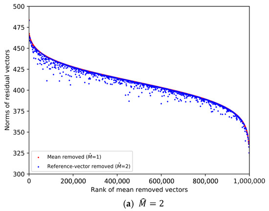
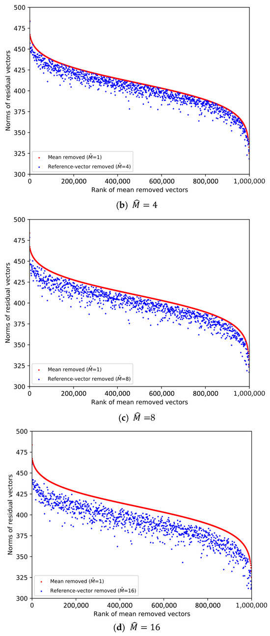
Figure 1.
Comparison of the norms of residual vectors for part of the SIFT1M dataset. The rank is based on the norms of the residual vectors when , which is used as a baseline. The red dots represent the norms of selected samples after subtracting their mean, sorted in descending order by norm. The blue dots represent the magnitudes of the same samples after removing the learned reference-vector.
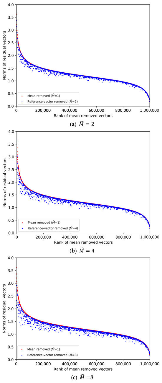
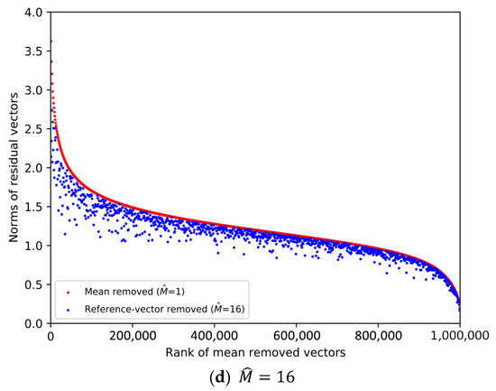
Figure 2.
Comparison of the norms of residual vectors for part of the GIST1M dataset. The rank is based on the norms of the residual vectors when , which is used as a baseline. The red dots represent the norms of selected samples after subtracting their mean, sorted in descending order by norm. The blue dots represent the magnitudes of the same samples after removing the learned reference-vector.
In Figure 1 and Figure 2, the increasingly larger gap between the blue dots and red dots demonstrates the better result of reducing the norms of the residual vectors. To illustrate the trend clearly, only 1000 database vectors are plotted. We rank the norms of the mean-removed vectors () in descending order and set the condition as a baseline, which is shown by the red dots. The blue dot and red dot with the same x-axis value represent two residual vectors of the same database vector. We can see that the larger is, the lower the overall distribution of the blue dots is. Therefore, it is more efficient to remove redundancy as the dimension of the reference-vector becomes larger.
However, it is worth noting that we also need to quantize the reference-vectors and store the VQ codeword indices. As the value of becomes larger, it is increasingly difficult to quantize the reference-vector, that is, the quality of the quantized reference-vectors drops.
Therefore, the value of needs to be considered as a trade-off between the effectiveness of removing redundancy and the quality of the quantized reference-vectors. Table 1 shows the overall quantization distortion for different in different datasets when , which is a typical set of parameters. Considering the dimension of the dataset vectors, we set as the integer power of 2 so that the dimension D can be equally divided for each subspace.

Table 1.
Quantization distortion for different
in different datasets ().
In this paper, we determine the optimal for different datasets through experiments.
3.4. Codebook Learning
In RvRPQ, to control the complexity of the algorithm, we set the dimension of the reference-vectors as a relatively small value, on which we perform vector quantization. In addition, product quantization is implemented for high-dimensional residual vectors. Therefore, we need to learn two codebooks in total, which are the VQ codebook for the reference-vectors and the PQ codebook for the residual vectors. The size of the VQ codebook is . For product quantization, we decompose the space into sub-spaces and allocate centroids for each subspace. Therefore, the PQ codebook has sub-codebooks for sub-spaces, and the size of each sub-codebook is .
In this paper, we use non-independent quantization for the VQ quantizer and PQ quantizer. It means that the dataset vectors subtract the quantized reference-vectors rather than the exact reference-vectors.
To further elaborate the non-independent quantizer, we start with the VQ quantizer for reference-vectors. The VQ codebook is obtained by quantizing the reference-vectors in the learning set. And represents the quantized reference-vector
We expand the dimension of instead of the exact . And the residual vector is defined as
where is the -th component of . And the dimension of is . Then, we implement LBG on sub-vectors of separately to train the PQ codebook . The effect of decorrelation is related to the quality of . Therefore, both and play an important role in our method. The detailed process of the codebook learning is shown in Figure 3.
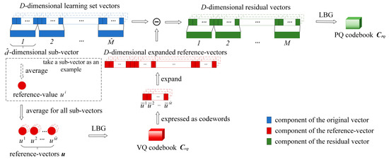
Figure 3.
The process of learning VQ codebook
and PQ codebook .
3.5. Encoding and Searching Process
Firstly, in the encoding process, is defined as the reference-vector for the database vector , and the subscript is added to distinguish between the database vector and the query vector:
And we quantize with the VQ codebook to obtain its VQ codeword index. And the quantized reference-vector is expressed as
The code length of each VQ index is bits. In addition, the Euclidean distances between any two codewords are stored in the look-up table so that the online distance calculation is simplified as a look-up table operation, which speeds up the online searching process. Secondly, the PQ codeword indices are obtained by quantizing the residual vectors , which concatenate indices with the code length of ,
In the ANN searching process, is defined as the reference-vector of the query vector , which is quantized to a VQ codeword. The distances between and the reference-vectors of database vectors are approximated by the symmetric distances. The reason why we use the symmetric distances is that only a look-up table is needed to obtain the distances between the codewords, which have been calculated and stored offline. Therefore, the method has almost little impact on the search speed. We further calculate the Euclidean distances between each sub-vector of the residual vector and every sub-codeword in the corresponding subspace. The distances are stored in the look-up table , which is calculated online for different query vectors (Algorithm 1).
| Algorithm 1 Encoding the database vectors |
| Input: The D-dimensional database set ; VQ codebook for reference-vectors ; PQ codebook for residual vectors . |
| Output: Indices for reference-vectors and for residual vectors ; 1.Load the dimension of codewords in ; 2. for do 3.Decompose into sub-vectors ; 4.Average the sub-vectors, respectively, to obtain reference-vector ; 5.Quantize u with to obtain the index and the quantized reference-vector 6.Expand with , the dimension of I is , and calculate the residual vector 7.Quantize with to obtain the PQ index ; 8.Return and . 9. end for |
The searching distance is determined by both the distance between and and the distance between and . We assume that the quantized reference-vector after expanding is written as
where the dimension of is .
According to the definition of the reference-vector and residual vector, the total distance between the query and the database vector is given as
It can be expressed as the squared distance
It goes to
The high-dimensional residual vector is included in the calculation of the inner product term. To obtain the exact inner product value, a huge amount of online calculation is required, which brings unbearable additional complexity. Therefore, we ignore the inner product term. And according to the recall rate of our experiment in Section 4, the inner product term has almost no impact on the final search accuracy. Then, the squared distance can be approximated as
The distance between the residual vectors is approximated by the asymmetric distance. And the distance between the reference-vectors is approximated by the symmetric distance. Thus, we rewrite it as
The squared distance can be computed efficiently using the look-up tables and . Then, we assign R as the length of the candidate list. If the nearest neighbor is ranked in the top R positions, it is regarded as a correct and successful search (Algorithm 2).
| Algorithm 2 Process of ANN search |
| Input: The D-dimensional query vector ; VQ codebook for reference-vectors ; PQ codebook for residual vectors ; indices and for database vectors; look-up table . |
| Output: Top R nearest neighbors of in database. 1.Load the dimension of codewords in ; 2.Decompose into sub-vectors; 3.Average the sub-vectors, respectively, to obtain reference-vector ; 4.Expand the quantized reference-vector as Algorithm 1; 5.Read the distances from look-up table for every database vectors ; 6.Calculate the residual vector:; 7.Calculate the distances between and each PQ codeword and store them in look-up table ; 8.Read the distances from look-up table for every database vectors ; 9.Rank the database vectors in ascending order in terms of ; 10.Return R nearest neighbors of . |
4. Experiments
In this section, we first introduce the setup of the experiments. Then, the performance of our proposed method (RvRPQ) is evaluated through comparative experiments with mean-removed product quantization (MRPQ) and product quantization (PQ) for the exhaustive search. Finally, we analyze the time complexity and memory cost of RvRPQ.
4.1. Setup
Two datasets are used in the experiment: SIFT1M [32] and GIST1M [33]. Both of the datasets consist of learning set, database set and query set. Table 2 summarizes the specific information of the datasets.
Table 2.
Summary of the SIFT1M and GIST1M datasets.
These datasets are publicly available on http://corpus-texmex.irisa.fr/ (accessed on 1 July 2010).
Prior to inputting the query vectors, several offline preprocessing steps were conducted. These include pre-training the vector quantization codebook for the reference-vectors and the product quantization codebooks for the residual vectors. Additionally, the symmetric distances between codewords were calculated and stored in a look-up table . This precomputed distance look-up table facilitates efficient retrieval during the query phase by reducing the need for real-time computation.
To verify the enhancement of the ANN search accuracy after removing the reference-vector, we assign the parameter of RvRPQ as respectively. When , the method RvRPQ degenerates to MRPQ.
The size of the reference-vector codebook is set as , that is, 8 bits are allocated to store a codeword index of the reference-vector.
For the product quantization of the residual vectors, we assign the number of sub-spaces as . The size of each sub-codebook is . Thus, the code lengths of the residual vectors are bits, bits and bits, respectively.
The recall rate is an indicator to measure the ANN search accuracy, which is expressed as recall@R. For a single query , if the groundtruth falls in top R ranked positions, we assume the search to be successful and record the correct search result as 1; otherwise, it is recorded as 0. The search results of all queries in the query set are summed up and then divided by the number of queries.
The above result is referred to as recall@R when the maximal successful ranked position of the groundtruth is R.
All experiments were conducted on a desktop computer equipped with an Intel i7-8700 CPU @ 3.20 GHz and 32 GB of RAM.
4.2. Experimental Results
The experimental results are shown in Figure 4, Figure 5, Figure 6 and Figure 7, the x-axis shows the R value in recall@R, representing the number of top-ranked results retrieved for each query. The y-axis shows the recall@R, defined as the fraction of true nearest neighbors successfully retrieved within the top R results. Higher curves indicate better retrieval accuracy. Results are averaged over all queries in the datasets.
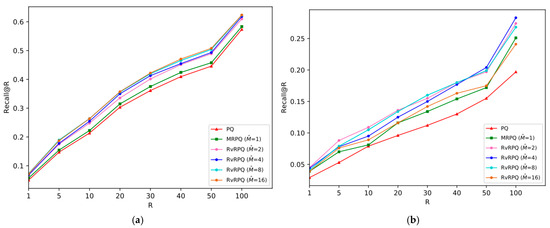
Figure 4.
Comparisons of PQ (the code length
bits), MRPQ ( bits) and RvRPQ ( bits) with different on two datasets, where and . (a) SIFT1M; (b) GIST1M.
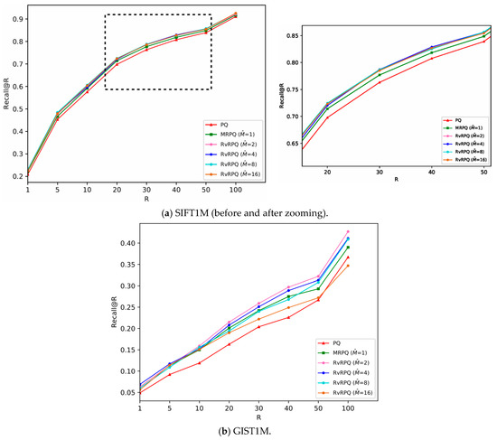
Figure 5.
Comparisons of PQ (the code length
bits), MRPQ ( bits) and RvRPQ ( bits) with different on two datasets, where and . (a) SIFT1M; (b) GIST1M.
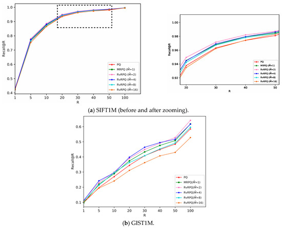
Figure 6.
Comparisons of PQ (the code length
bits), MRPQ ( bits) and RvRPQ ( bits) with different on two datasets, where and . (a) SIFT1M; (b) GIST1M.
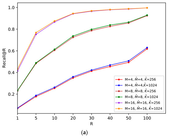
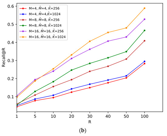
Figure 7.
Comparisons of the size of
on two datasets, where and . (a) SIFT1M; (b) GIST1M.
For SIFT1M: Figure 4a, Figure 5a and Figure 6a demonstrate the recall rate of RvRPQ when the number of PQ sub-spaces ,8,16, respectively. When , the search accuracy recall@R of RvRPQ with is significantly improved compared to MRPQ and PQ. Among them, the performance of is the best. The recall@100 of PQ, MRPQ and RvRPQ () is 57.36%, 58.34% and 62.35%, respectively. The search accuracy of RvRPQ is about 4% higher than MRPQ and 5% higher than PQ. When , the search accuracy of the three methods is relatively close. We can observe the zoom view on the right side of Figure 5a and Figure 6a. They illustrate that the highest curve always belongs to RvRPQ. In addition, we can figure out the optimal for various setups according to the experiments. For instance, assigning as 2 brings the best performance for SIFT1M when . As for , can be flexibly set as 2, 4, 8, 16.
For GIST1M: Figure 4b, Figure 5b and Figure 6b illustrate the recall rate when the number of sub-spaces of PQ ,8,16, respectively. Regardless of the value for , it is always a satisfying choice for or for GIST1M dataset. For example, when , the recall@100 of PQ, MRPQ and RvRPQ () is 19.70%, 25.10% and 28.30%. The search accuracy of RvRPQ increases by 8.60% compared to PQ and 3.20% compared to MRPQ. When the recall@100 of PQ, MRPQ and RvRPQ () is 36.70%, 39.00% and 41.10%. It rises by 4.40% compared to PQ, and 2.10% compared to MRPQ.
In terms of the analysis of the reference-vector in Section 3, when increases, the norms of the residual vectors reduce more, that is, the effectiveness of decorrelation is better. But when increases, it is more difficult for the quantization of the reference-vector, and the quantization distortion will significantly rise. Therefore, the parameter adjustment of is a compromise between the effect of redundancy removing and the accuracy of quantizing the reference-vector. According to the experiment, it can be seen that for the SIFT1M dataset, when is set as 8, the performance of RvRPQ is always better than MRPQ regardless of . Thus, is the best choice for SIFT1M. While for the GIST1M dataset, when is set as 4, the overall performance is the best.
In order to reduce the quantization distortion of the reference-vector, instead of using a smaller , we can consider increasing the number of centroids of vector quantization, which improves the final search accuracy at the expense of a certain memory cost. We compare the recall@R when and .
It can be noticed from Figure 7 that when increases, the recall@R on both datasets increases. Therefore, if there is requirement for high accuracy, we can meet the demand by enlarging the size of VQ codebook for the reference-vector.
4.3. Discussions
In this section, we compare the memory cost and time complexity of RvRPQ and MRPQ.
Memory cost: (1) For the ANN search, the main storage consumption is the codeword indices of the database vectors. MRPQ is a special case of our proposed RvRPQ in the case of . The index structure of them is exactly the same, which consists of two parts: the index of the reference-vector and the index of the residual vector. A total of ) bits need to be allocated for the whole indices. (2) Compared to MRPQ, the memory cost of RvRPQ is only increased by the VQ codebook for the reference-vectors. The dimension of the VQ codeword is in RvRPQ, while in MRPQ the dimension is 1. Thus, there are floating-point values in the VQ codebook for RvRPQ, while there are floating-point values for MRPQ. Because is much smaller than the size of the database , the increased storage consumption for the codebook is obviously negligible. Therefore, the memory cost is almost the overall same for RvRPQ and MRPQ.
Time complexity: When figuring out the reference-vector, it is necessary to carry out times of addition and times of division for each vector. The time complexity of division is higher than that of addition. Thus, while gets larger, the time complexity increases. But for high-dimensional vectors, the value of is much larger, so the rising of the time complexity for this part can be ignored. For the distance calculation of the preprocessing stage, MRPQ only has to calculate the scalar distance, while RvRPQ has to calculate the distance among -dimensional vectors. However, only look-up table operations are needed to obtain the distances. In addition, there is no difference in the time complexity of calculating the distance among the residual vectors. Thus, as shown in Table 3, as , this extra overhead is negligible in practice and the online time complexity of RvRPQ and MRPQ is almost the same.
Table 3.
Online time complexity of RvRPQ and MRPQ for each query.
The search time for different methods is also given in Table 4.
Table 4.
Search time for different methods.
The experimental results in Table 4 show that RvRPQ only incurs a slight increase in search time compared to MRPQ due to the additional cost of retrieving and applying the reference-vector for each data point. However, this increase is minimal, as the core distance computation via look-up tables remains unchanged and the majority of operations are still performed offline. In general, the memory cost and the online time complexity of RvRPQ and MRPQ are almost the same. In this case, the final ANN search accuracy has been significantly improved.
5. Conclusions
In this paper, we propose a decorrelation method for product quantization, which is called reference-vector removed product quantization (RvRPQ). In order to remove the redundancy in the database vector, we optimally extract a reference-vector and quantize it separately. Through mathematical derivation, we can determine the optimal reference value, which is the mean of the sub-vector. In addition, we determine the optimal dimension of the reference-vector by experiments. Compared to MRPQ, our proposed RvRPQ achieves a substantial improvement in Recall@R while maintaining identical memory cost and introducing negligible time complexity increase in different datasets.
Author Contributions
Conceptualization, Y.W. and X.W.; methodology, Y.W. and X.W.; Y.W. and C.X.; validation, Y.W. and C.X.; formal analysis, Y.W. and C.X.; investigation, Y.W. and X.W.; resources, Y.W. and X.W.; data curation, Y.W. and C.X.; writing—original draft preparation, Y.W. and C.X.; writing—review and editing, Y.W. and X.W.; supervision, Y.W. and X.W. All authors have read and agreed to the published version of the manuscript.
Funding
This research was funded by The Ph.D. Stand-up Fund of Xi’an University of Technology (Grant No. 108-451121002).
Institutional Review Board Statement
Not applicable.
Informed Consent Statement
Not applicable.
Data Availability Statement
The original contributions presented in this study are included in the article. Further inquiries can be directed to the corresponding author.
Conflicts of Interest
The authors declare no conflicts of interest. The funders had no role in the design of the study; in the collection, analyses, or interpretation of data; in the writing of the manuscript; or in the decision to publish the results.
Abbreviations
The following abbreviations are used in this manuscript:
| VQ | Vector quantization |
| PQ | Product quantization |
| ANN | Approximate nearest neighbor |
References
- Sarwar, B.; Karypis, G.; Konstan, J.; Riedl, J. Item-based collaborative filtering recommendation algorithms. In Proceedings of the 10th International Conference on World Wide Web, Hong Kong, China, 1–5 May 2001. [Google Scholar]
- Ning, Q.; Zhu, J.; Zhong, Z.; Hoi, S.C.; Chen, C. Scalable image retrieval by sparse product quantization. IEEE Trans. Multimed. 2017, 19, 586–597. [Google Scholar] [CrossRef]
- Nister, D.; Stewenius, H. Scalable recognition with a vocabulary tree. In Proceedings of the IEEE Conference on Computer Vision and Pattern Recognition, New York, NY, USA, 17–22 June 2006. [Google Scholar]
- Li, W.; Zhang, Y.; Sun, Y.; Wang, W.; Li, M.; Zhang, W.; Lin, X. Approximate nearest neighbor search on high dimensional data—Experiments, analyses, and improvement. IEEE Trans. Knowl. Data Eng. 2019, 32, 1475–1488. [Google Scholar] [CrossRef]
- Buzo, A.; Gray, A.H.; Member, S.; Gray, R.M.; Markel, J.D.; Member, S. Speech coding based upon vector quantization. IEEE Trans. Acoust. Speech Signal Process. 1980, 28, 562–574. [Google Scholar] [CrossRef]
- Muja, M.; Lowe, D.G. Scalable nearest neighbor algorithms for high dimensional data. IEEE Trans. Pattern Anal. Mach. Intell. 2014, 36, 2227–2240. [Google Scholar] [CrossRef] [PubMed]
- J’egou, H.; Douze, M.; Schmid, C. Product quantization for nearest neighbor search. IEEE Trans. Pattern Anal. Mach. Intell. 2018, 33, 117–128. [Google Scholar] [CrossRef] [PubMed]
- Jin, Z.; Li, C.; Lin, Y.; Cai, D. Density sensitive hashing. IEEE Trans. Cybern. 2014, 44, 1362–1371. [Google Scholar] [CrossRef] [PubMed]
- Heo, J.-P.; Lee, Y.; He, J.; Chang, S.-F.; Yoon, S.-E. Spherical hashing: Binary code embedding with hyperspheres. IEEE Trans. Pattern Anal. Mach. Intell. 2015, 37, 2304–2316. [Google Scholar] [CrossRef] [PubMed]
- Gan, J.; Feng, J.; Fang, Q.; Ng, W. Locality-sensitive hashing scheme based on dynamic collision counting. In Proceedings of the 2012 ACM SIG-OD International Conference on Management of Data, Scottsdale, AZ, USA, 20–24 May 2012. [Google Scholar]
- Harwood, B.; Drummond, T. Fanng: Fast approximate nearest neighbourgraphs. In Proceedings of the IEEE Conference on Computer Vision and Pattern Recognition, Las Vegas, NV, USA, 27–30 June 2016. [Google Scholar]
- Wang, J.; Wang, J.; Zeng, G.; Tu, Z.; Gan, R.; Li, S. Scalable k-NN graph construction for visual descriptors. In Proceedings of the IEEE Conference on Computer Vision and Pattern Recognition, Providence, RI, USA, 16–21 June 2012. [Google Scholar]
- Babenko, A.; Lempitsky, V. Tree quantization for large-scale similarity search and classification. In Proceedings of the IEEE Conference on Computer Vision and Pattern Recognition, Boston, MA, USA, 7–12 June 2015. [Google Scholar]
- Babenko, A.; Lempitsky, V. Additive quantization for extreme vector compression. In Proceedings of the IEEE Conference on Computer Vision and Pattern Recognition, Columbus, OH, USA, 23–28 June 2014. [Google Scholar]
- Wang, J.; Zhang, T. Composite quantization. IEEE Trans. Pattern Anal. Mach. Intell. 2018, 41, 1308–1322. [Google Scholar] [CrossRef] [PubMed]
- Zhang, T.; Qi, G.-J.; Tang, J.; Wang, J. Sparse composite quantization. In Proceedings of the IEEE Conference on Computer Vision and Pattern Recognition, Boston, MA, USA, 7–12 June 2015. [Google Scholar]
- Brandt, J. Transform coding for fast approximate nearest neighbor search in high dimensions. In Proceedings of the IEEE Conference on Computer Vision and Pattern Recognition, San Francisco, CA, USA, 13–18 June 2010. [Google Scholar]
- Heo, J.-P.; Lin, Z.; Yoon, S.-E. Distance encoded product quantization for approximate k-nearest neighbor search in high-dimensional space. IEEE Trans. Pattern Anal. Mach. Intell. 2018, 41, 2084–2097. [Google Scholar] [CrossRef] [PubMed]
- Fan, J.; Wang, Y.; Song, W.; Pan, Z. Flexible product quantization for fast approximate nearest neighbor search. Multimed. Tools Appl. 2024, 83, 53243–53261. [Google Scholar] [CrossRef]
- Martinez, J.; Clement, J.; Hoos, H.H.; Little, J.J. Revisiting additive quantization. In Proceedings of the European Conference on Computer Vision, Amsterdam, The Netherlands, 11–14 October 2016. [Google Scholar]
- Baranchuk, D.; Babenko, A.; Malkov, Y. Revisiting the inverted indices for billion-scale approximate nearest neighbors. In Proceedings of the European Conference on Computer Vision, Munich, Germany, 8–14 September 2018. [Google Scholar]
- Babenko, A.; Lempitsky, V. The inverted multi-index. IEEE Trans. Pattern Anal. Mach. Intell. 2015, 37, 1247–1260. [Google Scholar] [CrossRef]
- Ge, T.; He, K.; Ke, Q.; Sun, J. Optimized product quantization. IEEE Trans. Pattern Anal. Mach. Intell. 2014, 36, 744–755. [Google Scholar] [CrossRef]
- Wang, Y.; Pan, Z.; Li, R. A new cell-level search based non-exhaustive approximate nearest neighbor (ann) search algorithm in the framework of product quantization. IEEE Access 2019, 7, 37059–37070. [Google Scholar] [CrossRef]
- Pan, Z.; Wang, L.; Wang, Y.; Liu, Y. Product quantization with dual-codebooks for approximate nearest neighbor search. Neurocomputing 2020, 401, 59–68. [Google Scholar] [CrossRef]
- Song, W.; Wang, Y.; Pan, Z. A novel cell partition method by introducing Silhouette Coefficient for fast approximate nearest neighbor search. Inf. Sci. 2023, 642, 119216. [Google Scholar] [CrossRef]
- Wu, X.; Guo, R.; Suresh, A.T.; Kumar, S.; Holtmann-Rice, D.N.; Simcha, D.; Yu, F. Multiscale quantization for fast similarity search. In Advances in Neural Information Processing Systems; Neural Information Processing Systems: Red Hook, NY, USA, 2017. [Google Scholar]
- Yang, J.; Chen, B.; Xia, S.-T. Mean-removed product quantization for large-scale image retrieval. Neurocomputing 2020, 406, 77–88. [Google Scholar] [CrossRef]
- Gersho, A.; Gray, R.M. Vector Quantization and Signal Compression; Springer Science & Business Media: New York, NY, USA, 2012. [Google Scholar]
- Wu, Z.; Yu, J. Vector quantization: A review. Front. Inf. Technol. Electron. Eng. 2019, 20, 507–524. [Google Scholar] [CrossRef]
- Matsui, Y.; Uchida, Y.; J’egou, H.; Satoh, S. A survey of product quantization. ITE Trans. Media Technol. Appl. 2018, 6, 2–10. [Google Scholar] [CrossRef]
- Lowe, D.G. Distinctive image features from scale-invariant keypoints. Int. J. Comput. Vis. 2004, 60, 91–110. [Google Scholar] [CrossRef]
- Oliva, A.; Torralba, A. Modeling the shape of the scene: A holistic representation of the spatial envelope. Int. J. Comput. Vis. 2001, 42, 145–175. [Google Scholar] [CrossRef]
Disclaimer/Publisher’s Note: The statements, opinions and data contained in all publications are solely those of the individual author(s) and contributor(s) and not of MDPI and/or the editor(s). MDPI and/or the editor(s) disclaim responsibility for any injury to people or property resulting from any ideas, methods, instructions or products referred to in the content. |
© 2025 by the authors. Licensee MDPI, Basel, Switzerland. This article is an open access article distributed under the terms and conditions of the Creative Commons Attribution (CC BY) license (https://creativecommons.org/licenses/by/4.0/).