Article

Benchmarking ML Approaches for Earthquake-Induced Soil Liquefaction Classification

1
Department of Mechanical Engineering, Faculty of Engineering, Istanbul University-Cerrahpasa, 34320 Istanbul, Turkey
2
Department of Mechanical Engineering, Faculty of Engineering & Architecture, Recep Tayyip Erdogan University, 53100 Rize, Turkey
3
Department of Mining and Mineral Extraction, Balikesir Vocational School, Balikesir University, 10185 Balikesir, Turkey
4
Department of Geological Engineering, Faculty of Engineering, Balikesir University, 10185 Balikesir, Turkey
*
Author to whom correspondence should be addressed.
Appl. Sci. 2025, 15(21), 11512; https://doi.org/10.3390/app152111512
Submission received: 9 October 2025 / Revised: 20 October 2025 / Accepted: 25 October 2025 / Published: 28 October 2025
(This article belongs to the Special Issue Soil Liquefaction in Geotechnical Engineering)

Abstract

Earthquake-induced soil liquefaction represents a critical geotechnical challenge due to its nonlinear soil–seismic interactions and its impact on structural safety. Traditional empirical methods often rely on simplified assumptions, limiting their predictive capability. This study develops and compares six machine learning (ML) classifiers—namely, Support Vector Machine (SVM), Artificial Neural Network (ANN), k-Nearest Neighbor (kNN), Random Forest (RF), Decision Tree (DT), and Naïve Bayes (NB)—to evaluate liquefaction susceptibility using an original dataset of 461 soil layers obtained from borehole penetration tests in the Edremit region (Balıkesir, NW Turkey). The models were trained and validated using normalized geotechnical and seismic parameters, and their performance was assessed based on accuracy, precision, recall, F1 score, and area under the receiver operating characteristic curve (AUC). Results demonstrate that SVM, ANN, and kNN consistently outperformed other models, achieving test accuracies above 93%, F1 scores exceeding 98%, and AUC values between 0.933 and 0.953. In contrast, DT and NB exhibited limited generalization (test accuracy of 84–88% and AUC of 0.78–0.82), while RF showed partial overfitting. In contrast, DT and NB exhibited weaker generalization, with test accuracies of 84% and 88% and AUC values of 0.78 and 0.82, respectively, while RF indicated partial overfitting. The findings confirm the superior capability of advanced ML models, particularly SVM, ANN, and kNN, in capturing complex nonlinear patterns in soil liquefaction. This study provides a robust framework and original dataset that enhance predictive reliability for seismic hazard assessment in earthquake-prone regions.

1. Introduction

Earthquakes are among the most destructive natural events, often resulting in significant loss of life and severe economic damage. The extent of these losses depends on several factors, including the dynamic properties of the building, ground–building interaction, and the behavior of the ground. The most critical ground deformations induced by earthquakes include surface faulting, soil amplification, and soil liquefaction.
Soil liquefaction induced by earthquakes occurs due to the propensity of loose, saturated soils to contract in volume when subjected to shear stresses such as cyclic or shock loading. Under such stress conditions, the volume of the void decreases, while the pressure of the pore water increases due to the impermeability of the soils, which hinders the release of water. Consequently, this sudden rise in pore water pressure leads to reductions in effective stress, shear strength, and soil density. When the shear strength of the soil becomes lower than the static shear stress, significant deformations occur, rendering the soil in a liquefied state [1]. Coarse-grained soils such as sand, silty sand, non-plastic silt, and gravel are particularly susceptible to liquefaction during earthquakes, especially when underlain or interlayered with low-permeability materials. The primary factors influencing soil liquefaction include the depth of the groundwater table, the index properties of the soil, the physical structure of soil particles, soil permeability, relative density, the age of the deposit, evidence of paleo-liquefaction, and the magnitude of external loading and environmental conditions [2]. Liquefaction may lead to a significant reduction in bearing capacity, excessive settlement, and horizontal displacement. Typical surface manifestations of this phenomenon include sand boils and lateral spreading of surficial soils. According to Dengiz [3], such events are particularly common in areas underlain by alluvial soils. This is because these soils are formed by river-borne sediments and are characterized by sudden changes in the vertical and horizontal distribution of particles over relatively short distances.
Although the impacts of liquefaction on engineering structures have long been known, engineers began studying the subject after the 1964 earthquakes in Alaska [4] and Niigata [5]. The 1989 Loma Prieta earthquake [6], the 1995 Great Hanshin earthquake [7], the 1999 Chi-Chi earthquake [8], the 1999 Kocaeli-Adapazari earthquake [9], the 2010 Canterbury earthquake [10], the 2018 Central Sulawesi earthquake [11], and the 2023 Kahramanmaraş earthquake [12] are major events where liquefaction played a significant role in the damage of settlement areas.
The liquefaction potential of soil may be assessed using a variety of procedures [13]. The empirical method based on field observations from several earthquake occurrences was the first method for determining ground liquefaction potential [14]. This strategy later resulted in the creation of semi-theoretical derivations. Some semi-theoretical methodologies employ common field-testing procedures such as standard penetration testing (SPT) [15,16,17,18], shear wave velocity ( V S ) testing [19,20,21,22,23], and cone penetration testing [24,25,26]. However, these approaches are not always exact because they are based on a small number of “limit cases” acquired from field observations [27,28,29]. Although there are many classic forecasting methodologies, such as statistical and laboratory testing methods, they all have drawbacks. For instance, laboratory test predictions are frequently incorrect because they rely on samples and testing processes [30]. The classic statistical approach is also insufficiently precise to suit practical engineering requirements [31]. Furthermore, the complexity of the elements that influence soil liquefaction, the highly nonlinear correlations between parameters and liquefaction results, the uncertainty of ground parameters, and the randomness of seismic events make it difficult to pick effective empirical equations [32]. With the development of soft computing techniques, many scholars have focused on developing machine learning (ML) models for prediction of ground liquefaction potential. An important feature of ML models is their ability to create accurate predictions based solely on the obtained data. This reduces the need for explicit knowledge of the underlying relationships between input and output variables. In addition, ML models can help uncover both linear and nonlinear relationships between these variables [33,34]. This research aims to explore the fuzzy space between various proposed transition zones that separate liquefiable regions from non-liquefiable regions. Table 1 provides an overview of previous studies that employed ML models to predict soil liquefaction, detailing the classification algorithms, datasets, and input parameters employed in these studies.
This study employed empirical data obtained from borehole investigations and laboratory evaluations to classify soil liquefaction in the Edremit residential area (Balıkesir, NW Turkey) [13]. The Edremit settlement lies along the Edremit Fault Zone, an extension of the North Anatolian Fault Zone, and is particularly characterized by liquid alluvium. Historically, the region has experienced destructive seismic activity, including a magnitude 6.8 earthquake in 1944. Although numerous ML-based studies have been conducted for liquefaction prediction, most have relied on international or region-specific datasets and have seldom incorporated borehole data from northwestern Turkey. This gap has limited both the generalizability and the regional relevance of existing predictive models.
To address this shortcoming, six ML models—specifically, k-Nearest Neighbor (kNN) [57,58], Artificial Neural Network (ANN) [59], Decision Tree (DT) [60], Random Forest (RF) [29], Support Vector Machine (SVM) [35], and Naive Bayes (NB) [28,61]—were utilized to forecast soil liquefaction induced by earthquakes. The kNN technique operates by evaluating the proximity of data points in feature space to derive labels, rendering it applicable to both classification and regression tasks. ANN mimics human brain structure and function, making exact predictions by processing incoming data through interconnected neuron layers. The DT method simplifies decision-making processes by iteratively partitioning the feature space. Similarly, RF constructs multiple decision trees and consolidates their predictions to enhance adaptability and generalization. SVM specializes in binary and multi-class classification by identifying the optimal hyperplane in feature space for maximal class separation. Despite their simplicity, NB classifiers offer effective probabilistic classification by assuming feature independence, making them particularly suited for tasks such as text classification and the handling of high-dimensional data challenges. The performance of the prediction models used in this study was evaluated according to accuracy, precision, recall, F1 score, and true-positive and false-positive rates.
The main contributions of this work include (i) finding the best classification ML model for earthquake-induced soil liquefaction; (ii) providing an original dataset from the Edremit region in Balikesir, NW Turkey, which has never been used for ML; and (iii) offering insights into each ML model with respect to its practical implications for soil liquefaction prediction. The remainder of this paper is organized as follows: Section 2 explains the material and methods, including data collection and the details of the ML models used in the study. Section 3 presents the experimental results and a performance comparison of the ML models. Finally, Section 4 presents the conclusions.

2. Material and Methods

2.1. Description of the Study Area

The Edremit district of Balikesir Province (Turkey), the study area as shown in Figure 1, is situated on the southern coast of the Edremit Gulf, part of the Aegean Sea. The research area, Edremit village, is situated on the southern branch of the North Anatolian Fault (NAF). The NAF is recognized as one of the most seismically active regions in the world (See Figure 1). The westward movement of Anatolia in relation to Eurasia since the Pliocene is attributed to the NAF, which forms the border between the Eurasian and Anatolian plates [62,63].
According to [63], the 1999 İzmit (Mw = 7.4) and Düzce (Mw = 7.2) earthquakes ruptured segments of the North Anatolian Fault (NAF). The southern branch of the NAF is characterized by several parallel and subparallel dextral strike–slip faults extending across the southern Marmara region [65]. North and west of the study area, major active faults include the Edremit Fault Zone (EFZ)—comprising the Zeytinli and Altınoluk segments—as well as the Evciler, Bekciler, Yenice–Gönen, Sarıköy, Çan, and Pazarköy faults (see Figure 1). Along the western termination of the southern branch, encompassing the EFZ and its surroundings, historical records indicate 30 earthquakes at 18 sites between 160 and 1898 AD [63,65]. During the instrumental period, the same branch produced several significant earthquakes, including the 1919 Ayvalık–Sarımsaklı (Mw = 7.2) [66], the 1944 Edremit (Mw = 6.4), and the 1953 Yenice (Mw = 7.2) events [65].
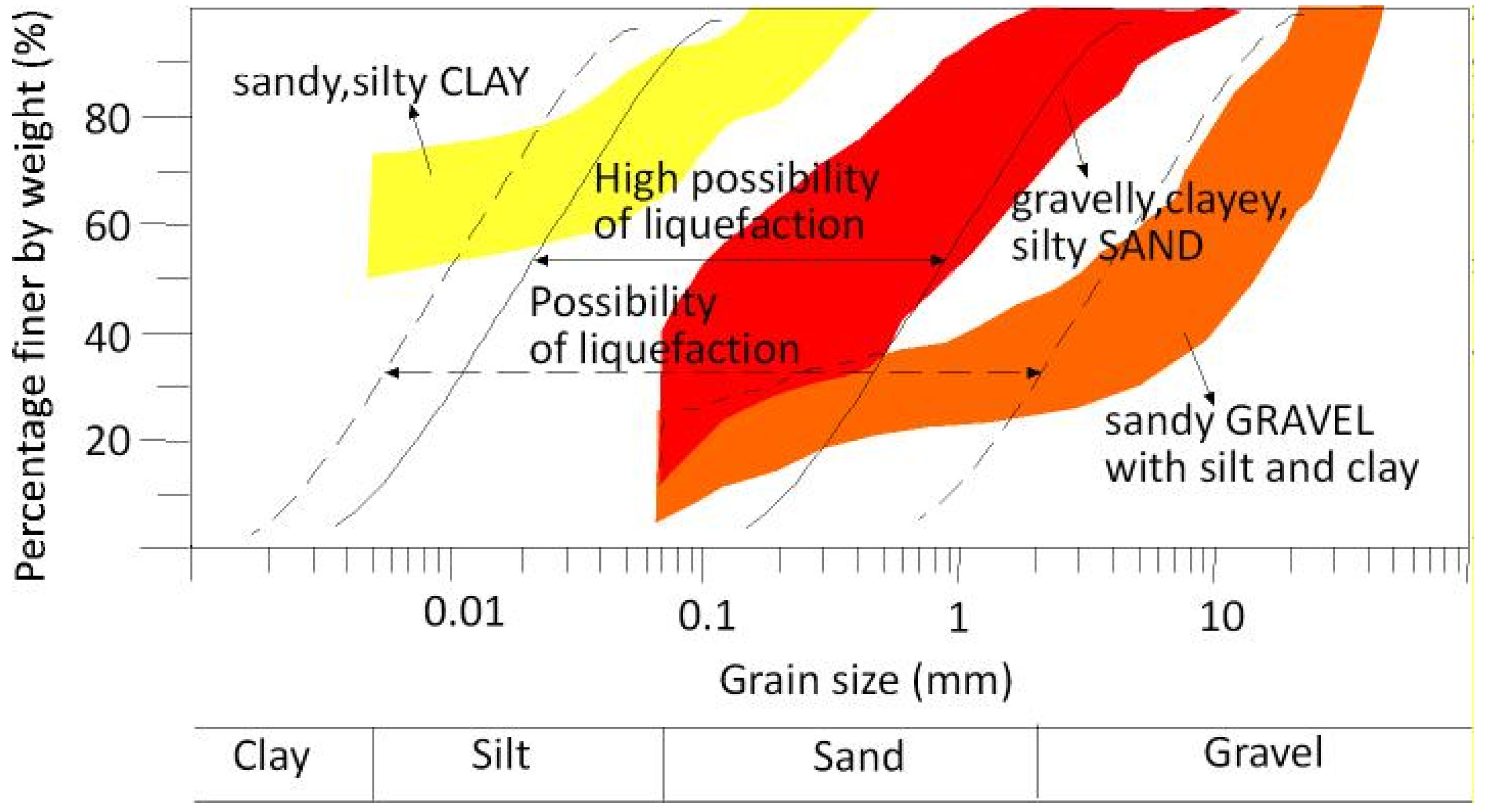
Sieve analysis reveals that the soil layers of the alluvial land were composed of three different soil textures: sandy, silty clay; gravelly, clayey, silty sand; and sandy gravel with clay and silt, as shown in Figure 2 [64]. In this study, liquefaction analyses were performed in the gravel, clay, and silty sand unit. The groundwater depth is <1.5 m in 62% of the study area, between 1.5–3.0 m in 28%, between 3.0–4.5 m in 6%, and >4.5 m in 4%.

2.2. Dataset

This research employed data obtained from standard penetration tests, as well as laboratory evaluations conducted on alluvial deposits situated in Edremit (Balıkesir, NW Turkey). Furthermore, the Turkey Active Fault Map and the Turkey Earthquake Hazard Map were utilized to ascertain the maximum ground acceleration value. Initially, the safety factor (FS) against liquefaction within the soil strata of these alluvial deposits was evaluated using a simplistic approach predicated on the SPT-N value [24]. The FS was derived as the cyclic resistance ratio (CRR) divided by the cyclic stress ratio (CSR). The CSR denotes the cyclic loading imposed on the soil as a result of seismic activity, whereas the CRR indicates the capacity of the soil to resist the onset of liquefaction. To accurately determine the FS, it is imperative to first comprehend the type of ground present. For FS > 1 , the classification of “liquefaction absent” was assigned, whereas FS 1 was categorized as “liquefaction present” [68,69]. The calculation of the CSR requires values for the maximum horizontal ground surface acceleration ( a m a x ), vertical total stress, and vertical effective stress. In order to compute the vertical total stress and vertical effective stress, it is essential to determine the depth of the underground water table, the thickness of the soil layer, and the unit weight of the soil.
The CRR value was determined using the SPT-N value, adjusted for the fine grain content ( ( N 1 ) 60 C S ). To achieve this, the SPT-N value ( N 30 ) was initially modified for the roller length, hammer energy, type of sampler, borehole diameter, and overburden stress [24]. Subsequently, the SPT-N value ( ( N 1 ) 60 ), which was corrected based on the aforementioned factors, was further adjusted for the fine grain proportion. Determining the FS value involves identifying a multitude of inputs, many of which may exhibit complex, non-linear interactions that require careful consideration to accurately model soil liquefaction. In this research, a m a x , z, SPT-N, and FC served as inputs in the prediction models for assessment of soil liquefaction classification. Upon establishing the occurrence or absence of liquefaction based on the FS of the analyzed soil layers, the prediction models were trained, and the ML models were subsequently evaluated based on the derived parameter values. Out of a total of 461 soil layers, 322 were allocated for training and 139 for testing. Furthermore, 313 liquefaction cases and 148 non-liquefaction cases were included in the dataset. The split was preserved in the train–test partition, with 233 liquefaction and 89 non-liquefaction cases in the training set and 80 liquefaction and 59 non-liquefaction cases in the test set. Outlier detection was performed by employing visual inspection of the box plots, and the dataset does not exhibit significant outlier behavior.

2.3. Model Development

The primary objective of this study is to develop a robust ML model capable of accurately predicting earthquake-induced soil liquefaction. To ensure the reliability and generalizability of the model, the dataset was randomly partitioned: 70% for training and 30% for testing. Prior to model training, it was essential to eliminate potential biases arising from the differing scales of geotechnical and seismic input variables. Let the input feature vector for each sample be expressed as follows:
x = x i , j
where i represents the input variable (i.e., a m a x , z, SPT-N, and FC) and j denotes the index of the sample.
Accordingly, the Z-score normalization technique was applied to remove the dimensional influence of inputs on the prediction process [70,71,72]. During normalization, the mean ( μ train , i ) and standard deviation ( σ train , i ) of each input variable were computed exclusively from the training dataset as follows:
μ train , i = 1 N train j = 1 N train x i , j
σ train , i = 1 N train 1 j = 1 N train ( x i , j μ train , i ) 2
where x i , j denotes the value of the ith input variable in the jth training sample and N train is the number of samples in the training set. Each feature in the training dataset was then normalized according to the standard Z-score formulation:
x i , j = x i , j μ train , i σ train , i
Subsequently, the same scaling parameters ( μ train , i and σ train , i ) obtained from the training data were used to normalize the test dataset as follows:
x i , k ( test ) = x i , k ( test ) μ train , i σ train , i
where x i , k ( test ) denotes the ith feature value of the kth sample in the test dataset. By refraining from recalculating normalization parameters for the validation and test datasets, this approach ensures complete data independence and prevents any potential information leakage that could bias the evaluation of model performance.
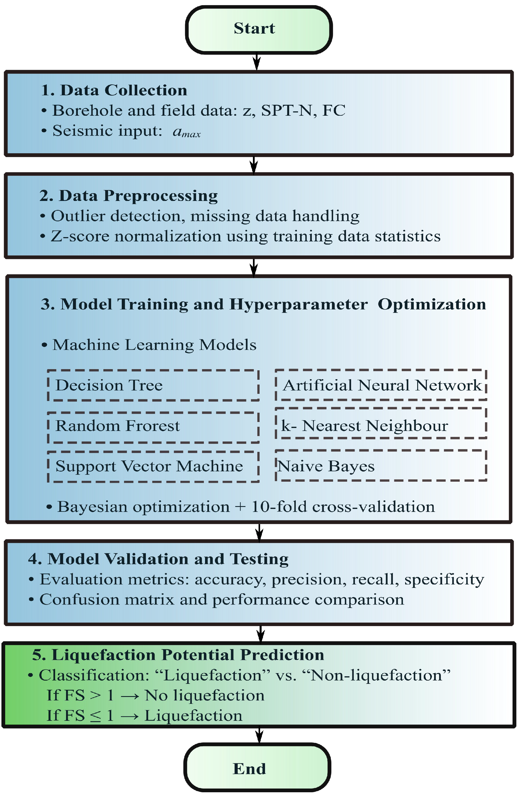
In addition, hyperparameter optimization plays a vital role in fine-tuning machine learning models and improving their performance on unseen data. Bayesian optimization is especially effective because it can explore the hyperparameter space efficiently with relatively few evaluations, manage noisy objective functions, and adapt to a wide range of optimization problems. This makes it a practical and reliable choice for maximizing model accuracy while keeping computational demands reasonable [73,74]. In this study, Bayesian optimization was used to systematically tune the hyperparameters of each model. For every ML model, the hyperparameter search was conducted within predefined parameter bounds appropriate to its architecture. The objective function was to minimize the classification error evaluated via 10-fold cross-validation on the training dataset. In each iteration, the validation accuracy from the held-out fold was used to update the candidate configuration and guide subsequent hyperparameter selection. Once convergence was achieved, the configuration producing the highest validation performance was adopted as the optimal set of hyperparameters. The general workflow of the proposed methodology is presented in Figure 3.
Six different classification algorithms were employed to represent a broad spectrum of machine learning approaches, including instance-based (kNN), margin-based (SVM), tree-based (DT, RF), probabilistic (NB), and connectionist (ANN) methods. The selected algorithms represent the main paradigms of supervised classification ML models, each offering distinct learning strategies and levels of interpretability. NB was included as a simple probabilistic baseline to illustrate how the assumption of feature independence affects predictive accuracy. DT and RF were chosen to compare a single-tree structure with its ensemble extension, as RF provides a more robust and stable learning mechanism widely adopted in data analysis. Overall, these six algorithms collectively cover the fundamental principles of supervised learning, enabling a comprehensive and balanced evaluation of model performance in predicting soil liquefaction potential.

2.3.1. k-Nearest Neighbor (kNN)

The k-Nearest Neighbor (kNN) algorithm, a non-parametric approach, is employed for both classification and regression tasks [57,75]. Its core principle revolves around assessing the similarity between data points. In classification, kNN predicts the class of a given data point by identifying its k nearest neighbors in the feature space and selecting the majority class among them. For regression tasks, it predicts the value of a target variable by averaging the values of the k nearest neighbors.
The fundamental concept in kNN is the notion of distance, which quantifies the similarity between two data points. The selection of a distance metric is contingent upon the characteristics of the data. The conventional distance metrics utilized in kNN are Euclidean distance, Manhattan distance, and Hamming distance [76]. Once the distance metric is defined, the kNN algorithm finds the set of k nearest neighbors of a given query data point x q from the training dataset, expressed as:
N k ( x q ) = argmin k d ( x q , x i )
where d ( · ) represents the chosen distance metric. The value of k is a hyperparameter that needs to be tuned for optimal performance on a specific dataset and task [77].
In classification problems, the class label of the query point x q is then determined based on the class labels of its neighbors in N k ( x q ) . A simple and commonly used approach is to assign the majority class label among the k nearest neighbors, formulated as:
y ^ q = argmax y x i N k ( x q ) δ ( y i , y )
where y ^ q is the predicted class label for x q , y i is the class label of the i th nearest neighbor, y denotes a class under consideration, and δ is the Kronecker delta function that returns 1 if y i = y and 0 otherwise.

2.3.2. Artificial Neural Network (ANN)

Artificial Neural Networks (ANNs) represent a class of computational models inspired by the structure and function of the human brain, designed to tackle complex learning tasks, including classification problems. ANNs process input data through a series of weighted connections and activation functions [78,79]. In the context of classification, ANNs are configured with an input layer representing features, hidden layers for information processing, and an output layer for class predictions [80,81]. The mathematical foundation of ANNs for classification encompasses several pivotal components crucial for their functioning. Firstly, within the hidden and output layers, each neuron calculates a weighted sum of its inputs, computed as the dot product of input values and corresponding weights acquired during network training. Following this computation, an activation function is applied to introduce non-linearity, which is essential for capturing complex data relationships. Notable activation functions include the sigmoid, tanh, and rectified linear unit (ReLU) functions, each influencing the capacity of the network to model intricate data patterns.
During the forward propagation phase, input data traverse through the network, with neuron activations computed. The determination of network performance hinges on the utilization of loss functions, such as cross-entropy and softmax loss, which measure the disparity between predicted and actual outputs. Moreover, the iterative refinement of network parameters occurs through backpropagation, a sophisticated algorithm designed to minimize the loss function by computing gradients with respect to the weights and adjusting them accordingly using gradient descent techniques. This iterative training process continues until the performance of the network converges to a satisfactory level, underscoring the meticulous approach employed in ANNs for achieving optimal classification outcomes.

2.3.3. Decision Tree (DT)

The Decision Tree (DT) method is a popular ML model used for classification tasks [75,82]. It constructs a tree-like structure where internal nodes represent feature tests, branches represent the outcomes of these tests, and leaf nodes represent the class labels. At the core of its functionality lies the selection of optimal feature tests and corresponding thresholds to split the data, guided by criteria such as Gini impurity or entropy to ensure maximal homogeneity within resulting subsets. The entropy value (E) and the Gini index (G) are calculated in Equations (8) and (9) [83].
E = i = 1 n p i log ( p i )
G = 1 i = 1 n p i 2
where n is the number of classes and p i is the probability of the ith condition. The feature test that minimizes entropy or Gini impurity is selected as the optimal splitting criterion for that node of the decision tree. This process is repeated recursively for each child node until a stopping criterion is met, such as reaching a maximum tree depth or a minimum number of samples per leaf. By iteratively partitioning the feature space based on the selected criteria, the decision tree constructs a hierarchical structure that efficiently assigns class labels to new instances.

2.3.4. Random Forest (RF)

The Random Forest (RF) method is a powerful ensemble learning algorithm used for classification tasks. It operates by constructing multiple decision trees during training and outputting the mode of the classes [44]. The mathematical background of the RF method for classification involves several key components, starting with the creation of multiple decision trees derived from bootstrapped samples of the original training data. Through this process, each decision tree is constructed by recursively partitioning the feature space, with randomness injected by considering only a subset of features at each node split. The number of features considered at each node is typically set as a hyperparameter and can greatly influence the performance of the RF model [84].
Once all trees are generated, their predictions are aggregated in the RF method using a majority voting scheme for classification tasks, leveraging the collective wisdom of individual trees to improve prediction accuracy. Additionally, the success of the RF method depends on carefully tuning its hyperparameters, such as the number of trees, maximum tree depth, and feature subset size. Techniques like cross-validation help optimize these parameters for maximum performance. The RF method is a powerful classification framework that combines multiple decision trees to produce robust and reliable predictions. It can also provide insights into feature importance by measuring each feature’s contribution to reducing impurity or increasing information gain across all trees.

2.3.5. Support Vector Machine (SVM)

The Support Vector Machine (SVM) method is predicated on identifying the optimal hyperplane that effectively separates different classes within the feature space. This hyperplane is strategically positioned to maximize the margin, defined as the distance between the hyperplane and the nearest data points from each class, referred to as support vectors [31]. By maximizing this margin, SVM strives to achieve optimal classification performance, thereby enhancing its ability to distinguish between different classes, even within complex, high-dimensional datasets. Additionally, SVM can manage nonlinearly separable data by mapping the original input space into a higher-dimensional feature space via a kernel function. The kernel function computes the dot product between data points in this higher-dimensional space without explicitly performing the transformation. Commonly used kernel functions include linear, polynomial, radial basis function, and sigmoid kernels. This methodological framework underpins the efficacy of SVM in various classification tasks, rendering it a popular choice in ML for its ability to address both linear and non-linear classification problems with high accuracy and robustness. Suppose that the empirical risk ( E R ) value is minimized as follows:
E R = 1 N i = 1 n | y i y ^ i |
where | y i y ^ i | is the ϵ -insensitive loss function, written as follows:
| y i y ^ i | = 0 , if | y i y ^ i |   < ε | y i y ^ i |     ε , otherwise
The proposed solution to this minimization problem is presented in Equation (12) [85].
min 1 2 β T β + C i = 1 N ( ξ i + ξ i * ) subject to y i f ( ξ i , β ) ε ε + ξ i f ( ξ i , β ) + ε y i ε + ξ i * ξ i , ξ i * 0
where ξ i and ξ i * represent positive and negative slack variables, respectively, with respect to the threshold value ( ϵ ). The C parameter serves as a meta-parameter, regulating the balance between model complexity, or flatness, and deviations from the threshold value ( ϵ ). When C is excessively large, the model primarily minimizes empirical risk without adequately considering model complexity in the optimization process. Moreover, the value of ϵ impacts the selection of support vectors used for constructing the regression function; larger values of ϵ result in fewer support vectors being chosen.

2.3.6. Naive Bayes (NB)

The Naive Bayes (NB) method is a simple yet effective probabilistic classifier based on Bayes’ theorem, which is a fundamental concept in probability theory [59]. Its mathematical background revolves around the assumption of feature independence and the application of Bayes’ theorem for classification. At the core of Naive Bayes is Bayes’ theorem, which describes the probability of a hypothesis given the evidence. It facilitates the calculation of posterior probabilities based on prior knowledge and observed evidence and is expressed in Equation (13) [49].
P ( y | x ) = P ( x | y ) P ( y ) P ( x )
where P ( y | x ) denotes the posterior probability of class y given the input features (x), P ( x | y ) represents the likelihood of observing feature set x conditioned on class y, P ( y ) is the prior probability of class y, and P ( x ) is the marginal probability of the features. The Naive Bayes classifier relies on the assumption of conditional independence among features given the class label. In other words, the occurrence of one feature is assumed to be independent of the occurrence of others when conditioned on the class label. This relationship can be expressed as follows:
P ( x 1 , x 2 , , x n | y ) = i = 1 n P ( x i | y )
The likelihood ( P ( x i | y ) ) represents the probability of observing the input features given a particular class label. This likelihood is estimated from the training data using various techniques, such as maximum likelihood estimation or Bayesian estimation, depending on the distributional assumptions of the features. The prior probability ( P ( y ) ) reflects the probability of each class label occurring in the dataset. It can be estimated directly from the training data by calculating the relative frequency of each class label. To classify a new instance, Naive Bayes applies Bayes’ theorem to calculate the posterior probability of each class given the features and selects the class with the highest posterior probability as the predicted class label, which is formulated in Equation (15).
y ^ = argmax y P ( y ) i = 1 n P ( x i | y )
where y ^ is the predicted class label. In practice, it is common to encounter zero probabilities when estimating probabilities from the data, especially for rare features. Smoothing techniques such as Laplace smoothing or Lidstone smoothing are used to avoid zero probabilities and improve the robustness of the classifier.

2.4. Model Evaluation

In order to evaluate the effectiveness of the prediction models used in this study, accuracy, recall, precision, F1-score metrics, along with the confusion matrix, were analyzed to provide a comprehensive evaluation. In addition, the receiver operating characteristic (ROC) curve represents the false-positive rates (FPRs) on the x-axis against the true-positive rates (TPRs) on the y-axis to illustrate the occurrence of landslide events. These metrics were chosen because they offer insights into both the accuracy of the models and their ability to correctly identify positive instances, as depicted in Equations (16)–(21) [86].
A c c u r a c y = T P + T N T P + T N + F P + F N
R e c a l l = T P T P + F N
P r e c i s i o n = T P T P + F P
F 1 - s c o r e = 2 P r e c i s i o n × R e c a l l P r e c i s i o n + R e c a l l
T P R = T P T P + F N
F P R = F P F P + T N
where True Positive ( T P ) represents the number of cases where soil liquefaction was correctly predicted as present and True Negative ( T N ) corresponds to cases where soil liquefaction was correctly predicted as absent. False Positive ( F P ) indicates cases where non-liquefied soil was incorrectly predicted as liquefied, while False Negative ( F N ) refers to cases where liquefied soil was incorrectly predicted as non-liquefied.

3. Results and Discussions

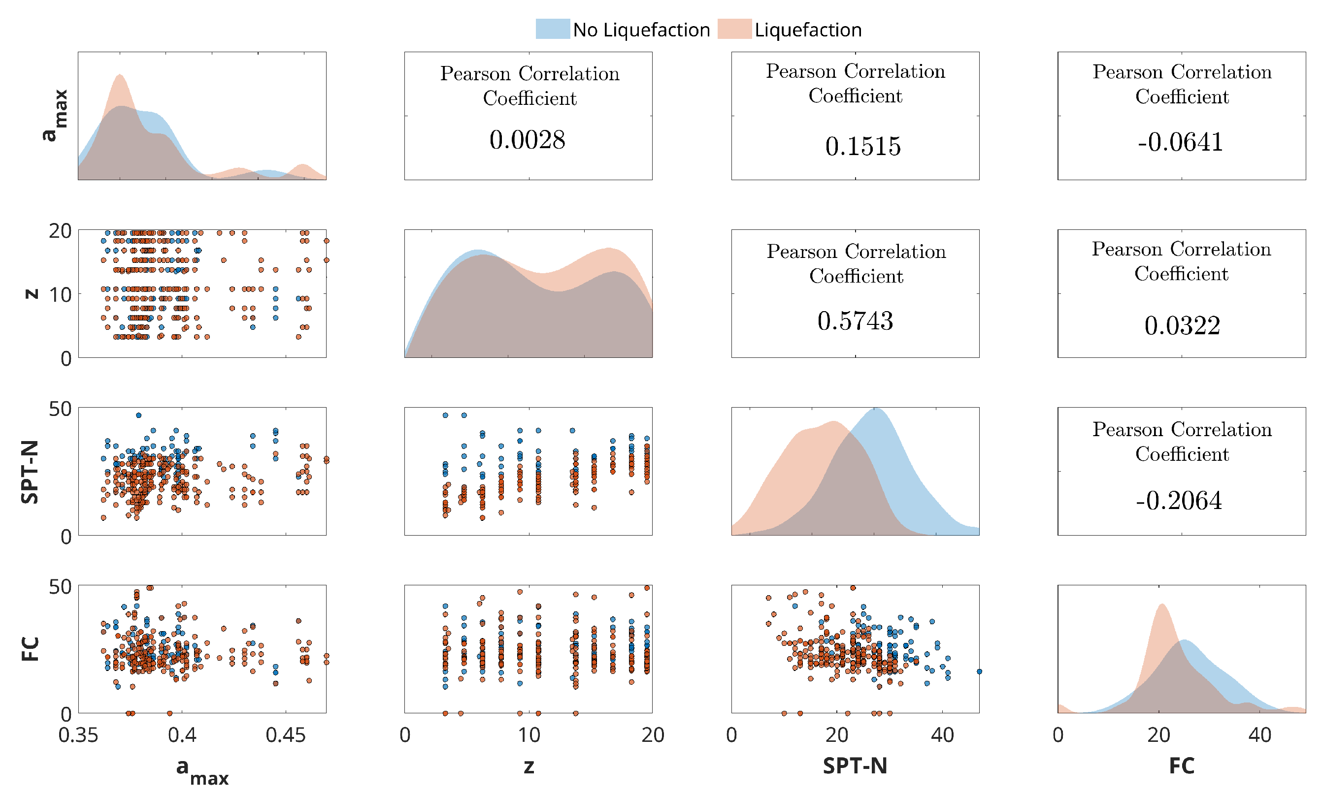
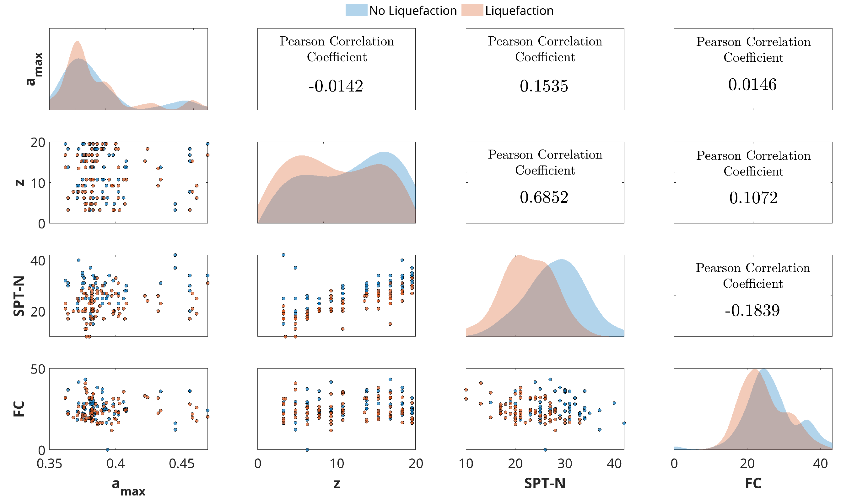
Figure 4 and Figure 5 present the correlation and distribution analysis of the input variables considered for liquefaction prediction in the training and test datasets, respectively. The diagonal elements show the kernel density estimates, where liquefaction cases are most frequently associated with low SPT–N values, moderate fines content (FC), and shallow depths, while peak ground acceleration ( a m a x ) exhibits limited separation between classes. The off-diagonal scatter plots illustrate interactions between variables, highlighting the clustering of liquefaction cases at low SPT–N and intermediate FC values, while the upper off-diagonal elements provide Pearson correlation coefficients (r). In the training dataset, the strongest correlation is observed between depth (z) and SPT–N ( r = 0.574 ), while in the test dataset, the relationship is slightly stronger ( r = 0.685 ). A weak negative correlation between FC and SPT–N persists in both datasets ( r 0.20 ), whereas a m a x remains largely uncorrelated with other inputs. These relationships confirm that SPT–N and FC are the most influential inputs, with z and a m a x contributing complementary information. Similar trends have been reported in previous studies, where in situ resistance and depositional properties were consistently identified as dominant predictors of liquefaction, while seismic demand parameters played a secondary role [43,44].
The optimized hyperparameter settings for the machine learning models are presented in Table 2. These configurations were determined through cross-validation and ensured fair comparison across classifiers. The selected quadratic kernel for the SVM and the cosine distance metric for kNN are consistent with recent geotechnical applications of these models [55,70], while the ANN architecture, consisting of a single hidden layer with 206 neurons and ReLU activation, provided sufficient flexibility without overfitting. The RF model was trained using GentleBoost with 31 learners and a moderate learning rate, a configuration that is computationally efficient but, as shown later, prone to overfitting when applied to limited datasets.
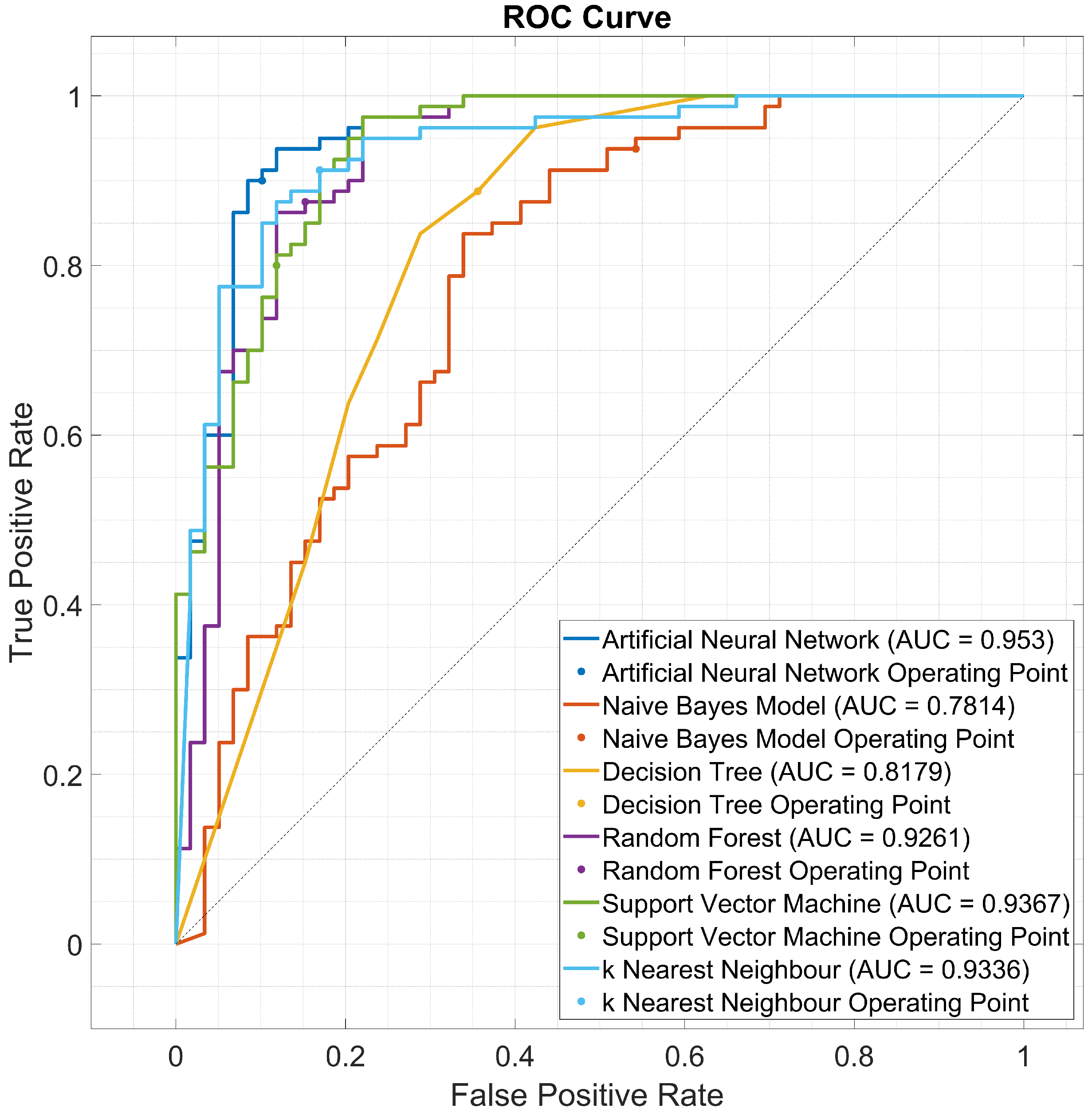
A comparison of predictive performance across all models is shown in Table 3. All classifiers achieved satisfactory results, but their ability to generalize varied considerably. SVM, ANN, and kNN consistently produced the highest and most stable performances. On the test dataset, these models reached accuracies above 93%, with balanced precision and recall in the 93–97% range. ANN achieved the highest area under the ROC curve (AUC = 0.953), while SVM recorded the best test accuracy (94.8%) and a competitive AUC of 0.9367. kNN achieved comparable performance, with an AUC of 0.9336. These results indicate that nonlinear classifiers are particularly effective in capturing the complex boundaries between liquefaction and non-liquefaction conditions.
Comparable outcomes have been documented by Zhou et al. [29,51] and Demir et al. [48,70], who reported that SVM and ANN outperform decision tree models when applied to liquefaction datasets. More recent studies also support these findings by highlighting that classical ML methods such as SVM and ANN remain competitive in moderately sized datasets, even though deep learning approaches like GRU and BiLSTM achieve marginal gains on larger datasets [87].
In comparison, DT and NB achieved moderate classification ability. DT accuracy declined from 89.4% in training to 84.4% in testing, while NB achieved 88.5% test accuracy with high recall (92.8%), indicating its tendency to capture liquefaction cases effectively but with lower precision. RF exhibited strong training performance (96.0%) but dropped to 87.5% in testing, reflecting mild overfitting. Similar issues with ensemble learners under limited sample sizes have been reported in other geotechnical ML studies [56,88]. These results confirm that while tree-based ensembles are powerful, their stability is highly dependent on dataset scale and diversity.
The receiver operating characteristic curves in Figure 6 and Figure 7 further illustrate model separability. ANN demonstrated the strongest discriminatory ability, with an AUC of 0.953, followed by SVM (0.9367) and kNN (0.9336). RF achieved a competitive AUC of 0.926 but was less reliable in generalization, whereas DT (0.818) and NB (0.781) showed weaker decision boundaries. These results confirm the robustness of ANN, SVM, and kNN for practical applications, as they combine high accuracy with balanced sensitivity and specificity.
In addition to classification accuracy, the computation time and convergence characteristics of each model were evaluated to assess their suitability for practical implementation. As summarized in Table 4, ANN achieved the lowest classification error (0.040) but required the longest training time (3407.8 s), and RF exhibited high accuracy (0.050 error) but a longer computation time due to its ensemble nature. SVM offered an excellent trade-off between precision and efficiency, achieving 94.8% test accuracy with a moderate training time (1139.3 s). DT and kNN models provided competitive accuracy of 84.4% and 93.8%, with substantially shorter training durations of 470.4 s and 255.2 s, respectively. Although NB trained quickly, its higher error (0.147) limited its applicability in precision-sensitive analyses. Based on the overall comparison, kNN offers the best balance between computational efficiency and accuracy, followed closely by SVM and DT. For applications requiring rapid, real-time, or large-scale liquefaction assessment, kNN and DT are the most practical models. When higher accuracy and robustness are required and computation time is less critical, SVM, ANN, or RF is preferred.
From a geotechnical perspective, the patterns identified by the models are consistent with empirical observations from past earthquakes, such as the Niigata (1964), Kocaeli (1999), and Canterbury (2010) earthquakes, where liquefaction predominantly occurred in shallow, loose, and moderately fine-grained soils [10,24]. This agreement between model predictions and field evidence enhances confidence in the applicability of ML classifiers for liquefaction hazard assessment. In practical terms, the results highlight three main implications. First, local calibration is crucial: region-specific models, such as those developed for the Edremit basin, offer more reliable predictions than global models trained on heterogeneous datasets. Second, recall should be prioritized in threshold selection due to the severe consequences of false negatives, and models with high AUC values, such as ANN, are particularly suitable for safety-critical decision-making. Third, incorporating additional parameters, including the shear wave velocity, CPT indices, and groundwater data, is expected to further improve predictive robustness.

4. Conclusions

This study applied and compared six machine learning (ML) models—Decision Tree (DT), Naïve Bayes (NB), Support Vector Machine (SVM), k-Nearest Neighbor (kNN), Random Forest (RF), and Artificial Neural Network (ANN)—for prediction of earthquake-induced soil liquefaction in the Edremit settlement area (Balıkesir, NW Turkey), situated along the Edremit Fault Zone, a southern segment of the North Anatolian Fault Zone. The dataset comprised 461 soil layers, with 322 used for training and 139 for testing. Input parameters included peak ground acceleration ( a m a x ), the standard penetration test (SPT-N), depth (z), and fines content (FC), all derived directly from field investigations and the Turkey Earthquake Hazard Map without preprocessing. This ensured that the models were trained on raw geotechnical and seismic data representative of local site conditions.
The results demonstrate that all ML models achieved reasonable predictive capability, though with varying effectiveness. SVM, kNN, and ANN consistently produced the highest performance across all metrics, with test accuracies exceeding 93%. These models demonstrated strong generalization and effectively captured nonlinear interactions between soil resistance parameters and seismic loading. RF also showed high accuracy in training but declined in testing, reflecting sensitivity to dataset size. In contrast, DT and NB, although competitive during training, underperformed on the test set due to overfitting in DT and the simplifying assumptions of NB. Overall, SVM, ANN, and kNN emerged as the most robust classifiers, followed by RF, while DT and NB proved less reliable.
Compared to traditional liquefaction assessment methods based on empirical correlations, such as simplified SPT-based procedures, the ML models offer clear advantages. They can simultaneously account for multiple interacting inputs and uncover nonlinear patterns, thereby reducing both false negatives, which pose safety risks, and false positives, which lead to overly conservative and costly designs. This demonstrates the practical utility of ML for enhancing geotechnical hazard assessment.
Nonetheless, several limitations should be acknowledged. The dataset is geographically restricted to the Edremit basin, limiting the diversity of soil types and seismic conditions considered. The input parameters were restricted to four variables, excluding other potentially influential factors such as the groundwater level, soil plasticity, and stress history. Additionally, the models were evaluated deterministically, without explicit uncertainty quantification, and their interpretability remains limited, which may hinder broader acceptance in engineering practice.
Future research should therefore expand the dataset to include case histories from different geological and seismic environments, incorporate a wider range of predictive features (e.g., groundwater depth, shear wave velocity, CPT indices, and stress history), and employ independent external validation. Advanced ensemble and boosting algorithms such as XGBoost and LightGBM should be explored to enhance predictive performance while reducing overfitting. Furthermore, integrating uncertainty quantification techniques (e.g., Bayesian learning and bootstrapped ensembles) and explainable AI approaches (e.g., SHAP values and feature attribution) can improve reliability and transparency. Hybrid frameworks that combine physics-based liquefaction models with data-driven methods also represent a promising direction. When considered alongside the literature, the present results confirm the growing role of machine learning as a practical and reliable complement to traditional liquefaction evaluation methods in seismically active regions. Addressing current limitations through expanded datasets, enriched feature sets, and interpretable hybrid approaches will be essential for translating these methods into routine geotechnical engineering practice and improving infrastructure resilience in earthquake-prone regions.
In addition, the practical implementation framework developed in this study (Figure 3) demonstrates how the proposed ML models can be systematically integrated into existing seismic hazard assessment workflows. The approach enables rapid, data-driven estimation of soil liquefaction potential using readily available geotechnical and seismic parameters, making it suitable for both regional mapping and real-time applications. This integration enhances the practical utility of ML methods and supports more resilient infrastructure design in seismically active regions.

Author Contributions

Conceptualization, E.C.O. and N.K.C.; methodology, E.C.O.; software, E.C.O.; formal analysis, E.C.O. and N.K.C.; investigation, E.C.O. and N.K.C.; resources, S.C. and N.C.; data curation, N.C. and S.C.; writing—original draft preparation, E.C.O. and N.K.C.; writing—review and editing, E.C.O., N.K.C., N.C. and S.C.; visualization, E.C.O. and N.K.C.; supervision, S.C.; project administration, E.C.O.; funding acquisition, N.C. and S.C. All authors have read and agreed to the published version of the manuscript.

Funding

This research received no external funding.

Institutional Review Board Statement

Not applicable.

Informed Consent Statement

Not applicable.

Data Availability Statement

The data presented in this study are available on request from the corresponding author.

Acknowledgments

The authors gratefully acknowledge the support and cooperation provided by the Scientific Research Projects Coordinator Units (BAP) of Recep Tayyip Erdogan University, Istanbul-Cerrahpaşa University, and Balıkesir University.

Conflicts of Interest

The authors declare no conflicts of interest.

References

  1. Castro, G. On the behavior of soils during earthquakes–liquefaction. Dev. Geotech. Eng. 1987, 42, 169–204. [Google Scholar]
  2. Kumar, A.; Srinivas, B.V. Easy to use empirical correlations for liquefaction and no liquefaction conditions. Geotech. Geol. Eng. 2017, 35, 1383–1407. [Google Scholar] [CrossRef]
  3. Dengiz, O. Soil quality index for paddy fields based on standard scoring functions and weight allocation method. Arch. Agron. Soil Sci. 2020, 66, 301–315. [Google Scholar] [CrossRef]
  4. Youd, T. Ground failure investigations following the 1964 Alaska Earthquake. In Proceedings of the 10th National Conference in Earthquake Engineering, Earthquake Engineering Research Institute, Anchorage, AK, USA, 21–25 July 2014. [Google Scholar]
  5. Ishihara, K.; Koga, Y. Case studies of liquefaction in the 1964 Niigata earthquake. Soils Found. 1981, 21, 35–52. [Google Scholar] [CrossRef] [PubMed]
  6. Seed, R.B.; Dickenson, S.; Idriss, I. Principal geotechnical aspects of the 1989 Loma Prieta earthquake. Soils Found. 1991, 31, 1–26. [Google Scholar] [CrossRef]
  7. Tanaka, Y. The 1995 great Hanshin Earthquake and liquefaction damages at reclaimed lands in Kobe Port. Int. J. Offshore Polar Eng. 2000, 10, ISOPE-00-10-1-064. [Google Scholar]
  8. Chu, D.B.; Stewart, J.P.; Lee, S.; Tsai, J.S.; Lin, P.; Chu, B.; Seed, R.B.; Hsu, S.; Yu, M.; Wang, M.C. Documentation of soil conditions at liquefaction and non-liquefaction sites from 1999 Chi–Chi (Taiwan) earthquake. Soil Dyn. Earthq. Eng. 2004, 24, 647–657. [Google Scholar] [CrossRef]
  9. Erken, A.; Kaya, Z.; Erdem, A. Ground deformations in Adapazari during 1999 Kocaeli Earthquake. In Proceedings of the 13th World Conference on Earthquake Engineering, Vancouver, BC, Canada, 1–6 August 2004; pp. 29–32. [Google Scholar]
  10. Quigley, M.C.; Bastin, S.; Bradley, B.A. Recurrent liquefaction in Christchurch, New Zealand, during the Canterbury earthquake sequence. Geology 2013, 41, 419–422. [Google Scholar] [CrossRef]
  11. Nanda, G.; Mulyani, A. Analysis of landscape changes using high-resolution satellite images at former rice fields after earthquake and liquefaction in Central Sulawesi Province. IOP Conf. Ser. Earth Environ. Sci. 2021, 648, 012203. [Google Scholar] [CrossRef]
  12. Tobita, T.; Kiyota, T.; Torisu, S.; Cinicioglu, O.; Tonuk, G.; Milev, N.; Contreras, J.; Contreras, O.; Shiga, M. Geotechnical damage survey report on February 6, 2023 Turkey-Syria Earthquake, Turkey. Soils Found. 2024, 64, 101463. [Google Scholar] [CrossRef]
  13. Ceryan, S.; Ceryan, N. A new index for microzonation of earthquake prone settlement area by considering liquefaction potential and fault avoidance zone: An example case from Edremit (Balikesir, Turkey). Arab. J. Geosci. 2021, 14, 2216. [Google Scholar] [CrossRef]
  14. Zhao, H.B.; Ru, Z.L.; Yin, S. Updated support vector machine for seismic liquefaction evaluation based on the penetration tests. Mar. Georesources Geotechnol. 2007, 25, 209–220. [Google Scholar] [CrossRef]
  15. Seed, H.B.; Idriss, I.M.; Arango, I. Evaluation of liquefaction potential using field performance data. J. Geotech. Eng. 1983, 109, 458–482. [Google Scholar] [CrossRef]
  16. Idriss, I.; Boulanger, R. Semi-empirical procedures for evaluating liquefaction potential during earthquakes. Soil Dyn. Earthq. Eng. 2006, 26, 115–130. [Google Scholar] [CrossRef]
  17. Johari, A.; Khodaparast, A. Modelling of probability liquefaction based on standard penetration tests using the jointly distributed random variables method. Eng. Geol. 2013, 158, 1–14. [Google Scholar] [CrossRef]
  18. Rahman, M.Z.; Siddiqua, S. Evaluation of liquefaction-resistance of soils using standard penetration test, cone penetration test, and shear-wave velocity data for Dhaka, Chittagong, and Sylhet cities in Bangladesh. Environ. Earth Sci. 2017, 76, 207. [Google Scholar] [CrossRef]
  19. Andrus, R.D.; Stokoe, K.H.; Chung, R.M.; Juang, C.H. Draft Guidelines for Evaluating Liquefaction Resistance Using Shear Wave Velocity Measurements and Simplified Procedures; NIST Interagency/Internal Report (NISTIR); National Institute of Standards and Technology: Gaithersburg, MD, USA, 1999.
  20. Kayen, R.; Moss, R.; Thompson, E.; Seed, R.; Cetin, K.; Kiureghian, A.D.; Tanaka, Y.; Tokimatsu, K. Shear-wave velocity–based probabilistic and deterministic assessment of seismic soil liquefaction potential. J. Geotech. Geoenviron. Eng. 2013, 139, 407–419. [Google Scholar] [CrossRef]
  21. Robertson, P. Comparing CPT and V s liquefaction triggering methods. J. Geotech. Geoenviron. Eng. 2015, 141, 04015037. [Google Scholar] [CrossRef]
  22. Johari, A.; Khodaparast, A.; Javadi, A. An analytical approach to probabilistic modeling of liquefaction based on shear wave velocity. Iran. J. Sci. Technol. Trans. Civ. Eng. 2019, 43, 263–275. [Google Scholar] [CrossRef]
  23. Chen, G.; Wu, Q.; Zhao, K.; Shen, Z.; Yang, J. A binary packing material–based procedure for evaluating soil liquefaction triggering during earthquakes. J. Geotech. Geoenviron. Eng. 2020, 146, 04020040. [Google Scholar] [CrossRef]
  24. Youd, T.L.; Idriss, I.M. Liquefaction resistance of soils: Summary report from the 1996 NCEER and 1998 NCEER/NSF workshops on evaluation of liquefaction resistance of soils. J. Geotech. Geoenviron. Eng. 2001, 127, 297–313. [Google Scholar] [CrossRef]
  25. Juang, C.H.; Yuan, H.; Lee, D.H.; Lin, P.S. Simplified cone penetration test-based method for evaluating liquefaction resistance of soils. J. Geotech. Geoenviron. Eng. 2003, 129, 66–80. [Google Scholar] [CrossRef]
  26. Boulanger, R.W.; Idriss, I. CPT-based liquefaction triggering procedure. J. Geotech. Geoenviron. Eng. 2016, 142, 04015065. [Google Scholar] [CrossRef]
  27. Pal, M. Support vector machines-based modelling of seismic liquefaction potential. Int. J. Numer. Anal. Methods Geomech. 2006, 30, 983–996. [Google Scholar] [CrossRef]
  28. Zhang, J.; Wang, Y. An ensemble method to improve prediction of earthquake-induced soil liquefaction: A multi-dataset study. Neural Comput. Appl. 2021, 33, 1533–1546. [Google Scholar] [CrossRef]
  29. Zhou, J.; Huang, S.; Zhou, T.; Armaghani, D.J.; Qiu, Y. Employing a genetic algorithm and grey wolf optimizer for optimizing RF models to evaluate soil liquefaction potential. Artif. Intell. Rev. 2022, 55, 5673–5705. [Google Scholar] [CrossRef]
  30. Hanna, A.M.; Ural, D.; Saygili, G. Evaluation of liquefaction potential of soil deposits using artificial neural networks. Eng. Comput. 2007, 24, 5–16. [Google Scholar] [CrossRef]
  31. Zhang, X.; He, B.; Sabri, M.M.S.; Al-Bahrani, M.; Ulrikh, D.V. Soil liquefaction prediction based on bayesian optimization and support vector machines. Sustainability 2022, 14, 11944. [Google Scholar] [CrossRef]
  32. Huang, F.K.; Wang, G.S. A Method for Developing Seismic Hazard-Consistent Fragility Curves for Soil Liquefaction Using Monte Carlo Simulation. Appl. Sci. 2024, 14, 9482. [Google Scholar] [CrossRef]
  33. Liu, K.; Hu, X.; Zhou, H.; Tong, L.; Widanage, W.D.; Marco, J. Feature analyses and modeling of lithium-ion battery manufacturing based on random forest classification. IEEE/ASME Trans. Mechatronics 2021, 26, 2944–2955. [Google Scholar] [CrossRef]
  34. Ozkat, E.C.; Abdioglu, M.; Ozturk, U.K. Machine learning driven optimization and parameter selection of multi-surface HTS Maglev. Phys. C Supercond. Its Appl. 2024, 616, 1354430. [Google Scholar] [CrossRef]
  35. Goh, A.T.; Goh, S. Support vector machines: Their use in geotechnical engineering as illustrated using seismic liquefaction data. Comput. Geotech. 2007, 34, 410–421. [Google Scholar] [CrossRef]
  36. Samui, P.; Kim, D.; Sitharam, T. Support vector machine for evaluating seismic-liquefaction potential using shear wave velocity. J. Appl. Geophys. 2011, 73, 8–15. [Google Scholar] [CrossRef]
  37. Karthikeyan, J.; Samui, P. Application of statistical learning algorithms for prediction of liquefaction susceptibility of soil based on shear wave velocity. Geomat. Nat. Hazards Risk 2014, 5, 7–25. [Google Scholar] [CrossRef]
  38. Shahri, A.A. Assessment and prediction of liquefaction potential using different artificial neural network models: A case study. Geotech. Geol. Eng. 2016, 34, 807–815. [Google Scholar] [CrossRef]
  39. Xue, X.; Xiao, M. Application of genetic algorithm-based support vector machines for prediction of soil liquefaction. Environ. Earth Sci. 2016, 75, 874. [Google Scholar] [CrossRef]
  40. Ahmad, M.; Tang, X.W.; Qiu, J.N.; Ahmad, F. Evaluating seismic soil liquefaction potential using bayesian belief network and C4. 5 decision tree approaches. Appl. Sci. 2019, 9, 4226. [Google Scholar] [CrossRef]
  41. Rahbarzare, A.; Azadi, M. Improving prediction of soil liquefaction using hybrid optimization algorithms and a fuzzy support vector machine. Bull. Eng. Geol. Environ. 2019, 78, 4977–4987. [Google Scholar] [CrossRef]
  42. Hu, J.; Liu, H. Bayesian network models for probabilistic evaluation of earthquake-induced liquefaction based on CPT and Vs databases. Eng. Geol. 2019, 254, 76–88. [Google Scholar] [CrossRef]
  43. Zhang, Y.; Qiu, J.; Zhang, Y.; Xie, Y. The adoption of a support vector machine optimized by GWO to the prediction of soil liquefaction. Environ. Earth Sci. 2021, 80, 360. [Google Scholar] [CrossRef]
  44. Liu, L.; Zhang, S.; Yao, X.; Gao, H.; Wang, Z.; Shen, Z. Liquefaction evaluation based on shear wave velocity using random forest. Adv. Civ. Eng. 2021, 2021, 3230343. [Google Scholar] [CrossRef]
  45. Zhao, Z.; Duan, W.; Cai, G. A novel PSO-KELM based soil liquefaction potential evaluation system using CPT and Vs measurements. Soil Dyn. Earthq. Eng. 2021, 150, 106930. [Google Scholar] [CrossRef]
  46. Zhang, Y.; Xie, Y.; Zhang, Y.; Qiu, J.; Wu, S. The adoption of deep neural network (DNN) to the prediction of soil liquefaction based on shear wave velocity. Bull. Eng. Geol. Environ. 2021, 80, 5053–5060. [Google Scholar] [CrossRef]
  47. Kumar, D.; Samui, P.; Kim, D.; Singh, A. A novel methodology to classify soil liquefaction using deep learning. Geotech. Geol. Eng. 2021, 39, 1049–1058. [Google Scholar] [CrossRef]
  48. Demir, S.; Şahin, E.K. Liquefaction prediction with robust machine learning algorithms (SVM, RF, and XGBoost) supported by genetic algorithm-based feature selection and parameter optimization from the perspective of data processing. Environ. Earth Sci. 2022, 81, 459. [Google Scholar] [CrossRef]
  49. Ozsagir, M.; Erden, C.; Bol, E.; Sert, S.; Özocak, A. Machine learning approaches for prediction of fine-grained soils liquefaction. Comput. Geotech. 2022, 152, 105014. [Google Scholar] [CrossRef]
  50. Hanandeh, S.M.; Al-Bodour, W.A.; Hajij, M.M. A comparative study of soil liquefaction assessment using machine learning models. Geotech. Geol. Eng. 2022, 40, 4721–4734. [Google Scholar] [CrossRef]
  51. Zhou, J.; Huang, S.; Wang, M.; Qiu, Y. Performance evaluation of hybrid GA–SVM and GWO–SVM models to predict earthquake-induced liquefaction potential of soil: A multi-dataset investigation. Eng. Comput. 2022, 38, 4197–4215. [Google Scholar] [CrossRef]
  52. Duan, W.; Zhao, Z.; Cai, G.; Wang, A.; Wu, M.; Dong, X.; Liu, S. V s-based assessment of soil liquefaction potential using ensembling of GWO–KLEM and Bayesian theorem: A full probabilistic design perspective. Acta Geotech. 2023, 18, 1863–1881. [Google Scholar] [CrossRef]
  53. Sui, Q.R.; Chen, Q.H.; Wang, D.D.; Tao, Z.G. Application of machine learning to the V s-based soil liquefaction potential assessment. J. Mt. Sci. 2023, 20, 2197–2213. [Google Scholar] [CrossRef]
  54. Yang, Y.; Wei, Y. Study on Classification Method of Soil Liquefaction Potential Based on Decision Tree. Appl. Sci. 2023, 13, 4459. [Google Scholar] [CrossRef]
  55. Abbasimaedeh, P. Soil liquefaction in seismic events: Pioneering predictive models using machine learning and advanced regression techniques. Environ. Earth Sci. 2024, 83, 189. [Google Scholar] [CrossRef]
  56. Ghani, S.; Thapa, I.; Kumari, S.; Correia, A.G.; Asteris, P.G. Revealing the nature of soil liquefaction using machine learning. Earth Sci. Inform. 2025, 18, 198. [Google Scholar] [CrossRef]
  57. Zhang, S.; Li, X.; Zong, M.; Zhu, X.; Wang, R. Efficient kNN classification with different numbers of nearest neighbors. IEEE Trans. Neural Netw. Learn. Syst. 2017, 29, 1774–1785. [Google Scholar] [CrossRef] [PubMed]
  58. Ozkat, E.C. A method to classify steel plate faults based on ensemble learning. J. Mater. Mechatronics A 2022, 3, 240–256. [Google Scholar] [CrossRef]
  59. Guo, H.; Zhuang, X.; Chen, J.; Zhu, H. Predicting earthquake-induced soil liquefaction based on machine learning classifiers: A comparative multi-dataset study. Int. J. Comput. Methods 2022, 19, 2142004. [Google Scholar] [CrossRef]
  60. Gandomi, A.H.; Fridline, M.M.; Roke, D.A. Decision tree approach for soil liquefaction assessment. Sci. World J. 2013, 2013, 346285. [Google Scholar] [CrossRef]
  61. Ahmad, M.; Tang, X.W.; Qiu, J.N.; Ahmad, F.; Gu, W.J. Application of machine learning algorithms for the evaluation of seismic soil liquefaction potential. Front. Struct. Civ. Eng. 2021, 15, 490–505. [Google Scholar] [CrossRef]
  62. Ekinci, Y.L.; Yiğitbaş, E. A geophysical approach to the igneous rocks in the Biga Peninsula (NW Turkey) based on airborne magnetic anomalies: Geological implications. Geodin. Acta 2012, 25, 267–285. [Google Scholar] [CrossRef]
  63. Sozbilir, H.; Ozkaymak, C.; Uzel, B.; Sumer, O. Criteria for Surface Rupture Microzonation of Active Faults for Earthquake Hazards in Urban Areas. In Handbook of Research on Trends and Digital Advances in Engineering Geology; IGI Global: Hershey, PA, USA, 2018; pp. 187–230. [Google Scholar]
  64. Ceryan, S.; Samui, P.; Ozkan, O.S.; Berber, S.; Tudes, S.; Elci, H.; Ceryan, N. Soil liquefaction susceptibility of Akcay residential area (Biga Peninsula, Turkey) close to North Anatolian fault zone. J. Min. Environ. 2023, 14, 1141–1153. [Google Scholar]
  65. Sozbilir, H.; Sumer, O.; Ozkaymak, C.; Uzel, B.; Guler, T.; Eski, S. Kinematic analysis and palaeoseismology of the Edremit Fault Zone: Evidence for past earthquakes in the southern branch of the North Anatolian Fault Zone, Biga Peninsula, NW Turkey. Geodin. Acta 2016, 28, 273–294. [Google Scholar] [CrossRef]
  66. Alsan, E.; Tezuçan, L.; Bath, M. An earthquake catalogue for Turkey for the interval 1913–1970. Tectonophysics 1976, 31, T13–T19. [Google Scholar] [CrossRef]
  67. Tsuchida, H. Prediction and countermeasure against the liquefaction in sand deposits. In Abstract of the Seminar in the Port and Harbor Research Institute; Scientific Research Publishing: Wuhan, China, 1970; pp. 31–333. [Google Scholar]
  68. Javanbakht, A.; Molnar, S.; Sadrekarimi, A.; Adhikari, S.R. Performance-based liquefaction analysis and probabilistic liquefaction hazard mapping using CPT data within the Fraser River delta, Canada. Soil Dyn. Earthq. Eng. 2025, 189, 109101. [Google Scholar] [CrossRef]
  69. Kamal, A.M.; Sahebi, M.T.; Hossain, M.S.; Rahman, M.Z.; Fahim, A.K.F. Liquefaction hazard mapping of the south-central coastal areas of Bangladesh. Nat. Hazards Res. 2024, 4, 520–529. [Google Scholar] [CrossRef]
  70. Demir, S.; Sahin, E.K. The effectiveness of data pre-processing methods on the performance of machine learning techniques using RF, SVR, Cubist and SGB: A study on undrained shear strength prediction. Stoch. Environ. Res. Risk Assess. 2024, 38, 3273–3290. [Google Scholar] [CrossRef]
  71. Dastjerdy, B.; Saeidi, A.; Heidarzadeh, S. Review of applicable outlier detection methods to treat geomechanical data. Geotechnics 2023, 3, 375–396. [Google Scholar] [CrossRef]
  72. Ozkat, E.C. Photodiode Signal Patterns: Unsupervised Learning for Laser Weld Defect Analysis. Processes 2025, 13, 121. [Google Scholar] [CrossRef]
  73. Ozkat, E.C.; Franciosa, P.; Ceglarek, D. A framework for physics-driven in-process monitoring of penetration and interface width in laser overlap welding. Procedia CIRP 2017, 60, 44–49. [Google Scholar] [CrossRef]
  74. Shao, W.; Yue, W.; Zhang, Y.; Zhou, T.; Zhang, Y.; Dang, Y.; Wang, H.; Feng, X.; Chao, Z. The application of machine learning techniques in geotechnical engineering: A review and comparison. Mathematics 2023, 11, 3976. [Google Scholar] [CrossRef]
  75. Wang, G.; Zhao, B.; Wu, B.; Zhang, C.; Liu, W. Intelligent prediction of slope stability based on visual exploratory data analysis of 77 in situ cases. Int. J. Min. Sci. Technol. 2023, 33, 47–59. [Google Scholar] [CrossRef]
  76. Walters-Williams, J.; Li, Y. Comparative study of distance functions for nearest neighbors. In Advanced Techniques in Computing Sciences and Software Engineering; Springer: Berlin/Heidelberg, Germany, 2010; pp. 79–84. [Google Scholar]
  77. Kramer, O. Dimensionality Reduction with Unsupervised Nearest Neighbors; Springer: Berlin/Heidelberg, Germany, 2013; Volume 51. [Google Scholar]
  78. Rolnick, D.; Donti, P.L.; Kaack, L.H.; Kochanski, K.; Lacoste, A.; Sankaran, K.; Ross, A.S.; Milojevic-Dupont, N.; Jaques, N.; Waldman-Brown, A.; et al. Tackling climate change with machine learning. Acm Comput. Surv. (CSUR) 2022, 55, 1–96. [Google Scholar] [CrossRef]
  79. Güner, E.; Özkan, Ö.; Yalcin-Ozkat, G.; Ölgen, S. Determination of novel SARS-CoV-2 inhibitors by combination of machine learning and molecular modeling methods. Med. Chem. 2024, 20, 153–231. [Google Scholar] [CrossRef] [PubMed]
  80. Özkat, G.Y.; Aasim, M.; Bakhsh, A.; Ali, S.A.; Özcan, S. Machine learning models for optimization, validation, and prediction of light emitting diodes with kinetin based basal medium for in vitro regeneration of upland cotton (Gossypium hirsutum L.). J. Cotton Res. 2025, 8, 19. [Google Scholar] [CrossRef]
  81. Chala, A.T.; Ray, R. Assessing the performance of machine learning algorithms for soil classification using cone penetration test data. Appl. Sci. 2023, 13, 5758. [Google Scholar] [CrossRef]
  82. Pradhan, B. A comparative study on the predictive ability of the decision tree, support vector machine and neuro-fuzzy models in landslide susceptibility mapping using GIS. Comput. Geosci. 2013, 51, 350–365. [Google Scholar] [CrossRef]
  83. He, Q.; Xu, Z.; Li, S.; Li, R.; Zhang, S.; Wang, N.; Pham, B.T.; Chen, W. Novel entropy and rotation forest-based credal decision tree classifier for landslide susceptibility modeling. Entropy 2019, 21, 106. [Google Scholar] [CrossRef]
  84. Kumar, D.R.; Samui, P.; Burman, A. Prediction of probability of liquefaction using soft computing techniques. J. Inst. Eng. (India) Ser. A 2022, 103, 1195–1208. [Google Scholar] [CrossRef]
  85. Ceryan, N.; Ozkat, E.C.; Korkmaz Can, N.; Ceryan, S. Machine learning models to estimate the elastic modulus of weathered magmatic rocks. Environ. Earth Sci. 2021, 80, 448. [Google Scholar] [CrossRef]
  86. Ikram, N.; Basharat, M.; Ali, A.; Usmani, N.A.; Gardezi, S.A.H.; Hussain, M.L.; Riaz, M.T. Comparison of landslide susceptibility models and their robustness analysis: A case study from the NW Himalayas, Pakistan. Geocarto Int. 2022, 37, 9204–9241. [Google Scholar] [CrossRef]
  87. Şehmusoğlu, E.H.; Kurnaz, T.F.; Erden, C. Estimation of soil liquefaction using artificial intelligence techniques: An extended comparison between machine and deep learning approaches. Environ. Earth Sci. 2025, 84, 130. [Google Scholar] [CrossRef]
  88. Onyelowe, K.C.; Kamchoom, V.; Gnananandarao, T.; Arunachalam, K.P. Developing data driven framework to model earthquake induced liquefaction potential of granular terrain by machine learning classification models. Sci. Rep. 2025, 15, 21509. [Google Scholar] [CrossRef]
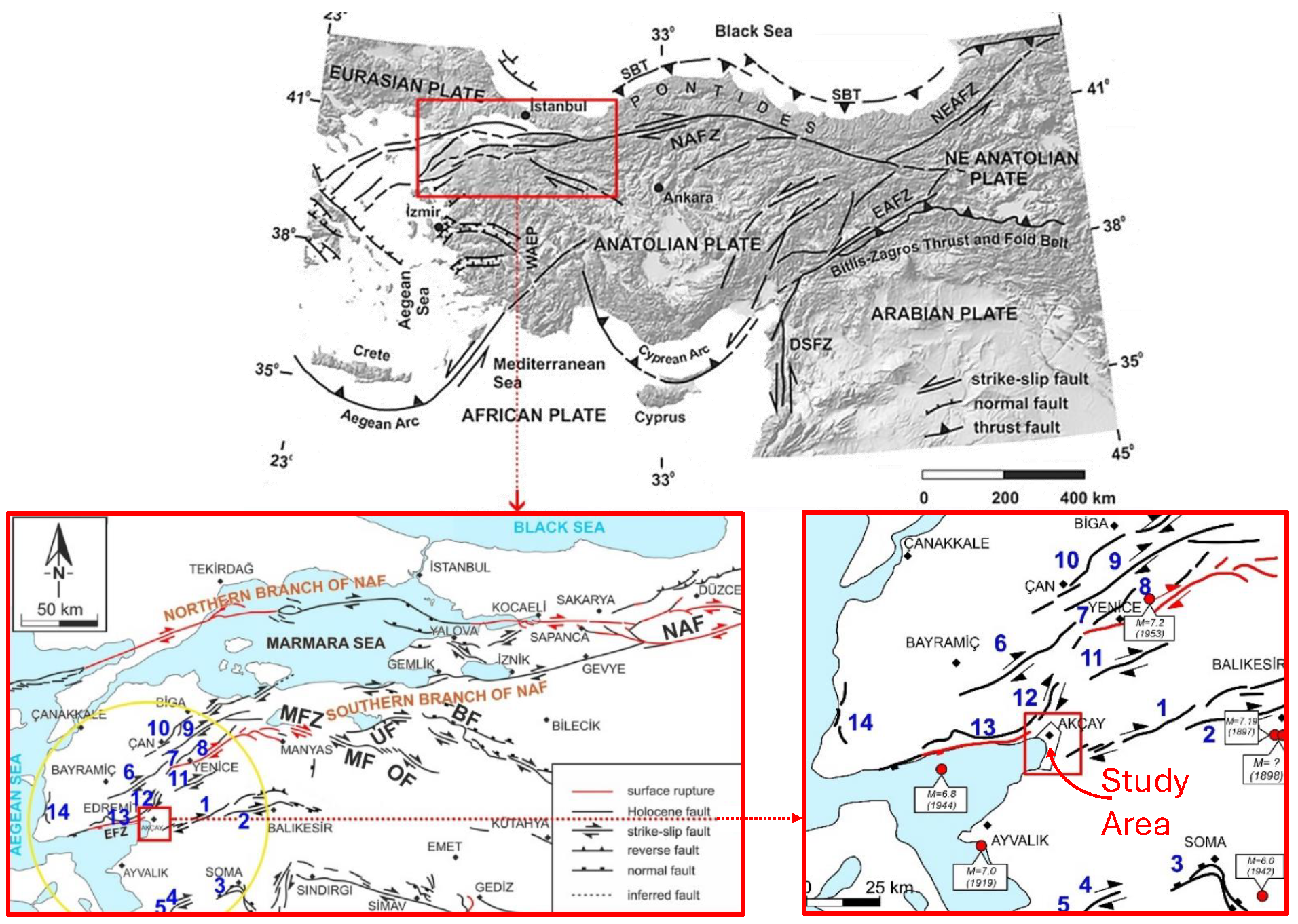
Figure 1. Simplified neotectonic framework and active fault map of northwestern Anatolia, where the red-boxed inset maps precisely indicate the location of the study area. NAF: North Anatolian Fault; BF: Bursa Fault; UF: Ulubat Fault; MF: Mustafakemalpaşa Fault; OF: Orhangazi Fault; MFZ: Manyas Fault Zone. (1) Havran–Balya Fault; (2) Balıkesir Fault; (3) Soma–Kırkağaç Fault Zone; (4) Bergama Fault; (5) Zeytindağ Fault Zone; (6) Evciler Fault; (7) Bekten Fault; (8) Yenice–Gönen Fault; (9) Sarıköy Fault; (10) Biga–Çan Fault Zone; (11) Pazarköy Fault; (12) Altınoluk segment of the Edremit Fault Zone (EFZ); (13) Zeytinli segment of the EFZ; (14) Kestanbol Fault (modified after [62,63,64]).
Applsci 15 11512 g001
Figure 2. Graph of liquefaction potential level based on grain gradation [67] and the different soil types defined in the soil layers of the alluvium in the study area [64].
Applsci 15 11512 g002
Figure 3. Workflow representing the methodology of the present study for predicting soil liquefaction potential using machine learning.
Applsci 15 11512 g003
Figure 4. Correlation among inputs for training dataset categorized according to soil liquefaction.
Applsci 15 11512 g004
Figure 5. Correlation among inputs for test dataset categorized according to soil liquefaction.
Applsci 15 11512 g005
Figure 6. ROC curve and AUC points for each ML model for the training dataset.
Applsci 15 11512 g006
Figure 7. ROC curve and AUC points for each ML model for the testing dataset.
Applsci 15 11512 g007
Table 1. Summary of input parameters in machine learning models for assessment of soil liquefaction.
ReferenceML Model(s)Dataset of Soil
Liquefaction Evaluation
Inputs
[35]SVMCPT M w , q c , a m a x , σ ´ v o , σ v o , R f
[36]SVM V S M w , a m a x , σ ´ v o , V S , soil type
[37]LSSVM and RVM V S a m a x , V S
[38]ANNSPT, V S σ ´ v o , σ v o , V S , r d , γ , FC, z, N,
CSR, CRR, U, soil type
[39]GA-SVMCPT M w , q c , a m a x , σ ´ v o , σ v o , D 50 , CSR
[40]BBN and DTCPT M w , a m a x , σ ´ v o , σ v o , q c 1 N c s , r r u p , T s ,
I c , FC, D w , Ds
[41]PSO/GA/Fuzzy-SVMCPT M w , q c , a m a x , σ ´ v o , σ v o , D 50 , CSR
[42]BNMSPT, CPT, V S M w , a r m s , z, GWT
[43]DNNSPT, V S M w , a m a x , σ ´ v o , σ v o , V S , ( N 1 ) 60 , FC, z
[44]RM V S M w , a m a x , V S 1 , k
[45]PSO-KELMCPT, V S M w , a m a x , σ ´ v o , σ v o , V S 1 ,
q c 1 N c s , F r , FC, ST, CSR
[46]GWO-SVMSPT, V S M w , a m a x , σ ´ v o , σ v o , V S , ( N 1 ) 60 , FC, z
[47]DL and EmBPCPT q c , a m a x
[48]SVM, RF, andXGBoost V S M w , a m a x , σ ´ v o , σ v o , V S , D w , r d , CSR
[49]DT, LR, SVM, kNN, SGD, RF, and ANNCPTC%, w n , w L , IP, D 50 , FC, z
[50]SVM, DT, and QDACPT M w , q c , q c 1 , D 50 , CSR
[51]GA-SVM and GWO-SVMSPT, V S , CPT M w , q c , a m a x , σ ´ v o , σ v o , R f , V S 1 ,
( N 1 ) 60 , ϕ , α t , s w d , D w , CSR, FC
[52]GA V S M w , a m a x , σ ´ v o , σ v o , V S 1
[53]LDA, QDA, NB, ANN, and CT
SVM, RM, LightGBM, and XGBoost
V S a m a x , σ ´ v o , σ v o , V S 1 , r d , D s , CSR
[54]LR and DT V S M w , a m a x , σ v o , D w , T s , FC, z,
Compactness, gradation, age
[55]LR, RF, and SVMSPT, V S M w , ( N 1 ) 60 , V S , D 50 , FC
[56]GBR, XGB, RF, and DTSPT ( N 1 ) 60 , CSR, PGA, FC, r d
Abbreviations: BBN: Bayesian Belief Network; BNM: Bayesian Network Model; DT: Decision Tree; PSO: Particle Swarm Optimization; GWO: Grey Wolf Optimization; KELM: Kernel Extreme Learning Machine; DNN: Deep Neural Network; LDA: Linear Discriminant Analysis; QDA: Quadratic Discriminant Analysis; NB: Naive Bayes; kNN: K-Nearest Neighbor; ANN: Artificial Neural Network; CT: Classification Tree; SVM: Support Vector Machine; RF: Random Forest; LightGBM: Light Gradient Boosting Machine; XGBoost: Extreme Gradient Boosting; LR: Logistic Regression; SGD: Stochastic Gradient Descent; GA: Genetic Algorithm; LSSVM: Least Squares Support Vector Machine; RVM: Relevance Vector Machine; DL: Deep Learning; EmBP: Emotional Backpropagation Neural Network; M w : earthquake magnitude; a m a x : peak ground acceleration; r r u p : closest distance to rupture surface; FC: fines content; q c 1 N c s : equivalent clean sand normalized cone-tip resistance; q c : cone-tip resistance; q c 1 : normalized cone-tip resistance; R f : sleeve friction ratio; σ ´ v o : vertical effective stress; σ v o : vertical total stress; I c : soil behavior type index; D w : groundwater table depth; D s : depth of soil deposit; T s : thickness of soil layer; GWT: groundwater table; a r m s : root-mean-square acceleration; N: standard penetration blow number; ( N 1 ) 60 : corrected standard penetration blow number; V S : shear wave velocity; V S 1 : normalized shear wave velocity; z: depth of target stratum; F r : normalized friction ratio; ST: soil behavior type determined by the soil behavior type chart, CSR: Cyclic stress ratio; r d : stress reduction coefficient; k: stress ratio; w L : liquid limit; C%: clay content; w n : water content; IP: plasticity index; D 50 : average grain size; ϕ : initial soil friction angle; α t : threshold acceleration; s w d : nonlinear shear mass participation factor; γ : unit weight; U: pore pressure; SPT: standard penetration test.
Table 2. Optimized hyperparameter settings for ML models.
ML ModelParametersValue
DTNumber of splits18
NBDistribution namesGaussian
SVMKernel functionQuadratic
Box constraint level0.3192
kNNNumber of neighbors10
Distance metricCosine
Distance weightSquared inverse
RFEnsemble methodGentleBoost
Number of learners31
Learning rate0.1189
ANNActivation functionReLU
Lambda 3.48 × 10 7
Number of hidden layers1
Number of neurons206
Table 3. Performance comparisons of the models.
ML ModelAccuracyPrecisionRecallF1 Score
TrainTestTrainTestTrainTestTrainTest
DT89.4%84.4%90.5%91.4%92.7%89.5%95.0%87.7%
NB85.4%88.5%85.5%88.8%90.3%92.8%95.6%97.3%
SVM97.8%94.8%97.0%93.6%98.5%96.7%100.0%100.0%
kNN95.1%93.8%94.6%93.5%96.6%96.0%98.8%98.6%
RF96.0%87.5%95.8%91.8%97.2%91.8%98.8%91.8%
ANN96.5%93.8%96.9%93.5%97.5%96.0%98.1%98.6%
Table 4. Computational performance comparison of machine learning models.
ML ModelTraining Time (s)Min. Classification ErrorIterations to Min. Error
DT470.40.10267
NB1177.60.1477
SVM1139.30.04497
kNN255.20.05366
RF3249.80.0507
ANN3407.80.0405
Disclaimer/Publisher’s Note: The statements, opinions and data contained in all publications are solely those of the individual author(s) and contributor(s) and not of MDPI and/or the editor(s). MDPI and/or the editor(s) disclaim responsibility for any injury to people or property resulting from any ideas, methods, instructions or products referred to in the content.