Article

Single-Pass CNN–Transformer for Multi-Label 1H NMR Flavor Mixture Identification

Department of Agricultural Technology, Center for Precision Agriculture, Norwegian Institute of Bioeconomy Research (NIBIO), Nylinna 226, NO-2849 Kapp, Norway
*
Author to whom correspondence should be addressed.
Appl. Sci. 2025, 15(21), 11458; https://doi.org/10.3390/app152111458
Submission received: 3 October 2025 / Revised: 24 October 2025 / Accepted: 25 October 2025 / Published: 27 October 2025

Featured Application

The proposed Hybrid enables single-pass identification of multiple flavor components from 1H NMR spectra, supporting QA/QC (label verification, swap/contamination detection), formulation screening, and incoming-goods inspection. Open-set multi-label outputs allow abstention/flagging of non-library compounds. The compact model (~0.47 M parameters) runs in ~0.68 ms on GPU (V100), facilitating on-premises batch triage with or without GPUs. The workflow generalizes to food authenticity testing and targeted metabolomics.

Abstract

Interpreting multi-component 1H NMR spectra is difficult due to peak overlap, concentration variability, and low-abundance signals. We cast mixture identification as a single-pass multi-label task. A compact CNN–Transformer (“Hybrid”) model was trained end-to-end on domain-informed and realistically simulated spectra derived from a 13-component flavor library; the model requires no real mixtures for training. On 16 real formulations, the Hybrid attains micro-F1 = 0.990 and exact-match (subset) accuracy = 0.875, outperforming CNN-only and Transformer-only ablations, while remaining efficient (~0.47 M parameters; ~0.68 ms on GPU, V100). The approach supports abstention and shows robustness to simulated outsiders. Although the evaluation set was small, and the macro-ECE (per-class, 15 bins) was inflated by sparse classes (≈0.70), the micro-averaged Brier is low (0.0179), and temperature scaling had negligible effect (T ≈ 1.0), indicating the good overall probability quality. The pipeline is readily extensible to larger libraries and adjacent applications in food authenticity and targeted metabolomics. Classical chemometric baselines trained on simulation failed to transfer to real measurements (subset accuracy 0.00), while the Hybrid model maintained strong performance.

1. Introduction

Accurately decomposing nuclear magnetic resonance (NMR) spectra of multi-component mixtures remains challenging in practice: overlapping multiplets, concentration-dependent linewidth and intensity variations, and chemical-shift drift/warping routinely defeat template matching and per-component heuristics [1]. In food chemistry and metabolomics, where spectra are used for compositional profiling, authenticity verification, and contaminant screening, practical workflows require models that reason over the entire spectrum and predict all present components jointly, not one at a time [2,3,4,5,6]. Despite the rich structural information in the fingerprint region, mixture deconvolution remains constrained by these sources of spectral variability [7,8,9].
Conventional approaches to NMR spectral interpretation, manual peak assignment and classical chemometrics, are labor-intensive and scale poorly to complex mixtures. Learning-based methods have begun to address these issues. Pairwise binary formulations such as DeepMID [9] use convolutional neural networks (CNNs) to evaluate the presence of each component separately, and later variants, FlavorFormer [10], which combines CNNs with a Transformer, keep the same per-component evaluation paradigm. While conceptually simple, this pairwise setup has important limitations: (i) inference must be repeated for each library reference (O(C) comparisons), (ii) inter-class dependencies (co-occurrence/exclusion) are not modeled, because decisions are made independently per component, and (iii) architectures that rely solely on CNNs have limited capacity to capture long-range relationships across the spectrum; even when attention is added, the pairwise formulation still does not perform joint multi-label reasoning over all components.
To address these limitations, we present a unified multi-label classification framework for 1H NMR-based flavor analysis using a hybrid CNN and Transformer architecture. Our model jointly predicts all flavor components in a single pass, learning to recognize interactions among them. The CNN layers efficiently extract local spectral features and reduce dimensionality, while the Transformer encoder captures global dependencies. This hybrid approach enables accurate decomposition of overlapping signals and improves model scalability.
We hypothesize that a compact single-pass CNN–Transformer trained only on realistically simulated spectra can generalize to real mixtures without using real-mixture training data, achieving high micro-F1 and exact-match accuracy. To test this, we evaluate real-set accuracy, ablations, calibration, and robustness.

2. Materials and Methods

2.1. Flavor Library and Formulated Flavor Mixtures

Thirteen open-source plant-derived flavor compounds were selected as the reference component library (Table 1). These reference spectra, originally curated and published in the DeepMID study [9], were used to generate both synthetic training data and validate model predictions. Each plant-based flavor was prepared according to standard NMR protocols: the compounds were dissolved in a 1:1 mixture of methanol-d4 (CH3OD) and phosphate buffer (pH-adjusted), vortexed, ultrasonicated, and centrifuged to remove particulates. The resulting supernatant was analyzed using a 600 MHz Bruker Avance NMR spectrometer equipped with a Prodigy cryoprobe. Spectra were acquired under standardized conditions: 128 scans, water suppression using the noesypprld pulse sequence, and a spectral width of 12 ppm. Although real data were acquired on the same spectrometer, the results can vary with measurement protocol (pulse program, temperature, shimming, receiver gain, number of scans, windowing/apodization). Our claims therefore pertain to similar acquisition settings; cross-protocol generalization is evaluated indirectly via the simulation ranges (Section 2.3) and left for larger prospective studies. Representative 1H NMR spectra of all 13 individual flavor components are shown in Figure S1.
In addition to individual components, 16 realistic flavor mixtures—comprising two to five components—were prepared and measured by the same instrument for model evaluation ratios (Table S2 in DeepMID study [9]). The mixtures, including dilution levels and acquisition parameters, follow the experimental specifications reported in the DeepMID study [9]. All spectra were normalized by their maximum intensity to have a maximum value of 1.0 following acquisition to ensure comparability across dilution levels. These 16 formulated mixtures are provided in Figure S2.
During cross-referencing with the DeepMID study, we identified two inconsistencies in the reported labels of test mixtures. Based on spectral overlays and mixture reconstruction, the first mixture is more consistent with components 3 and 8, while the second appears to contain components 3 and 5. We corrected these misannotations for evaluation to ensure accurate ground truth comparisons.

2.2. Model Architecture

We adopt a CNN–Transformer (“Hybrid”) architecture (Figure 1) for single-pass multi-label decomposition of 1H NMR mixtures. A 1D CNN stack (5 layers) with group normalization and strided convolution + max-pooling first captures localized peak/multiplet features and reduces the sequence length. The resulting feature sequence is processed by a Transformer encoder (4 layers, 4 heads, d model = 128 , dropout = 0.1) to model long-range dependencies and spectral context across the full ppm range. A linear classifier head, consisting of two fully connected layers with ReLU activation and dropout = 0.2, with sigmoid outputs produces a 13-dimensional vector of class probabilities (one per flavor component).
From an input of 32,724 points, the CNN stack downsamples to 64 tokens × 128 channels, which are then passed to the Transformer. The CNN front-end (strided 1D convs with GN) reduces 32,724 points to 64 × 128 tokens and captures local line-shape/multiplet cues, improving the SNR and lowering the Transformer’s sequence length. A 4-layer 4-head Transformer (d_model = 128) models the long-range co-occurrence/exclusion across ppm regions. The effective token count is determined solely by CNN strides and pooling; legacy hyperparameters (e.g., transformer_seq_len = 750) are not used at runtime. This design yields constant-time (O(1)) single-pass inference with respect to the library size and explicitly combines local (CNN) and global (Transformer) cues for mixture decoding.

2.3. Synthetic Mixture Generation and Augmentations

From the 13 reference spectra (32,724 points), we generated mixtures as follows. We sampled K in {2, 3, 4, 5} with p ( K ) 13 K 0.8 and then the K component indices uniformly without replacement. The ratios were equal with probability 0.80; otherwise, they were drawn from a Dirichlet with α { 0.5,1.0,2.0 } . The clean mixture (weighted sum) was perturbed to mimic acquisition effects: small axis offsets/warps and stretches, dilution scaling, modest line-broadening, and phase jitter, low-order baseline, ripple, and additive white/low-frequency noise. Simulation ranges were chosen to bracket routine protocol variation, including chemical-shift drift/warp, lineshape/linewidth changes, baseline ripple, SNR/dilution changes, and mild phase errors—factors commonly affected by temperature, shimming, receiver gain, and pulse-sequence differences. With probability 0.5, global polarity was flipped; the labels are polarity-invariant. We applied robust magnitude normalization (90th-percentile division in 80% of cases; max-based otherwise). Presence/absence was defined by an effective magnitude threshold τ pres = 0.01 ; targets y were normalized over present components. We fixed independent seeds for discrete design vs. continuous artifacts for determinism. Each run used 30,000 mixtures split 80/20 for training/validation. More detailed parameters for the spectrum simulation can be found in Table 2. A schematic overview of the data-simulation workflow, from pure component spectra to augmented mixtures, is provided in Supplementary Figure S3.
We assessed realism via nearest-neighbor Pearson correlation between each real spectrum (REAL) and the simulated pool (SIM; median 0.901; IQR 0.813–0.942). We also checked the SIM–REAL overlap using PCA and UMAP plots. We standardized spectra using a SIM-fit StandardScaler and fit the PCA (randomized SVD, 10 comps) and UMAP (n_neighbors = 30, min_dist = 0.1, cosine) on the SIM only; REAL was then projected using the fitted transforms (no leakage). PCA panels (PC1–PC2, PC2–PC3) and a 2D UMAP embedding show REAL embedded within the SIM cloud (Figures S4 and S5).

2.4. Evaluation Metrics (Multilabel) and Threshold Policy

We fixed a global decision threshold of τ = 0.70 for all classes, chosen a priori based on tolerance for false positives; it was not tuned on validation or test data. Unless otherwise noted, all reported results use this threshold.
For multi-label predictions p [ 0 ,   1 ] C and binary targets y { 0 ,   1 } C , we derived binary decisions y ^ = 1   [ p τ ] . The performance was assessed using element-wise accuracy (micro-accuracy), i.e., proportion of correctly predicted labels across all elements:
Micro - F 1 = 2 × c T P c 2 × c T P c + c F P c + c F N c ; subset accuracy (exact match): proportion of spectra with all labels exactly correct: Subset   Accuracy = 1 N i = 1 N 1 ( Y ^ i = Y i ) ; F1-scores: sample-averaged, macro-averaged, and micro-averaged; Jaccard (IoU): macro- and micro-averaged; calibration metrics: Expected Calibration Error (ECE; 15 bins) and mean Brier score across classes. The ECE was computed element-wise over raw per-class probabilities, with 15 equal-width bins.

2.5. Chemometric Baselines (Simulation-Trained)

We implemented two classical pipelines using only simulated spectra for training and model selection: (A) Principal Component Analysis combined with Linear Regression (PCA + LR) [11] and (B) partial least squares discrimination analysis (PLS-DA) [12]. For both, we (i) reused the PyTorch random_split indices to define simulated training (SIM-train) and validation (SIM-val); (ii) fit all preprocessing and models exclusively on SIM (no REAL data for fitting/tuning); and (iii) froze the full pipeline before applying it once to REAL. In PCA + LR, the PCA components were k ∈ {32, 64, 128, 256, 512} and logistic C ∈ {0.1, 0.5, 1, 2, 10}. In PLS-DA, the components were m ∈ {16, 32, 64, 96, 128}, and OVR logistic shares the same grid for C.
We report the performance at three thresholds: τ = 0.50 (default probability cutoff), τ = 0.70 (Hybrid operating point), and each model’s τ* selected on SIM-val to maximize micro-F1. Thresholds and any parameters are never tuned on REAL. The metrics (micro-F1, precision, recall, subset accuracy), Brier, and ECE (15 bins) were provided in Section 2.4.

2.6. Training Objective and Optimization

We trained a multilabel classifier on binary presence targets m { 0 ,   1 } C (see Section 2.3 Label construction) using class-balanced binary cross-entropy (BCE) with logits:
L BCEWithLogits = 1 N i = 1 N j = 1 c w c [ y i c l o g σ ( z i c ) + ( 1 y i c ) l o g ( 1 σ ( z i c ) ) ] ,
where N is the number of samples, y i c the ground-truth label for class c of sample i , z i c the corresponding model logit, and w c a class-weight inversely proportional to class prevalence.
For optimization, we used the Adam optimizer (weight decay 10 4 ), with an initial learning rate of 1 × 10 3 that was reduced by 10% after every 10 completed epochs. Training employed early stopping (patience = 40), selecting the checkpoint with minimum validation loss. The decision threshold τ = 0.70 was fixed a priori and applied only in evaluation and not in model selection.
All runs were made deterministic by fixing random seeds and enabling deterministic CuDNN/cuBLAS settings. The batch size was set to 100.

2.7. Ablation Study on Architectural Contributions

We isolated the contributions of the CNN and Transformer by comparing three variants under the same training setup (seed = 5678) and evaluation protocol on the REAL set, i.e., the 16 real 1H NMR mixtures from the DeepMID study (13 candidate components, binary presence labels; spectra are pre-normalized to [0, 1] as released). Three variants were compared: (A) Hybrid: tokens T = 64 with width C = 128 produced by strided Conv+Pool (overall downsampling × 512), followed by a Transformer encoder; (B) CNN-only: same tokens, no Transformer; (C) Transformer-only: 64 non-overlapping 512-sample patches (right-pad 44), linear projection from 512 to 128, no positional embeddings. Operating-point metrics at τ = 0.70 and full τ sweeps are reported in Section 3.2.

2.8. Open-Set Robustness Evaluation

To evaluate the robustness to unseen (“outsider”) components, we created two test scenarios (each N = 256 ): (i) pure outsiders: spectra composed only of simulated outsider peaks (random Gaussian peaks with varied width, height, and position) and (ii) mixed outsiders: mixtures of known library components combined with simulated outsider peaks.
The optimized Hybrid was evaluated under two thresholding schemes: (i) fixed τ = 0.70 (as in the main evaluation) and (ii) per-class thresholds { τ c } optimized on validation data. The metrics included the Area Under the Receiver Operating Characteristic (AUROC) using the maximum class probability as the Out-of-Distribution (OOD) score, micro-F1, precision, recall, and false-positive rates at both the element level and the any-positive (per-spectrum) level.

2.9. Implementation

Experiments were performed on a Linux system with 8 vCPUs from an Intel® Xeon® Gold 6246R @ 3.40 GHz, GPU: V100 16 GB, NVIDIA driver 470.256.02, CUDA runtime 11.4, Python 3.8.20, PyTorch 2.1.2+cu118 (CUDA build 11.8), and cuDNN 8.7.0. All models were implemented in the PyTorch framework.

2.10. Statistical Testing

We used the two-sided exact McNemar’s test [13] to compare paired model decisions on the REAL set at τ = 0.70. Tests were performed both elementwise (N × C binary trials) and at the spectrum level using subset exact-match (N trials), with α = 0.05 . We report discordant counts b (A wrong, B right) and c (A right, B wrong) alongside exact p-values.

2.11. Visualization and Case Selection

All REAL spectra are plotted on the same analysis grid. For each spectrum, we display per-class probabilities p ^ c and ground-truth labels y c , with threshold τ = 0.70 indicated. Failure/ambiguous cases are selected by (i) worst false negative (present class with minimal p ^ c , (ii) worst false positive (absent class with maximal p ^ c , and (iii) closest-to-τ (smallest p ^ c τ ). This margin-based procedure is deterministic and reproducible.

2.12. Code Availability

The source code and pretrained weights are provided at (https://github.com/ZJiangsan/Hybrid-CNN-Transformer-for-Multi-Label-H-NMR-Flavor-Decomposition) (accessed on 23 October 2025). Our implementation differs from DeepMID as follows: (1) single-pass multi-label inference instead of pairwise matching; (2) a CNN–Transformer encoder (token count T = 64, d_model = 128) in place of a pseudo-Siamese CNN; (3) a domain-informed simulation pipeline for multi-component spectra (baseline, linewidth, shift, dilution, noise); (4) threshold selection and calibration diagnostics (τ-sweeps, Brier, macro-ECE). The repository includes a reproducible config with fixed seeds and scripts for all ablations and figures.

3. Results

Our Hybrid advances deep learning for complex flavor-related 1H NMR mixtures by replacing independent one-vs.-rest classifiers (e.g., DeepMID and FlavorFormer) with a unified multi-label formulation that predicts the full composition in a single forward pass. This reduces the inference complexity and enables the network to exploit inter-class structure such as co-occurrence and mutual exclusivity.

3.1. Model Training and Validation Losses

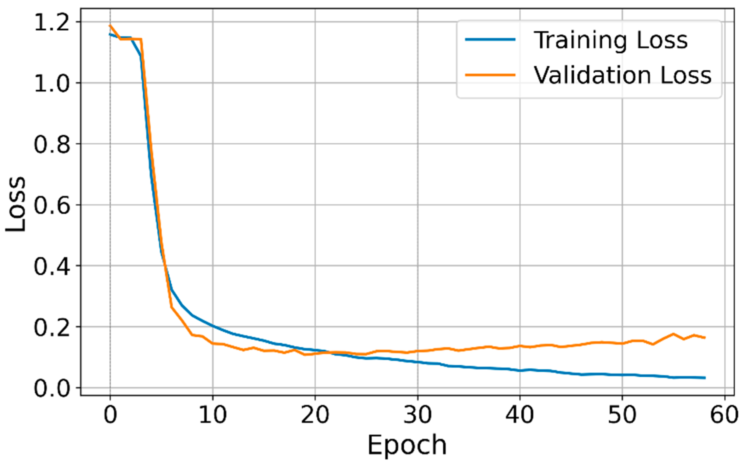
The Hybrid converged well during training, with only mild signs of overfitting. As shown in Figure 2, the training and validation loss decreased steadily and rose slightly near the end, indicating the onset of overfitting. Convergence was otherwise stable, and each epoch required approximately 31.3 s, with a total training time of about 21 min for 40 epochs on an NVIDIA V100 GPU (NVIDIA Corporation, Santa Clara, CA, USA).

3.2. Model Performance (Fixed Threshold, τ = 0.70)

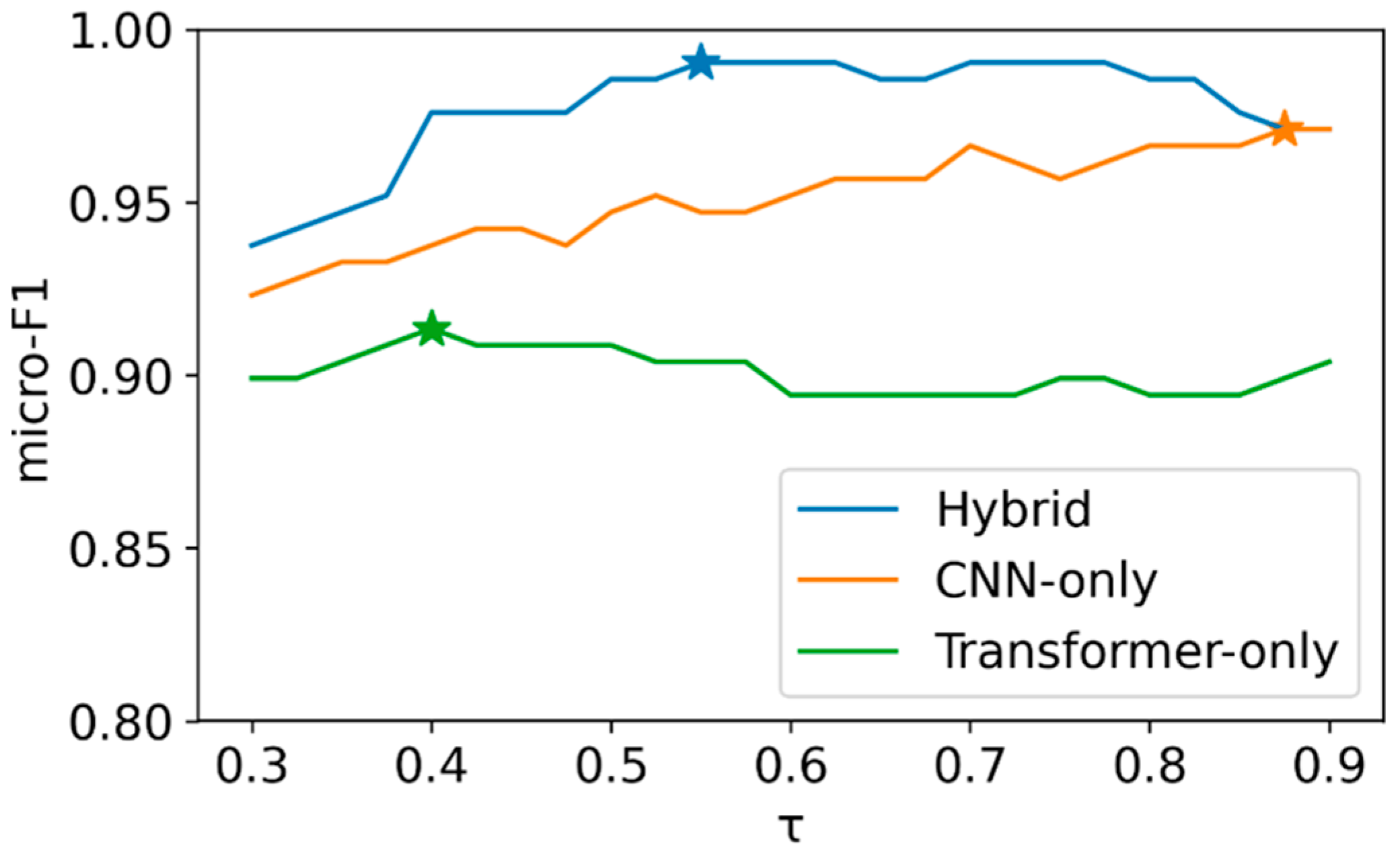
The Hybrid achieved high accuracy on real mixtures, with near-perfect per-label predictions and strong exact-match performance (Table 3). On 16 real test spectra with 13 labels each (208 elements), the Hybrid achieved element-wise accuracy, micro-F1 = 0.990 (206/208), and subset (exact-match) accuracy = 0.875 (14/16). The 95% CI for subset accuracy was [0.617, 0.984]. The Hybrid produces sharp probabilities but only moderate calibration on the REAL set (Brier = 0.0179, ECE ≈ 0.70, 15 bins). Post hoc temperature scaling had a negligible effect (T ≈ 1.0). The model is compact (~0.47 M parameters) and fast (~0.68 ms per spectrum on GPU). A τ-sweep (Figure 3) shows a broad operating plateau and consistent outperformance of the ablations; per-class precision/recall at τ = 0.70 is near-perfect for most ingredients, with a few small-support exceptions (Figure 4). Representative REAL spectra and curated failure/ambiguous cases are provided in Figures S6 and S7. Each spectrum is shown on the analysis ppm grid with per-class probabilities (dashed line at τ = 0.70); the errors largely reflect peak overlap, low SNR/dilution, or baseline/phase imperfections.
The threshold sweeps confirm robustness to the operating-point choice. On the REAL set (Figure 3), the best global thresholds were Hybrid τ* = 0.55 (micro-F1 0.990, subset 0.875, element-wise 0.990), CNN-only τ* = 0.875 (micro-F1 0.971, subset 0.688), and Transformer-only τ* = 0.40 (micro-F1 0.913, subset 0.313). Notably, the preregistered τ = 0.70 matches the Hybrid’s best-τ performance to three decimals, indicating a broad stable operating region.
The model demonstrated strong robustness to outsider components, with per-class thresholds reducing false positives (Table 4). For pure outsiders (spectra containing only simulated non-library peaks), the AUROC (max-probability OOD score) was 0.984. At τ = 0.70, the element-wise false positive rate (FPR) was 0.048 and the any-positive (per-spectrum) FPR was 0.320; per-class thresholds reduced them to 0.032 and 0.215, respectively. For mixed outsiders (known library components plus outsiders), performance on known labels remained strong (micro-F1/precision/recall ≈ 0.84–0.85), while hallucinations decreased with per-class thresholds (element-wise FPR 0.036 vs. 0.048; any-positive 0.219 vs. 0.309).
Trained on simulation and evaluated once on REAL, the PCA + LR and PLS-DA produced near-uninformative probabilities on REAL (concentrated near 0.5). At the Hybrid operating point τ = 0.70, both collapsed to the all-zero decision, giving micro-F1/precision/recall = 0.736 and subset accuracy = 0.00 (Brier ≈ 0.25 and ECE ≈ 0.235). Using the SIM-selected global threshold (τ*) = 0.65 gave identical outcomes. At the default τ = 0.50, performance moved off the trivial rule but remained weak: PCA + LR 0.572 and PLS-DA 0.500 (micro-F1/precision/recall), with subset accuracy = 0.00 for both (Table S1). Because predictions are effectively trivial at τ ≥ 0.6, McNemar’s test is not informative and is omitted; comprehensive descriptive metrics are reported instead. Distributional projections, PCA and UMAP in Figures S4 and S5, respectively, show REAL embedded within the SIM distribution, consistent with strong SIM-to-REAL transfer of the Hybrid and the weakness of linear chemometric baselines.
Ablation experiments confirmed that both CNN and Transformer components are necessary for top performance (Table 2 and Table 5). Across fixed τ = 0.70, best global τ*, and per-class thresholds, Hybrid outperforms both the CNN-only and Transformer-only. At τ = 0.70, the results were CNN-only 0.971/0.688 and Transformer-only 0.913/0.313 (element-wise/subset). With each model’s best τ* (CNN-only 0.875; Transformer-only 0.40), the ordering is unchanged. On GPU (V100), the latencies of CNN-only and Transformer-only were 0.28 ms, and 0.37 ms, respectively (Table 5).
Pairwise statistical tests supported the Hybrid’s significant advantage over the Transformer-only baseline (Table 6). McNemar’s exact test at τ = 0.70 showed the following: Element-wise Hybrid vs. CNN-only: discordant = 7 (b = 1, c = 6), p = 0.125; Hybrid vs. Transformer-only: discordant = 24 (b = 2, c = 22), p = 3.59 × 10⁻⁵; Subset (exact-match) Hybrid vs. CNN-only: discordant = 5 (b = 1, c = 4), p = 0.375; Hybrid vs. Transformer-only: discordant = 8 (b = 0, c = 8), p = 0.00781.

4. Discussion

A single-pass Hybrid delivers high accuracy on real 1H NMR mixtures while simplifying inference. Casting mixture identification as joint multi-label prediction yields element-wise (micro-F1) = 0.990 (206/208) and subset (exact-match) = 0.875 (14/16) on the REAL set—without per-class comparisons or heuristics. In contrast, prior pairwise methods like DeepMID [9] and FlavorFormer for NMR [10], and DeepRaman [14] for Raman, which compare each mixture with each reference via a pseudo-Siamese CNN + Spatial Pyramid Pooling (SPP), require O(C) evaluations per spectrum and emphasize binary per-class detection rather than joint reasoning.
Hybridization explains the gap to CNN-only and Transformer-only baselines: local multiplet fidelity plus global dependency modeling are both needed. The CNN front-end encodes line-shape/multiplet detail and denoises baseline/ripple; the Transformer aggregates long-range evidence (co-occurrence, mutual exclusion) across distant ppm regions. This division of labor matches experience in spectroscopy and hyperspectral imaging, where CNN–Transformer hybrids consistently beat single-family models by uniting local and global cues [15]. Our ablations mirror this as well: at τ = 0.70, the Hybrid reaches 0.990/0.875 vs. 0.966/0.688 (CNN-only) and 0.894/0.375 (Transformer-only). These findings highlight that convolutional feature extraction is essential in NMR analysis and that Transformers are most effective when integrated with a strong CNN foundation [16]. The CNN component also rapidly reduces the spectral length and extracts key local features [17], lowering the computational burden for the Transformer encoder.
McNemar tests show a significant advantage element-wise (p = 3.59 × 10⁻⁵) and at the subset level (p = 0.00781) for Hybrid vs. Transformer-only; differences vs. CNN-only are directionally favorable but not statistically significant (p = 0.125, 0.375), reflecting small N = 16 and subset-level ties. We nonetheless adopt Hybrid as it preserves CNN-only element-wise accuracy while improving exact-match and calibration under shift. The operating point is forgiving, enabling a single global threshold in practice. A τ-sweep reveals a broad plateau: the preregistered τ = 0.70 essentially matches the Hybrid’s best-τ performance (τ* = 0.55) to three decimals. Mean per-class thresholds (τ ≈ 0.723) do not materially change the metrics, favoring one-line deployment.
The calibration accuracy is moderate (ECE ≈ 0.70, 15 bins), despite sharp probabilities (Brier = 0.0179). The higher ECE arises from our element-wise computation on raw per-class probabilities: many true negatives are correct (accuracy ≈ 1), despite having small p (low “confidence”), yet inflating ∣acc−conf∣ at the bin level [18].
Linear chemometric pipelines (PCA + LR/PLS-DA) trained on simulation did not transfer to REAL (probabilities ≈ 0.5; exact-match 0.00), whereas the same simulation enabled strong transfer for the Hybrid CNN–Transformer. This suggests the limitation is primarily the linear low-capacity assumptions of chemometrics under the SIM-to-REAL shift rather than simulator inadequacy.
Multi-label classification naturally handles outsiders better than closed-set “decomposition to ratios” pipelines. Methods that force a spectrum to be expressed as ratios over a fixed library, whether via pairwise pSNN/pSCNN + SPP with per-class aggregation [9,14] or via direct ratio regression with an FCN [19], implicitly assume that the mixture lies within the known library, leaving no “none-of-the-above” option. Outsider peaks are therefore redistributed onto known classes, inflating false positives. By contrast, our single-pass multi-label Hybrid outputs per-class probabilities in one shot and can simply not activate any class when evidence is inconsistent (via a global or per-class threshold, or an abstain rule based on the maximum class probability) [20]. Empirically, this yields strong OOD behavior: for pure outsiders, we observe an AUROC = 0.984 and can reduce the element-wise FPR from ≈0.048 to ≈0.032 and the any-positive FPR from ≈0.320 to ≈0.215 by moving from a single τ to per-class thresholds; for mixed outsiders, the known-label performance remains high (micro-F1/precision/recall ≈ 0.84–0.85), while hallucinations drop with per-class τ. In short, the advantage with outsiders stems not only from using a Transformer but from the multi-label decision paradigm itself, which permits abstention instead of mass-conserving projection onto the library.
Robustness arises from both architectural bias and domain-informed simulation. The Hybrid keeps class probabilities low when spectra lack consistent class-specific motifs (architectural effect), while the simulator teaches the envelope of normal variability (shift/warp, lineshape/phase, baseline/ripple, noise, dilution, polarity, robust normalization), reducing spurious activations on instrument quirks. Unlike works focused on pairwise matching and augmentation (DeepMID/DeepRaman), our study trains only on SIM spectra and evaluates on REAL measurements; the good performance is consistent with broader reports that domain-specific perturbations help generalization in spectral tasks. Adding outlier exposure (synthetic outsiders with a confidence penalty) and an abstain/energy head would further lower any-positive FPR without harming recall.
Compared with DeepMID-style systems, our contribution is a formulation and evaluation shift rather than a mere architectural tweak: single-pass joint multi-label inference with calibration and OOD evaluation, O(1) inference in library size, and a compact footprint (~0.47 M parameters, ~0.68 ms/spectrum GPU, V100). The limitations motivate clear next steps: (i) expand real/external datasets (current N = 16) to narrow CIs, (ii) improve calibration (ECE) with post hoc scaling or small ensembles, and (iii) broaden the 13-class library and acquisition protocols to strengthen external validity. With these extensions, a compact, simulation-trained, and single-pass multi-label model offers a scalable route to accurate deployable NMR mixture decomposition.

5. Conclusions

A compact CNN–Transformer (“Hybrid”) trained entirely on realistically simulated spectra decomposes complex 1H NMR flavor mixtures in a single pass, delivering high accuracy on the REAL set (micro-F1 = 0.990; exact-match = 0.875), strong robustness to outsider peaks, and clear efficiency/accuracy gains over CNN-only and Transformer-only baselines. Pairing domain-informed simulation with joint multi-label prediction effectively bridges the SIM-to-REAL gap and remains resilient to dilution, peak overlap, and common instrumental artifacts. The main limitations are the small real evaluation set (N = 16) and moderate calibration (despite a low Brier), pointing to next steps: expand the reference library, incorporate matrix effects and cross-instrument protocols, and tighten calibration/OOD handling (e.g., class-wise temperature scaling or light ensembling) without altering ranking.

Supplementary Materials

The following supporting information can be downloaded at: https://www.mdpi.com/article/10.3390/app152111458/s1, Figure S1: Representative 1H NMR spectra of the 13 individual flavor components; Figure S2: Representative 1H NMR spectra of the 16 formulated flavor mixtures; Figure S3: Workflow of the data-simulation pipeline; Figure S4: PCA overlap between simulated (SIM) and real (REAL) spectra; Figure S5: UMAP overlap between simulated (SIM) and real (REAL) spectra; Figure S6: REAL spectra with model probabilities (insets; τ = 0.70); Figure S7: Misclassified/ambiguous examples (REAL top row, simulation bottom); Table S1: Chemometric baselines trained on simulated spectra and evaluated once on REAL (N = 16 spectra, 13 labels).

Author Contributions

Conceptualization, J.Z.; methodology, J.Z.; software, J.Z.; validation, J.Z.; formal analysis, J.Z.; data curation, J.Z.; writing—original draft preparation, J.Z.; writing—review and editing, J.Z. and K.K.; visualization, J.Z.; funding acquisition, J.Z. and K.K. All authors have read and agreed to the published version of the manuscript.

Funding

This research was funded by the Research Council of Norway (RCN), grant number Nos. 352849 and 344343.

Institutional Review Board Statement

Not applicable.

Informed Consent Statement

Not applicable.

Data Availability Statement

Reference spectra and real mixture measurements are as described in the cited DeepMID study (Molecules 2023, 28, 7380). Script for data simulation and formal analysis is available at https://github.com/ZJiangsan/Hybrid-CNN-Transformer-for-Multi-Label-H-NMR-Flavor-Decomposition (accessed on 23 October 2025). The repository provides demo_test_real.ipynb, which loads pretrained weights, evaluates the 16 REAL mixtures, reports micro-F1 and subset (exact-match) accuracy, and reproduces relevant figures.

Acknowledgments

We thank the DeepMID study for their open-access spectral data, which served as a foundation for our simulation-based training pipeline.

Conflicts of Interest

The authors declare no conflicts of interest.

Abbreviations

The following abbreviations are used in this manuscript:
1HProton (hydrogen-1)
AUROCArea Under the Receiver Operating Characteristic Curve
BCEBinary Cross Entropy (loss)
BrierBrier Score (mean squared error of probabilistic predictions)
CNNConvolutional Neural Network
CPUCentral Processing Unit
ECEExpected Calibration Error
FPRFalse Positive Rate
F1 (micro-F1)Micro-averaged F1 Score (precision–recall harmonic mean aggregated over all labels)
GPUGraphics Processing Unit
IDIn-Distribution
LRLearning Rate
NMRNuclear Magnetic Resonance
OODOut-of-Distribution
O(1), O(C)Big-O Complexity: constant time; linear in number of classes (C)
ppmParts Per Million (chemical shift axis)
pSCNN/pSNNPseudo-Siamese Convolutional Neural Network/Pseudo-Siamese Neural Network
ROCReceiver Operating Characteristic
SPPSpatial Pyramid Pooling
τDecision threshold applied to class probabilities
TPRTrue Positive Rate (recall)
TransformerSelf-attention–based neural network architecture
SIMSimulated Spectra
“REAL” setThe 16 real 1H NMR mixtures from the DeepMID study (13 candidate components)

References

  1. Li, W.; Sun, K.; Li, D.; Bai, T. Algorithm for Automatic Image Dodging of Unmanned Aerial Vehicle Images Using Two-Dimensional Radiometric Spatial Attributes. J. Appl. Remote Sens. 2016, 10, 36023. [Google Scholar] [CrossRef]
  2. Nagana Gowda, G.A.; Raftery, D. NMR Metabolomics Methods for Investigating Disease. Anal. Chem. 2023, 95, 83–99. [Google Scholar] [CrossRef] [PubMed]
  3. Wishart, D.S. Quantitative Metabolomics Using NMR. TrAC Trends Anal. Chem. 2008, 27, 228–237. [Google Scholar] [CrossRef]
  4. Li, M.; Xu, W.; Su, Y. Solid-State NMR Spectroscopy in Pharmaceutical Sciences. TrAC Trends Anal. Chem. 2021, 135, 116152. [Google Scholar] [CrossRef]
  5. Holzgrabe, U. Quantitative NMR Spectroscopy in Pharmaceutical Applications. Prog. Nucl. Magn. Reson. Spectrosc. 2010, 57, 229–240. [Google Scholar] [CrossRef] [PubMed]
  6. Fraga-Corral, M.; Carpena, M.; Garcia-Oliveira, P.; Pereira, A.G.; Prieto, M.A.; Simal-Gandara, J. Analytical Metabolomics and Applications in Health, Environmental and Food Science. Crit. Rev. Anal. Chem. 2022, 52, 712–734. [Google Scholar] [CrossRef] [PubMed]
  7. Monakhova, Y.B.; Godelmann, R.; Kuballa, T.; Mushtakova, S.P.; Rutledge, D.N. Independent Components Analysis to Increase Efficiency of Discriminant Analysis Methods (FDA and LDA): Application to NMR Fingerprinting of Wine. Talanta 2015, 141, 60–65. [Google Scholar] [CrossRef] [PubMed]
  8. Kruger, N.J.; Troncoso-Ponce, M.A.; Ratcliffe, R.G. 1H NMR Metabolite Fingerprinting and Metabolomic Analysis of Perchloric Acid Extracts from Plant Tissues. Nat. Protoc. 2008, 3, 1001–1012. [Google Scholar] [CrossRef] [PubMed]
  9. Wang, Y.; Wei, W.; Du, W.; Cai, J.; Liao, Y.; Lu, H.; Kong, B.; Zhang, Z. Deep-Learning-Based Mixture Identification for Nuclear Magnetic Resonance Spectroscopy Applied to Plant Flavors. Molecules 2023, 28, 7380. [Google Scholar] [CrossRef] [PubMed]
  10. Wei, W.; Wang, Y.; Liao, Y.; Lu, H.; Cai, J.; Cui, Y.; Ding, S.; Li, Y.; Zhao, Y.; Wang, Z. FlavorFormer: Hybrid Deep Learning for Identifying Compounds in Flavor Mixtures Based on NMR Spectroscopy. Microchem. J. 2025, 218, 115372. [Google Scholar] [CrossRef]
  11. Fidalgo, T.K.S.; Freitas-Fernandes, L.B.; Angeli, R.; Muniz, A.M.S.; Gonsalves, E.; Santos, R.; Nadal, J.; Almeida, F.C.L.; Valente, A.P.; Souza, I.P.R. Salivary Metabolite Signatures of Children with and without Dental Caries Lesions. Metabolomics 2013, 9, 657–666. [Google Scholar] [CrossRef]
  12. Head, T.; Giebelhaus, R.T.; Nam, S.L.; de la Mata, A.P.; Harynuk, J.J.; Shipley, P.R. Discriminating Extra Virgin Olive Oils from Common Edible Oils: Comparable Performance of PLS-DA Models Trained on Low-field and High-field 1H NMR Data. Phytochem. Anal. 2024, 35, 1134–1141. [Google Scholar] [CrossRef]
  13. Pembury Smith, M.Q.R.; Ruxton, G.D. Effective Use of the McNemar Test. Behav. Ecol. Sociobiol. 2020, 74, 133. [Google Scholar] [CrossRef]
  14. Fan, X.; Wang, Y.; Yu, C.; Lv, Y.; Zhang, H.; Yang, Q.; Wen, M.; Lu, H.; Zhang, Z. A Universal and Accurate Method for Easily Identifying Components in Raman Spectroscopy Based on Deep Learning. Anal. Chem. 2023, 95, 4863–4870. [Google Scholar] [CrossRef]
  15. Zhang, P.; Yu, H.; Li, P.; Wang, R. TransHSI: A Hybrid CNN-Transformer Method for Disjoint Sample-Based Hyperspectral Image Classification. Remote Sens. 2023, 15, 5331. [Google Scholar] [CrossRef]
  16. Arkin, E.; Yadikar, N.; Xu, X.; Aysa, A.; Ubul, K. A Survey: Object Detection Methods from CNN to Transformer. Multimed. Tools Appl. 2023, 82, 21353–21383. [Google Scholar] [CrossRef]
  17. Li, Z.; Chen, G.; Zhang, T. A CNN-Transformer Hybrid Approach for Crop Classification Using Multitemporal Multisensor Images. IEEE J. Sel. Top. Appl. Earth Obs. Remote Sens. 2020, 13, 847–858. [Google Scholar] [CrossRef]
  18. Guo, C.; Pleiss, G.; Sun, Y.; Weinberger, K.Q. On Calibration of Modern Neural Networks. In Proceedings of the International Conference on machine Learning, Sydney, Australia, 6–11 August 2017; pp. 1321–1330. [Google Scholar]
  19. Zhao, J.; Kusnierek, K. A Fully Connected Network (FCN) Trained on a Custom Library of Raman Spectra for Simultaneous Identification and Quantification of Components in Multi-Component Mixtures. Coatings 2024, 14, 1225. [Google Scholar] [CrossRef]
  20. Hendrycks, D.; Gimpel, K. A Baseline for Detecting Misclassified and Out-of-Distribution Examples in Neural Networks. arXiv 2016, arXiv:1610.02136. [Google Scholar]
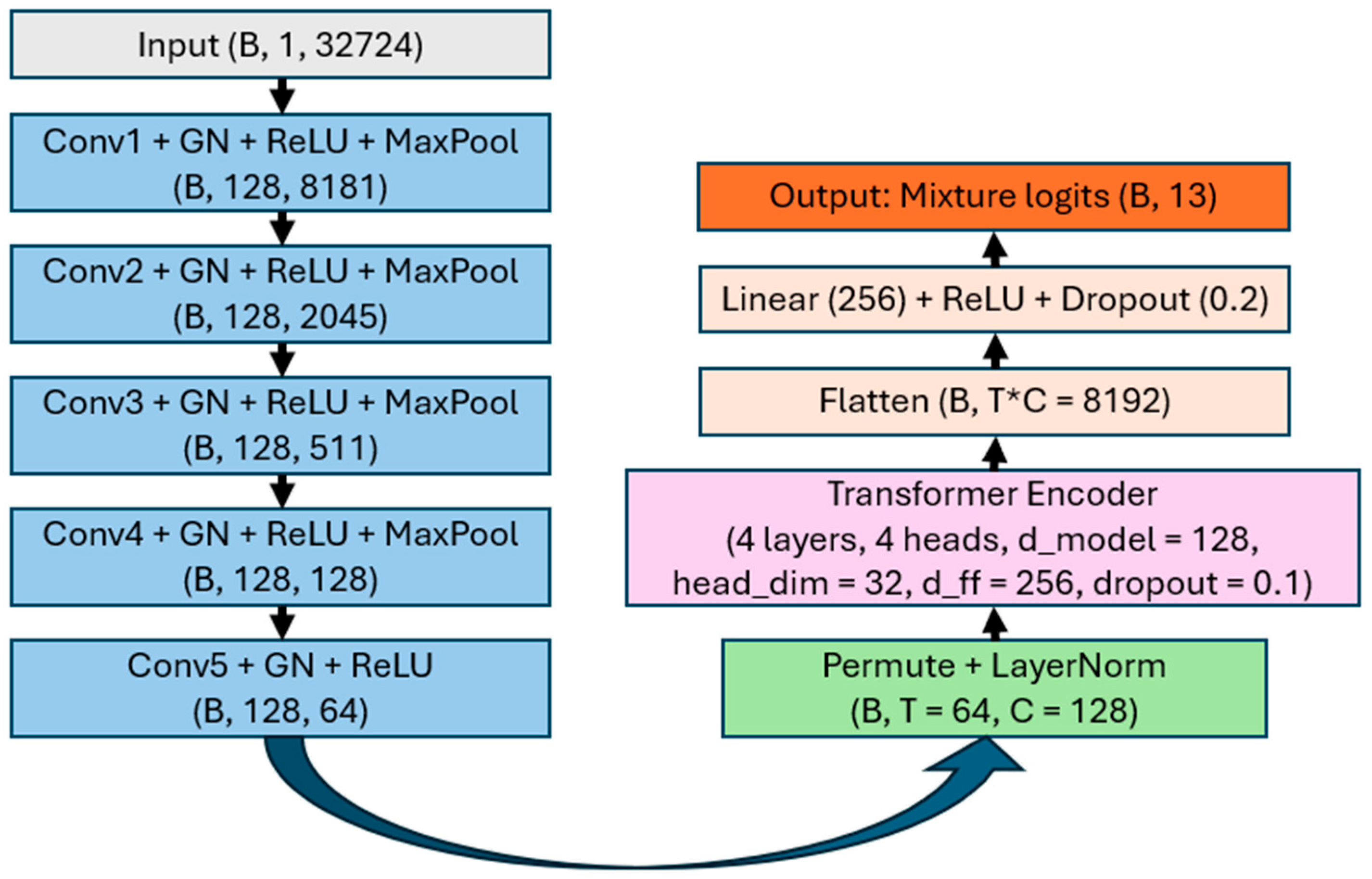
Figure 1. The architecture of Hybrid for NMR spectrum decomposition. Five convolutional layers extract local multiplet features and downsample spectra to 64 × 128 tokens, which the Transformer encoder analyzes before sigmoid classification into 13 flavor components.
Applsci 15 11458 g001
Figure 2. Training and validation loss curves of the Hybrid model using binary cross entropy. Early stopping selects the minimum validation loss; the late uptick indicates mild overfitting.
Applsci 15 11458 g002
Figure 3. Micro-F1 versus decision threshold τ for Hybrid, CNN-only, and Transformer-only models. The five-pointed stars indicate the optimal thresholds yielding the highest micro-F1 scores for each model. Hybrid dominates across decision thresholds (τ), showing a broad operating plateau, confirming robustness to threshold choice.
Applsci 15 11458 g003
Figure 4. Per-class precision and recall at τ = 0.70 on the real NMR mixtures. Most ingredients are predicted almost perfectly; small deviations occur for rarely occurring flavors.
Applsci 15 11458 g004
Table 1. Overview of the 13-component flavor library used for model development.
NameVendor
Alfalfa ExtractionGuangzhou Huafang Tobacco Flavor Co., Ltd., Guangzhou, China
Carob ExtractionGuangzhou Huafang Tobacco Flavor Co., Ltd., Guangzhou, China
Chicory ExtractionGuangzhou Huafang Tobacco Flavor Co., Ltd., Guangzhou, China
Fig ExtractionGuangzhou Huafang Tobacco Flavor Co., Ltd., Guangzhou, China
Galbanum ExtractionGuangzhou Huafang Tobacco Flavor Co., Ltd., Guangzhou, China
Hops ExtractionGuangzhou Huafang Tobacco Flavor Co., Ltd., Guangzhou, China
Plum ExtractionGuangzhou Huafang Tobacco Flavor Co., Ltd., Guangzhou, China
Raisin ExtractionGuangzhou Huafang Tobacco Flavor Co., Ltd., Guangzhou, China
Roman Chamomile Extraction-AGuangzhou Huafang Tobacco Flavor Co., Ltd., Guangzhou, China
Roman Chamomile Extraction-BZhuhai Guanglong Flavor Co., Ltd., Zhuhai, China
Tobacco Maillard ReactantsGuangzhou Huafang Tobacco Flavor Co., Ltd., Guangzhou, China
Valerian Root ExtractionGuangzhou Huafang Tobacco Flavor Co., Ltd., Guangzhou, China
Yunnan Tobacco ExtractionGuangzhou Huafang Tobacco Flavor Co., Ltd., Guangzhou, China
Table 2. Key parameters of the simulated-data generator and augmentations used for training.
BlockParameterSymbolSetting (Range)Rationale
LibraryClasses; lengthC, LC = 13; L = 32,72413 pure references;
full spectrum length
Mixture designComponents per
mixture
K{2, 3, 4, 5, p(K) ∝ (13 choose K)0.8}Stratified over combinatorics
Class priorComponent indicesUniform, no replacementBalanced sampling
RatiosEqual vs. Dirichletp_equal, αp_equal = 0.80;
Dirichlet α = {0.5, 1.0, 2.0}
Match real equal-ratio setting; add variability
AxesShift/warp/stretchΔ, sΔ ∈ [−12, 12]; warp 5–8 knots;
s ∈ [0.985, 1.015] (p = 0.5)
Referencing + drift
DilutionLeveldD ∈ [0.01, 1.00]; scale by (1 − d)Low-SNR realism
LineshapeSmoothing/phaseσ, φΣ ∈ [0.06, 0.20]; φ ~ N(0, 4°)Linewidth + jitter
Baseline and noiseBaseline/ripple/noisea0, a1, a2; A, fQuad baseline; ripple A ∈ [0, 0.006],
f ∈ [1, 3]; white [2 × 10⁻⁴, 6 × 10⁻⁴];
LF λ ∈ [0, 2 × 10⁻⁴]
Instrumental artifacts
PolarityGlobal flipp_flip0.50Polarity invariance
NormalizationRobust scaling80%:/P90|x|; 20%:/max|x|Avoid overfitting to one rule
LabelsPresence/targetsτ_pres, yτ_pres = 0.01; y normalized over
present
Polarity and dilution invariant
DatasetSize/splitNN = 30,000; train/val = 0.8/0.2Deterministic seeds/loaders
Table 3. Performance of Hybrid and ablations on the REAL set.
ModelElem. AccMicro-F1Subset AccECEBrierBest
τ*
Elem. Acc (τ*)Subset Acc (τ*)Per-Class τElem. Acc (τ_c)Subset Acc (τ_c)
Hybrid0.9900.9900.8750.6980.0180.550.9900.8750.7230.9900.875
CNN-only0.9660.9660.6880.6830.0380.8750.9710.6880.7440.9710.688
Transformer-only0.8940.8940.3750.7080.0790.400.9140.3130.7580.8990.375
Table 4. Open-set robustness of the Hybrid to simulated outsider components.
ScenarioThresholding SchemeAUROC (Max-Prob)Any-Pos FPRElem. FPRMicro-F1 (Known)Micro-PMicro-RElem. FPR (Negatives)Any-FP (per Spectrum)
Pure outsidersfixed0.9840.3200.048
per-class0.9840.2150.032
Mixed outsidersfixed0.8430.8430.8430.0480.309
per-class0.8480.8480.8480.0360.219
Table 5. Ablation/effectiveness table with param counts and measured GPU latency.
VariantParams (M)Tokens × DimsBest τ*Micro-F1 (Real)Subset accms/Sample (GPU)
Hybrid~0.4764 × 1280.550.9900.8750.68
CNN-only~0.3764 × 128 (pre-flatten)0.8750.9710.6880.28
Transformer-only~0.4464 × 1280.400.9130.3130.37
Table 6. McNemar’s exact test comparing Hybrid with CNN-only and Transformer-only models on REAL set.
LevelComparisonb (A Wrong/B Right)c (A Right/B Wrong)Discordantp-Value
ElementwiseHybrid vs. CNN-only1670.125
ElementwiseHybrid vs. Transformer-only222243.59 × 10−5
Subset (exact-match)Hybrid vs. CNN-only1450.375
Subset (exact-match)Hybrid vs. Transformer-only0880.00781
Disclaimer/Publisher’s Note: The statements, opinions and data contained in all publications are solely those of the individual author(s) and contributor(s) and not of MDPI and/or the editor(s). MDPI and/or the editor(s) disclaim responsibility for any injury to people or property resulting from any ideas, methods, instructions or products referred to in the content.