Adaptive Graph Neural Network-Based Hybrid Approach for Long-Term Photovoltaic Power Forecasting

Abstract

Photovoltaic power generation prediction is crucial for the effective integration of renewable energy into the grid, real-time grid balancing, and the optimization of energy storage systems. However, PV power generation is highly dependent on environmental factors such as weather conditions. Photovoltaic power generation prediction is crucial for the effective integration of renewable energy into the grid, real-time grid balancing, and the optimization of energy storage systems. However, PV power generation is highly dependent on environmental factors such as weather conditions. Effectively integrating environmental information remains a major challenge for photovoltaic power forecasting. This study proposes a hybrid deep learning model that incorporates an adaptive neural network to capture the latent relationships between PV power generation and environmental variables, thereby enhancing forecasting accuracy. The adaptive graph neural network employs a data-driven directed graph structure, where TCN and variable interaction layers are alternately stacked to better model the spatiotemporal coupling among variables for long-term PV output forecasting. The proposed model was evaluated on three sites located in different regions, with a fixed input length of 96 and output horizons ranging from 96 to 768 steps. Compared with state-of-the-art baselines, the model achieved average improvements of 2.19% and 1.57% in MSE and MAE at a 384-step horizon, and 2.81% and 2.47% at a 768-step horizon, respectively, demonstrating superior performance in long-term PV output forecasting tasks.

1. Introduction

The global demand for energy has continued to rise gradually and significantly in recent years. The excessive exploitation and consumption of fossil fuels has resulted in substantial air pollution and other environmental issues [1]. With the intensifying global energy crisis, renewable energy sources such as photovoltaic (PV) power generation, wind energy, and hydropower have garnered significant worldwide attention for their environmentally friendly attributes such as low-carbon emissions and cleanliness, which contribute to the mitigation of environmental pollution issues [2]. Among these, PV power generation, as one of the most widely adopted renewable energy technologies, plays a crucial role in ensuring the continuous, stable, and economical operation of power systems [3]. According to statistics, the global renewable energy capacity increased by 260 GW in 2020, with solar photovoltaics accounting for nearly half of this expansion [4].

Thee accurate forecasting of PV power output enables smart grids to efficiently manage and integrate solar energy generation [5]. PV power forecasting in smart grids can be practically applied from four perspectives. First, energy management enables grid operators to plan and adjust power supply to reliably meet demand. By accurately predicting renewable energy generation, operators dynamically regulate electricity supply in real-time, reduce the risk of blackouts, and enhance grid reliability. Second, long-term planning for future capacity requirements supports informed investment decisions in grid infrastructure. Third, forecasting assists in energy market operations by helping to set prices and facilitating renewable energy credit trading. Finally, risk management involves identifying potential supply disruptions and taking appropriate measures to minimize their impact [6]. However, PV power production is highly susceptible to weather conditions and other environmental factors, exhibiting inherent intermittency, volatility, and randomness. These characteristics pose considerable challenges to achieving high-precision PV power prediction and smart control.

Numerous researchers have been actively engaged in the study of photovoltaic PV power forecasting. PV power forecasting methods can be generally categorized into physical models, statistical learning methods, and machine learning models [7]. Physical models establish mathematical relationships between PV power output and solar radiation, typically calculated using numerical weather prediction or satellite-derived models [8]. These approaches require detailed considerations such as PV system location, panel tilt angle and orientation as well as weather conditions. However, the effectiveness of physical methods is often constrained by model complexity and computational burden, particularly for high-precision modeling [9]. Statistical methods establish mathematical models by extracting patterns of variation from historical data. Compared with physical models, these approaches are generally more suitable for short-term forecasting [10]. Existing statistics-based time series methods have been applied to capture correlations in PV power curves, including exponential smoothing [11], ARMA [12], ARIMA [13], and SARIMA [14]. Although these methods are computationally efficient, their simple structures limit their ability to model complex nonlinear relationships.

With the rapid advancement of machine learning and deep learning technologies, statistical methods have been gradually supplanted by deep learning approaches. In contrast to traditional methods, deep learning methods exhibit stronger nonlinear modeling capabilities and adaptability. They are better equipped to handle complex time series data [15]. The mainstream methods for PV power prediction can be classified into models based on RNN and CNN. For instance, LSTM and BiLSTM, two improved versions derived from RNN, are employed to extract the inherent temporal relationships within PV sequences [16]. Wang et al. [17] enhanced the LSTM model for PV power prediction by incorporating a frequency domain decomposition method, and this approach demonstrated superior prediction performance. Agga et al. [18] proposed CNN-LSTM and ConvLSTM models to forecast the power generation of PV power plants. The results indicated that both CNN-LSTM and ConvLSTM outperformed the LSTM model. Additionally, TCN, a novel convolutional architecture designed for sequential modeling, has shown excellent performance in PV power generation prediction and has been proven to outperform deep learning models such as CNN and LSTM [19]. Xiang et al. [20] introduced a hybrid model combining TCN and LSTM and found that it was more effective in capturing the complex long-term dependencies of spatial and temporal features compared with the CNN-LSTM model. Previous studies on PV power generation prediction using TCN typically involved constructing models by integrating shallow TCN with LSTM. Nevertheless, shallow TCN might not be able to capture the latent temporal patterns and fine-grained temporal information in PV sequences [21]. Moreover, previous methods often relied on a single neural network to extract the spatial relationships among variables, overlooking the fact that the spatial and temporal relationships in multivariate time series are intertwined.

Different forms of neural networks such as CNN [22], RNN [23], and Transformer [24] were applied in photovoltaic power generation prediction. These neural networks have shown significant advantages in modeling real-world time series data. However, one of the major limitations of the above methods is that they do not model the hidden spatial relationships between time series [25]. The environmental factors of multi-variable PV sequences interact with each other and change over time [26]. Photovoltaic power generation is influenced by environmental factors such as solar irradiance, temperature, humidity, and wind speed.

A graph is a type of data structure that can naturally model complex relationships among a set of entities in real-world scenarios. In practice, many types of data inherently exhibit graph-like properties, such as social networks and e-commerce user–item interactions. In fact, numerous time series are spatiotemporally correlated in nature [27]. For such time series, modeling them in the form of networks or graphs can effectively leverage both the data itself and its spatial dependencies to improve the forecasting accuracy. In recent years, GNNs have emerged as a powerful tool for modeling real-world time series data, capable of capturing complex intervariable and temporal relationships. This approach has gained widespread attention and application in the field of traffic prediction [28] and PV forecasting. Hasnat et al. [29] proposed a graph attention network (GAT)-based solar power forecasting framework constructed according to geographical distances. The framework adapts to prediction horizons ranging from several minutes to multiple days by adjusting individual modules within the architecture. Graph neural networks (GNNs) have been widely employed in forecasting for distributed photovoltaic (PV) power stations, where graph structures are used to represent the relationships among distributed sites. Wang et al. [30] developed a domain-adversarial graph neural network-based method for ultra-short-term distributed PV power forecasting, addressing the challenge of data scarcity that arises in virtual power plants due to newly constructed sites or data-sharing limitations. Wang et al. [31] further proposed a dynamic graph network for ultra-short-term distributed PV power forecasting based on a shape–amplitude loss function. In this approach, dynamic graphical data are used to represent interstation correlations, and a dynamic graph network is constructed as the forecasting model. Lin et al. [32] introduced a novel end-to-end deep learning model for the short-term probabilistic forecasting of regional PV generation. The model employed a directed graph-based dynamic spatial convolutional graph neural network, in which multi-source inputs are used to determine the contribution of one PV station to another. Wang et al. [33] also proposed a domain-adversarial graph neural network approach that utilized a GNN encoder to extract spatial features and capture inter-site spatial correlations, thereby improving ultra-short-term distributed PV forecasting under data-scarce conditions. GNNs have become powerful tools for learning non-Euclidean data representations [34], providing new ideas for modeling real-world time series data and capturing the relationships between different variables in multivariable sequences. Combining GNNs with existing time series frameworks is expected to further improve model performance [25]. Han et al. [35] combined the attention mechanism with an adaptive graph neural network to achieve accurate building energy consumption forecasting and optimize energy structure design. Gao et al. [36] proposed an attention-driven spatiotemporal hybrid model that integrated multi-graph structures and attention-based feature fusion to enhance both single-site and multi-site PV power forecasting performance. This paper proposes a PV power generation prediction model based on adaptive GNN, which takes environmental factors into account and inputs them together with photovoltaic power generation data into the model for prediction. In addition, unlike most existing works that focused on short-term forecasting, this work showed a significant improvement in the long-term forecasting results, which is more important to real-world PV applications. The main contributions of this work are summarized as follows:

(1)

A customized graph neural network (GNN) architecture was designed to model the hidden relationship between photovoltaic power generation and environmental factors. The proposed model is a structure where TCN and MLP layers alternate with graph neural network layers, which is conducive to capturing the coupled spatiotemporal features in the data while paying attention to both the global change patterns and local trends of photovoltaic power generation.

(2)

An adaptive graph neural network was used to learn the latent variable relationships from the data. Compared with related works, using directed graphs in long-span prediction tasks can better model the interrelationships between variables in real scenarios, thereby improving the prediction accuracy of the model.

(3)

The proposed method was applied to the real-world photovoltaic power generation prediction of three photovoltaic power sites. In the prediction tasks of the three stations, the proposed model achieved the highest prediction accuracy at prediction steps of 384 and 768, demonstrating good robustness and significant superiority in capturing the peaks, troughs, and fluctuations in long-term photovoltaic power generation.

2. Methodology

2.1. Problem Formulation

This study addressed a multivariate time series forecasting problem, leveraging PV power generation data and environmental information to predict multi-step PV power output at target sites. Let $x_t\in R^N$ denote the multivariate values at time step t with dimension N, where $x_t\left[i\right]\in =R$ represents the value of the i-th variable at time t. The historical sequence of multivariate observations over p time steps is denoted as $X=\{x_{p-1},x_{p-2},\dots ,x_0\}$, and the target future sequence to be predicted is represented as $Y=\{x_1,x_2,\dots ,x_m$}.

From a graph-based perspective, this work treated each variable in the multivariate time series as a node in a graph. The relationships between variables were characterized by an adjacency matrix. The graph G = (V, E, A) was constructed to model the dependencies among the N multivariate variables, where V is the set of nodes, E is the set of edges (each representing a relationship between two nodes), and $A\in R^{N\times N}$ is the adjacency matrix used to quantitatively describe these relationships. The adjacency matrix is defined as follows:

$$A_{ij}=\left\{\begin{array}{l}1 if(v_i,v_j)\in E and i\ne j\\ 0 else\end{array}\right.$$

(1)

The task of photovoltaic (PV) power forecasting in this study was defined as follows: given a fixed-length lookback window of size T, the goal is to perform the multi-step forecasting of PV power generation over the next L time steps.

$$\left\{x_{T-1},x_{T-2},\dots ,x_0\right\}=\{x_1,x_2,\dots ,x_l\}$$

2.2. Proposed Model

The proposed model in this work is shown in Figure 1 and has a two-stage architecture. In the first stage, an adaptive GNN framework is employed to facilitate interactions among variables. This adaptive GNN can automatically extract relationships between node variables from the data to construct an adjacency matrix. Using the adaptively learned adjacency matrix, the framework integrates PV power generation with other environmental variables. The resulting interactively enhanced time series data are then fed into the forecasting module. The forecasting module employs both continuous and interval sampling strategies to extract both local and global temporal features, enabling multi-horizon predictions of PV power generation.

2.3. GNN Module

This study employed an adaptive GNN [37], which is capable of capturing hidden relationships among variables (Figure 2). The architecture primarily consists of a graph construction layer, graph convolutional layers, and temporal convolutional layers. The graph construction layer was designed to generate an adjacency matrix that represents node-to-node connections and captures latent relationships between variables, thereby providing a foundational graph structure for subsequent graph convolutional operations. The graph convolutional layers and temporal convolutional layers are responsible for capturing spatial and temporal dependencies, respectively, working in concert to model complex real-world spatiotemporal interactions.

The temporal convolutional layer comprises multiple TCNs and adopts an inception-style strategy for selecting convolutional kernel sizes. Outputs from four two-dimensional convolutional filters with different kernel sizes were concatenated to enhance multi-scale feature extraction. In order to align with periodic temporal patterns, a time module incorporating four filters with kernel sizes of 1 × 2, 1 × 3, 1 × 6, and 1 × 7 was used. These filter sizes were chosen to comprehensively cover major cyclical frequencies in the temporal domain.

The graph construction layer generates an initial adjacency matrix via node embedding and further refines it through adaptive learning, thereby capturing hidden relationships among nodes in multivariate time series. This process can be formalized as follows:

$$E_1=Embedding(nodes,\dim )$$

(2)

$$E_2=Embedding(nodes,\dim )$$

(3)

$$M_1=\tanh (\alpha E_1{\theta }_1)$$

(4)

$$M_2=\tanh (\alpha E_1{\theta }_1)$$

(5)

$$A=\mathrm{Re}LU(\tanh (\alpha (M_1{M}_2^T-M_2{M}_1^T)))$$

(6)

$$idx=\arg topk(A)$$

(7)

where $E_1$ and $E_2$ represent randomly initialized node embeddings, which are learnable during training. ${\theta }_1$ and ${\theta }_2$ are model parameters that are also optimized through the training process. $\alpha$ is a hyperparameter, manually set, that controls the saturation rate of the node embeddings.

The graph convolutional layer integrates the information of each node with that of its neighbors by separately processing spatial dependencies using a forward adjacency matrix and a reverse adjacency matrix. The processed representations are then fused. During this integration, changes in any node may dynamically influence the states of other nodes. The procedure for handling both the inflow and outflow of information for each node in the graph convolution module is formulated as follows:

$$\widetilde{D_{ii}}=1+{\displaystyle {\sum }_j{A}_{jj}}$$

(8)

$$\tilde{A}={\tilde{D}}^{-1}(A+I)$$

(9)

$$H^{\left(k\right)}=\beta H_{in}+\left(1-\right)\tilde{A}{H}^{(k-1)}$$

(10)

$$H_{\mathrm{out}}={\displaystyle \sum _{i=0}^K{H}^{(k)}}{W}^{(k)}$$

(11)

2.4. Forecasting Module

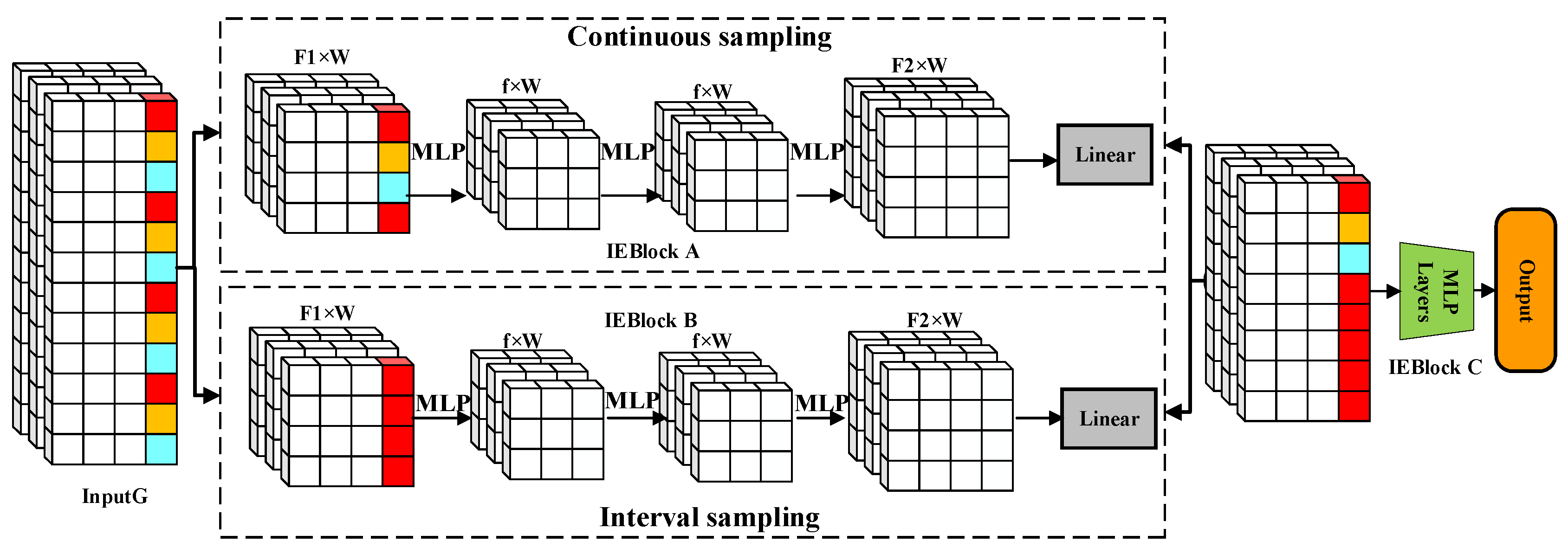
The prediction module employs a lightweight MLP network [38]. This module processes the data transformed by the GNN module through both interval sampling and continuous sampling strategies. Both the sampling and prediction steps utilize an information exchange block (IEBlock) to capture long-term evolutionary trends and fine-grained local variations in the photovoltaic power generation sequence.

The IEBlock operates on a 2D matrix of shape F1×W, where F1 represents the temporal dimension and W denotes the channel dimension. It outputs another matrix of shape F2×W (where F2 is a hyperparameter dependent on the desired output feature dimension), as illustrated in Figure 3. The procedure for processing time series within IEBlock is as follows:

Let $Z={\left(z_{ij}\right)}_{H\times W}$ denote the 2D input matrix processed by each IEBlock. The i-th column is denoted as $z_i={(z_{1i},z_{2i},\dots ,z_{Hi})}^T$, and the j-th row as $z_j={(z_{j1},z_{j2},\dots ,z_{jW})}^T$. For each column, a mapping $R^{F1}=R^f$ (where f < F1) is applied to perform temporal feature extraction. This process is formalized as follows:

$${\mathrm{z}}_{\cdot i}^t=MLP(z_{\cdot i})$$

(12)

Subsequently, column-wise processing is applied to transform $R^W=R^W$, extracting inter-channel features. This procedure is formalized as follows:

$${\mathrm{z}}_{j\cdot }^c=MLP(z_{j\cdot }^t)$$

(13)

Finally, the temporal features undergo an output transformation $R^f=R^{F2}$, where F2 > f. This process is formalized as follows:

$${\mathrm{z}}_{\cdot i}^o=MLP(z_{\cdot i}^c)$$

(14)

3. Datasets and Evaluation Metrics

3.1. Data Description

The data utilized in this study originated from solar power plant datasets collected via a SCADA system by Chen et al. [39]. The power plants are situated in North, Central, and Northwest China, covering diverse climatic and geographic conditions. With installed capacities ranging from 30 MW to 200 MW, the dataset comprises power generation measurements sampled at 15 min intervals over a 24-month period. Three sites were selected from the dataset to evaluate the robustness of the proposed model. The datasets from Site 1 and Site 2 contained outliers and were used to assess the model’s stability. The data were partitioned into training, testing, and validation sets following a 7:2:1 ratio. All three sites shared identical feature sets. The features are detailed in

Table 1. Abbreviations, descriptions, and units of the features.

Abbreviation	Variable Description	Units
TSI	Total solar irradiance	W/m2
DNI	Direct normal irradiance	W/m2
GHI	Global horizontal irradiance	W/m2
AT	Air temperature	°C
AP	Air pressure	hpa
RH	Relative humidity	%
P	Photovoltaic power generation	MW

.

3.2. Evaluation Metrics

To compare the predictive performance among different models, this study employed two evaluation metrics: mean squared error (MSE) and mean absolute error (MAE), defined as follows:

$$MSE={\displaystyle \frac{1}{\mathrm{n}}}{{\displaystyle \sum _{i=1}^n({\widehat{y}}_i-y_i)}}^2$$

(15)

$$MAE={\displaystyle \frac{1}{n}}{\displaystyle \sum _{i=1}^n\left|{\widehat{y}}_i-y_i\right|}$$

(16)

where ${\widehat{y}}_i$ denotes the predicted value generated by the model and $y_i$ represents the corresponding true value.

4. Experiments and Discussion

4.1. Overall Prediction Results

The proposed model was compared against CNN_LSTM, Transformer [40], Autoformer [41], Informer [42], Crossformer [43], MTGNN, LightTS, and GWNet [44]. In all experiments, the input length was fixed at 96 steps, and forecasting horizons were set to 96, 192, 384, and 768 steps, respectively, with a temporal resolution of 15 min.

Table 2. The results of site 1.

	Horizon96		Horizon192		Horizon384		Horizon768
Methods	MSE	MAE	MSE	MAE	MSE	MAE	MSE	MAE
MTGNN	0.817	0.523	1.087	0.633	1.282	0.714	1.472	0.822
Autoformer	1.397	0.812	1.375	0.785	1.578	0.862	1.709	0.903
Transformer	0.917	0.612	1.405	0.766	1.515	0.855	1.606	0.865
LightTS	0.855	0.542	1.086	0.647	1.330	0.729	1.563	0.803
Crossformer	0.767	0.485	1.031	0.603	1.267	0.743	1.502	0.820
Informer	1.356	0.799	1.515	0.877	1.763	0.947	1.953	0.999
CNN_LSTM	1.099	0.664	1.303	0.731	1.418	0.758	1.578	0.801
GWNet	0.994	0.567	1.341	0.691	1.652	0.787	1.827	0.844
Proposed	0.816	0.521	1.058	0.621	1.240	0.703	1.447	0.798

,

Table 3. The results of site 2.

	Horizon96		Horizon192		Horizon384		Horizon768
Methods	MSE	MAE	MSE	MAE	MSE	MAE	MSE	MAE
MTGNN	0.870	0.425	0.853	0.455	0.963	0.505	1.024	0.500
Autoformer	1.374	0.733	1.456	0.734	1.325	0.695	1.285	0.644
Transformer	1.003	0.568	1.116	0.663	1.464	0.755	1.297	0.676
LightTS	0.828	0.417	0.946	0.470	1.025	0.502	1.105	0.522
Crossformer	0.772	0.408	0.893	0.481	0.939	0.537	1.058	0.513
Informer	1.352	0.711	1.372	0.720	1.576	0.821	1.701	0.831
CNN_LSTM	1.041	0.584	1.007	0.570	0.997	0.550	1.151	0.577
GWNet	0.933	0.446	1.040	0.484	1.163	0.547	1.334	0.585
Proposed	0.812	0.416	0.870	0.463	0.926	0.488	0.986	0.473

and

Table 4. The results of site 3.

	Horizon96		Horizon192		Horizon384		Horizon768
Methods	MSE	MAE	MSE	MAE	MSE	MAE	MSE	MAE
MTGNN	0.867	0.634	0.855	0.640	1.063	0.718	1.013	0.696
Autoformer	1.038	0.766	1.244	0.846	1.066	0.792	1.271	0.865
Transformer	0.871	0.663	0.892	0.656	1.119	0.716	1.054	0.714
LightTS	0.904	0.663	1.015	0.709	1.094	0.741	1.156	0.762
Crossformer	0.766	0.478	1.031	0.603	1.326	0.704	1.493	0.776
Informer	1.312	0.834	1.395	0.885	1.676	0.968	1.823	1.037
CNN_LSTM	0.932	0.654	0.988	0.700	1.297	0.787	1.332	0.804
GWNet	0.807	0.605	0.973	0.669	1.169	0.734	1.217	0.749
Proposed	0.771	0.602	0.816	0.635	1.032	0.702	0.985	0.687

list the MSE and MAE values obtained by different methods across different horizons at the three sites. Bold denotes the best results and underline denotes the second-best results, respectively. As shown, the proposed model achieved favorable predictive performance across all forecasting horizons at the three sites. It demonstrated particularly superior results at the 384 and 768-step horizons, outperforming all other compared models. Crossformer consistently outperformed other models at the 96 and 192-step horizons, indicating its strength in short-term forecasting. Among all Transformer variants, Crossformer exhibited superior performance at every horizon, which can be attributed to its dedicated module for capturing temporal patterns and inter-variable correlations, thereby improving the prediction accuracy. In contrast, GWNet overly emphasized the extraction of spatial information while failing to adequately incorporate crucial temporal patterns, resulting in relatively lower accuracy. These results demonstrate that models simultaneously capturing both spatial and temporal dimensions consistently outperformed those modeling only a single dimension. In general, the proposed model ranked among the top two performers across all models at 96 and 192-step horizons and achieved the best forecasting results at 384 and 768 steps, demonstrating strong robustness. Compared with the strongest baseline model, it yielded average improvements in MSE and MAE of 2.19% and 1.57% at the 384-step horizon, and 2.81% and 2.47% at the 768-step horizon, respectively, and the relatively lower short-term forecasting performance compared with Crossformer may be attributed to the two-stage attention module in Crossformer, where the multi-head attention mechanism enables finer modeling of short temporal dependencies. In contrast, the proposed model focuses more on leveraging multidimensional variable information, which is more advantageous for capturing long-term temporal dependencies and thus enhances long-horizon forecasting performance.

To evaluate the stability of the model, we conducted 15 repeated runs without fixing the random seed on datasets from three different sites, with prediction horizons ranging from 96 to 768 steps. MSE and MAE were statistically aggregated, and 95% confidence intervals were calculated for the model’s performance at each site. The resulting confidence intervals are presented in

Table 5. Statistical analysis of model performance variability.

Horizon	96		192		384		768
Metric	MSE	MAE	MSE	MAE	MSE	MAE	MSE	MAE
1	0.814 ± 0.010	0.522 ± 0.006	1.240 ± 0.022	0.703 ± 0.010	1.447 ± 0.027	0.798 ± 0.015	1.240 ± 0.022	0.703 ± 0.010
2	0.812 ± 0.026	0.419 ± 0.011	0.926 ± 0.012	0.488 ± 0.011	0.999 ± 0.013	0.487 ± 0.012	0.926 ± 0.012	0.488 ± 0.011
3	0.771 ± 0.025	0.602 ± 0.009	1.032 ± 0.013	0.704 ± 0.005	0.985 ± 0.020	0.688 ± 0.006	1.032 ± 0.013	0.704 ± 0.005

, the model exhibited relatively small overall errors across multiple prediction horizons and all three site datasets, demonstrating satisfactory stability.

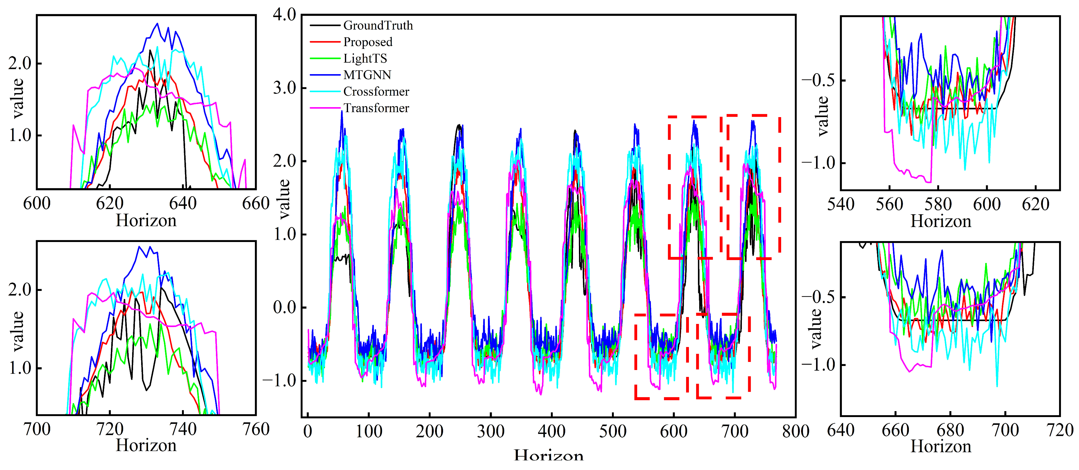
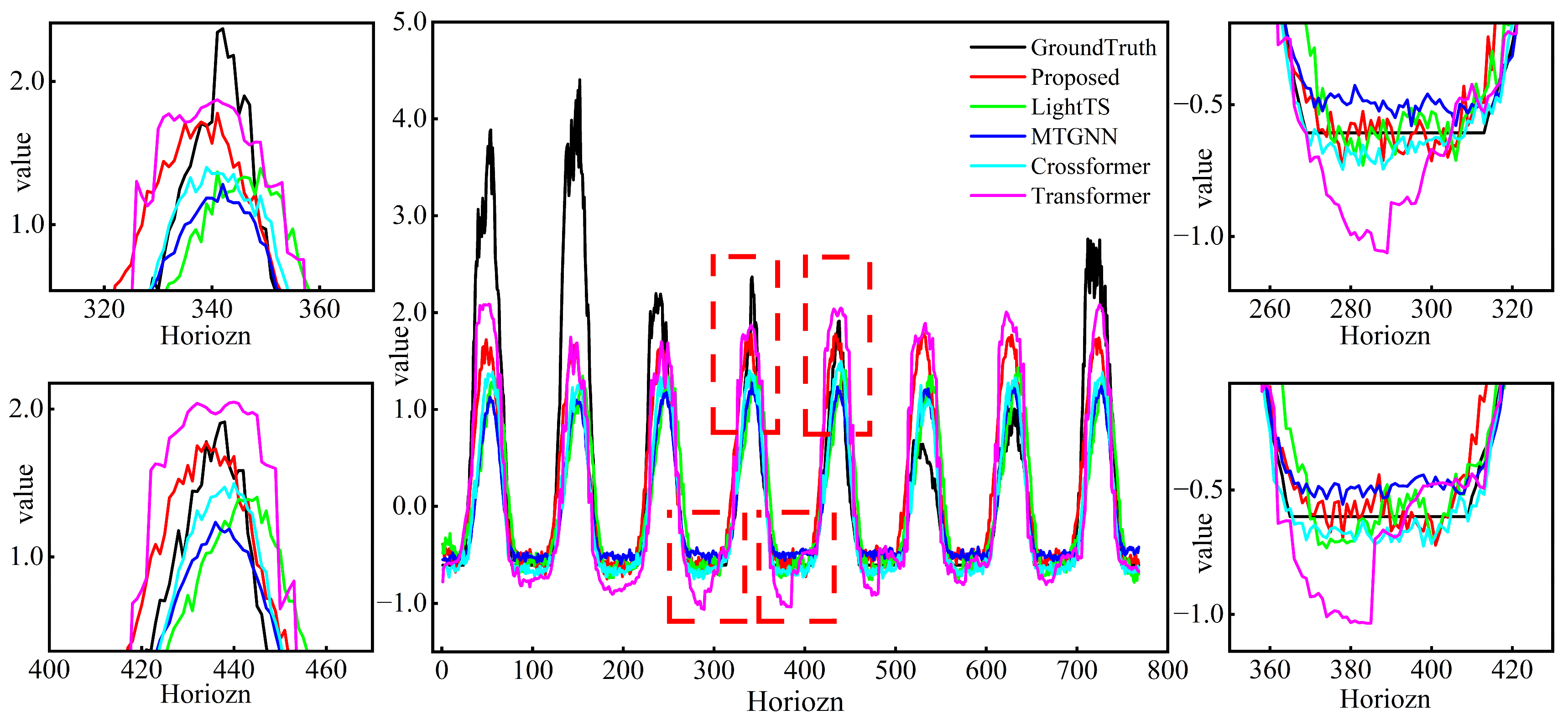
As indicated by the above results, the proposed model demonstrated strong performance in long-term forecasting tasks. We visualized the predicted and true PV power curves for the forecasting horizon of 768 steps. The top five baseline models, along with the proposed model, are compared in Figure 4, Figure 5 and Figure 6. While all models showed comparable capability in capturing the overall trends in power generation, the proposed model exhibited notably superior performance in identifying the peaks, troughs, and fluctuations of the PV power output. Compared with the baseline models, its predictions during periods of power variation aligned more closely with the true values, indicating s higher accuracy in both trend capture and fine-grained variation modeling. These characteristics highlight the model’s strong adaptability and high predictive accuracy when handling complex and dynamically changing long-term time series data.

4.2. Effect of the Correlation Coefficient k on Forecasting Accuracy

As shown in Equation (7), the correlation coefficient k determines the number of relevant variables selected for the proposed model. To investigate the impact of the number of input variables on model performance, we evaluated the model on the dataset from site 3 using correlation coefficient values ranging from 1 to 7. The results are presented in

Table 6. Prediction results with different numbers of input variables.

k	Horizon96		Horizon192		Horizon384		Horizon768
	MSE	MAE	MSE	MAE	MSE	MAE	MSE	MAE
1	0.745	0.594	0.827	0.635	1.047	0.711	1.053	0.704
2	0.744	0.592	0.808	0.628	1.045	0.714	1.013	0.694
3	0.735	0.592	0.807	0.635	1.061	0.716	0.992	0.688
4	0.771	0.602	0.800	0.630	1.035	0.706	0.985	0.687
5	0.778	0.607	0.825	0.640	1.061	0.718	1.002	0.693
6	0.779	0.606	0.833	0.638	1.062	0.718	1.028	0.699
7	0.820	0.627	0.861	0.653	1.068	0.720	1.039	0.703

. The model achieved the best overall performance across all prediction horizons when k = 4, particularly for longer forecasting horizons of 384 and 768 steps. An excessive number of input variables introduced noise and interfered with the model’s ability to extract salient features, thereby reducing the predictive accuracy. Conversely, too few variables provided insufficient information, also leading to performance degradation. For shorter forecasting horizons, smaller values of k yielded better results. This indicates that in short-term prediction tasks, a larger number of correlated variables may distract the model from capturing essential temporal patterns, resulting in decreased accuracy.

4.3. Impact of the Adjacency Matrix

To evaluate the impact of graph on prediction accuracy, we conducted experiments on the dataset from site 3, comparing three configurations: directed graph, undirected graph, and no graph structure. The model was tested across forecasting horizons ranging from 96 to 768 steps. Results are presented in

Table 7. Prediction results using different adjacency matrices.

Type	Horizon96		Horizon192		Horizon384		Horizon768
	MSE	MAE	MSE	MAE	MSE	MAE	MSE	MAE
Direct	0.771	0.602	0.816	0.635	1.032	0.704	0.985	0.687
Undirect	0.758	0.599	0.813	0.634	1.039	0.711	0.996	0.691
None	0.753	0.597	0.827	0.642	1.082	0.726	1.043	0.701

. As the prediction horizon increased, the proposed model using the directed graph demonstrated progressively better performance, followed by the undirected graph configuration. This result indicates that the undirected graphs are inadequate for modeling complex variable relationships in longer-term forecasting tasks. In longer-horizon forecasting, the underlying relationships between variables are likely unidirectional, for instance, environmental factors such as weather conditions affect PV power generation, but the PV output does not influence environmental variables, while the directed graph effectively captures such directional dependencies, thereby enhancing the prediction accuracy. Compared with using an undirected graph, the proposed model with a directed graph improved the MSE and MAE by 0.67% and 0.99% at the 384-step horizon and 1.12% and 0.58% at the 768-step horizon, respectively.

4.4. Computational Efficiency Analysis

The computational efficiency and resource consumption of the model directly influence the real-time scheduling speed and deployment of photovoltaic (PV) systems, serving as critical factors for maintaining stable and continuous power output. In this section, a comprehensive evaluation of the model’s computational efficiency and resource utilization was conducted. The experiments employed the torchinfo.sum function to report each model’s architectural statistics including the number of parameters (Param), computational complexity (MACs), memory consumption (Memory), and iteration time per training step (Train-time); the results are presented in

Table 8. Computational efficiency comparison of different methods.

Method	Params	Memory (MB)	MACs (M)	Train-Time (s/iter)
LightTS	83,930	0.320167542	0.090806	0.0226
CNN_LSTM	814,144	3.105712891	14.731904	0.0211
Transformer	864,135	3.296413422	269860.2787	0.4286
Informer	901,191	3.437770844	256598.0943	0.1056
GWNet	1,404,224	5.098876953	277.673152	0.2300
MTGNN	1,521,568	5.780517578	64.460928	0.0589
Crossformer	3,027,428	11.37586975	71.13578	0.1989
Autoformer	35,879,197	7.774822235	75.135751	0.5964
Proposed	1,520,141	5.769996643	63.944918	0.0650
RANK(Proposed)	6	6	3	4

.

As shown in Table 8, the proposed model exhibited relatively larger parameter counts and memory consumption; however, its computational complexity (MACs) and iteration time per training step were comparatively small, ranking just after the lightweight CNN_LSTM and LightTS models. In conjunction with Table 2, it can be observed that although the proposed model sacrificed a certain amount of training time and computational resources, it achieved a substantial improvement in forecasting performance compared with the baseline models. This moderate increase in computational cost, accompanied by a significant enhancement in predictive accuracy, is therefore considered worthwhile.

5. Conclusions

This study presented a long-term photovoltaic (PV) power forecasting model based on customized graph neural networks (GNNs) designed to capture complex spatiotemporal dependencies among multiple variables and to leverage environmental information for enhanced predictive accuracy. The model’s performance was evaluated using MSE and MAE across datasets from three PV power sites. The main experiments and findings are as follows:

(1)

Superior accuracy and robustness: Compared with baseline models, the proposed model achieved the highest accuracy and demonstrated stronger robustness in forecasting horizons of 384 and 768 steps. It improved the MSE and MAE by an average of 2.19% and 1.57% at the 384-step horizon, and 2.81% and 2.47% at the 768-step horizon, respectively, relative to the best-performing baseline. Furthermore, models that captured hidden inter-variable relationships consistently outperformed those focusing solely on temporal patterns or spatial relationships.

(2)

Enhanced long-term predictive capability: To more intuitively demonstrate the model’s predictive performance in long-term photovoltaic (PV) power forecasting, the predicted and true power curves for the 76-step horizon were visualized. The proposed model showed significant advantages in capturing the peak, trough, and fluctuation patterns compared with all baseline models, achieving superior fitting performance.

(3)

Impact of correlation coefficient k: The correlation coefficient k determines the number of relevant variables used for prediction, and an optimal value of k exists. The model achieved its best performance when k = 4, particularly for longer forecasting horizons of 384 and 768 steps. An excessive number of relevant variables introduced informational noise, while too few variables led to the insufficient utilization of contextual information. Both extremes resulted in decreased prediction accuracy

(4)

Impact of correlation coefficient k: The type of graph structure also notably affects the forecasting performance. Incorporating graph information improved the accuracy in longer-horizon predictions. Compared with using an undirected graph, the proposed model with a directed graph achieved the best results at 384 and 768 steps, improving the MSE and MAE by 0.67% and 0.99% at the 384-step horizon and 1.12% and 0.58% at the 768-step horizon, respectively.

The proposed GNN-based framework integrates environmental information to address the challenge of accuracy degradation in long-term PV power forecasting, demonstrating strong robustness, adaptability, and scalability in complex and dynamic environments.

Despite the promising performance of the proposed model, certain limitations remain. In particular, the adjacency matrix employed by the adaptive graph neural network is dynamic and may lack sufficient stability, limiting its ability to fully capture and explain the relationships between PV power generation and the surrounding environmental factors. In future work, we will further explore the interpretability of graph-based models. These efforts aim to facilitate optimal PV installation planning by comprehensively incorporating environmental information, thereby maximizing the power generation efficiency.

References

1. Mansoor, M.; Mirza, A.F.; Ling, Q.; Javed, M.Y. Novel Grass Hopper optimization based MPPT of PV systems for complex partial shading conditions. Sol. Energy 2020, 198, 499–518. [Google Scholar] [CrossRef]
2. Lin, W.; Zhang, B.; Li, H.; Lu, R. Multi-step prediction of photovoltaic power based on two-stage decomposition and BILSTM. Neurocomputing 2022, 504, 56–67. [Google Scholar] [CrossRef]
3. Achariyaviriya, W.; Suttakul, P.; Phuphisith, S.; Mona, Y.; Wanison, R.; Phermkorn, P. Potential reductions of CO2 emissions from the transition to electric vehicles: Thailand’s scenarios towards 2030. Energy Rep. 2023, 9, 124–130. [Google Scholar] [CrossRef]
4. Kaldellis, J.K.; Kavadias, K.A. Cost-benefit analysis of remote hybrid wind-diesel power stations: Case study Aegean Sea islands. Energy Policy 2007, 35, 1525–1538. [Google Scholar] [CrossRef]
5. Wang, F.; Zhang, Z.; Liu, C.; Yu, Y.; Pang, S.; Duić, N.; Shafie-Khah, M.; Catalão, J.P. Generative adversarial networks and convolutional neural networks based weather classification model for day ahead short-term photovoltaic power forecasting. Energy Convers. Manag. 2019, 181, 443–462. [Google Scholar] [CrossRef]
6. Abou Houran, M.; Bukhari, S.M.S.; Zafar, M.H.; Mansoor, M.; Chen, W. COA-CNN-LSTM: Coati optimization algorithm-based hybrid deep learning model for PV/wind power forecasting in smart grid applications. Appl. Energy 2023, 349, 121638. [Google Scholar] [CrossRef]
7. Das, U.K.; Tey, K.S.; Seyedmahmoudian, M.; Mekhilef, S.; Idris, M.Y.I.; Van Deventer, W.; Horan, B.; Stojcevski, A. Forecasting of photovoltaic power generation and model optimization: A review. Renew. Sustain. Energy Rev. 2018, 81, 912–928. [Google Scholar] [CrossRef]
8. Mayer, M.J.; Gróf, G. Extensive comparison of physical models for photovoltaic power forecasting. Appl. Energy 2021, 283, 116239. [Google Scholar] [CrossRef]
9. Ahmed, R.; Sreeram, V.; Mishra, Y.; Arif, M.D. A review and evaluation of the state-of-the-art in PV solar power forecasting: Techniques and optimization. Renew. Sustain. Energy Rev. 2020, 124, 109792. [Google Scholar] [CrossRef]
10. Fan, S.; Geng, H.; Zhang, H.; Yang, J.; Hiroichi, K. Photovoltaic power forecasting model employing epoch-dependent adaptive loss weighting and data assimilation. Sol. Energy 2025, 290, 113351. [Google Scholar] [CrossRef]
11. Tratar, L.F.; Strmčnik, E. The comparison of Holt–Winters method and Multiple regression method: A case study. Energy 2016, 109, 266–276. [Google Scholar] [CrossRef]
12. Chu, Y.; Urquhart, B.; Gohari, S.M.; Pedro, H.T.; Kleissl, J.; Coimbra, C.F. Short-term reforecasting of power output from a 48 MWe solar PV plant. Sol. Energy 2015, 112, 68–77. [Google Scholar] [CrossRef]
13. Bouzerdoum, M.; Mellit, A.; Pavan, A.M. A hybrid model (SARIMA–SVM) for short-term power forecasting of a small-scale grid-connected photovoltaic plant. Sol. Energy 2013, 98, 226–235. [Google Scholar] [CrossRef]
14. Kushwaha, V.; Pindoriya, N.M. Very short-term solar PV generation forecast using SARIMA model: A case study. In Proceedings of the 2017 7th International Conference on Power Systems (ICPS), Pune, India, 21–23 December 2017; IEEE: New York, NY, USA, 2017; pp. 430–435. [Google Scholar]
15. Wang, F.; Zhen, Z.; Mi, Z.; Sun, H.; Su, S.; Yang, G. Solar irradiance feature extraction and support vector machines based weather status pattern recognition model for short-term photovoltaic power forecasting. Energy Build. 2015, 86, 427–438. [Google Scholar] [CrossRef]
16. Huang, X.; Li, Q.; Tai, Y.; Chen, Z.; Liu, J.; Shi, J.; Liu, W. Time series forecasting for hourly photovoltaic power using conditional generative adversarial network and Bi-LSTM. Energy 2022, 246, 123403. [Google Scholar] [CrossRef]
17. Wang, L.; Mao, M.; Xie, J.; Liao, Z.; Zhang, H.; Li, H. Accurate solar PV power prediction interval method based on frequency-domain decomposition and LSTM model. Energy 2023, 262, 125592. [Google Scholar] [CrossRef]
18. Agga, A.; Abbou, A.; Labbadi, M.; El Houm, Y. Short-term self consumption PV plant power production forecasts based on hybrid CNN-LSTM, ConvLSTM models. Renew. Energy 2021, 177, 101–112. [Google Scholar] [CrossRef]
19. Lea, C.; Vidal, R.; Reiter, A.; Hager, G.D. Temporal convolutional networks: A unified approach to action segmentation. In Proceedings of the European Conference on Computer Vision, Amsterdam, The Netherlands, 11–14 October 2016; Springer International Publishing: Cham, Switzerland, 2016; pp. 47–54. [Google Scholar]
20. Xiang, L.; Liu, J.; Yang, X.; Hu, A.; Su, H. Ultra-short term wind power prediction applying a novel model named SATCN-LSTM. Energy Convers. Manag. 2022, 252, 115036. [Google Scholar] [CrossRef]
21. Krizhevsky, A.; Sutskever, I.; Hinton, G.E. ImageNet classification with deep convolutional neural networks. Commun. ACM 2017, 60, 84–90. [Google Scholar] [CrossRef]
22. Zhao, B.; Lu, H.; Chen, S.; Liu, J.; Wu, D. Convolutional neural networks for time series classification. J. Syst. Eng. Electron. 2017, 28, 162–169. [Google Scholar] [CrossRef]
23. Connor, J.T.; Martin, R.D.; Atlas, L.E. Recurrent neural networks and robust time series prediction. IEEE Trans. Neural Netw. 1994, 5, 240–254. [Google Scholar] [CrossRef]
24. Wen, Q.; Zhou, T.; Zhang, C.; Chen, W.; Ma, Z.; Yan, J.; Sun, L. Transformers in time series: A survey. In Proceedings of the Thirty-Second International Joint Conference on Artificial Intelligence, Macao, 19–25 August 2023; pp. 6778–6786. [Google Scholar]
25. Jin, G.; Liang, Y.; Fang, Y.; Shao, Z.; Huang, J.; Zhang, J.; Zheng, Y. Spatio-temporal graph neural networks for predictive learning in urban computing: A survey. IEEE Trans. Knowl. Data Eng. 2023, 36, 5388–5408. [Google Scholar] [CrossRef]
26. Qin, Y.; Song, D.; Chen, H.; Cheng, W.; Jiang, G.; Cottrell, G. A dual-stage attention-based recurrent neural network for time series prediction. arXiv 2017, arXiv:1704.02971. [Google Scholar]
27. Wang, S.; Cao, J.; Philip, S.Y. Deep learning for spatio-temporal data mining: A survey. IEEE Trans. Knowl. Data Eng. 2020, 34, 3681–3700. [Google Scholar] [CrossRef]
28. Zhang, J.; Wang, F.Y.; Wang, K.; Lin, W.H.; Xu, X.; Chen, C. Data-driven intelligent transportation systems: A survey. IEEE Trans. Intell. Transp. Syst. 2011, 12, 1624–1639. [Google Scholar] [CrossRef]
29. Hasnat, M.A.; Asadi, S.; Alemazkoor, N. A graph attention network framework for generalized-horizon multi-plant solar power generation forecasting using heterogeneous data. Renew. Energy 2025, 243, 122520. [Google Scholar] [CrossRef]
30. Wang, Y.; Fu, W.; Wang, J.; Zhen, Z.; Wang, F. Ultra-short-term distributed PV power forecasting for virtual power plant considering data-scarce scenarios. Appl. Energy 2024, 373, 123890. [Google Scholar] [CrossRef]
31. Wang, Y.; Zhao, Z.; Wang, F.; Sun, S.; Cheng, Y.; Yu, J. A Distributed PV Ultra-short-term Power Deterministic and Probabilistic Forecasting Based on Dynamic Graph Network with Shape-amplitude Criteria. IEEE Trans. Ind. Appl. 2025; in press. [Google Scholar] [CrossRef]
32. Lin, F.; Zhang, Y.; Zhao, H.; Huo, W.; Wang, J. Short-term Probabilistic Forecasting for Regional PV Power based on Convolutional Graph Neural Network and Parameter Transferring. IEEE Trans. Power Syst. 2024, 40, 2724–2736. [Google Scholar] [CrossRef]
33. Wang, Y.; Dai, H.; Zhen, Z.; Wang, F.; Wang, J.; Lu, L. Domain Adversarial Graph Neural Network based Regional Distributed PV Ultra-Short-term Power Forecasting Considering Data-Scarce Scenarios. In Proceedings of the 2024 IEEE Power Energy Society General Meeting (PESGM), Seattle, WA, USA, 21–25 July 2024; IEEE: New York, NY, USA, 2024; pp. 1–5. [Google Scholar]
34. Yang, M.; Zhou, M.; Kalander, M.; Huang, Z.; King, I. Discrete-time temporal network embedding via implicit hierarchical learning in hyperbolic space. In Proceedings of the 27th ACM SIGKDD Conference on Knowledge Discovery Data Mining, Singapore, 14–18 August 2021; pp. 1975–1985. [Google Scholar]
35. Han, Y.; Hao, Y.; Feng, M.; Chen, K.; Xing, R.; Liu, Y.; Lin, X.; Ma, B.; Fan, J.; Geng, Z. Novel STAttention GraphWaveNet model for residential household appliance prediction and energy structure optimization. Energy 2024, 307, 132582. [Google Scholar] [CrossRef]
36. Gao, Y.; Liang, L.; Su, T.; Pan, M. An embedded spatiotemporal hybrid model integrating multi-graphs and attention-driven fusion for single-and multi-site photovoltaic power forecasting. Energy Convers. Manag. 2025, 336, 119897. [Google Scholar] [CrossRef]
37. Wu, Z.; Pan, S.; Long, G.; Jiang, J.; Chang, X.; Zhang, C. Connecting the dots: Multivariate time series forecasting with graph neural networks. In Proceedings of the 26th ACM SIGKDD International Conference on Knowledge Discovery Data Mining, Virtual, 23–27 August 2020; pp. 753–763. [Google Scholar]
38. Zhang, T.; Zhang, Y.; Cao, W.; Bian, J.; Yi, X.; Zheng, S.; Li, J. Less is more: Fast multivariate time series forecasting with light sampling-oriented mlp structures. arXiv 2022, arXiv:2207.01186. [Google Scholar] [CrossRef]
39. Chen, Y.; Xu, J. Solar and wind power data from the Chinese state grid renewable energy generation forecasting competition. Sci. Data 2022, 9, 577. [Google Scholar] [CrossRef] [PubMed]
40. Vaswani, A.; Shazeer, N.; Parmar, N.; Uszkoreit, J.; Jones, L.; Gomez, A.N.; Kaiser, Ł.; Polosukhin, I. Attention is all you need. Adv. Neural Inf. Process. Syst. 2017, 30. [Google Scholar]
41. Wu, H.; Xu, J.; Wang, J.; Long, M. Autoformer: Decomposition transformers with auto-correlation for long-term series forecasting. Adv. Neural Inf. Process. Syst. 2021, 34, 22419–22430. [Google Scholar]
42. Zhou, H.; Zhang, S.; Peng, J.; Zhang, S.; Li, J.; Xiong, H.; Zhang, W. Informer: Beyond efficient transformer for long sequence time-series forecasting. In Proceedings of the AAAI Conference on Artificial Intelligence, Virtual, 19–21 May 2021; Volume 35, No. 12. pp. 11106–11115. [Google Scholar]
43. Zhang, Y.; Yan, J. Crossformer: Transformer utilizing cross-dimension dependency for multivariate time series forecasting. In Proceedings of the Eleventh International Conference on Learning Representations, Kigali, Rwanda, 1–5 May 2023. [Google Scholar]
44. Wu, Z.; Pan, S.; Long, G.; Jiang, J.; Zhang, C. Graph wavenet for deep spatial-temporal graph modeling. arXiv 2019, arXiv:1906.00121. [Google Scholar]
Figure 1. Proposed model.
Applsci 15 11452 g001
Figure 2. GNN module.
Applsci 15 11452 g002
Figure 3. Forecasting module.
Applsci 15 11452 g003
Figure 4. Prediction curves of site 1.
Applsci 15 11452 g004
Figure 5. Prediction curves of site 2.
Applsci 15 11452 g005
Figure 6. Prediction curves of site 3.
Applsci 15 11452 g006