Article

Adaptive MEC–RBF Neural Network-Based Deflection Prediction for Prestressed Concrete Continuous Rigid Frame Bridges During Construction

1
School of Transportation Science and Engineering, Harbin Institute of Technology, Harbin 150090, China
2
The First Company of China Eighth Engineering Division Ltd., Jinan 250014, China
*
Author to whom correspondence should be addressed.
Appl. Sci. 2025, 15(21), 11326; https://doi.org/10.3390/app152111326
Submission received: 30 August 2025 / Revised: 15 October 2025 / Accepted: 20 October 2025 / Published: 22 October 2025
(This article belongs to the Special Issue Advances in Bridge Design and Structural Performance: 2nd Edition)

Abstract

A deflection prediction approach based on an adaptive MEC–RBF neural network was developed in this study. By dynamically optimizing the centres, widths, and weights of the RBF network, the proposed method substantially increases the prediction accuracy, and it achieves an R2 of 0.9789 and an RMSE of 1.4978 on the training dataset. It effectively resolves the stability challenges that are associated with nonlinear construction conditions in traditional models. An orthogonal experimental design analysis revealed that the girder block length and the cantilever-to-span length ratio (d/L) were the most influential factors that affected deflection, whereas the effects of uniformly distributed loads and temperature were negligible, thereby providing a sound basis for parameter simplification. The application of the model to the Hannan Yangtze River Bridge yielded a maximum discrepancy of only 5.56 mm (17.7% error rate) between the predicted and measured values, thus demonstrating its practical engineering reliability. By innovatively integrating intelligent optimization techniques with neural networks, this approach overcomes the limitations in terms of real-time responsiveness and long-term stability of conventional methods and offers an efficient and reliable technical tool for the control of large-scale bridge construction.

1. Introduction

In the global infrastructure construction sector, bridge engineering plays a crucial role as both a vital link that connects regional economies and an important indicator of a nation’s civil engineering capabilities [1,2]. With sustained global economic development and accelerated urbanization, increasingly sophisticated demands have been placed on bridge span lengths, design, and construction technologies [3,4]. In particular, under complex geological and hydrological conditions, the demand for long-span bridges continues to increase annually. Owing to their excellent structural performance and adaptability, prestressed concrete continuous rigid frame bridges have become a mainstream choice in modern bridge engineering [5]. In China, bridge construction has achieved globally recognized successes and has resulted in numerous internationally influential bridge projects [6,7]. These successes are attributable to the nation’s strong emphasis on and continuous investment in infrastructure development, as well as ongoing innovations in bridge engineering technology. Under the guidance of the “Strong Transportation Nation” strategy, China’s bridge construction is advancing towards intelligent, green, and sustainable development [8].
In recent years, onsite dynamic identification and numerical model updating have been increasingly employed for monitoring the structural health of bridges. These approaches enable the continuous calibration of analytical models using measured modal frequencies and mode shapes, improving the accuracy of deformation and stress prediction. Such integration of field monitoring and simulation represents an essential link for reliable construction control. Relevant advances can be found in recent studies [9,10]. However, controlling deflection during the cantilever construction stage of prestressed concrete continuous rigid frame bridges remains a long-standing challenge in civil engineering. While cantilever construction technology effectively reduces formwork and falsework requirements, thereby reducing construction costs, structural deflections during construction are influenced by multiple factors and are difficult to predict accurately [11]. Insufficient control of the deflection of a bridge may compromise both the durability and safety of the bridge during service [12].
In bridge construction control and deformation adjustment, Zhou [13] studied prestressing camber regulation for long-span prestressed concrete continuous rigid frame bridges during cantilever construction by employing finite element methods and creep testing. The study confirmed that the maximum cantilever end deflection occurs near the mid-span and side-span closure regions under a concrete self-weight of 1.10γ and revealed that the proposed creep correction model improved the accuracy of predicting deformation and stress. Zhou [14] applied Bayesian updating to control the construction of a continuous rigid frame bridge with high piers and combined finite element models with field monitoring data to correct internal forces at control sections, which significantly reduced stress errors. Wan [15] developed a GM(1,1)-based grey-prediction scheme, calibrated with a finite-element model, to forecast the main-girder vertical deflection during staged tendon tensioning and cantilever erection of a rigid-frame–continuous girder bridge. Comparisons with field measurements revealed a maximum absolute error of 1.73 mm, underscoring the method’s value for precamber setting and displacement control in construction monitoring.
Although these studies have made progress in terms of prestressing camber control, internal force correction, and prediction methods, the adaptability of these methods to complex construction conditions is limited. Considering the coupling effects of multiple factors under extreme environments remains insufficient in existing methods, which makes addressing comprehensive effects under special conditions such as large temperature differentials and complex geological settings difficult. Moreover, existing methods lack sufficient dynamic adjustment mechanisms for addressing scenarios that involve multiple dynamically varying parameters. Under strongly nonlinear or abrupt changes in construction conditions, the prediction stability and control capability are inadequate; thus, these methods fail to provide systematic solutions for complex and dynamic construction scenarios.
With respect to finite element model optimization, Dong et al. [16] updated continuous girder bridge models via a cubic response surface method in combination with environmental vibration testing and achieved frequency errors below 3% and a mode assurance criterion (MAC) value above 85%. Wang [17] compared response surface models of various orders and reported that while higher-order polynomials increase computational costs, accuracy improvements are limited, and they proposed a robust estimation method for suppressing error propagation. However, existing model optimization research faces clear trade-offs between computational efficiency and accuracy. Although high-order models can improve accuracy to some extent, the accompanying increase in the number of parameters leads to significantly higher computational costs, thus conflicting with economic requirements. Moreover, existing approaches are highly dependent on engineering conditions and sample quality, which limits their adaptability for large-scale complex bridges or insufficient sample sizes and makes maintaining stable optimization performance across diverse engineering scenarios challenging.
To address these challenges, the integration of advanced numerical analysis techniques with artificial intelligence algorithms for high-precision deflection prediction during bridge construction has become a focal research topic in civil engineering [18,19]. Zhu [20] developed a safety prediction framework for prestressed steel structures that is based on BP neural networks and digital twins and validated the good agreement between predicted and measured values through field verification. Li [21] proposed a hybrid GM–BP model that reduced the average relative error in camera prediction from 8.69% to 3.01%. Wang [22] presented a deflection prediction framework for wave-shaped steel web prestressed concrete rigid frame bridges that is based on an MEC–BP neural network and demonstrated superior performance over conventional BP models in controlling the deflection of the Liangqugou Bridge through MEC optimization.
While intelligent prediction technologies have achieved certain improvements in terms of accuracy, challenges remain regarding real-time capability and long-term stability [23]. Some models lack sufficient real-time mechanisms for coupling virtual structures and dynamic field environments, which results in inadequate speeds in response to abrupt changes in construction conditions [24]. Additionally, under long-term construction conditions, the ability to control cumulative errors is weak, and maintaining stability in long-term predictions is difficult, which results in the failure to fully meet the dual engineering demands for immediate dynamic response and reliable long-term forecasting [25].
This study focuses on deflection prediction during the cantilever construction stage of prestressed concrete continuous rigid frame bridges and aims to develop a prediction model that balances accuracy and efficiency. An MEC–RBF neural network that integrates adaptive MEC with an RBF is proposed for deflection prediction. To increase the prediction accuracy and generalization ability, the adaptive MEC algorithm is employed to globally optimize the centres, widths, and connection weights of the RBF network. Data samples are generated by using a three-dimensional finite element model to simulate the cantilever construction process, with the model accuracy validated against field tests. Latin hypercube sampling is applied to address sample sparsity in high-dimensional spaces. A sensitivity analysis that involves an orthogonal experimental design is conducted to identify the parameters that exert the greatest influence on the construction deflection. Model performance is assessed in terms of R2, RMSE, and MAE. Finally, a case study on the Hannan Yangtze River Bridge is conducted to verify the effectiveness of the proposed method. The results of this study provide effective technical support for intelligent prediction and construction process control during long-span bridge construction stages. The remainder of this paper is organized as follows. Section 2 describes the proposed adaptive MEC–RBF framework and algorithmic design. Section 3 presents the case study setup, dataset preparation, model validation, and discussion of the results, while Section 4 concludes the study and outlines future research directions.

2. Deflection Prediction Method Based on an Adaptive MEC–RBF Neural Network

The main innovation of this study lies in the integration of adaptive mind evolutionary computation (MEC) with a radial basis function (RBF) neural network to enable real-time parameter evolution and self-tuning capability. Unlike conventional MEC–BP hybrids, the proposed approach dynamically adjusts the search variance and subgroup structure during optimization, resulting in greater convergence stability and robustness under nonstationary construction conditions.

2.1. RBF Neural Network

The radial basis function (RBF) neural network is a three-layer feedforward model that comprises input, hidden, and output layers. It addresses high-dimensional nonlinear approximation problems through mapping via nonlinear basis functions [26]. The core concept involves leveraging localized response characteristics to partition the input space into multiple subregions, with each hidden layer neuron responsible for function approximation within its respective local region [27]. A typical choice for the radial basis function is the Gaussian function. We let n, m, and l denote the numbers of neurons in the input, hidden, and output layers, respectively; the predicted output is then expressed by Equation (1).
o k = j = 1 m w k j h j = j = 1 m w k j exp x κ j 2 2 ς j 2
where x denotes the input vector, κ j represents the centre of the radial basis function for the jth hidden layer neuron, ς j represents the width of the radial basis function for the jth hidden layer neuron, and w k j represents the weight that connects the jth hidden layer neuron to the kth output layer neuron. The cost function of the network output is given by Equation (2).
E = 1 2 S i = 1 s T i O i 2
where S denotes the number of samples, T i represents the target output from the experiments, and O i denotes the predicted output.
As indicated in Equation (1), the model’s accuracy depends on the hidden neuron count m, the basis function width, and the weights between the hidden and output layers. The values of the basis functions are influenced by their centres and widths, whereas the output is controlled by the connection weights. Improper selection of these parameters can directly impair network performance and lead to reduced convergence speed or even divergence [28]. To address this issue, in this study, an adaptive mind evolutionary computation (MEC) algorithm is employed to determine the parameters of the RBF neural network, and a deflection prediction method for long-span continuous girder bridge construction that is based on the adaptive MEC–RBF neural network is proposed.

2.2. Adaptive Mind Evolutionary Computation Algorithm

Mind evolutionary computation (MEC) is a swarm intelligence optimization framework that was inspired by cognitive science and involves the construction of optimization models by simulating the “convergence–divergence” mechanisms of human thought processes [29]. The core idea involves guiding individuals towards local optima within subgroups through convergence operations, while diversification operations enable individuals to break through the current search space and explore new regions. Additionally, by combining mechanisms of competition and cooperation between subgroups, MEC forms an optimization paradigm that coordinates global exploration and local exploitation [30]. However, the adaptability of traditional MEC is limited when it is applied to high-dimensional nonconvex optimization problems and dynamic environments because of fixed parameter settings and static population structures [31]. Adaptive MEC introduces dynamic parameter adjustment and structural adaptation mechanisms [32], thereby enabling real-time tuning of convergence search scales and diversification probabilities. Moreover, by integrating “dynamic group replacement” and “maturity evaluation” strategies, it achieves global propagation of superior solutions and intelligent avoidance of ineffective searches [33]. The specific process used to construct the adaptive MEC algorithm is detailed in the following sections.
(1) Population and Subpopulations
A population P = p 1 , , p n is formed by randomly generating n samples. The score for each sample is calculated via Equation (3). The population is divided into multiple subpopulations, which are classified into w winning subpopulations P supi   and r temporary subpopulations P temi   on the basis of their scores, as shown in Equation (4).
S = 1 / ( 1 + E )  
P supi   = p 1 , , p k ( i = 1 , , w ) P temi   = p 1 , , p h ( i = 1 , , r ) n = w k + r h
(2) Bulletin Boards
Bulletin boards are used to record essential information about the population and are classified into global bulletin boards and local bulletin boards that correspond to each subpopulation. The global bulletin board stores information from local bulletin boards, differentiation history, iteration details, and the average Euclidean distance among individuals. Each local bulletin board records individual parameters and scores, the position of the subpopulation winner, maturity status, historical records of the winner, individual distribution statistics, and the search scale.
(3) Adaptive Convergence Operation
The scores for all the individuals within each subpopulation are calculated, and the optimal sample p w i n is continuously sought within each subpopulation. Centring on p w i n , new samples p n e w are generated according to a normal distribution:
p n e w N p w i n , σ t 2
where σ t represents the adaptive variance range.
σ t = σ 0 1 β t / T
where σ 0 denotes the initial variance range, t represents the current iteration count, and T indicates the maximum number of iterations. The scores for all individuals within the subpopulation are repeatedly calculated, and the operation terminates once no individuals with higher scores can be found. At this point, the corresponding subpopulation is considered “mature”.
(4) Adaptive Diversification Operation
The process of continuously searching for the optimal subpopulations within the population is referred to as diversification. During this process, multiple subpopulations with high scores become new winning subpopulations, and the remaining subpopulations are discarded on the basis of a probability P diss ( t ) . After the diversification operation concludes, new temporary subpopulations are randomly generated within the search space to maintain the total number of subpopulations.
P diss ( t ) = P 0 e γ t / T
where γ denotes the decay rate and P 0 represents the initial diversification probability.

2.3. Framework for the Construction of a Deflection Prediction Method Based on an Adaptive MEC–RBF Neural Network

The framework of the adaptive MEC–RBF neural network-based deflection prediction method is shown in Figure 1. It consists of dataset generation, adaptive MEC–RBF model training, and model application for deflection prediction. The workflow is presented in detail below.
(1) Dataset Generation
First, finite element analysis (FEA) is used to identify the primary deflection targets that exhibit significant deformation during the construction stages of the structure. Next, sensitivity analysis is employed to extract the key input parameters that affect these deflection targets. To address local sparsity in high-dimensional random sampling, input samples are generated from the identified parameters via the Latin hypercube sampling (LHS) technique [34]. The method involves mapping n random variables into an n-dimensional space, partitioning each dimension into m intervals, and randomly selecting one point per interval, thereby yielding m nonoverlapping sample sets. This approach improves the uniformity and representativeness of the samples. The corresponding output responses for these input samples are then computed via finite element analysis, thereby forming a dataset to support subsequent model building and predictive analysis. To ensure that the generated samples adequately represented the probabilistic properties of the variables, each parameter is sampled according to its mean and standard deviation derived from engineering material tests and historical monitoring data. The resulting sample distributions are compared with the target distributions using the Kolmogorov–Smirnov test, showing deviations less than 5%, which confirms satisfactory probabilistic consistency.
(2) Setting of the Neural Network Training Parameters
To ensure prediction accuracy, the training parameters of the adaptive MEC–RBF neural network, such as the number of neurons per layer, group size, and other learning-related factors, are determined.
(3) Optimization of Centres, Widths, and Weights
Via the adaptive MEC algorithm, the centres κ j , widths of the radial basis functions ς j , and connection weights between the hidden and output layers of the RBF neural network w k j are optimized. Detailed descriptions are provided in Section 3.2. The optimized widths ς j and weights w k j are then used as initial parameters for the RBF network.
(4) Model Development and Validation
The training samples are fed into the adaptive MEC–RBF neural network, where the objective function E (Equation (2)) is evaluated. The network is iteratively updated until E satisfies the convergence criterion or until the maximum number of iterations is reached. Model performance is then validated on test samples via predefined metrics; further details are presented in Section 3.4.
(5) Model Application
The adaptive MEC–RBF model is applied to predict structural deflections. The predicted results are compared with actual response values obtained from field test data to verify the model’s accuracy.

2.4. Evaluation Criteria

To quantitatively assess the prediction performance of the adaptive MEC–RBF model, multiple statistical metrics, which are shown in Equations (5)–(8), are selected to evaluate the quality of the predicted data. Specifically, these metrics include the coefficient of determination (R2), root mean square error (RMSE), and mean absolute error (MAE).
R 2 = i = 1 N t i o i 2 i = 1 N o i o a v g 2
R M S E = 1 N i = 1 N t i o i 2
M A E = 1 N i = 1 N t i o i
where o i represents the predicted value of the i-th sample, t i represents the actual measured value, o a v g represents the mean of the predicted outputs, and N represents the total number of samples.

3. Case Study

3.1. Bridge Overview

The Hannam Yangtze River Bridge, which is located in Hubei Province, China, is a prestressed concrete continuous rigid-frame bridge with a span configuration of 95 m + 160 m + 95 m. The main girder adopts a variable cross-section concrete box girder design, with C55 concrete used as the material. The girder height reaches 3.6 m at the central span and up to 10 m near the piers. The construction method was the cantilever casting method, with hanging scaffolds that feature a diamond-shaped structure. The maximum number of cantilever segments is 20, with standard segment lengths of 3 m, 3.5 m, and 4 m, as illustrated in Figure 2b.

3.2. Finite Element Model

The 3D finite element model in ANSYS 2024 R1 that was used to perform linear elastic analysis of the deformation of the main girder at each construction stage is shown in Figure 3. In the finite element analysis, the ANSYS Parametric Design Language (APDL) [35] was employed, which accounts for parameter uncertainties. The C55 concrete main girder—including the web, top flange, and bottom flange of the variable-section box girder—was modelled by using SOLID65 solid elements, whereas the prestressing tendons were numerically simulated with LINK180 elements. A multipoint constraint (MPC) method was adopted, with the degree of freedom compatibility between different elements coordinated via MPC184 elements to ensure force transmission between the prestressing tendons and the concrete. The element birth and death technique [36] was employed to simulate the construction sequence of the hanging-scaffold cantilever casting method.
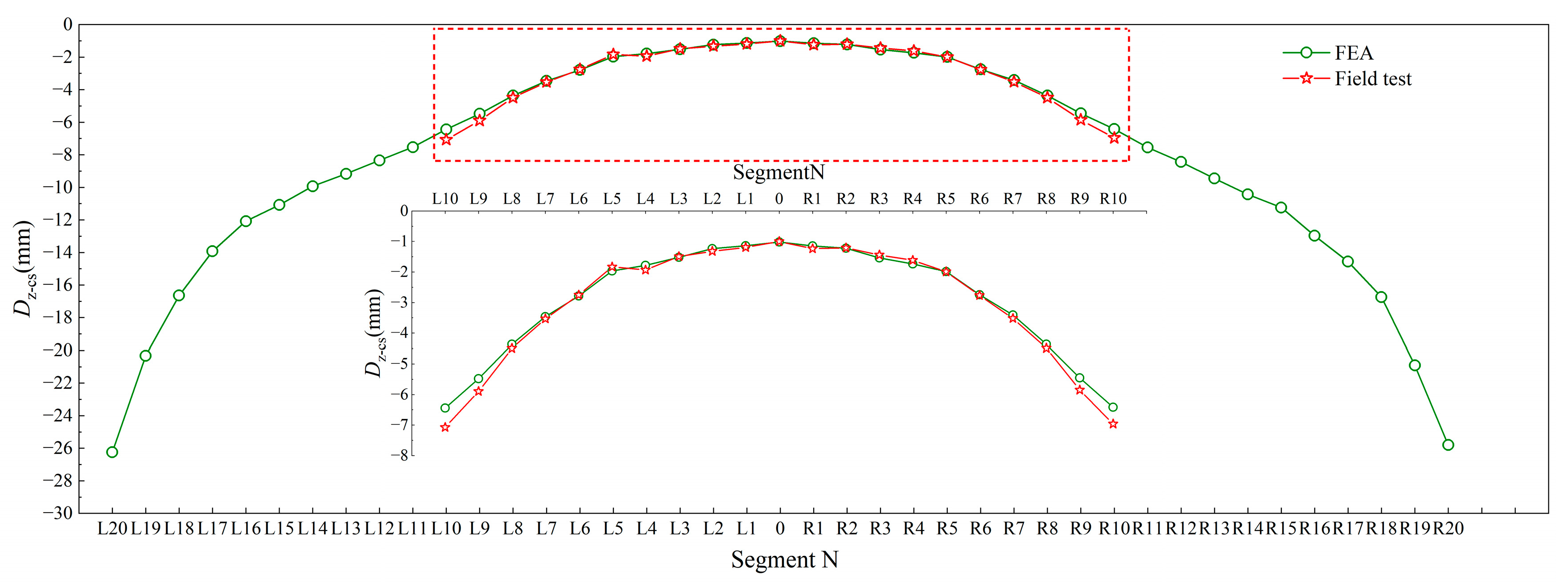
The model accounts for dead loads, including the self-weights of structural members, the self-weight of the hanging scaffold (modelled as concentrated loads), temporary loads (modelled as uniformly distributed loads), the initial tension of the prestressing tendon, and the temperature loads that affect the structure. Actual boundary conditions were modelled by fixing all degrees of freedom at the pier bases [37]. Notably, a linear elastic material model was adopted in the finite element analysis. This assumption is reasonable because the deflection of cantilever segments was evaluated within short construction intervals (approximately 24–48 h between successive segment castings), during which time-dependent effects such as creep and shrinkage have only a minor influence. According to field monitoring, the ambient temperature variation during the actual construction period was within approximately ±5 °C, indicating limited thermal gradients and negligible thermal curvature. Nevertheless, to examine a broader range of possible conditions, the orthogonal experimental design (Section 3.3) considered temperatures ranging from 2.5 °C to 27.5 °C. The close agreement between the predicted and measured deflections verifies that these simplifications provide sufficient accuracy for the present analysis. Field deflections were measured using a Leica TS60 high-precision total station equipped with reflective prisms installed at the tip of each cantilever segment. Measurements were repeated three times for each segment during the concrete curing stage and averaged to reduce random errors. The measurement accuracy was within ±0.5 mm, which ensured reliable validation of the numerical predictions presented in Figure 4. The computations were carried out on a system that was equipped with an Intel Xeon E5-2680 2.4 GHz processor and 64 GB of memory. A single finite element model run consumed approximately 0.5 h of CPU time, thus indicating a high computational cost. Finite element model parameters were iteratively adjusted to reflect actual construction conditions while balancing computational efficiency and accuracy. Hence, the adaptive MEC–RBF method offers practical guidance for bridge construction management.
Model accuracy was assessed through a comparison of field test and finite element results for segmental deflections during construction (DZ-CS), as shown in Figure 4. The analysis results are in good agreement with the measured deflections of the completed 10 segments. A maximum error of 0.8 mm was observed between the finite element results and field data. However, as the cantilever length L increased, the finite element analysis effects became more pronounced in the unconstructed segments, segments #11 to #20. Specifically, the DZ-CS value for segment #20 differs from that of segment #9 by approximately 19 mm, which indicates the necessity of deflection prediction for unfinished segments [38].

3.3. Parameter Selection and Sensitivity Analysis

A sensitivity analysis was performed to assess the importance of the input parameters, with the aims of reducing the computational load and increasing the efficiency of the adaptive MEC–RBF model [39]. In this study, eight parameters with significant variations during the construction of the prestressed concrete continuous rigid frame bridge were considered [40]. These parameters included the Young’s modulus values of the concrete and steel, E c and E s , respectively; the densities of the concrete and steel, γ c and γ s , respectively; the tensile stress of the prestressed tendon, σ ; the structural temperature, T ; the uniformly distributed load, P ; and the ratio of the beam segment length to the cantilever length, d / L .
The range (Rj), which was used as the sensitivity index for evaluating the orthogonal experimental results, is defined in Table 1 as follows:
R j = max K 1 j , K 2 j , min K 1 j , K 2 j ,
K i j = 1 n k = 1 n Y k
where K i j represents the average value of parameter j at level i, n represents the number of trials, and Yk represents the ith value of DZ-CS.
The calculation results are presented in Figure 5. According to these results, d/L is the parameter that has the greatest influence on the response of DZ-CS, followed by σ , γ c , γ s , E c and E s , which also have significant effects. Parameters P and T were insignificant, which is attributed mainly to the relatively small temperature gradients observed during the construction period. Although the ambient temperature levels explored in the orthogonal design ranged from 2.5 °C to 27.5 °C, representing an extended envelope for analysis, the corresponding thermal curvature remained minor compared with the effects of self-weight, prestressing, and construction sequencing. These findings are consistent with the justification provided in Section 3.2 and indicate that temperature influences play a secondary role in short-term construction deflection. The model, however, can be readily retrained with augmented temperature data should a project experience larger gradients or seasonal variations. Thus, the neural network inputs were narrowed to six parameters: d / L , σ , γ c , γ s , E c , and E s . Notably, the range-based index (Rj) adopted in this study reflects only the first-order (main) effects of each input variable and does not explicitly capture potential interactions among variables. Nevertheless, the method provides an intuitive and computationally efficient means to identify the dominant parameters influencing bridge deflection. Future work will extend the analysis using variance-based techniques such as the Sobol or Morris sensitivity methods to quantify higher-order interaction effects.

3.4. Adaptive MEC–RBF Neural Network Prediction Model

3.4.1. Model Construction

Developed in Python 3.12.7, the adaptive MEC–RBF prediction model was trained according to the procedure described in Section 3.3. Multiple training parameters, as listed in Table 2, were employed in the experimental setup to develop the adaptive MEC–RBF model.
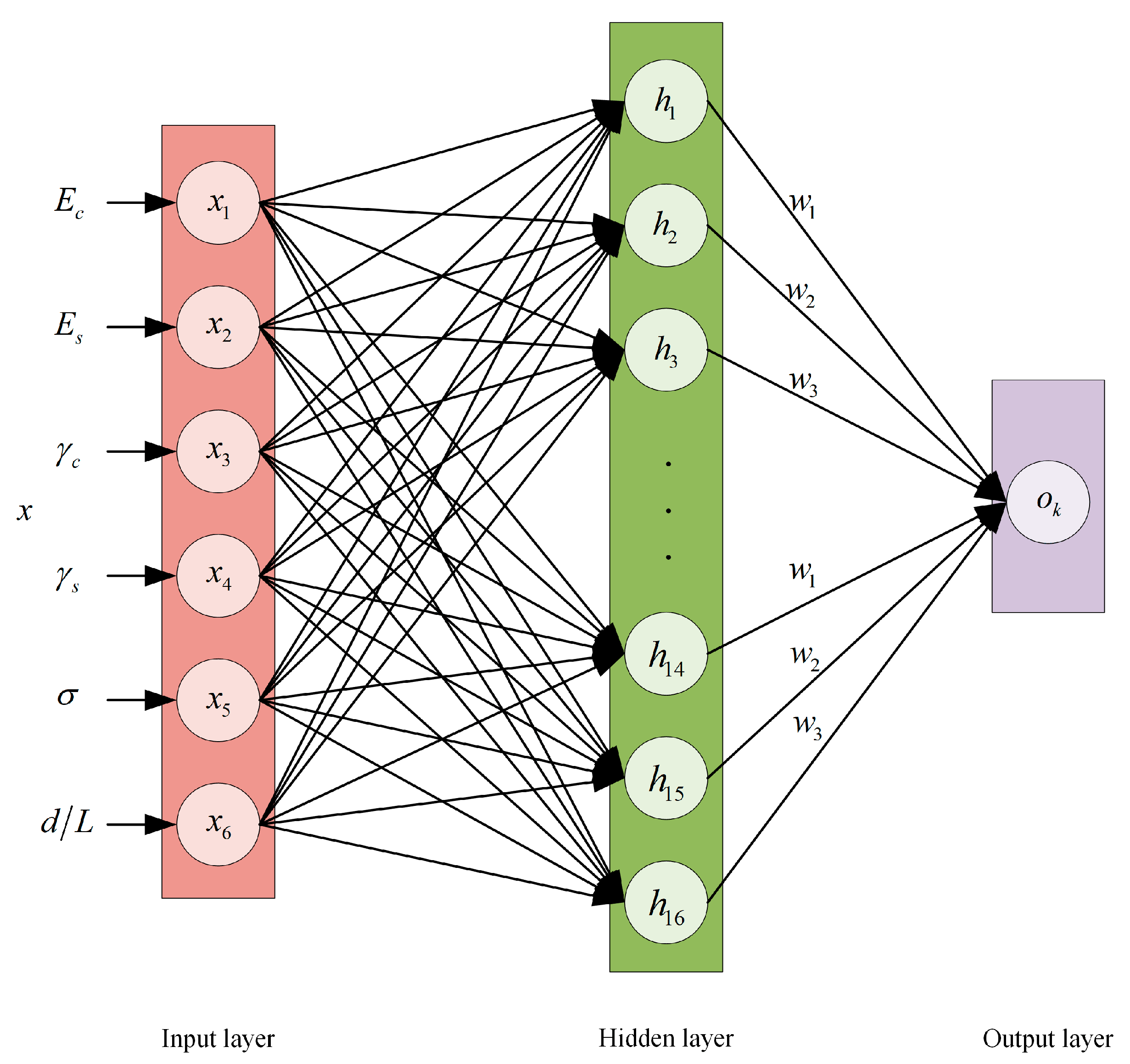
The RMSE values of the adaptive MEC–RBF models with various architectures are shown in Figure 6. The RMSE decreased as the number of hidden neurons increased and reached a minimum at 16 neurons with a population size of M = 500. Thus, the 6–16–1 architecture with M = 500 was chosen as the optimal model, as illustrated in Figure 7.
Considering the probabilistic properties of the variables listed in Table 3, 300 input samples were randomly generated via Latin hypercube sampling (LHS) techniques for analysis. Among these 300 input samples, five levels of d/L (0.063, 0.060, 0.056, 0.053, and 0.051) were randomly distributed. The corresponding output samples were derived from the validated finite element model calculations.
The statistical properties of the input samples (excluding d/L) are shown in Figure 8. Among them, 250 samples were used for training, and 50 were used for testing the adaptive MEC–RBF model. To further verify the robustness and generalizability of the adaptive MEC–RBF model, a fivefold cross-validation procedure was performed. The entire dataset of 300 samples was randomly partitioned into five equal subsets, where four subsets were used for training and one was used for testing in each run. The process was repeated five times so that every subset was used once as the testing set. The mean coefficient of determination (R2) across the five folds was 0.972, and the corresponding mean RMSE was 2.18 mm, indicating that the model maintained stable performance on unseen data without significant overfitting. The average training time of the adaptive MEC–RBF model was approximately 138 s, which represented a substantial reduction compared with that of the finite element analysis, which required approximately 0.5 h per run. Once trained, the MEC–RBF model generated deflection predictions in less than 1 s, confirming its capability for near-real-time application in construction control.

3.4.2. Model Validation

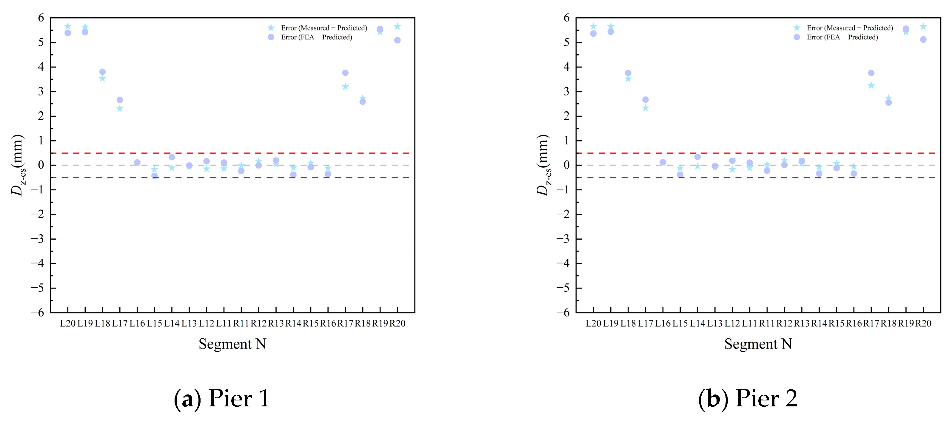
The performance of the adaptive MEC–RBF model was compared with that of the conventional RBF model during the training and testing phases, as shown in Figure 9a and 9b, respectively. The residual distributions illustrated in Figure 10a,b reveal that most residuals lie within ±0.5 mm and are randomly scattered around zero, confirming the model’s stability and the absence of systematic bias. These results demonstrate that, in both phases, the DZ–CS values predicted by the adaptive MEC–RBF model exhibit much closer agreement with those obtained from the finite element simulations. Moreover, based on the comparison between the adaptive MEC–RBF and FEM-derived DZ–CS results, the average prediction error of the adaptive MEC–RBF model was less than 5%, significantly outperforming the conventional RBF model. This clearly confirms the superiority of the adaptive MEC–RBF model over the traditional RBF approach.
Furthermore, the evaluation metrics [41] for both the adaptive MEC–RBF model and the conventional RBF model are presented in Table 4. On the training samples, the adaptive MEC–RBF model achieved a coefficient of determination R2 = 0.9789, an RMSE of 1.4978, and an MAE of 0.1411. On the testing samples, R2 = 0.9751, the RMSE was 1.9491, and the MAE was 0.2341. In terms of all the metrics, the adaptive MEC–RBF model outperformed the conventional RBF model. These results confirm that the adaptive MEC–RBF model offers superior efficiency and accuracy, which makes it well suited for deflection prediction. To further evaluate the significance of the performance improvement achieved by the adaptive MEC–RBF model, a paired t test was conducted on the prediction errors obtained from the adaptive MEC–RBF and conventional RBF models. The resulting p value (<0.05) indicates that the difference in performance between the two models is statistically significant. This confirms that the observed improvement is not due to random variation but reflects the enhanced learning capability of the adaptive mechanism.

3.4.3. Analysis and Discussion of the Results

The application of the trained adaptive MEC–RBF model to the Hannam Yangtze River Bridge yielded accurate deflection predictions. As illustrated in Figure 11a,b, the predicted DZ-CS values obtained by the adaptive MEC–RBF model on the basis of field-measured input parameters are in near-perfect agreement with the finite element analysis results across most cantilever segments. Most residuals lie within ±0.5 mm and are randomly scattered around zero in Figure 12a,b. The maximum discrepancy between the adaptive MEC–RBF model predictions and the measured field deflections of the Hannan Yangtze River Bridge was 5.56 mm, corresponding to a 17.7% relative error. These findings confirm that the proposed model provides satisfactory accuracy for engineering applications. Given the complexity of the construction environment and the effectiveness of the neural network, this accuracy is acceptable for practical deflection control.

4. Conclusions

To increase control efficiency and prediction accuracy when construction schedules are complex and time-constrained and large-scale finite element analyses of intricate bridge structures are required, this study proposes a deflection prediction framework that integrates sensitivity analysis with an adaptive MEC–RBF neural network. The main contributions of this research are summarized as follows:
  • The sensitivity analysis revealed that the parameter d / L had the greatest influence on segment deflection, followed by the parameters σ , γ c , γ s , E c , and E s , whereas the other parameters exhibited relatively minor effects.
  • A comparison with finite element analysis revealed that the adaptive MEC–RBF model achieved higher accuracy and computational efficiency than the conventional RBF model did, providing more precise deflection predictions during construction.
  • Application of the adaptive MEC–RBF model to the Hannan Yangtze River Bridge demonstrated that its predictions were in good agreement with field measurements, confirming the accuracy and practical applicability of the proposed framework. These findings suggest that the approach can effectively support deflection control for prestressed concrete continuous rigid-frame bridges.
The adaptive MEC–RBF framework was validated using data from the Hannan Yangtze River Bridge. It can be retrained and applied to other continuous rigid-frame or prestressed concrete bridges by updating the input parameters and training datasets. Although this flexibility allows the proposed model to serve as a general framework for deflection prediction during construction, several limitations remain and will be addressed in future studies. Verification of data reliability is required during the dataset generation phase, so the finite element model may require adjustments and lead to additional computational costs. Moreover, given the complexity of bridge construction, the probabilistic characteristics of variables may vary under different practical conditions. Future work will focus on extending the adaptive MEC–RBF model to stress prediction in prestressed concrete continuous rigid-frame bridges and comparing its performance with that of other hybrid optimization models, such as particle swarm optimization and grey wolf optimizer–radial basis function neural networks. In addition, the proposed model was developed and validated within a temperature range covered by both field observations (±5 °C) and an orthogonal experimental design (2.5–27.5 °C). For bridge projects subjected to wider temperature variations or pronounced through-depth thermal gradients, the same framework can be extended by incorporating additional temperature data to preserve predictive accuracy.

Author Contributions

Conceptualization, Q.G.; methodology, Q.G. and L.S.; software, Q.H.; validation, C.Z. and L.S.; formal analysis, Q.H. and D.T.; investigation, C.Z. and D.T.; resources, C.Z. and L.S.; data curation, Q.H. and D.T.; writing—original draft preparation, Q.G.; writing—review and editing, C.Z., Q.G., Q.H., L.S. and D.T.; visualization, Q.H.; supervision, Q.G. and D.T.; project administration, C.Z.; funding acquisition, Q.G. All authors have read and agreed to the published version of the manuscript.

Funding

This research received no external funding.

Institutional Review Board Statement

Not applicable.

Informed Consent Statement

Not applicable.

Data Availability Statement

The data, finite-element models, and codes that support the findings of this study are available from the corresponding author upon reasonable request.

Conflicts of Interest

Authors Liangbo Sun and Dewei Tian were employed by the company The First Company of China Eighth Engineering Division Ltd. The remaining authors declare that the research was conducted in the absence of any commercial or financial relationships that could be construed as a potential conflict of interest.

Abbreviations

The following abbreviations are used in this manuscript:
MECMind evolutionary computation
RBFRadial basis function
R2Coefficient of determination
RMSERoot mean square error
MAEMean absolute error

References

  1. Petroski, H. Engineering: Infrastructure. Am. Sci. 2009, 97, 370–374. [Google Scholar] [CrossRef]
  2. Perez, A.I.; Ardaman, A.K. New infrastructure: Civil engineer’s role. J. Urban Plan. Dev. 1988, 114, 61–72. [Google Scholar] [CrossRef]
  3. Ge, Y.; Xiang, H. Concept and requirements of sustainable development in bridge engineering. Front. Archit. Civ. Eng. China 2011, 5, 432–450. [Google Scholar] [CrossRef]
  4. Paunova, D.; Tzonevska, D. Strategic development of the national road network. IOP Conf. Ser. Mater. Sci. Eng. 2023, 1297, 012016. [Google Scholar] [CrossRef]
  5. Peng, Y.; Zhang, Z. Development of a novel type of open-web continuous reinforced-concrete rigid-frame bridge. J. Bridge Eng. 2020, 25, 05020005. [Google Scholar] [CrossRef]
  6. Zhang, S.; Yu, B.; Li, R. Research on the intelligent construction and development of bridge engineering safety management. E3S Web Conf. 2024, 565, 03013. [Google Scholar] [CrossRef]
  7. Yang, J.; Xiang, F.; Li, R. Intelligent bridge management via big data knowledge engineering. Autom. Constr. 2022, 135, 104118. [Google Scholar] [CrossRef]
  8. Zhang, J.; Liu, L.; Yang, H. An overview of intelligent construction and maintenance technology for highway subgrade engineering. Intell. Transp. Infrastruct. 2023, 2, liad019. [Google Scholar] [CrossRef]
  9. Carbonari, S.; Nicoletti, V.; Martini, R.; Gara, F. Dynamics of bridges during proof load tests and determination of mass-normalized mode shapes from OMA. Eng. Struct. 2024, 310, 118111. [Google Scholar] [CrossRef]
  10. Ferrara, M.; Bertagnoli, G.; Giordano, L. Model updating of different bridge types using ambient vibration and OMA identification. Procedia Struct. Integr. 2024, 62, 773–780. [Google Scholar] [CrossRef]
  11. Li, X.; Wang, M.; Liang, Y. Research into design and construction key technologies of prestressed concrete continuous rigid frame bridge. In Proceedings of the 2011 IEEE International Conference on Remote Sensing, Environment and Transportation Engineering, Nanjing, China, 24–26 June 2011; pp. 617–621. [Google Scholar]
  12. Li, H.; Huang, Y.; Guo, E. Construction stage seismic vulnerability evaluation of a continuous girder bridge with the cast-in-place cantilever construction method. Adv. Civ. Eng. 2021, 2021, 9915947. [Google Scholar] [CrossRef]
  13. Zhou, Y. Pre-camber control of large-span prestressed concrete continuous rigid-frame bridges under cantilever construction. Arch. Civ. Eng. 2025, 71, 469–487. [Google Scholar] [CrossRef]
  14. Zhou, X.; Deng, T.; Chen, L. Application of Bayesian update method in the construction control of continuous rigid frame bridge girders with high piers and large spans. Buildings 2023, 13, 1556. [Google Scholar] [CrossRef]
  15. Wan, L.; Qiao, J.; Sun, Q.; Liu, J. Construction control of rigid frame-continuous girder bridge based on grey theory. J. Eng. Appl. Sci. 2024, 71, 171. [Google Scholar] [CrossRef]
  16. Dong, F.; Shi, Z.; Zhong, R. FE model updating of continuous beam bridge based on response surface method. Buildings 2024, 14, 960. [Google Scholar] [CrossRef]
  17. Wang, X.G.; Ma, M.; Zhao, B. Response surface model optimization algorithm for structural assessment based on vibration frequency. Shock Vib. 2025, 2025, 5446251. [Google Scholar] [CrossRef]
  18. Kovačević, M.; Ivanišević, N.; Stević, D. Decision-support system for estimating resource consumption in bridge construction based on machine learning. Axioms 2022, 12, 19. [Google Scholar] [CrossRef]
  19. Pan, Y.; Zhang, L. Integrating BIM and AI for smart construction management: Current status and future directions. Arch. Comput. Methods Eng. 2023, 30, 1081–1110. [Google Scholar] [CrossRef]
  20. Zhu, H.; Wang, Y. Intelligent prediction of prestressed steel structure construction safety based on BP neural network. Appl. Sci. 2022, 12, 1442. [Google Scholar] [CrossRef]
  21. Li, Q.; Xie, J. Bridge alignment prediction based on combination of grey model and BP neural network. Appl. Sci. 2024, 14, 7955. [Google Scholar] [CrossRef]
  22. Wang, X.; Miao, C.; Wang, X. Prediction analysis of deflection in the construction of composite box-girder bridge with corrugated steel webs based on MEC-BP neural networks. Structures 2021, 32, 691–700. [Google Scholar] [CrossRef]
  23. Yang, Y.; Xia, X.; Lo, D. Predictive models in software engineering: Challenges and opportunities. ACM Trans. Softw. Eng. Methodol. 2022, 31, 1–72. [Google Scholar] [CrossRef]
  24. Liao, S.; Li, S.; Liu, J. A zeroing neural dynamics-based acceleration optimization approach for optimizers in deep neural networks. Neural Netw. 2022, 150, 440–461. [Google Scholar] [CrossRef] [PubMed]
  25. Mao, Y.; Ma, Z.; Liu, X. A long-term prediction method of computer parameter degradation based on curriculum learning and transfer learning. Mathematics 2023, 11, 3098. [Google Scholar] [CrossRef]
  26. Zhang, Z. Pattern classification based on radial basis function neural network. In Proceedings of the 2020 IEEE 5th International Conference on Smart Grid and Electrical Automation (ICSGEA), Zhangjiajie, China, 13–14 June 2020; pp. 213–216. [Google Scholar]
  27. Dai, Y.; Wu, Q.; Zhang, Y. Generalized sparse radial basis function networks for multi-classification problems. Appl. Soft Comput. 2024, 154, 111361. [Google Scholar] [CrossRef]
  28. Chen, S.; Bai, W. Performance analysis of typical linear augmented observers for a class of MIMO systems with nonlinear uncertainty. ISA Trans. 2022, 128, 316–327. [Google Scholar] [CrossRef]
  29. He, X.J.; Zeng, J.C.; Jie, J. Artificial neural network weights optimization design based on MEC algorithm. In Proceedings of the 2004 IEEE International Conference on Machine Learning and Cybernetics, Shanghai, China, 26–29 August 2004; Volume 6, pp. 3361–3364. [Google Scholar]
  30. Jie, J.; Zeng, J.; Zhang, S.L. Mind evolutionary computation for the constrained optimization. In Proceedings of the IEEE 2002 International Conference on Machine Learning and Cybernetics, Beijing, China, 4–5 November 2002; Volume 3, pp. 1582–1585. [Google Scholar]
  31. Sun, C.; Wang, J. Performance of MEC in high-dimensional space. In Proceedings of the 2002 IEEE International Conference on Control and Automation (ICCA), Xiamen, China, 19 June 2002; p. 231. [Google Scholar]
  32. Qin, J.; Huang, C.; Luo, Y. Adaptive multi-swarm in dynamic environments. Swarm Evol. Comput. 2021, 63, 100870. [Google Scholar] [CrossRef]
  33. Wang, H.; Yang, S. Memetic algorithms for dynamic optimization problems. In Evolutionary Computation for Dynamic Optimization Problems; Springer: New York, NY, USA, 2013; pp. 137–170. [Google Scholar]
  34. Helton, J.C.; Davis, F.J. Latin hypercube sampling and the propagation of uncertainty in analyses of complex systems. Reliab. Eng. Syst. Saf. 2003, 81, 23–69. [Google Scholar] [CrossRef]
  35. Zheng, B. Parametric modeling and finite element analysis of the camshaft based on ANSYS APDL. In Proceedings of the 2018 IEEE 4th Information Technology and Mechatronics Engineering Conference (ITOEC), Chongqing, China, 14–16 December 2018; pp. 1805–1808. [Google Scholar]
  36. Nie, J.G.; Zhu, L. Beam-truss model of steel–concrete composite box-girder bridges. J. Bridge Eng. 2014, 19, 04014023. [Google Scholar] [CrossRef]
  37. Zhang, W.; Chang, J.; Tian, G. FEM-based shape-finding and force-assessment of suspension bridges via completed loop adjustment. J. Bridge Eng. 2022, 27, 04021098. [Google Scholar] [CrossRef]
  38. Li, J.; Li, D.; Li, F. Finite element analysis of displacement and vibration characteristics of cantilevered plate. J. Phys. Conf. Ser. 2020, 1578, 012241. [Google Scholar] [CrossRef]
  39. Zhao, T.; Zheng, Y.; Wu, Z. Improving computational efficiency of machine-learning modeling of nonlinear processes using sensitivity analysis and active learning. Digit. Chem. Eng. 2022, 3, 100027. [Google Scholar] [CrossRef]
  40. Hisam, M.W.; Dar, A.A.; Elrasheed, M.O. The versatility of the Taguchi method: Optimizing experiments across diverse disciplines. J. Stat. Theory Appl. 2024, 23, 365–389. [Google Scholar] [CrossRef]
  41. Tong, Y.L. The Multivariate Normal Distribution; Springer: New York, NY, USA, 2012. [Google Scholar]
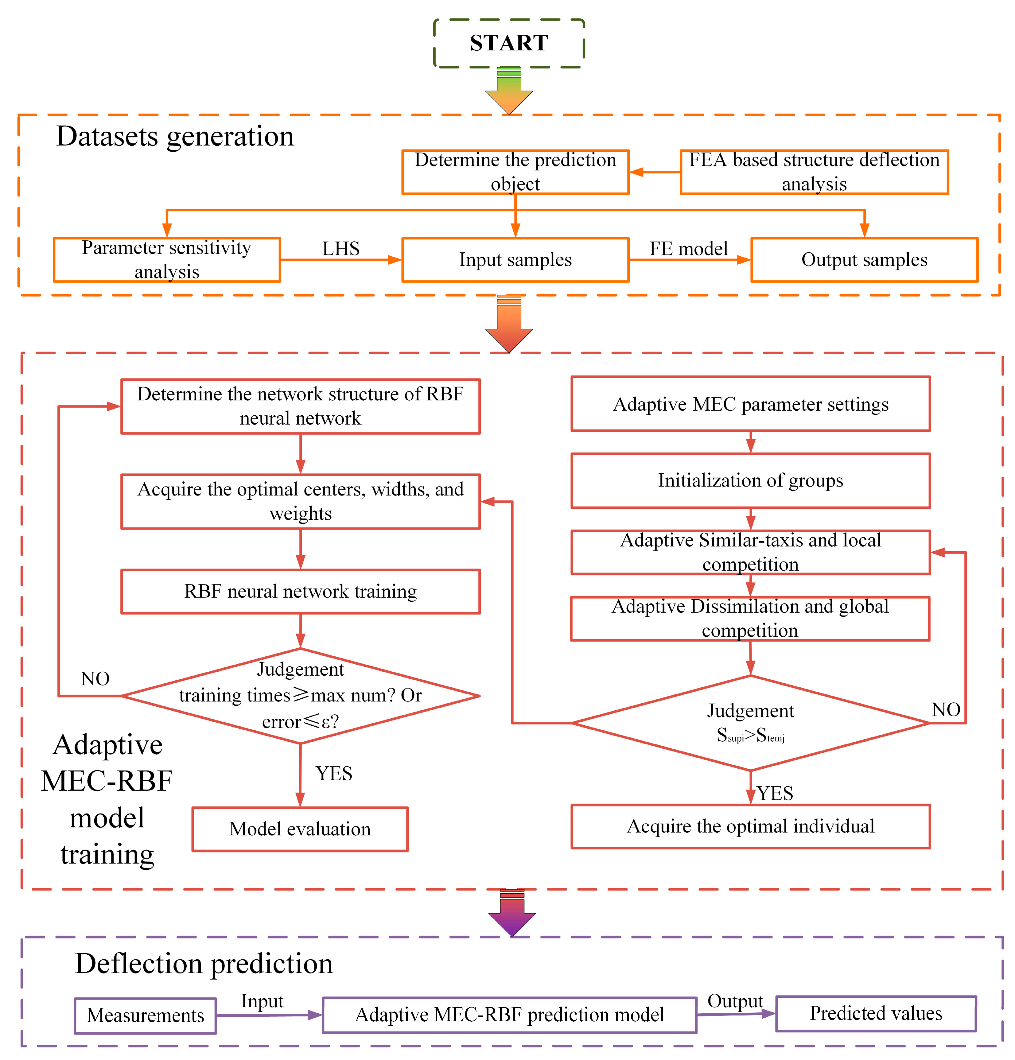
Figure 1. Framework of the adaptive MEC–RBF neural network for deflection prediction.
Applsci 15 11326 g001
Figure 2. Hannan Yangtze River Bridge.
Applsci 15 11326 g002
Figure 3. Finite element model.
Applsci 15 11326 g003
Figure 4. Comparison of segmental deflections during the concrete casting stage.
Applsci 15 11326 g004
Figure 5. Histogram of Rj.
Applsci 15 11326 g005
Figure 6. Performance of the adaptive MEC–RBF model at various N2 values.
Applsci 15 11326 g006
Figure 7. Structure of the three-layer RBF neural network.
Applsci 15 11326 g007
Figure 8. Statistical characteristics of the input samples.
Applsci 15 11326 g008
Figure 9. Comparison of the values predicted by the adaptive MEC–RBF and RBF models with the FEA results.
Applsci 15 11326 g009
Figure 10. Comparison of residuals between the adaptive MEC–RBF and conventional RBF models with respect to the FEA results.
Applsci 15 11326 g010
Figure 11. Comparison of cantilever beam deflection development between pier 1 and pier 2.
Applsci 15 11326 g011
Figure 12. Comparison of measured–predicted and FEA–predicted deflection residuals between pier 1 and pier 2.
Applsci 15 11326 g012
Table 1. Orthogonal experimental design and calculation results.
N o . 12345678 D Z C S ( mm )
E c ( GPa ) E s ( GPa ) γ c ( kN / m 3 ) γ s ( kN / m 3 ) σ ( GPa ) P ( kN / m ) d / L T ( C )
11 (25.075)1 (167.25)1 (22.125)1 (67.625)1 (1.2255)1 (3.75)1 (0.063)1 (2.5)−15.08
212 (189.9)2 (23.85)2 (73.25)2 (1.3302)2 (10.5)2 (0.060)2 (10)−19.57
313 (205)3 (25)3 (77)3 (1.40)3 (15)3 (0.056)3 (15)−23.45
414 (220.1)4 (26.15)4 (80.75)4 (1.4698)4 (19.5)4 (0.053)4 (20)−29.57
515 (242.75)5 (27.875)5 (86.375)5 (1.5745)5 (26.25)5 (0.051)5 (27.5)−31.55
62 (29.47)1234512−4.06
722345123−6.28
823451234−48.87
924512345−56.85
1025123451−38.60
113 (32.4)1352441−43.92
1232413552−50.58
1333524113−23.80
1434135224−10.34
1535241335−35.86
164 (35.33)1425353−35.12
1742531414−28.00
1843142525−19.88
1944253131−23.78
2045314242−28.50
215 (39.725)1543243−38.57
2252154354−22.32
2353215415−6.61
2454321521−28.49
2555432132−32.39
2611145432−17.83
2712251543−55.68
2813312154−60.21
2914423215−25.18
3015534321−33.01
3121213324−22.85
3222324435−28.91
3323435541−35.53
3424541152−72.53
3525152213−17.35
3631331255−50.93
3732442311−22.79
3833553422−31.22
3934114533−18.86
4035225144−20.02
4141454125−20.28
4242515231−26.04
4343121342−31.25
4444232453−42.37
4545343514−17.00
4651522534−37.19
4752133145−18.28
4853244251−26.76
4954355312−9.34
5055411423−30.52
K 1 −311.13−285.81−209.79−316.10−397.21−292.64−169.21−293.98
K 2 −331.83−278.44−257.55−288.11−352.50−292.11−222.44−297.27
K 3 −308.32−307.58−297.02−278.35−289.50−292.83−293.18−291.99
K 4 −272.22−317.32−330.83−287.07−236.07−297.56−358.16−296.38
K 5 −250.46−284.80−378.76−304.32−198.67−298.81−430.96−294.32
R j 8.143.8916.903.7819.850.6726.180.53
Table 2. Parameter settings of the adaptive MEC–RBF model.
AlgorithmParameterDefinitionLevels
Adaptive MECMThe population size100, 200,…, 500
MsupThe superior group size6
MtemThe temporary group size6
ImaxThe maximum number of iterations300
RBFN1The number of neurons in the input layer6
N2The number of neurons in the hidden layer4,…, 18
N3The number of neurons in the output layer1
epThe number of iterations600
GThe training accuracy1 × 10−5
Table 3. Properties of random variables.
VariableMean μ Standard Deviation σ Distribution TypeRemarks
E c 32.42.93Normal distributionYoung’s modulus (concrete)
E s 20515.1Normal distributionYoung’s modulus (steel)
γ c 251.15Normal distributionDensity (concrete)
γ s 773.75Normal distributionDensity (steel)
σ 1.400.0698Normal distributionPrestressing tendon tensile stress
T 154.5Normal distributionStructural temperature
P 70032.5Normal distributionUniformly distributed load
Table 4. Statistical metrics of the DZ-CS prediction model.
ModelTraining SamplesTesting Samples
R2RMSEMAER2RMSEMAE
Adaptive MEC–RBF0.97891.49780.14110.97511.94910.2341
RBF0.97112.78690.42110.96793.18070.5678
Disclaimer/Publisher’s Note: The statements, opinions and data contained in all publications are solely those of the individual author(s) and contributor(s) and not of MDPI and/or the editor(s). MDPI and/or the editor(s) disclaim responsibility for any injury to people or property resulting from any ideas, methods, instructions or products referred to in the content.