EvoSMS: An Event-Oriented Simulation Method for Multi-Core Real-Time Scheduling

Abstract

In this paper, an event-oriented simulation analysis approach was established for the schedulability analysis of multi-core embedded systems. To the best of our knowledge, this work is the first to introduce an event-oriented simulation strategy into multi-core processor schedulability analysis. The proposed method transforms the conventional step-by-step simulation into a jump-based simulation process, thereby reducing redundant system state updates and improving computational efficiency. Task execution is abstracted as a time-axis folding operation, and two algorithms, RBTF and PBTF, are developed to optimize event generation and management, effectively lowering the algorithmic complexity of the simulation. Furthermore, to resolve core-mapping conflicts arising in global scheduling during jump-based simulation, a time-axis-unfolding-based dynamic core-mapping algorithm is proposed. By incorporating a time interval recycling mechanism and a priority inheritance algorithm, this method ensures correct job-to-core assignment and enables precise response time analysis under global scheduling policies. This approach reduced the simulation time by 96.24% on average while guaranteeing the accuracy and soundness of the analysis. It is primarily applicable to periodic tasks with implied deadlines, and future work will explore extending this method to support sporadic tasks and tasks with arbitrary deadlines.

1. Introduction

In contrast to single-core computing platforms, multi-core processors offer superior computational performance and exhibit distinct advantages in terms of size, weight, power, and cost (SWaP-C). Because of resource sharing and competition, inter-task parallelism, and other factors in multi-core embedded systems, schedulability analysis methods developed for single-core processors cannot be directly applied to multi-core platforms.

The schedulability verification of multi-core real-time systems typically involves two primary approaches: the analysis-based approach and the simulation-based approach. Over the past five decades, the analysis-based approach has yielded substantial research outcomes. Commencing with the initial utilization analysis centered on processors, advancements have been made, culminating in contemporary response time analysis grounded in schedule–abstraction graphs (SAGs). These strides have significantly enhanced the accuracy of schedulability analysis. Well-known techniques include global EDF scheduling and multiprocessor schedulability tests, which provide formal guarantees under certain assumptions. However, these methods often rely on conservative worst-case assumptions and may yield pessimistic results, limiting their applicability to dynamic or probabilistic workloads commonly encountered in embedded multi-core systems.

The simulation-based approach is another significant method for schedulability analysis, with related tools including SimSo, MCRTsim, and Cheddar, as well as commercial tools such as RapiTime 3.15 and MATLAB 2024a. Simulation-based analysis approaches are usually divided into two categories: process-oriented simulation and event-oriented simulation. The process-oriented simulation approach typically operates in a clock-driven manner, with the simulation clock advancing one step per time slice. However, this approach may encounter inefficiencies when striving for high simulation accuracy or when dealing with a substantial simulation interval. One possible approach is to use events in the system as drivers and execute one simulation every time an event arrives. The event-oriented simulation approach circumvents the necessity of conducting simulations at every time slice, consequently mitigating time wastage.

Compared with existing analysis-based and simulation-based methods, EvoSMS aims to combine the advantages of event-driven simulation with multi-core scheduling-specific optimizations. While traditional global EDF or multiprocessor tests provide formal guarantees, they are often limited in scalability and in capturing detailed system interactions. Existing simulators, on the other hand, frequently rely on process-oriented simulation, which may be inefficient for large-scale scenarios. EvoSMS addresses these gaps by supporting event-driven simulation and flexible multi-core scheduling strategies, thus providing a more accurate and efficient framework for evaluating the schedulability of real-time tasks in complex multi-core systems.

The main contents and contributions of the present research are as follows:

1.

We introduced an approach for modeling a multi-core embedded system, which relies on an “actor-script-scenario” framework. This approach provided a formal definition of system simulation and offered insight into the system’s operational scenarios.

2.

The concept of time-axis folding and unfolding was proposed, which was applied to the schedulability analysis. The folding algorithms PBTF and RBTF were implemented for single-core scheduling algorithms, respectively.

3.

It was discovered that the RBTF algorithm can encounter core-mapping conflicts when applied to multi-core scheduling simulations. A time-axis-unfolding-based dynamic core-mapping algorithm was proposed to address this issue, ultimately leading to the development of the multi-core schedulability simulation algorithm, EvoSMS.

4.

In this paper, the superiority of the approach in terms of analysis accuracy and simulation efficiency was verified through a series of experiments.

The rest of this paper is organized as follows: Section 2 discusses the related studies. Section 3 introduces the system model and simulation definition based on the “actor-script-scenario” framework. We introduce response time analysis algorithms based on time-axis folding and unfolding in Section 4 and Section 5. Section 6 presents three experimental results from the evaluation of the proposed method. Finally, Section 7 concludes the paper and presents future work.

2. Related Work

Schedulability analysis stands as a pivotal concern in the design phase of embedded real-time systems, playing a crucial role in guaranteeing the accuracy of system timing [1,2]. Such analysis has remained a prominent and continuously evolving research subject in the field of real-time systems. Schedulability analysis was brought about by C. L. Liu et al. [3] in 1973 and has progressed to encompass contemporary response time analysis techniques, particularly in the context of real-time quantum computing systems [4].

Over the past 50 years, a number of notable results have been achieved in analysis-based schedulability research. C. L. Liu et al. [3] proposed a schedulability analysis approach based on resource utilization bounds and critical instant, which can be used to determine the schedulability of tasks set considerably efficiently. At the same time, resource utilization is also a vital metric for evaluating scheduling algorithms. Research results have revealed that, assuming the number of tasks in the task set is m and the resource utilization $U=m\times (2^{{\displaystyle \frac{1}{m}}}-1)$ for a single-processor RMS scheduling algorithm, the upper bound of the resource utilization of the RMS scheduling algorithm is 69.3%. A response-time-based analysis technique was proposed by M. Joseph et al. [5]. The approach introduced the concept of “k-busy period” for analyzing the worst-case response time (WCRT) of task ${\tau }_k$ with constrained deadlines, which can be computed by fixed-point iteration. The challenge of response time analysis for tasks with arbitrary deadlines was initially tackled by J. P. Lehoczky et al. [6]. In a subsequent development, N. Audsley et al. [7] extended this work to address the uncertainty associated with task release times, introducing an approach to compute the WCRT that accommodates task release jitter. M. Cünzel et al. [8] explored the field of schedulability tests for self-suspended tasks with arbitrary deadlines and release time jitter, providing comprehensive judgment criteria for task feasibility. In a different vein, T. P. Baker et al. [9] introduced the problem window approach as a novel method for computing multiprocessor response times. This approach obviates the need to enumerate all time windows by instead calculating the maximum workload and interference levels for a task within a given time frame. M. Bertogna et al. [10] identified that if the load of an interference task was excessively large, the portion of the task executed in parallel with the task to be analyzed should not be analyzed as interference. Accordingly, the use of the interference time of the task was proposed, rather than the task load, which improved the analysis accuracy. Further, M. Bertogna et al. [11] applied the response time analysis approach to multi-core processor analysis and classified the interference tasks into carry-in and non-carry-in tasks. The precision of the mentioned approach was refined by S. Baruah et al. [12] Building upon this foundation, Guan et al. [13] expanded on the approach initially proposed by M. Bertogna et al. [10], applying it to G-FP schedulability analysis. They introduced a novel interference amount calculation method to enhance the accuracy of the analysis results. In a related development, Y. Sun et al. [14] introduced a “2-parts execution scenario” to further alleviate the pessimistic nature of the interference amount calculation approach. M. Han et al. [15,16] investigated the root causes of pessimism introduced by Guan et al. [13] and made advancements in analysis accuracy by exhaustively enumerating the release patterns of high-priority tasks for task interference amount analysis. Meanwhile, M. Nasri et al. [17] established a precise analysis approach for task response times within schedule–abstraction graphs (SAGs). This approach enhances analysis efficiency through the application of partial-order reduction (POR) [18,19].

Although a considerable amount of progress has been made in analysis-based schedulability research, compared to scheduling simulation, analytical approaches are more pessimistic and have a lower schedulability task set coverage [20]. Simulation methods, on the other hand, can provide approximate values for specific execution scenarios, whereas analytical approaches give results based on the worst-case analysis. In academia, the realm of simulation-based task schedulability analysis has received comparatively limited attention in contrast to analysis-based approaches. This can largely be ascribed to the inherent challenges associated with simulation-based methods, including their lower analysis efficiency and limited scalability. Common simulation tools are shown in

Table 1. Comparison of simulation tools for schedulability analysis of real-time systems.

Tool	Platform	Execution Time Model	Simulation Approach
MAST-1 [21]	Distributed	WCET	Process-oriented
MAST-2 [21]	Distributed	WCET	Process-oriented
JSimMAST	Distributed	Event-oriented	WCET
STORM [22]	Multiprocessor	WCET	Process-oriented
YARTISS [23]	Multiprocessor	Probabilistic	Event-oriented
SimSo [24]	Uni-/Multiprocessor	WCET/Probabilistic	Process-oriented
Cheddar [25]	Uni-/Multiprocessor	WCET	Analytical

.

MAST and its extended versions, MAST-1/MAST-2, provide a comprehensive framework for modeling and analyzing distributed real-time systems. MAST supports response time analysis, sensitivity analysis, and schedulability tests for a wide range of scheduling policies. It is particularly useful for system-level timing verification, though it focuses on analytical evaluation rather than fine-grained event simulation. JSimMAST later introduced a Java-based simulation environment derived from MAST, enabling stochastic analysis and dynamic behavior exploration. However, its simulation granularity is limited by the abstract analytical nature inherited from MAST.

STORM and YARTISS was introduced to simulate multiprocessor scheduling behavior using modular Java architectures. STORM allows modeling of distributed systems and visual inspection of schedules. YARTISS emphasizes extensibility, concurrent simulation, and energy modeling. However, neither STORM nor YARTISS supports multi-core global scheduling, which prevents the dynamic allocation of tasks across different cores.

Cheddar provides a well-established framework for schedulability analysis and visualization. It supports a wide range of scheduling algorithms and performs timing feasibility checks through analytical models. Nevertheless, Cheddar implemented in Ada supports many scheduling algorithms and feasibility tests but mainly performs analytical verification instead of detailed runtime simulation for multi-core scheduling.

SimSo provides a Python-based discrete-event simulation environment that supports various scheduling policies for uniprocessor and multiprocessor systems. Equipped with a graphical interface and easy scripting capabilities for algorithm evaluation, it relies on a time-slice-driven mechanism, which results in significant simulation overhead in fine-grained temporal analysis.

In contrast, the proposed EvoSMS adopts an event-oriented simulation approach that explicitly models task execution preemptions through time folding and unfolding operations. EvoSMS integrates a conflict-aware core-mapping mechanism, enabling high-precision and scalable simulation for multi-core real-time systems.

3. “Actor-Script-Scenario” System Model

We adopt an “actor-script-scenario” framework to model the embedded system and analyze whether the system can satisfy the requirements of the system’s timing relationship under the predefined “scenario” according to the established “actor” and “script”.

3.1. Actor Model

An embedded real-time system consists of a finite set of tasks $\mathrm{\Gamma }=\{{\tau }_1,{\tau }_2,\dots ,{\tau }_n\}$, and each real-time task will generate an infinite sequence of jobs. A task ${\tau }_i\in \mathrm{\Gamma }$ is a tuple $({\pi }_i,J_i,[C_i^{min},C_i^{max}],[T_i^{min},T_i^{max}],D_i)$, where ${\pi }_i$ is the priority, and the smaller the value, the higher the priority, $J_i$ is the release time jitter, $[C_i^{min},C_i^{max}]$ indicates the execution time of the task, $C_i^{min}$ is the best-case execution (BCET), $C_i^{max}$ is the worst-case execution (WCET), and $[T_i^{min},T_i^{max}]$ denotes the time interval between the arrival of two neighboring jobs; if $T_i^{min}=T_i^{max}$, it indicates that the task arrival interval is a fixed value, in which case the task is a periodic task. If only the minimum arrival interval can be determined, then the task is a sporadic task, and $D_i$ is the relative deadline. In this paper, we focus on the periodic task model with an implied deadline, i.e., $T_i^{min}=T_i^{max}=D_i$.

We form a finite job set ${\mathcal{J}}_i=\{{\tau }_{i,1},{\tau }_{i,2},\dots ,{\tau }_{i,n}\}$, where ${\tau }_{i,j}$ denotes the j-th instance of task ${\tau }_i$, each job ${\tau }_{i,j}$ is a tuple $({\pi }_{i,j},r_{i,j},c_{i,j},d_{i,j})$, where ${\pi }_{i,j}$ is the priority of job ${\tau }_{i,j}$, $r_{i,j}$ is the release time, $c_{i,j}\in [C_i^{min},C_i^{max}]$ is the execution of job, and $d_{i,j}$ is the absolute deadline. The task releases jobs periodically with a period from the starting moment of the system, which we assume to be at time $t=0$, calculated release time $r_{i,j}\in [(j-1)\ast T_i,(j-1)\ast T_i+J_i]$, and absolute deadline $d_{i,j}=(j-1)\ast T_i+D_i$.

Compared to traditional models where execution time and period are defined as single values, the proposed model in this paper defines execution time and period as time intervals. This approach allows for a more comprehensive and accurate evaluation of task schedulability analysis.

3.2. Script Model

$Script$ is a task-scheduling algorithm used to arrange and regulate the performance process of $actors$. There are various classification methods for task-scheduling algorithms, such as preemptive and non-preemptive, static priority and dynamic priority, work-conserving and non-work-conserving, etc. This paper focuses on deterministic and memoryless scheduling algorithms [17,26].

Definition 1.

(Deterministic and memoryless scheduler) A scheduler is deterministic and memoryless if, and only if, the scheduling decision at time t is unique and univocally defined by the state of the system at time t.

The typical representative is fixed-priority scheduling (FPS).

Definition 2.

(Fixed-priority scheduler) In a fixed-priority (FPS) scheduler, every task is assigned a fixed priority. The scheduling decision is selecting the tasks to be executed based on their priority.

3.3. Scenario Model

The scenario model describes a possible execution situation of the system, and the scenario model of each task jointly constructs the “scenario” model of the system. Mitra Nasri defined “execution scenarios” in her paper [17]: an execution scenario $\gamma =(C,R)$ for a set of jobs $\mathcal{J}$ is a sequence of execution times $C=\langle C_1,C_2,\dots ,C_m\rangle$ and release times $R=\langle r_1,r_2,\dots ,r_m\rangle$ such that, for each job $J_i$, $C_i\in [C_i^{min},C_i^{max}]$ and $[r_i^{min},r_i^{max}]$.

This definition limits the release time and execution time of the jobs in the system, eliminating the uncertainty of the time parameter. However, this definition has a large degree of duplication with the model of the job and fails to generalize other key parameters during the execution of the system, such as job response time and resource utilization. Therefore, in this paper, we will give the definition of the system execution scenario directly from the perspective of the execution results.

Definition 3.

(System state) The state of the real-time system is the status of task and message execution and resource utilization in the system at this moment.

Definition 4.

(System execution scenario) For an embedded real-time system, its execution scenario is a sequence composed of system states, denoted as $\xi =(S_1,S_2,\dots ,S_n)$, where $S_i\in \xi$ represents the state of the system.

3.4. Simulation Model

According to Rubinstein’s [27] classification of simulation models, we can determine that embedded real-time system models belong to discrete-event dynamic systems (DEDSs). DEDS simulation is the process in which the state changes over time or events, and the simulation results are a collection of system states that change over time or events, namely the system execution scenario. The next state of an embedded real-time system depends on the current system state and system input, as shown in Figure 1.

The input to the embedded real-time system simulation process is the system model and the simulation interval. After simulation, a series of time-varying state sequences are obtained. The simulation process is defined as follows:

$$(sysModel,simInterval)\stackrel{simulation}{\to }\xi$$

(1)

where $sysModel$ is the stochastic model of the system, $simInterval$ represents the simulation interval, and the simulation result is expressed as follows:

$$\xi =\left\{\begin{array}{cc}S\left(0\right),\dots ,S\left(simInterval\right)\hfill & process-oriented\hfill \\ S\left(0\right),\dots ,S\left(even{t}_{last}\right)\hfill & event-oriented\hfill \end{array}\right.$$

(2)

where $\xi$ is the simulation result. For the process-oriented simulation approach, $S\left(i\right)$ denotes the state of the system at time $i\in (0,\dots ,simInterval)$, and the final state of the system is $S\left(simInterval\right)$. For the event-oriented simulation approach, $S\left(i\right)$ denotes the state of the system at the occurrence of event i. In particular, $S\left(0\right)$ denotes the initial state of the system, and $S\left(even{t}_{last}\right)$ denotes the state of the system at the occurrence of the last event.

To characterize a multi-core processor real-time system simulation model, we establish an event-oriented multi-core processor real-time system simulation model, denoted as $f_{mc\_eo}$, based on the system simulation process described by Equation (2). The model is presented as shown in Equation (3).

$$f_{mc\_eo}(Actor,Script,simInterval)=\xi$$

(3)

4. Time-Axis Folding Algorithm and Response Time Analysis

A list of related notations is described in

Table 2. Notations used in the time-axis folding algorithm.

Notations	Description
${\xi }_i=\langle [{\xi }_i^S,{\xi }_i^E],{\pi }_i\rangle$	The folded interval segment, ${\xi }^S$ is the starting point of the time interval, ${\xi }^E$ is the endpoint of the time interval, and ${\pi }_i$ denotes the priority of the time interval
$\mathcal{J}$	The set of jobs
${\mathcal{J}}^{\prime }$	The job set ordered by priority
${\tau }_{i,j}$	The j-th instance of task
$r_{i,j}$	The release time of job ${\tau }_{i,j}$
$c_{i,j}$	The execution time of job ${\tau }_{i,j}$
$J_i$	Task release time jitter
$T_i$	Task period
$top\left({\mathcal{J}}^{\prime }\right)$	The job with the highest priority in ${\mathcal{J}}^{\prime }$
$R_{i,j}$	The response time of job ${\tau }_{i,j}$
$Q_{sus}$	The job pending queue
$PB$	The problem window
$N_P$	The quantity of the process-oriented simulations
$N_E$	The number of simulations
$\eta$	The acceptance ratio of tasks

to facilitate the readability.

4.1. Time-Axis Folding Algorithm

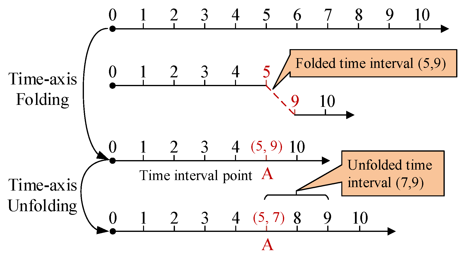
The execution process of a task can be conceptualized as a time-axis folding procedure, with the release time serving as the folding initiation point and the execution duration as the folding duration. With each execution of a task, a segment of time equivalent to the execution time is effectively “removed” from the time axis. From the perspective of time axis, the execution of tasks on a processor can be viewed as a folding process of time intervals. 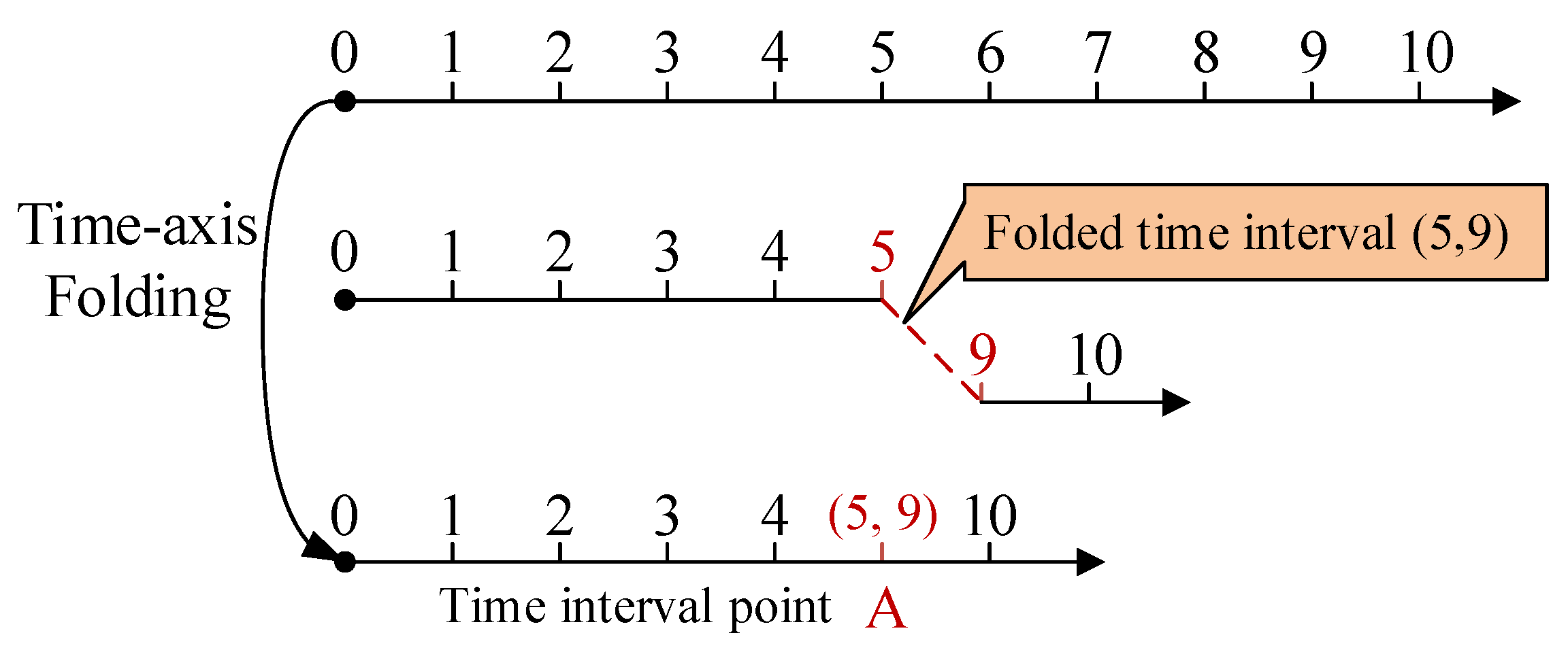Given a time axis $t_0$, the folded time interval collapses into a single point in time. As shown in Figure 2, on the basis of the original time axis, the time interval (5, 9) was folded into a folded interval segment A.

The definition of the folded interval segment is given below.

Definition 5.

(folded interval segment) When a time axis is given, a certain moment is identified as the folding starting point, a fixed duration is identified as the folding duration, and the point-in-time at which folding occurs is referred to as the folded interval segment, denoted as $\xi ({\xi }^S,{\xi }^E)$, where ${\xi }^S$ is the starting point of the time interval, ${\xi }^E$ is the endpoint of the time interval, and the modulus of the folded interval segment $\left|\xi \right|={\xi }^E-{\xi }^S$.

A time axis can be represented as $\{{\xi }_1,{\xi }_1,\dots ,{\xi }_n\}$ by the set of folded interval segments, or ⌀ if a time axis has not undergone any folding. For any time axis, the following rules are followed when performing time-axis folding:

1.

Increase–decrease reciprocity principle: The extent to which the time axis is folded corresponds precisely to the augmented folding duration observed at the folded interval segments.

2.

Principle of folding backward: From the starting point of the folding interval, an equal length of the effective duration is folded backward along the time axis in accordance with the increase–decrease reciprocity principle.

3.

Forward merging principle: When there is an overlap between the folding interval and the folded interval segment on the time axis, the principle of merging should be observed. The folded interval segment is set as ${\xi }_j$, with ${\xi }_i$ being the folded interval segment at the time axis. If the folding starting point is located in $[{\xi }_i^S,{\xi }_i^E]$, then ${\xi }_j^S={\xi }_i^S$. If the folded interval segment is adjacent to the original folded interval segment ${\xi }_i$, namely ${\xi }_j^E={\xi }_i^S$, the two folded interval segments need to be merged forward, namely ${\xi }_j^E={\xi }_i^E$.

According to the aforementioned principle, assuming that the set of folded interval segments of the original time axis is $A=\{{\xi }_1,{\xi }_1,\dots ,{\xi }_n\}$, if a is taken as the folding starting point and $\Delta t$ as the folding duration, the formula for calculating the set B of the time points after the folding can be denoted as shown in Equation (4).

$$B=\left\{\begin{array}{cc}A\cup \widehat{(a,a+\Delta t)},\hfill & \forall {\xi }_i\in A,({\xi }_i^S,{\xi }_i^E)\cap (a,a+\Delta t)=⌀\hfill \\ A\cap \widehat{(a,a+\Delta t)},\hfill & \exists {\xi }_i\in A,({\xi }_i^S,{\xi }_i^E)\cap (a,a+\Delta t)\ne ⌀\hfill \end{array}\right.$$

(4)

4.2. Response Time Analysis Based on Time-Axis Folding

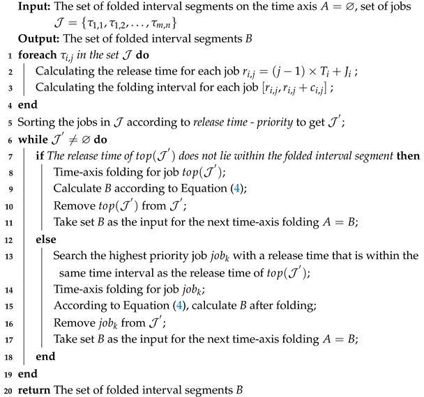
Task-scheduling algorithms in real-time systems can be classified into two categories based on their preemption behavior: preemptive scheduling algorithms and non-preemptive scheduling algorithms. In the case of preemptive scheduling policies, a job may be interrupted during its execution by a higher-priority job. The interrupted job can then resume execution after the higher-priority job is released. In this case, the time axis is temporally folded from high to low according to the priority of the job, and the folding algorithm is shown in Algorithm 1. Lines 1–4 generate folding start points and intervals to be folded based on the job set; line 5 sorts the jobs by their priority and then folds them in descending order of priority. Lines 6–11 complete the folding of all jobs according to Equation (4), line 12 returns all the folded interval segments after after all folding is completed. The PBTF algorithm ensures the correct simulation of preemption operations while avoiding the overhead introduced by preemption operations, effectively reducing the frequency of system state updates during the simulation process.

Algorithm 1: Job Priority-Based Time-axis Folding Algorithm (PBTF)

For non-preemptive scheduling, the job is not allowed to be interrupted during execution, and after the job is released, it will be executed until completion. In this case, the time axis is folded from front to back according to the order of the release time of the jobs, and the folding algorithm is outlined in Algorithm 2. Lines 1–4 generate folding start points and intervals to be folded based on the job set; line 5 sorts the jobs according to release-time priority; line 6 checks whether the folding is complete. Lines 7–12 handle the case where the folding starting point is within a folded interval segment; lines 13–17 handle the case where the folding starting point is outside of the folded interval segment; line 20 returns all the folded interval segments after all folding is completed. The algorithm iterates and folds the jobs until all jobs are folded.   

Algorithm 2: Job Release Time-Based Time-axis Folding Algorithm (RBTF)

   Since jobs are not allowed to be interrupted during execution, there may be more than one job release in the process of job execution. In such cases, the job with the highest priority is chosen for execution next. Thus, in the time-axis folding algorithm, when multiple job release times coincide within a folded interval segment, the job with the highest priority is selected as the one to be folded, as specified in lines 13–17 of Algorithm 2.

The above describes the time-axis folding approach based on priority and release time, respectively, which can be used to calculate the response time of the job in real-time systems and thus complete the schedulability analysis of the task.

Assuming that the set of folded interval segments of the original time axis is $A=\{{\xi }_1,{\xi }_2,\dots ,{\xi }_n\}$, the folding starting point is $r_{i,j}$, the folding length is $c_{i,j}$, and the effective length of $(r_{i,j},o)$ is $c_{i,j}$; then the response time of the job can be calculated according to Equation (5).

$$R_{i,j}=\left\{\begin{array}{cc}{c}_{i,j},\hfill & \forall {\xi }_i\in A,({\xi }_i^S,{\xi }_i^E)\cap (r_{i,j},o)=⌀\hfill \\ c_{i,j}+\underset{n\le m}{max}\sum _{k=1}^n\left|{\xi }_k\right|,\hfill & \exists n\le m,r_{i,j}<{\xi }_n^S\wedge {\xi }_n^E<o\hfill \\ ({\xi }_i^E-r_{i,j})+c_{i,j}+\underset{n\le m}{max}\sum _{k=1}^n\left|{\xi }_k\right|,\hfill & (\exists n\le m,r_{i,j}<{\xi }_n^S\wedge {\xi }_n^E<o)\wedge (\exists {\xi }_i\in A,{\xi }_i^S<r_{i,j}<{\xi }_i^E)\wedge (\forall {\xi }_l\in A,o\notin [{\xi }_l^S,{\xi }_l^E])\hfill \\ c_{i,j}+\underset{n\le m}{max}\sum _{k=1}^n\left|{\xi }_k\right|,\hfill & (\exists n\le m,r_{i,j}<{\xi }_n^S\wedge {\xi }_n^E<o)\wedge (\forall {\xi }_i\in A,r_{i,j}\notin [{\xi }_i^S,{\xi }_i^E]\wedge (\exists {\xi }_l\in A,o={\xi }_l^S)\hfill \\ ({\xi }_i^E-r_{i,j})+c_{i,j}+\underset{n\le m}{max}\sum _{k=1}^n\left|{\xi }_k\right|,\hfill & (\exists n\le m,r_{i,j}<{\xi }_n^S\wedge {\xi }_n^E<o)\wedge (\exists {\xi }_i\in A,{\xi }_i^S<r_{i,j}<{\xi }_i^E)\wedge (\exists {\xi }_l\in A,o={\xi }_l^S)\hfill \end{array}\right.$$

(5)

Equation (5) divides the job response time analysis into five cases, as detailed below:

1.

The set of folded interval segments in the time axis is empty; when the job response time is equal to the job execution time, $R_{i,j}=c_{i,j}$.

2.

Between the folding starting point and the folding endpoint, there may exist multiple folded interval segments, with neither the folding starting point nor the folding endpoint coinciding with any of these folded interval segments. As such, the job response time is the sum of the job execution time and the covered folded interval segments, namely $R_{i,j}=c_{i,j}+\underset{n\le m}{max}{\sum }_{k=1}^n\left|{\xi }_k\right|$.

3.

Only the folding starting point falls within the folded interval segments, and multiple folded interval segments are covered between the starting and endpoints. At this time, the response time $R_{i,j}=({\xi }_i^E-r_{i,j})+c_{i,j}+\underset{n\le m}{max}{\sum }_{k=1}^n\left|{\xi }_k\right|$.

4.

Only the folding endpoint falls within the folded interval segments, and multiple folded interval segments are covered between the starting and endpoints. At this time, the job response time $R_{i,j}=c_{i,j}+\underset{n\le m}{max}{\sum }_{k=1}^n\left|{\xi }_k\right|$.

5.

The folding starting point falls within a folded interval segment and the folding endpoint coincides with a folded interval segment. At this time, the job response time $R_{i,j}=({\xi }_i^E-r_{i,j})+c_{i,j}+\underset{n\le m}{max}{\sum }_{k=1}^n\left|{\xi }_k\right|$.

The time metrics of systems are then obtained by sampling task execution intervals across multiple simulation runs; following a Monte Carlo-like strategy, the worst-case response time $WCR{T}_{{\tau }_i}$ is calculated as Equation (6):

$$WCR{T}_{{\tau }_i}=\underset{k}{max}{R}_{i,j}$$

(6)

The best-case response time $BCR{T}_{{\tau }_i}$ is calculated as Equation (7):

$$BCR{T}_{{\tau }_i}=\underset{k}{min}{R}_{i,j}$$

(7)

The response time jitter is calculated as Equation (8):

$$RT{J}_{{\tau }_i}=WCR{T}_{{\tau }_i}-BCR{T}_{{\tau }_i}$$

(8)

where $RT{J}_{{\tau }_i}$ indicates response time jitter of task ${\tau }_i$.

5. Multi-Core Global Scheduling Response Time Analysis

5.1. Core-Mapping Conflicts

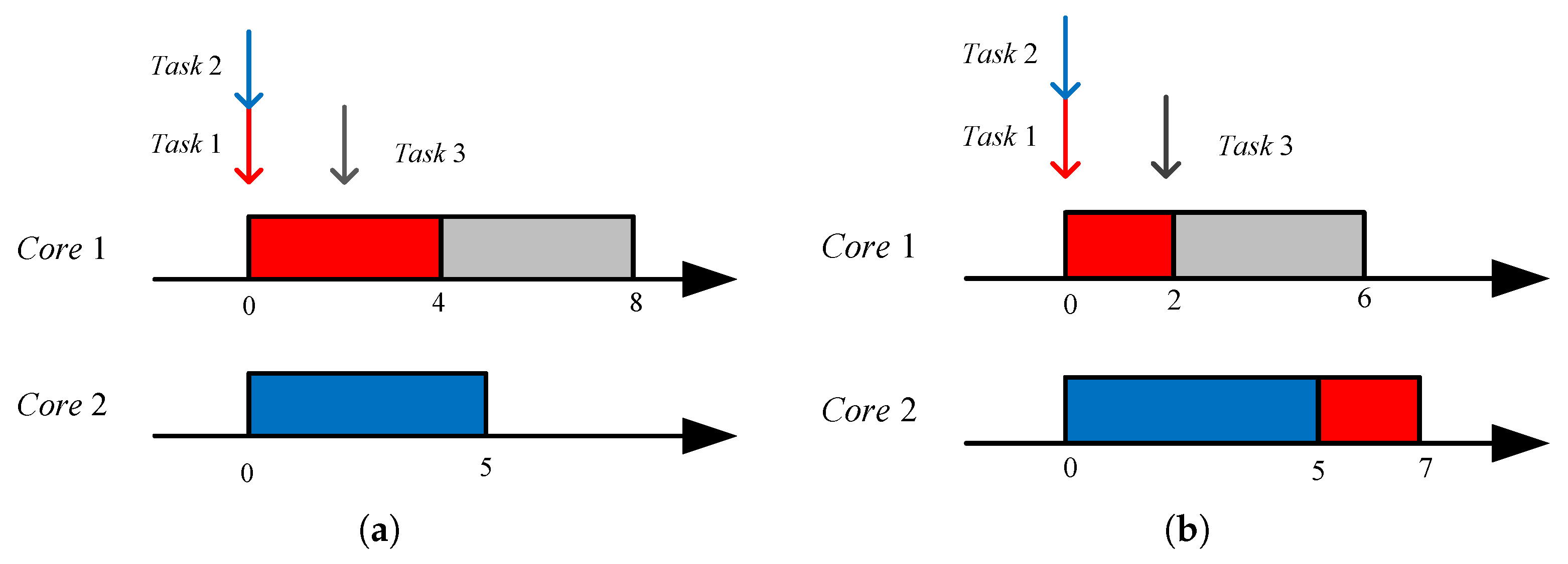
As described in Section 4, the job execution process can be viewed as a time-axis folding process. In the context of preemptive scheduling for a single-core processor, it is possible to arrange jobs in descending order of priority, as exemplified by the PBTF algorithm. In contrast, for non-preemptive scheduling, the arrangement of jobs can be based on their release times, as illustrated by the RBTF algorithm. When considering a multi-core global scheduling algorithm, the utilization of the PBTF algorithm is unfeasible due to the inability to predict the mapping relationship between jobs and processors in advance. A direct application of the RBTF algorithm may lead to core-mapping conflicts, as illustrated in Figure 3.

Task 1, Task 2, and Task 3 have low, medium, and high priorities, respectively. Their release times are 0, 0, and 2, and their execution times are 4, 5, and 4, respectively. In Figure 3, the simulation results obtained using the RBTF algorithm show a core-mapping conflict between Task 1 and Task 3 compared with the actual execution scenario, leading to inconsistent task response times.

To address this issue, a time-axis unfolding algorithm is proposed. Combined with the RBTF algorithm, this mechanism reclaims the suspended latter portions of tasks back to the ready queue, thereby resolving core-mapping conflicts and enabling dynamic job-to-core mapping in global scheduling simulations.

5.2. Time-Axis Unfolding Algorithm

Time-axis unfolding is the inverse operation of time-axis folding, which is to restore the folded time interval on the time axis to an unfolded state. As shown in Figure 4, on the basis of the initial time axis $t_0$, the folded time axis is obtained by folding the time interval (5, 9), and the folded interval segment is A: [5, 9] at this time. Subsequently, the time interval (7, 9) is unfolded to obtain the unfolded time axis, and the folded interval segment is A: [5, 7] at this moment.

The time-axis unfolding algorithm has the following constraints:

1.

The initial time axis $t_0$ cannot be unfolded.

2.

The unfolded time interval $[a,b]$ should be continuous.

3.

The unfolded time interval $[a,b]$ should fall within a certain folded interval segment.

The set of folded interval segments of time axis t is denoted as $A=\{{\xi }_1,{\xi }_2,\dots ,{\xi }_n\}$. After the time interval $[a,b]$ is unfolded, the set B of unfolded folded interval segments can be computed as shown in Equation (9).

$$B=\left\{\begin{array}{cc}A-{\xi }_i,\hfill & \exists {\xi }_i\in A,{\xi }_i^S=a,{\xi }_i^E=b\hfill \\ (A-{\xi }_i)\cup (b,{\xi }_i^E),\hfill & \exists {\xi }_i\in A,{\xi }_i^S=a,{\xi }_i^E>b\hfill \\ (A-{\xi }_i)\cap ({\xi }_i^S,a),\hfill & \exists {\xi }_i\in A,{\xi }_i^S<a,{\xi }_i^E=b\hfill \\ (A-{\xi }_i)\cap ({\xi }_i^S,a)\cap (b,{\xi }_i^E),\hfill & \exists {\xi }_i\in A,{\xi }_i^S<a,{\xi }_i^E>b\hfill \end{array}\right.$$

(9)

When the unfolded time interval perfectly aligns with a specific point on the time axis, that particular folded interval segment is removed from set A of folded interval segments. However, if the time interval to be unfolded only partially overlaps with a folded interval segment, the act of unfolding the folded interval segment results in the creation of a new folded interval segment, which then takes the place of the original folded interval segment.

5.3. Dynamic Core Mapping

The RBTF algorithm cannot capture the task preemption process in multi-core global scheduling, which leads to core-mapping conflicts. To represent the scenario where higher-priority jobs preempt lower-priority ones, priorities are assigned to folded interval segments and the time intervals to be folded. These priorities are used to determine the relative priority between a time interval to be folded and the folded interval segments on the time axis. Subsequently, the folded interval segment is denoted as ${\xi }_i=\langle [{\xi }_i^S,{\xi }_i^E],{\pi }_i\rangle$, where ${\pi }_i$ denotes the priority of the folded interval segment. The time interval to be folded is denoted as ${[a,b]}_{\pi }$, where $\pi$ denotes the priority of the time interval. When the folded interval segments on the time axis intersect with the high-priority time intervals to be folded, the folded interval segments need to be folded. When the time interval to be folded is merged with the original folded interval segment, the determination of its priority follows the principle of priority inheritance, as described below.

Theorem 1.

(Priority inheritance) The priority of a folded interval segment after the merging of two neighboring folded interval segments is inherited from the priority of the higher folded interval segment, that is

$${\pi }_U=\left\{\max ({\pi }_a,{\pi }_b)\right|{\xi }_U={\xi }_a\cup {\xi }_b,{\xi }_a^E={\xi }_b^S\}$$

(10)

In the RBTF algorithm, the folding starting point is the release time of the job. However, in the context of static priority preemptive global scheduling for multi-core processors, where task preemption is a factor, the folding starting point encompasses not just the job’s release time but also the moment at which the job’s execution resumes. This resumption time is dependent on the completion time of a higher-priority task which was previously being executed. Therefore, the folding starting point includes two categories: one is the release time of the job, which is calculated by $r_{i,j}=(j-1)\times T_i+J_i$, and the other is the time of resuming the execution of the job, which needs to be analyzed and derived in the simulation process. The time when the job is preempted needs to be considered only for the starting point of the unfolding interval.

Proof of Theorem 1.

For a multi-core processor $P=\{c_1,c_2,\dots ,c_n\}$, n denotes the number of cores, each core corresponds to a time axis, the set of time axes $A=\{A_1,A_2,\dots ,A_n\}$, and each of time axis $A_k=\{{\xi }_{k\_1},{\xi }_{k\_2},\dots ,{\xi }_{k\_m}\}$, where m denotes the number of folded interval segments. The cases where an idle core exists, where the folding interval does not overlap with existing folded interval segments, or where the priority of the folding time interval is lower than that of all folded interval segments on the time axis will be excluded from discussion, as these situations are straightforward and their handling is self-evident. Instead, focus will be placed on the scenario where the priority of the folding interval is at least equal to that of all folded interval segments on the time axis $\exists A_k,{\xi }_i\cap \widehat{(a,a+\Delta t)}\ne ⌀,{\pi }_x>{\pi }_k$. In this case, whether the priority of the folding interval exceeds that of all folded interval segments or higher-priority folded interval segments, the folding process will only affect the previously folded interval. As a result, the only action required will be to expand the folding time interval of the preceding time interval. This is because the start point of the folding interval cannot occur before the start point of the previously folded interval.    □

Assuming that the release time of job $jo{b}_k$ is a, WCET is $\Delta t$, and the corresponding to-be-folded time interval takes a as the folding starting point and $\Delta t$ as the folding duration. The dynamic core-mapping algorithm can be denoted as shown in Equation (11).

$$\begin{array}{c}\hfill f(A,a,\Delta t)=\left\{\begin{array}{cc}{A}_{\min }\left(k\right)\mapsto \widehat{(a,a+\Delta t)},\hfill & \exists A_k=⌀\hfill \\ A_{\min }\left(k\right)\mapsto (A_{\min }\left(k\right)\cup \widehat{(a,a+\Delta t)}),\hfill & \exists {\xi }_i\in A,a\ge {\xi }_i^E\hfill \\ A,\hfill & \forall A_k,\exists {\xi }_i\cap \widehat{(a,a+\Delta t)}\ne ⌀,{\pi }_x<{\pi }_i\hfill \\ A_{\min }\left(k\right)\mapsto ((A_{\min }\left({\pi }_k\right)-{\xi }_i)\cup \widehat{({\xi }_i^S,a+\Delta t)}),\hfill & \exists A_k,{\xi }_i\cap \widehat{(a,a+\Delta t)}\ne ⌀,{\pi }_x>{\pi }_k\hfill \end{array}\right.\end{array}$$

(11)

1.

In instances where there exists no folded interval segment within the time axis corresponding to a core, the time interval earmarked for folding is allocated to the time axis possessing the lowest numerical identifier. Such a situation arises when a specific processor core has never been assigned a job.

2.

When the starting point of the time interval to be folded is greater than the right boundary of all folded interval segments on a given time axis, the time interval to be folded is assigned to the time axis with the smallest number. This case corresponds to the presence of idle processor cores.

3.

When the time interval to be folded intersects with all folded interval segments on the time axis and the intersection is not null, no folding operation will be executed provided that the priority of this time interval is lower than that of the intersecting folded interval segment.

4.

In the event that the time interval earmarked for folding intersects with every folded interval segment along the time axis, and this intersection is non-empty, if the priority of the said time interval surpasses that of the intersecting folded interval segments, time-axis folding or unfolding is executed on the time axis housing the folded interval segment characterized by the lowest priority. First, time-axis unfolding is performed for this time interval by taking the starting point of the time interval to be folded as the unfolding starting point and the endpoint of the folded interval segment intersecting with it as the unfolding endpoint. Then, time-axis folding is performed by taking a as the folding starting point and $\Delta t$ as the folding duration. The priority of the folded interval segments obtained after folding is determined according to the principle of priority inheritance.

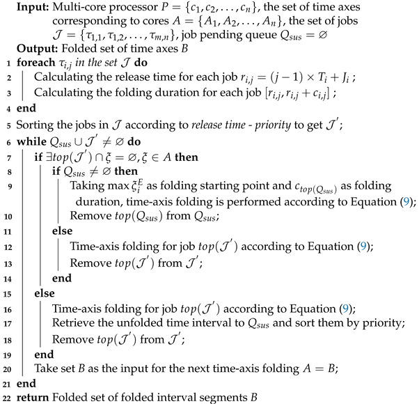
Based on the above analysis, the schedulability analysis method EvoSMS, which is based on increasing release times and core-mapping conflict mitigation, is designed as shown in Algorithm 3. Lines 1–4 generate folding start points and intervals to be folded based on the job set; line 5 sorts the jobs according to release time priority; line 6 checks the job set and the jobs reclaimed due to time-axis unfolding to determine whether the folding is complete. Lines 7–14 handle the case where the earliest-release-time job in the job set intersects with a folded interval segment on the time axis: lines 8–10 indicate that if the suspended job set is not empty, suspended jobs are folded first; lines 11–13 indicate that if the suspended job set is empty, the earliest-release-time job in the job set is folded. Lines 15–18 handle the case where the earliest-release-time job does not intersect with any folded interval segments on the time axis, folding the job directly. Line 20 sets the time-axis collection obtained in the current folding iteration as the input for the next iteration, and the process is repeated until all jobs are folded. Line 22 returns all the folded interval segments after all folding is completed. The time complexity of lines 1–4 is $O\left(n\right)$, where n denotes the size of the job set. Line 5 employs a priority queue implementation with a time complexity of $O\left(logn\right)$, and lines 6–19 have a time complexity of $O\left(n\right)$. Therefore, the overall time complexity of Algorithm 3 is $O\left(n\right)$.

Algorithm 3: An Event-Oriented Simulation Method for Multi-Core Real-Time Scheduling (EvoSMS)

5.4. Simulation Efficiency Analysis

To assess the progress of this approach in terms of simulation efficiency, the number of system state updates serves as an evaluation metric to analyze how the calculation of the number of system state updates differs between the process-oriented simulation approach and the event-oriented simulation approach, respectively.

The process-oriented simulation approach is clock-driven, and its system state update times are positively correlated with the number of clock advances and the number of tasks. Assuming that the problem window is $PB$ and the number of tasks is n in the system, the system state update times $N_P$ for the process-oriented simulations can be calculated as follows:

$$N_P={\sum }_{i=1}^{PB}{Q}_i$$

(12)

where $Q_i$ indicates the number of jobs present in the system at time i. It can thus be inferred that the number of system state updates triggered by job is equal to the time that the job resides in the system, which corresponds exactly to the response time of the job. Assuming that the set of tasks in the system $\mathrm{\Gamma }=\{{\tau }_1,{\tau }_2,\dots ,{\tau }_n\}$ and the period of task ${\tau }_i$ is $T_i$, the number of simulations $N_E$ can be calculated as follows within the problem window $PB$ time. Therefore, the total number of system state updates in a process-oriented simulation algorithm is equal to the sum of the response times of all jobs in the system, expressed as follows:

$$N_P={\sum }_{i=1}^n{\sum }_{j=1}^{⌊{\displaystyle \frac{PB}{T_i}}⌋}{r}_{i,j}$$

(13)

In terms of the event-oriented simulation approach, the number of simulations is not related to the clock but is positively related to the number of events and consequent event in the simulation process. For the EvoSMS algorithm, if the time interval to be folded intersects with a folded interval segment on the time axis, the folded interval segment will be unfolded and must be folded again. Based on this, we provide a method for calculating the number of system state updates in the event-oriented simulation algorithm.

$$N_E={\sum }_{i=1}^n{\sum }_{j=1}^{⌊{\displaystyle \frac{PB}{T_i}}⌋}k$$

(14)

If the time interval to be folded does not intersect with any folded interval segment, then $k=1$; otherwise, $k=2$. Based on the aforementioned analysis, the number of system state updates in a process-oriented simulation algorithm can be smaller than that of an event-oriented simulation algorithm only when the response times of all jobs are less than 2.

6. Experiments and Result Analysis

In order to verify the analysis accuracy and time performance of the EvoSMS algorithm, three sets of comparison experiments were conducted in the present study to verify the superiority of the approach.

6.1. Experiment Platform

All experiments were conducted on a desktop computer with a 3.2 GHz Core (TM) i7-8700 CPU and 8 GB of RAM, running a Windows 10 operating system. We implemented the EvoSMS algorithm based on Java, with JDK version 1.8 and SimSo version 0.8.3 as the comparative experimental tool.

6.2. Comparison of Task Response Time Analysis Precision

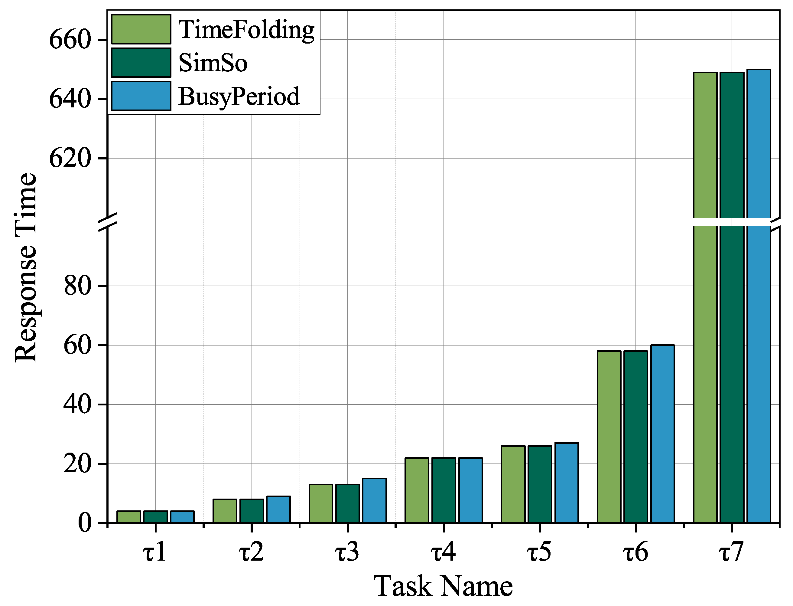
To verify the accuracy of the task response time analysis method based on time folding, we conducted comparative experiments between the proposed approach, the conventional busy-window response time analysis method, and other simulation-based approaches. The task parameters used in the experiments are listed in

Table 3. Task parameter configuration.

Task Name	Priority	Release Jitter	Execution Time	Period
${\tau }_1$	1	1	4	30
${\tau }_2$	2	2	5	30
${\tau }_3$	3	3	6	30
${\tau }_4$	4	1	7	30
${\tau }_5$	5	2	5	50
${\tau }_6$	6	3	6	50
${\tau }_7$	7	2	7	50
${\tau }_8$	8	1	8	50

. A smaller task priority value indicates a higher priority, and the scheduling policy is fixed-priority preemptive scheduling. The problem window is set to [0, 1000].

The experimental results are shown in Figure 5, where the horizontal axis represents the task names and the vertical axis represents the worst-case response time. In the figure, “TimeFolding”: denotes the response time analysis results obtained by the proposed time-folding-based method, “BusyWindow” represents the results derived from the conventional busy-window analysis, and “SimSo” corresponds to the results obtained from the multi-core schedulability simulation tool SimSo.

6.3. Comparison of Global Scheduling Analysis Accuracy for Multi-Core Processors

In this section, the analysis results of the EvoSMS simulation analysis algorithm are compared with those of the SimSo simulator to evaluate the analysis accuracy of the approach through the acceptance rate. The acceptance ratio quantifies the proportion of task examples within the system that meet the schedulability requirement in relation to the total number of task examples. The acceptance ratio can be calculated as shown in Equation (15). It is employed to characterize the schedulability of the entire task set in the system.

$$\eta ={\displaystyle \frac{m_S}{m}}$$

(15)

where $\eta$ is the acceptance ratio of tasks, $m_S$ is the number of schedulable task instances, and m is the total number of task instances. Generally speaking, the higher the acceptance ratio, the better the performance of the schedulability analysis.

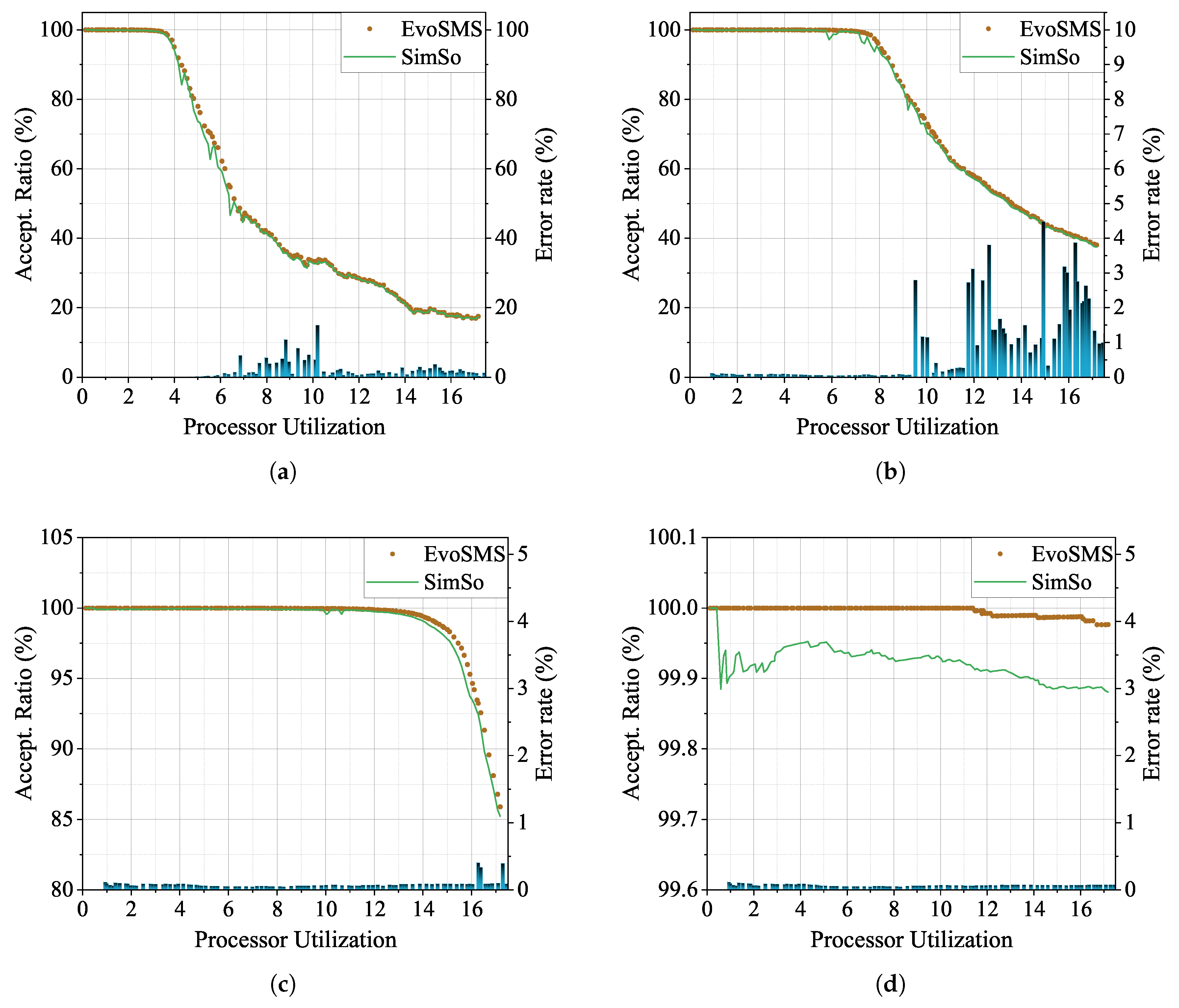
The experimental parameters were set as follows: all task periods obeyed the uniform distribution of [10, 100]; the number of tasks was 150; the task utilization rate obeyed the uniform distribution of [0.05, 0.2]; the release time jitter of tasks obeyed the uniform distribution of [0, 5]; all tasks in the set had implicit deadlines, meaning their deadlines equaled their periods; the problem window was [0, 1000]; the number of cores was set to 4, 8, 16, and 32. The EvoSMS simulation analysis algorithm and SimSo simulator were evaluated under identical parameters as described above. The experimental results are shown in Figure 6.

The horizontal coordinate indicates the total processor utilization, the left axis of the vertical coordinate indicates the acceptance ratio, and the right axis of the vertical coordinate indicates the error rate of the two simulation analysis results, which can be calculated as shown in Equation (16).

$$\delta ={\displaystyle \frac{{\xi }_{EvoSMS}}{{\xi }_{SimSo}}}\times 100\%$$

(16)

The curve EvoSMS in the figure represents the multi-core response time analysis approach based on time-axis folding and unfolding proposed in the present study, and SimSo corresponds to the analysis results derived from the simulation tool SimSo.

The experimental results shown in Figure 6 indicate that the task acceptance rate tended to decrease as the sum of processor utilization continued to grow. When comparing the task acceptance rates between the two analysis approaches, it becomes evident that the proposed EvoSMS approach exhibited a marginal performance advantage over the SimSo simulator. According to statistical calculations, when the number of cores N = 4, the task acceptance rate was improved by 1.49% on average; when N = 8, it was improved by 0.9% on average; when N = 16, it was improved by 0.24% on average; when N = 32, it was improved by 0.08% on average.

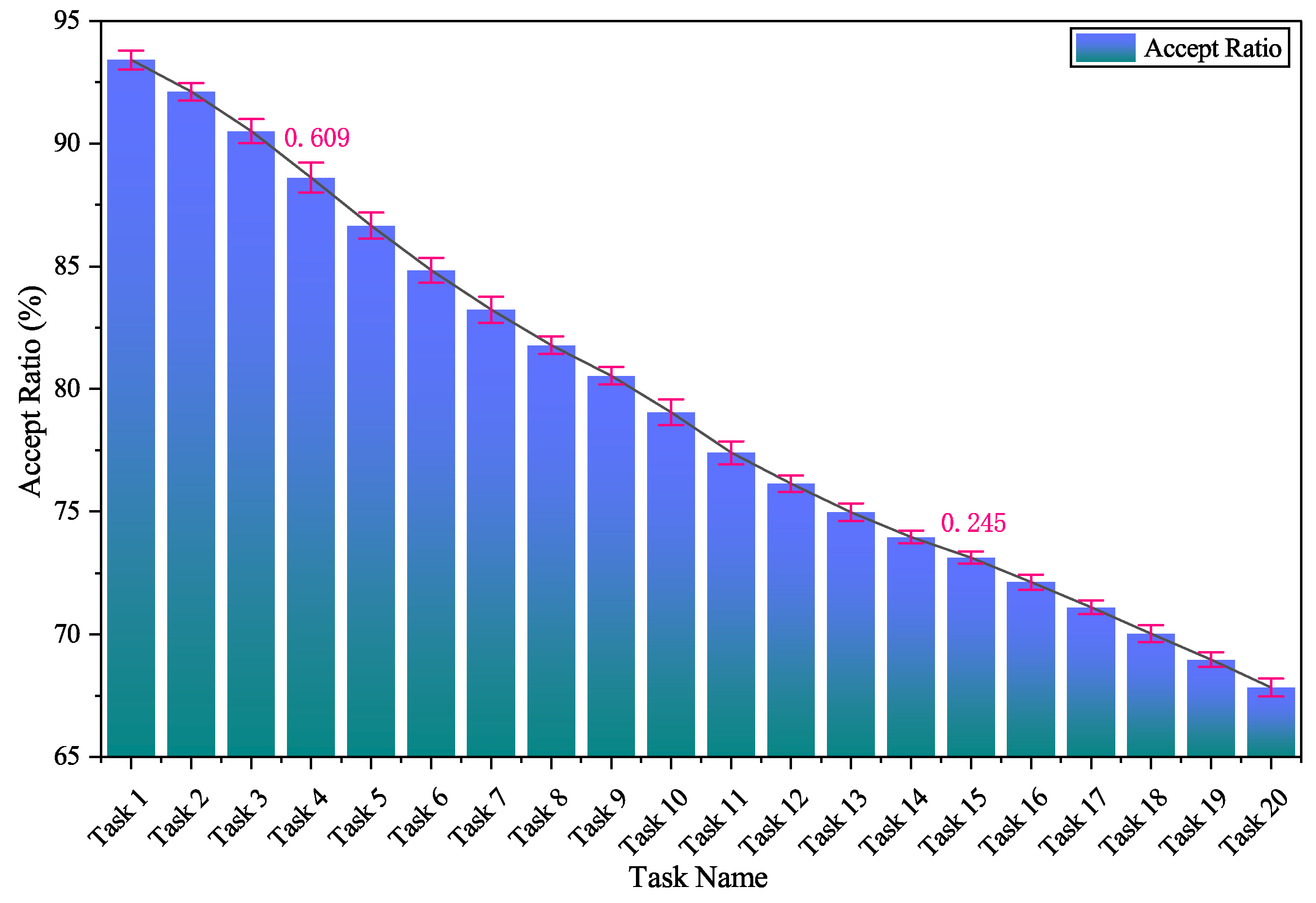
To demonstrate the robustness of the proposed method, the variability of the acceptance ratio was analyzed over 200 simulations for 20 task sets, as shown in Figure 7; the x-axis represents the task names, the y-axis represents the task acceptance rates, and the pink error bars represent the standard deviation. As presented in Figure 7, the maximum standard deviation is 0.609%, while the minimum standard deviation is 0.245%, indicating that the proposed method exhibits good robustness.

6.4. Simulation Time Comparison

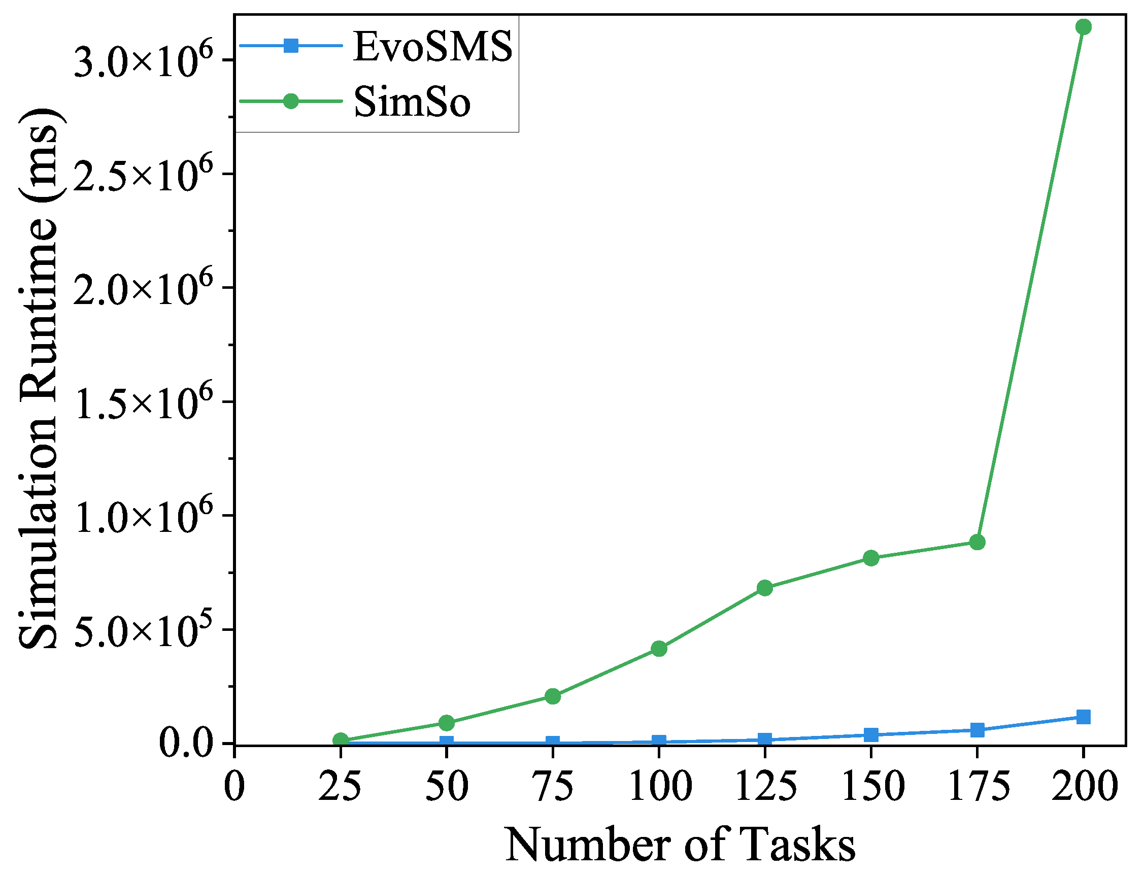
In this section, the simulation duration of the EvoSMS simulation analysis algorithm is compared with that of the SimSo simulator to evaluate the advantages of the proposed approach in terms of simulation efficiency. This comparison was carried out under identical parameters as follows: all task periods obeyed the uniform distribution of [10, 100]; the task utilization rate obeyed the uniform distribution of [0.05, 0.2]; the release time jitter of tasks obeyed the uniform distribution of [0, 5]; all tasks within the set had implicit deadlines, meaning their deadlines equaled their periods; the problem window was [0, 3000]; the number N of processor cores was 8; and the number of tasks was set to 25, 50, 75, 100, 125, 150, 175, and 200, respectively. The experimental results are shown in Figure 8. The horizontal coordinate indicates the number of tasks, and the vertical coordinate, which uses a linear scale, represents the running time of the simulation program. The green line connecting circular markers represents the simulation runtime of SimSo, while the blue line connecting square markers represents the simulation runtime of EvoSMS.

As shown in Figure 8, although the running time of both simulation approaches tended to grow as the number of tasks in the system kept increasing, the running time of the SimSo simulator grew faster and that of EvoSMS was relatively stable. The comparison between the EvoSMS approach and SimSo reveals a substantial advantage in terms of runtime for EvoSMS. Based on the statistical analysis of the experimental results, it was observed that, on average, the simulation runtime of EvoSMS was 96.24% lower than that of SimSo.

7. Conclusions and Future Work

Aiming to address the inefficiency of simulation-based schedulability analysis, this paper introduces an event-oriented simulation strategy and presents the implementation of EvoSMS, which is based on time-axis folding and unfolding algorithms. Experimental results demonstrate the accuracy of the analysis outcomes and highlight the improvements in analysis efficiency offered by the EvoSMS method.

The current work focuses on the actor model with periodic tasks and implied deadlines, which simplifies the analysis but limits the general applicability of the results. Specifically, EvoSMS currently does not handle sporadic tasks or tasks with arbitrary deadlines, restricting its use in more diverse real-time scenarios. In addition, the method is limited to multi-core processors and has not yet been applied to multi-core distributed systems. As part of the planned extensions, the actor model will be enhanced to include message-passing models, and the script model will incorporate bus arbitration mechanisms to enable bus modeling, thereby facilitating further extension to distributed systems.

Another limitation lies in the scope of the modeling: the current approach does not fully account for interruption policies, global/partition scheduling support, or detailed resource models such as buses, caches, and critical sections. These omissions may affect the accuracy and generalization of the evaluation, as real-world systems often involve complex interactions among these factors. Furthermore, the simulation results are dependent on chosen parameters, including task models and execution time assumptions, which may influence observed schedulability outcomes. To address this, EvoSMS provides a set of generic XML files to describe various system models, and key parameters can be refined, for example, by collecting extensive measurements to obtain task execution time distributions.

Future work will address these limitations by extending EvoSMS to handle sporadic tasks and arbitrary deadlines, supporting distributed multi-core systems and incorporating more comprehensive modeling of interruption policies, global and partitioned scheduling, and shared resources (including buses, caches, and critical sections). Additionally, we aim to study the sensitivity of the simulation results to different parameter settings to ensure more robust and generalizable conclusions.